Article

Concept Tree Learner (CTL): An Incremental and Interpretable Symbolic Framework for Binary String Rule Induction

by
Muhammed Tekin Ertekin
* and
Burkay Genç
Department of Computer Engineering, Hacettepe University, Beytepe Campus, 06800 Ankara, Türkiye
*
Author to whom correspondence should be addressed.
Appl. Sci. 2026, 16(17), 8542; https://doi.org/10.3390/app16178542
Submission received: 24 May 2026 / Revised: 23 August 2026 / Accepted: 24 August 2026 / Published: 27 August 2026
(This article belongs to the Section Computing and Artificial Intelligence)

Abstract

Symbolic and rule-based learning offers a transparent, sample-efficient alternative to the statistical paradigm that dominates contemporary machine learning. Whereas large language models and deep networks approximate target functions from massive corpora without exposing the rules they rely on, many practical problems instead call for compact, human-readable concept definitions learned from only a handful of examples. In this paper, we introduce the Concept Tree Learner (CTL), an incremental and interpretable symbolic framework that induces logical concepts over binary strings from minimal labeled data. CTL represents knowledge as a rooted tree of logical predicates; it extends this tree incrementally as each labeled example is processed and, after observing the data, distills the simplest rule set consistent with all examples through a set-cover filtering step, in accordance with Occam’s Razor. We give formal definitions for the tree structure, its construction and pruning operations, and the rule-selection objective, and we analyze the worst-case time and space complexity of the procedure. A prototype implementation, operating over a small set of atomic binary-string predicates whose numeric arguments scale dynamically with the input length, is evaluated across 29 concept-learning tasks of varying complexity. CTL recovers a consistent concept for every task—the intended one on 26 of the 29 datasets, and an equally consistent alternative on the three whose training set does not uniquely determine it—typically converging before all training examples are exhausted, and produces fully interpretable rule sets. On the same atomic vocabulary, it generalizes substantially better to unseen strings than both a classical entropy-based decision tree and the RIPPER (Repeated Incremental Pruning to Produce Error Reduction) rule learner ( 95.5 % mean accuracy across all tasks—and 100 % on the 26 tasks whose training set uniquely determines the target—versus 72.1 % and 77.2 % respectively), while using fewer and shorter rules. We position CTL within the literature on symbolic machine learning, inductive logic programming, and decision-tree induction, discuss the current limitations of the prototype—its restriction to noise-free binary input, its batch (sorted) training regime, and its fixed predicate vocabulary—and outline concrete directions for extending it toward a self-expanding, hierarchical concept-learning system.

1. Introduction

Artificial Intelligence (AI) is a field of computer science and a set of emerging technologies that are used to make computers learn, reason, and perform just like a human being, relatively faster and more efficiently. In recent years, the scope and application domains of AI have expanded significantly. The umbrella term now contains various subdisciplines, including machine learning, deep learning, natural language processing, and computer vision. It can be said that AI covers the capacity of computational systems to execute tasks generally requiring human cognitive abilities, including learning, reasoning, problem-solving, perception, and decision-making processes [1].
Classical machine learning approaches use a well-structured dataset to learn patterns and then use the learned knowledge to make classification or regression predictions on new and unexplored data. Similarly, deep learning models use more complicated data inputs and can even generate output similar to the input. Finally, large language models learn and mimic human languages using billions of textual documents. However, none of these approaches actually learn the concepts within the data to be able to derive new concepts. An AI model that can learn from existing knowledge and then synthesize this knowledge to create and learn new concepts without even being trained on them is called Artificial General Intelligence (AGI). To this day, a working and fully autonomous AGI has not been developed.
LLMs like GPT-4, DeepSeek, and Gemini demonstrate significant capabilities for many tasks, but they still fall short of true AGI. For example, they can generate text and answer questions based on patterns in their training data, but they cannot truly understand context or reason like a human. They cannot identify the real semantic patterns behind the data because of their probabilistic nature.
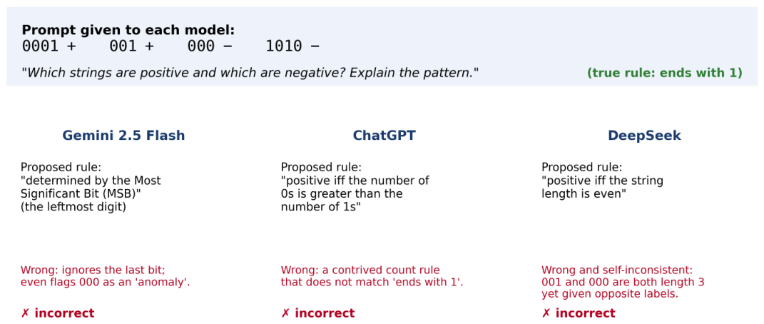
In Figure 1, the responses of three popular LLMs are shown when asked to recognize the pattern in a short input of four binary strings. Although multiple patterns can be detected in this input, we are always looking for the shortest and most concise pattern as we will later discuss in detail. In this input, as any human can quickly recognize, strings ending with “1” are positive and strings ending with “0” are negative. In such a simple example, we observe that all three LLMs fail to recognize the pattern. These models are trained to statistically produce text, and they struggle to understand these kinds of semantic patterns. Interestingly, this small puzzle is almost trivial for any human being.
AGI, also referred to as human-level artificial intelligence, represents a category of artificial intelligence systems that can demonstrate cognitive capabilities equivalent to or exceeding those of humans across virtually all intellectual domains [2,3]. There exists ongoing debate among researchers regarding the current state of AGI development. Although there are claims that contemporary large language models (LLMs) already demonstrate characteristics indicative of AGI-level performance, others assert that authentic AGI remains an unrealized goal [4]. When we consider the example above, we tend to side with the latter.
In this study, we adopt a complementary, bottom-up perspective on concept acquisition. A long line of work in cognitive science and developmental psychology characterizes human learning as compositional and incremental: complex concepts are constructed by combining simpler, previously acquired ones, rather than being inferred wholesale from large volumes of data [3,5]. In language acquisition, for instance, phonemes are combined into syllables, syllables into words, and words into sentences, yielding a hierarchy in which higher-level units are defined in terms of lower-level ones [5]. This compositional view motivates a learning architecture that begins from atomic concepts and composes them into progressively more complicated ones, and it is the inductive bias we operationalize in this paper. We emphasize that invoking this analogy is a design motivation only; we make no claim that the proposed system reproduces human cognition.
This clearly distinguishes our approach from existing statistical learning tools, no matter how complicated and powerful they are. For example, LLMs do not try to understand the structure of a language like a baby. They learn top-down: we feed them huge amounts of text and from this text they learn how to produce the next letter in a streaming partial text. They do not really consider what they will say in a second, or what they were talking about a minute ago. All they consider is the statistical sequencing of the letters in a chunk of text.
In this paper, we focus on the most elementary building block of such a compositional system: learning interpretable logical concepts over binary strings from minimal labeled data. We choose binary strings as the substrate for two reasons. The first is pragmatic: it is the simplest non-trivial domain in which compositional, trimming-based predicate induction can be defined and studied in a controlled way. The second is that binary strings are a universal encoding—any digital artifact, from a numeric identifier to an image, is ultimately a sequence of bits. We are careful not to overstate this second point: universality of the encoding does not by itself imply that the bit level is the right level of abstraction for learning every concept (a concept such as “is a photograph of a cat” is hopeless to learn directly over raw pixels with predicates like ours). What it does provide is a uniform, minimal starting representation in which a concept, once learned, can in principle serve as a primitive in a higher-level concept. The present work does not attempt to build such hierarchies; it establishes and rigorously evaluates the base learner over the simplest bit-level concepts, which is a prerequisite for any later hierarchical composition.
We make the scope of our contribution explicit. We do not claim a system that exhibits autonomous reasoning, invents its own predicates, or generalizes across arbitrary domains; the prototype searches a finite, human-specified hypothesis space built from a small set of atomic predicates. What we contribute is (i) a formally defined, incremental algorithm that induces a compact, fully interpretable rule set for a target concept from very few examples; (ii) a dynamic predicate-argument scheme and a set-cover-based filtering step that keep the learned rule set minimal in the spirit of Occam’s Razor; (iii) a worst-case complexity analysis of the procedure; and (iv) an empirical comparison, on a shared atomic vocabulary, against a classical decision-tree learner that quantifies the advantage of the Concept Tree Learner (CTL) in generalization and rule compactness. Extending this base learner toward self-expanding, hierarchical concept formation—a long-term goal aligned with the broader pursuit of more general artificial intelligence—is left to future work.
Our main data structure is a tree that stores the bit strings given as input for each concept. In other words, each learning process focuses on a single concept and produces a unique tree. Unlike classical machine learning, we assume no noise or anomalies in the input data. Also, we assume extremely short and concise learning input to comprehend a concept, unlike statistical learning, where one needs as much data as possible to train a more accurate model. Indeed, we already achieve an understanding of the concept after the processing of the first input, and with each additional input we improve our understanding of the concept.
In the next section, we will look at the literature and examine similar or preliminary studies. Then, we will outline our methodology. Finally, we will provide results and conclusions.

2. Related Works

When examining the literature on AGI, we observe various studies. Some of these studies focus on the ethical and legal dimensions of AGI, as discussed by Bikkasani et al. [6], Sonko [7], Baum [8], and Buttazzo [9]. Others debate whether LLMs have reached AGI-level capabilities, with significant contributions from Emmert-Streib et al. [10], Mumuni and Mumuni [11], Ge et al. [12], and Javaid et al. [13]. Some researchers, including Joshi et al. [14], Korinek and Stiglitz [15], Krause et al. [16], and Bara et al. [17], investigate what developments might occur in various sectors when AGI is achieved. Some studies also aim to achieve AGI by combining different models, as explored by Yao et al. [18], Potapov et al. [19], and Yue et al. [20].

Symbolic Learning, Decision Trees, and Inductive Logic Programming

Because CTL induces explicit logical rules and organizes them in a tree, it belongs to the long-established tradition of symbolic machine learning rather than to statistical learning, and it should be positioned with respect to that literature. The most influential family is that of decision-tree induction. Quinlan’s ID3 [21] builds a classification tree top-down by recursively selecting, at each node, the attribute that maximizes information gain (equivalently, minimizes entropy), and was later extended into C4.5 [22], which adds support for continuous and missing attribute values and performs post hoc pruning to control over-fitting. The CART (Classification and Regression Trees) algorithm [23] is a closely related formulation based on the Gini impurity. These methods are powerful and widely used, but they share three properties that distinguish them sharply from our approach: (i) they operate in batch mode on a fixed feature matrix and must, in general, rebuild the tree when new data arrive; (ii) each internal node performs a single axis-aligned split on a pre-engineered feature, so the rules they express are limited to conjunctions of such features and cannot directly capture structural predicates over a raw string (e.g., “ends with the substring 00”) without explicit feature engineering; and (iii) the splitting criterion is statistical, so reliable trees typically require many examples.
A second, more closely related family is inductive logic programming (ILP), which learns first-order logical rules from positive and negative examples [24,25]. FOIL [26] is the canonical example: it greedily constructs Horn clauses, adding literals one at a time using a gain heuristic analogous to information gain, and is in spirit the closest classical method to CTL because it, too, derives explicit logical rules from labeled examples. CTL differs from FOIL and related ILP systems in three respects. First, FOIL produces a flat list of clauses obtained by greedy, locally optimal literal selection and can become trapped in local optima, whereas CTL maintains many candidate hypotheses simultaneously as distinct paths of a single hierarchical tree and only commits to a final rule set after all data have been seen, through a global set-cover step. Second, CTL is incremental: each new example only locally extends the existing tree rather than triggering a re-search of the clause space. Third, CTL’s trimming (cutting) variants let atomic predicates be composed along a path to express longer structural patterns (for example, chaining two “ends-with-0” predicates to recognize multiples of four), which gives the path representation an explicit compositional, inheritance-like structure. Like classical rule learners, and unlike opaque neural models, CTL’s outputs are fully inspectable, aligning it with the goals of interpretable and explainable AI [27]. We share with these classical methods the reliance on a human-provided predicate vocabulary; automatic predicate invention remains, for CTL as for much of ILP, an open problem that we discuss as future work.
Recent advances in transformer architectures for Reinforcement Learning (RL) have demonstrated significant improvements in decision-making capabilities. Chen et al. [28] introduced the Decision Transformer, which reframes reinforcement learning as a sequence modeling problem, where transformers are trained to predict actions conditioned on return-to-go, past states, and actions. While this approach shows promising results in offline RL settings, it lacks the explicit symbolic reasoning capabilities that our proposed framework provides, particularly in handling logical constraints and interpretable decision rules.
Zitkovich et al. [29] presented RT-2, a vision-language-action model that directly outputs robot actions from visual and textual inputs, demonstrating the potential of large-scale transformer models in robotics applications. The system learns to ground language instructions in robot actions through co-fine-tuning on robotics and vision-language datasets. However, RT-2’s approach relies primarily on neural pattern recognition without incorporating explicit symbolic reasoning, which limits its ability to handle complex logical operations and systematic generalization that our architecture addresses through its dual reasoning pathways.
Jiang et al. [30] explored learning methods for extracting interpretable logical rules from neural networks while maintaining high performance. Their research demonstrates techniques for incorporating logical constraints into neural learning processes, showing improvements in both accuracy and interpretability. While this approach shares our goal of combining neural and explicit reasoning, our framework extends beyond constraint learning to provide a unified architecture that seamlessly integrates formal manipulation with neural pattern recognition for enhanced problem-solving capabilities.
Shi et al. [31] presented recent developments in multimodal learning, showing significant progress in aligning different modalities through contrastive learning and shared representation spaces. These approaches demonstrate improved performance in tasks requiring cross-modal understanding and generation. However, existing multimodal frameworks primarily focus on statistical correlations between modalities rather than explicit relationships, which our approach addresses by providing structured reasoning mechanisms that can better capture causal and logical relationships across different input types.
Hans et al. [32] emphasized the importance of explicit knowledge representation and logical reasoning in traditional rule-based artificial intelligence approaches. These methods excel in tasks requiring systematic reasoning, explanation generation, and handling of abstract concepts through formal logic systems. While rule-based AI provides strong theoretical foundations for reasoning, it struggles with perception and learning from raw data, limitations that our integrated framework addresses by combining structured reasoning strengths with neural network capabilities for robust real-world applications.
Dhadi et al. [33] investigated research on cognitive architectures like SOAR, examining human-like reasoning processes and decision-making mechanisms in artificial systems. These architectures attempt to model cognitive processes through structured knowledge representation and rule-based reasoning systems. While cognitive architectures provide valuable insights into human reasoning, they often lack the scalability and adaptability that modern neural approaches offer, which our framework bridges by incorporating both structured reasoning and adaptive learning capabilities.
Ibarz et al. [34] demonstrated the power of large-scale pre-training in creating versatile AI systems capable of handling diverse tasks through in-context learning and fine-tuning in their work on foundation models. These models show remarkable emergent capabilities across various domains through scale and data diversity. However, foundation models often operate as black boxes with limited interpretability and struggle with systematic reasoning tasks, challenges that our approach addresses by maintaining transparency and logical consistency while preserving the flexibility and learning capabilities of neural systems.
Reed et al. [35] explored current approaches to neural network integration, examining various methods for combining neural networks with formal reasoning systems, including neural module networks, differentiable programming, and hybrid architectures. These methods show promise in tasks requiring both perception and reasoning capabilities. While existing integration approaches often treat neural and rule-based components as separate modules, our framework proposes a more tightly coupled architecture where logical and neural reasoning complement each other throughout the entire problem-solving process, leading to more coherent and effective decision-making.

3. Methodology

3.1. Research Approach and Rationale

As described in the previous sections, our aim in this study is to develop a concept learning machine that can recognize simple intermediate-level concepts on short binary strings. Our ultimate goal is to extend this work to develop a learning engine that can recognize almost any concept presented as a binary string of arbitrary length. We propose such an engine is the perfect model for mimicking human recognition and learning processes. We now explain how our approach works.
We assume a setup where every concept is expressed via binary strings. These concepts can be as simple as “has at least one 1” or as complicated as “an image of a flower”, their common point being represented as a sequence of bits. Within the boundaries of this study, we focus on only simple mathematical concepts but propose that the idea can be extended to much harder concepts. Each concept is taught to the engine via lines of training input, where each input consists of a bit string and a plus or minus sign. The plus sign denotes that the accompanied bit string matches the concept, and a minus sign denotes the opposite. From this perspective, our engine is a binary classifier of concept existence in provided binary strings.
We will store the knowledge gathered from the input strings in a rooted tree. The branches and leaves of the tree will correspond to different states of input strings and whether those states are positive with respect to the concept or not. Each input string will potentially cause additions and modifications on the tree. Upon processing each input string, the current tree defines the most up-to-date concept model learned. However, the tree may contain and represent more than one intermediate level concepts that match the input string. We assume the shortest explanation (simplest concept) is the preferred one under such circumstances, as it fits the Occam’s Razor principle.
Using a concept tree, one can query new binary strings to see whether they belong to the concept or not. This way a binary classifier is obtained.

3.2. Dataset

We now explain our training datasets for the experiments we have conducted. Each line in the datasets represents a specific input case, where the first part of the line contains a binary string of potentially arbitrary length, and the second part indicates whether this string matches the concept (accepted) or does not match the concept (rejected). Naively, acceptance is represented by “+” whereas rejection is represented by “−”. An example dataset is shown in Table 1. In this dataset, we have 11 lines of input. The concept in this dataset is “evenness”; in other words, the binary string ends with 0. Note that, normally we can learn this concept with a much shorter dataset, but here the dataset is kept long for demonstration purposes.
We stress at the outset that CTL, in its present form, is a batch learner rather than an online or streaming one: the complete labeled dataset is available before learning begins. As an explicit preprocessing step, we order the dataset so that all positive examples precede all negative ones. This ordering is not a hidden trick but a deliberate design choice whose role and consequences we make precise in Section 3.3.2 and Section 4.2: it lets the destruct operation prune invalidated paths safely and without ever discarding a rule that a later positive example would have required, which in turn reduces time and space complexity. The implications of this assumption, and how it could be relaxed to support online or interleaved data, are analyzed as a limitation in Section 4.3.

3.3. Concept Trees

The concept tree is our main data structure where we store the knowledge learned from the input so far. It is built incrementally by each new line of the input. In a sense it is similar to a finite automaton, as it takes as input a string and processes the string through its nodes. However, there are some major differences: the tree is dynamically built as the input is processed, and the accept and reject nodes are not fixed until the last input line is read.
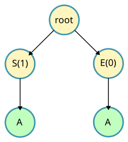
Since the concept tree is a rooted tree, we always start with a root node. The first line of input is then processed. The tree allows a fixed number of node types to be inserted into it. These node types actually correspond to atomic concepts which cannot be divided into simpler concepts. This set of atomic concept nodes is predetermined by us, and it is not necessarily a complete or sufficient set. Indeed finding a complete and sufficient atomic concept set is an interesting problem; however, we do not try to solve this problem in this study. Once we process a line of input, it turns into multiple nodes in the tree, and potentially multiple paths. The leaf nodes can be positive or negative in polarity. Each path that starts from the root node and ends at a leaf node represents an intermediate level concept and the polarity of the leaf node determines whether that concept can explain the inputs or not. In that sense, the tree contains both concepts that can be used to identify the input concept, as well as concepts that cannot be used. Although a single path as defined above can represent an intermediate concept, multiple paths can be taken as a subtree to represent a more complicated intermediate level concept. For example in Figure 2, a simple concept tree that stores two concepts can be seen. The path from the root to the left child goes through two nodes: an s node and an a node. Although, the details of node types will be later provided, we will shortly tell here that s stands for “Starts with” and a stands for “Any”. Together, the path represents a concept of all binary strings that start with a 1, and continue with any string. Similarly, the path that follows the right child from the root represents a concept of all binary strings that “Ends with” a 0. Having these two concepts stored in the tree means the strings in the input all do start with 1 or end with 0.

3.3.1. Formal Definitions

We now formalize the objects introduced above. Let Σ = { 0 , 1 } be the binary alphabet and let Σ * be the set of finite binary strings. To model trimming, we extend the alphabet to Σ X = { 0 , 1 , X } , where X is a placeholder marking a position that has already been consumed and can no longer be matched. A predicate (atomic concept) is a triple p = ( t , a , ρ ) , where t is one of the node types of Table 2, a is its (possibly empty) character/numeric argument, and  ρ { 0 , 1 } indicates whether p is a trimming variant. Each predicate is equipped with two total functions,
acc p : Σ X * { true , false } , τ p : Σ X * Σ X * ,
where acc p decides whether the predicate matches the current string and τ p is the string transformation propagated to the children. For a non-trimming predicate ( ρ = 0 ), we have τ p ( w ) = w ; for a trimming predicate ( ρ = 1 ), τ p replaces the matched characters by X (or removes the leading/trailing one), which guarantees that τ p strictly reduces the number of unconsumed characters and hence that every path terminates. Let P denote the finite set of all predicates obtainable from the eight node types together with their admissible arguments.
A concept tree is a rooted tree T = ( V , E , r ) with root r, in which every non-root node v V carries a predicate p ( v ) P and a status σ ( v ) {active, deleted}. For a node v with ancestor chain r = v 0 , v 1 , , v k = v , the string reaching v when the input w is processed is obtained by the left-to-right composition of the transforms,
w v = τ p ( v k 1 ) τ p ( v 1 ) ( w ) ,
and v accepts w if every predicate on the chain accepts its corresponding intermediate string, i.e., acc p ( v i ) w v i = true for all 1 i k . A root-to-leaf path π thus denotes a rule R π , namely the conjunction of its predicates under progressive trimming, and the set of strings it accepts is its coverage
cov ( π ) = { w Σ * : the leaf of π accepts w } .
The concept represented by a set of active leaf paths Π is their disjunction, and the induced binary classifier y ^ Π : Σ * { 0 , 1 } labels a string positive iff it is covered by at least one selected path:
y ^ Π ( w ) = 1 w π Π cov ( π ) .
The training data is a multiset D = { ( w 1 , y 1 ) , , ( w n , y n ) } with w i Σ * and labels y i { + , } ; write D + and D for the positive and negative subsets. A path π is consistent with D if D + cov ( π ) and cov ( π ) D = . After all data have been processed, the learning objective (formalized in Section 3.3.4) is to return a minimum-cost set of active paths Π whose coverage includes every positive example and excludes every negative one, preferring fewer and shorter paths in accordance with Occam’s Razor. With this vocabulary the operations of the next section read as follows: construct grows V and E so that T contains every path consistent with the positive examples observed so far, destruct sets σ ( v ) = deleted for paths invalidated by a negative example, and the filtering step selects  Π .

3.3.2. Construction

Initially a concept tree is empty except its root node. As we process input data line by line, we mainly do one of two things: either we follow an existing child node or we create new children that match the current string. We then recursively follow each child that matches the current string, as long as there is a matching child and we have not yet hit the tree depth limit.
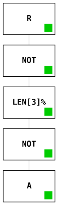
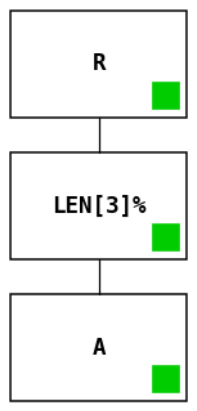
Some node types have two variants: one which does not modify the input string and one that trims the input string. For example, assume a string of “010” reaches an e(0) node with trim variant. The node checks whether the string ends with a 0, and in this case it does. The node then replaces the ending 0 with an X, turning the string into “01X” and passes the modified string to its children. An ‘X’ is a placeholder character representing an already processed bit which cannot be processed any further. Therefore, in practice the string is now reduced to “01”. This ensures that the same node types cannot be applied on a string infinitely and execution must halt eventually. In our node visualizations, we will depict the trim variants with a “%” character. For example, in Figure 3, the ‘LEN[3]%’ node represents the trim variant of the len node with a parameter of 3. For readability, all concept-tree figures in this paper draw only the active nodes of the filtered response; the small green square in the lower-right corner of each node is a status indicator marking it active (the implementation additionally tracks passive and deleted nodes, which are omitted from the figures).
Once a leaf node is reached and the whole input string is processed, the string turns into a concept in the tree: that is a path from the root node to the leaf node. The same string may end up at different leaf nodes of the tree simultaneously. That is due to the fact that there may be more than one concept that describes the same string. If the input string polarity is positive this means the rule represented by this path can be used to describe the concept that the tree is learning. We call such paths “accepted”. However, if the polarity is negative, then this path conflicts with the concept and should be avoided in describing the concept. We call such paths “rejected”. However, a path that is already marked as rejected may later have new children that produce accepted paths. That is one of the most difficult challenges we have faced in constructing our algorithm, and we solve this problem by sorting the input with respect to polarity in the beginning. This way, we process the positive strings first and negative strings later. This, in turn, prevents us from first labeling a path as rejected and then produce longer paths from it labeled as accepted.
The overall build procedure is given in Algorithm 1. When building the tree, we use two fundamental operations: construct and destruct. construct and destruct operations are given in Algorithms 2 and 3, respectively. We now briefly explain each procedure.
The build procedure starts with sorting the input strings with respect to their polarity. This step is very crucial as explained above and avoids early deletion of paths that can be used later. Next, we create the root node of the tree and start processing the input line by line. If we receive a positive input, then we only call the construct procedure. However, for a negative input, we first call the construct procedure and then the destruct procedure. Let us now explain these procedures and the reason behind the different behavior based on the polarity of the input.
Algorithm 1 CTL Build Operation
  1:
procedure Build( d a t a )
  2:
    d a t a . s o r t ( )
  3:
    t r e e CreateRootNode()
  4:
   for all  l i n e in d a t a  do
  5:
        s t r i n g l i n e . s p l i t ( ) [ 0 ]
  6:
        c l a s s _ n a m e l i n e . s p l i t ( ) [ 1 ]
  7:
       if  c l a s s _ n a m e = +  then
  8:
          Construct( t r e e , s t r i n g )
  9:
       else
10:
          Construct( t r e e , s t r i n g )
11:
          Destruct( t r e e , s t r i n g )
12:
        end if
13:
   end for
14:
end procedure
The construct operation simply extends the tree to accommodate the knowledge in a new input line. Its purpose is to check all possible node type, character argument, numeric argument and trim variations to find combinations that can accept the current input string. Then, these combinations are appended to the current node as new children as long as they do not already exist. Next, the processed input string is recursively sent to the newly created children to be further processed until either the tree becomes full or the string becomes empty. The outline of the construct operation is presented in Algorithm 2.
Algorithm 2 Construct Operation
  1:
procedure Construct( t r e e , w o r d )
  2:
   for all t in n o d e _ t y p e s  do
  3:
       for all c in d i c t i o n a r y  do  character variants
  4:
          for  i c min to | w o r d |  do ▹ numeric variants, bounded dynamically by input length
  5:
                for r in { T R U E , F A L S E }  do trim variants
  6:
                   if  n o d e ( t , c , i , r ) . a c c e p t _ s t r i n g ( w o r d )  then
  7:
                         if  t r e e . h a s _ c h i l d ( t , c , i , r )  then
  8:
                             c h i l d t r e e . g e t _ c h i l d ( t , c , i , r )
  9:
                         else
10:
                             t r e e . c h i l d r e n . a p p e n d ( n o d e ( t , c , i , r ) )
11:
                             c h i l d t r e e . g e t _ c h i l d ( t , c , i , r )
12:
                         end if
13:
                         Construct( c h i l d , c h i l d . a f t e r _ p r o c e s s _ s t r i n g ( w o r d ) )
14:
                   end if
15:
                end for
16:
          end for
17:
       end for
18:
   end for
19:
end procedure
An important detail concerns the range of the numeric argument i for the length- and count-based predicates (len and has). Rather than iterating over a fixed, hard-coded interval, the loop on line 4 of Algorithm 2 runs from a small constant c min (we use c min = 2 , the smallest threshold that yields a non-trivial length or count predicate) up to the length | w o r d | of the string currently reaching the node. This bound is principled: a length or count threshold larger than the available string can never be matched, so the dynamic range neither omits any feasible predicate nor wastes work on infeasible ones. Because  | w o r d | shrinks as trimming predicates consume characters along a path, the search space contracts with depth. Consequently the construction adapts automatically to inputs of any length—in particular, strings of length six or more are handled with no change to the algorithm—while simultaneously avoiding the combinatorial blow-up that a fixed, length-independent upper bound would incur on short residual strings. The empirical effect of this choice on tree size is reported in Section 4.2.
For completeness, we state the concrete settings and matching convention used throughout. The dictionary (alphabet) is Σ = { 0 , 1 } , and the character argument c of the s, e, and has nodes ranges over Σ . The tree-depth limit is d = 4 (the MAX_LEVEL constant): once a path reaches depth d it is terminated with an any node. The numeric argument i ranges over c min = 2 , , | w o r d | as just described. Crucially, every node applies its acceptance test acc p to the string w v  reaching it—that is, to the residual produced by the trimming of its ancestors (Equation (2)), not to the original input. Thus, a starts-with node nested below a trimming starts-with node tests the second character of the original string, which is exactly what lets chained predicates recognize multi-character prefixes, suffixes, and their combinations.
When a negative input is received, we first construct the corresponding paths on the tree as if they were positive, then we call the destruct procedure, which changes the status of newly created nodes to ‘deleted’. A ‘deleted’ node represents a dead end. We know that the subtree under a deleted node does not contain any accepting nodes. To achieve this, the procedure recursively attempts to reach leaf nodes by following ‘accepting’ nodes. When a leaf node is reached, the status of that leaf node is changed to deleted. Then, the procedure moves up to the parent node by exiting the recursive call. If all children of a parent are now marked as deleted, the status of the parent also becomes ‘deleted’. This process continues up to the root node. If at least one child of a parent is not deleted, then the parent remains active and recursion terminates at that node. The outline of the destruct operation is given in Algorithm 3.
Algorithm 3 Destruct Operation
  1:
procedure Destruct( t r e e , w o r d )
  2:
   if  t r e e . a c c e p t _ s t r i n g ( w o r d ) and t r e e . a c t i v e  then
  3:
        for all  c h i l d in t r e e . c h i l d r e n  do
  4:
           Destruct( c h i l d , t r e e . a f t e r _ p r o c e s s _ s t r i n g ( w o r d ) )
  5:
        end for
  6:
        if not t r e e . h a s _ a c t i v e _ c h i l d ( )  then
  7:
            t r e e . s t a t u s d e l e t e d
  8:
        end if
  9:
    end if
10:
end procedure
It is worth clarifying precisely what is deleted and why this does not discard correct hypotheses, since marking matched paths as dead ends might appear, at first sight, to throw away information that a more specific rule could later exploit. Two points address this. First, destruct does not delete a path merely because some rule on it matches a negative example; a node becomes deleted only once all of its descendant leaves have been deleted, i.e., only when there is no longer any way to extend the path into a rule that still excludes the offending negative example. Specialization—the very “refinement” one might wish to add under a node that matches a negative example—is therefore not lost: it is realized elsewhere in the tree, by the sibling and cousin paths that construct has already grown in parallel and that exclude the negative example through a different, more specific predicate combination. Because CTL maintains the entire population of consistent hypotheses simultaneously rather than a single clause, “deleting” an over-general path is equivalent to ruling that path out of the disjunction while keeping every more specific alternative alive.
Second, the safety of deletion depends on the positive-before-negative ordering established in Section 3.2. We state this explicitly.
We make this precise. Fix a dataset D = D + D and recall (Section 3.3.1) that a root-to-leaf path π is consistent with D if D + cov ( π ) and cov ( π ) D = . Say a leaf path π is required if it is consistent and some positive example w + D + lies in cov ( π ) but in no other consistent leaf path; the algorithm must not delete a required path.
Proposition 1
(Soundness of deletion under sorted batch processing). Suppose build processes all examples of D + before any example of D . Then (i) no leaf path that is consistent with D is ever marked deleted; consequently (ii) no required path is deleted, and (iii) if any consistent leaf path exists in the hypothesis space, at least one remains active after all examples are processed.
Proof. 
Because positives precede negatives, at the moment the first negative example is read, construct has already been called on every w + D + ; hence for every leaf path π present in the tree, D + cov ( π ) fails only if π rejects some positive, in which case π is not consistent. Now let π be any consistent leaf path. By consistency cov ( π ) D = , so for every negative example w the leaf of π does not accept w . Inspecting destruct (Algorithm 3), a node is set to deleted only along the recursion that follows nodes accepting the current w , and a leaf is deleted only if it accepts w ; since the leaf of π accepts no negative, it is never deleted, and an internal node is deleted only when all its children are deleted, so no ancestor of π ’s leaf can be deleted while that leaf survives. This proves (i). Claim (ii) is immediate, since a required path is by definition consistent. For (iii), note that no positive example is processed after any negative, so once a node is deleted, no later input adds an accepting descendant to it; thus, deletions are permanent but, by (i), confined to inconsistent paths, and any consistent path that exists is constructed (during the positive phase) and never subsequently deleted.    □
This argument is exactly why the sorted, batch regime is required: under an arbitrary (online or interleaved) ordering, a negative example could delete a path before a later positive example reveals that a more specific descendant of that path was needed, and deletion would then be unsafe. Removing the ordering assumption therefore demands an online variant of destruct that deactivates rather than permanently deletes, or that re-expands deactivated subtrees on demand; we return to this in Section 4.3 as the principal avenue for extending CTL beyond batch learning.

3.3.3. Node Types

During construction of the concept tree, we use a fixed number of predetermined node types. We now briefly explain each node type and give examples of use of each.
Our concept tree operates with a total of 8 node types. These node types are: Root(r), Any(a), Not(not), Starts with(s), Ends with(e), Has(has), Length(len), and Equal(eq). Some node types require a specific character as parameter, such as an s node that checks whether the string starts with a specific character. Some node types also require a numeric value as parameter, such as len, that checks whether the length of the string is the given parameter value. The any node is a special node that ends any path. In other words, all leaf nodes are any nodes.
Table 2 displays a summary of all node types along with one negative and one positive example for each. In the last column, it provides the output of the processing of a positive input at this node type, which will then be propagated to its children as input.
We now briefly discuss each node type.
Root   
The r node is the first node of any concept tree. It does not really do anything other than being a placeholder for the algorithm to start.
Any    
The a node is the end of each path in a concept tree. As the name implies, it simply accepts whatever is input to it. This way, we ensure that we do not extend paths unnecessarily if all inputs arriving at a node are positives.
Not     
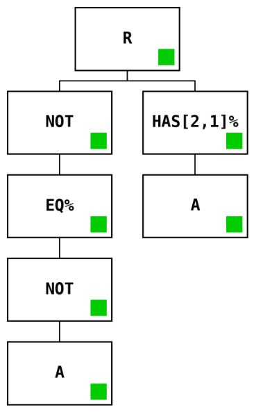
The not node is a special node that does not process the input string but rather toggles the accepted parity for its children. For example, regularly an s[1] node checks whether a string starts with a 1. However, when it is placed under a not node, it checks whether a string does not start with a 1. Figure 3 demonstrates the effect of not on an input set of binary strings that represent the concept of length being different than 3.
Starts With
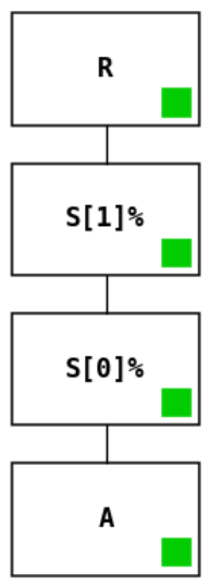
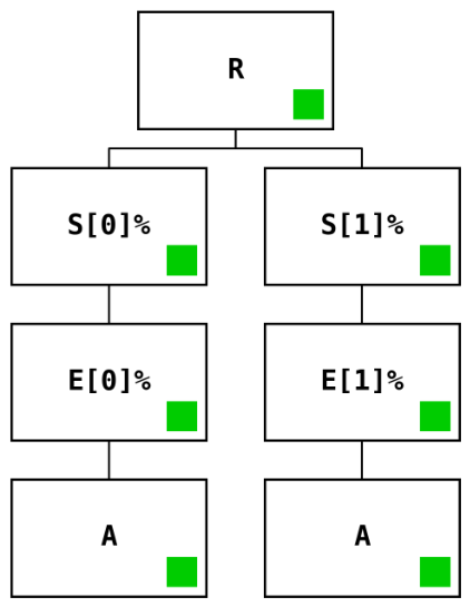
The s node represents the fundamental concept of starting with a specific character. The character is given as an argument, hence it has two versions: starts with 1 and starts with 0. Additionally it has trim and non-trim variants. The trim variant removes the heading character of the string upon a successful matching. Therefore, in a chain of starts with nodes one can check whether a string starts with longer sequences of characters. Figure 4 demonstrates the use of starts with nodes in a very simple example. Where the presented concept is strings that start with ‘10’, the obtained tree has a single path containing one s[1]% and one s[0]% node. Both nodes are used in their trim variants. Especially the s[1]% node has to be a trim variant so that the next node can check the second character of the string rather than re-checking the first character.
Ends With 
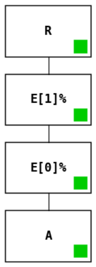
The e node represents the fundamental concept of ending with a specific character. This node is very similar to the starts with node, with the only difference being that it works from the end. It has trim and non-trim variants, where the trim variant removes the last character of the string upon a successful matching. Therefore, in a chain of ends with nodes one can check whether a string ends with longer sequences of characters. Figure 5 demonstrates the use of ends with nodes, where the presented concept is strings that end with ‘01’, the obtained tree has a single path containing one e[1]% and one e[0]% node. Both nodes are used in their trim variants. Especially the e[1]% node has to be a trim variant so that the next node can check the second to last character of the string rather than re-checking the last character.
Has    
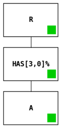
The has node checks whether the input string contains a given character ‘c’ for at least a certain number ‘n’ of times. For example, given the input string ‘10110’, has[3,0] rejects the string, whereas the input string ‘1001100’ is accepted by the same node. The has node has a trim and non-trim variant. Similar to the previous node types, the trim version removes all of the matching ‘c’ characters from the string, if there are at least ‘n’ of them. Figure 6 demonstrates the has[3,0] node case, which accepts all strings that have at least three 0 s.
Length    
The len node checks whether the input string is of a certain length ‘n’. For example, given the input string ‘10110’, len[3] rejects the string, whereas the input string ‘100’ is accepted by the same node. The len node has a trim and non-trim variant. The trim version simply removes all characters from the string. Figure 7 demonstrates the len[3] node case, which accepts all strings that have a length of 3.
Equals    
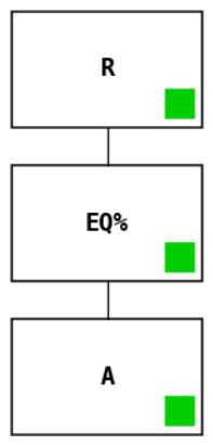
The EQ node checks whether the input string has the same number of 1 s and 0 s. For example, given the input string ‘10110’, eq rejects the string, whereas the input string ‘1001’ is accepted by the same node. The eq node has a trim and non-trim variant. The trim version simply removes all characters from the string. Figure 8 demonstrates the eq node case, which accepts all strings that have an equal number of ones and zeros.
The choice of these particular eight node types is deliberate but not claimed to be canonical: they were selected to cover, with a minimal vocabulary, the basic structural dimensions along which a short binary string can be characterized—positional information at the two ends (starts with, ends with), counting information (has, and the relational equal), size (length), and the logical operators needed to combine and close off rules (not, any), all anchored at the root. This set is intentionally small and, we stress, incomplete: many natural concepts (for example “contains the substring 101”) cannot be expressed with it. Enlarging the vocabulary would let CTL learn a much larger class of intermediate concepts, but at a steep computational price: as the complexity analysis in Section 4.2 makes precise, each additional atomic predicate (with its trim and non-trim variants) increases the branching factor P and therefore inflates the ( P L ) d search cost. We therefore deliberately restrict ourselves to this compact set, which is already expressive enough to capture a range of non-trivial intermediate concepts, as the experiments will show. In the next section, we explain how we query a concept tree to obtain the best concept definition.

3.3.4. Filtering a Tree

Once constructed with many inputs, the concept tree stores all kinds of rules (paths) to describe the inputs line by line. Unfortunately, these rules are mostly overlapping: two or more different rules can describe the same input line. Therefore, we have to filter the desired rules from the tree. Our aim here is twofold: pick as few rules as possible and as short rules as possible. We propose, in parallel to the classic Occam’s Razor principle, that the simplest answer is the best answer.
We formalize this filtering step as a weighted set-cover problem. Let Π = { π 1 , , π m } be the set of active leaf paths remaining after construction and destruction, and recall from Section 3.3.1 that each path π j accepts exactly the positive examples in S j = cov ( π j ) D + . By construction every active path is consistent, so S j D = for all j; the only remaining task is to cover the positives. We must therefore select a subfamily F Π such that
π j F S j = D + ,
i.e., every positive example is explained by at least one selected rule. Among all families satisfying (5) we seek the one minimizing a cost that encodes Occam’s Razor,
F = arg min F π j F 1 + λ depth ( π j ) ,
where the unit term penalizes the number of rules and the depth term breaks ties in favor of shorter rules. We take λ in the lexicographic limit λ 0 + , so that (6) is exactly the minimum-cardinality set-cover objective (minimize the number of selected paths) with total depth as a secondary, tie-breaking criterion; we do not tune λ as a free parameter. Minimum-cardinality set cover is NP-hard [36]; the universe to be covered is D + and the available sets are the S j . Note that overlap between rules ( S i S j ) is expected and harmless: it simply means a positive example admits several valid explanations, and the objective (6) resolves the redundancy by keeping the smallest covering subfamily.
Special cases fall out naturally. If some single path covers all of D + , then the optimum of (6) is that path alone (the shortest such, by the depth tie-break); only when no single rule suffices is a genuine disjunction of several paths selected. Because an exact solution is intractable, we approximate the cardinality objective with the classical greedy set-cover heuristic in the analysis of Lund and Yannakakis [37], which repeatedly selects the path of maximum marginal coverage. Concretely, each candidate path is scored by how many still-uncovered positives it covers, normalized by how many other active paths also cover those positives (so that rules covering “rare” positives are favored), and the depth tie-break of (6) is applied within this selection to prefer shorter paths; the chosen path’s covered positives are then removed from the universe and the process repeats. Formally, writing U D + for the set of positives not yet covered (initially U = D + ), each iteration selects
π = arg max π Π | cov ( π ) U | 1 + λ depth ( π ) , U U cov ( π ) ,
and halts when U = ; the denominator realizes the same depth tie-break as (6) (in the limit λ 0 + it reduces to plain maximum marginal coverage). For a universe of size | D + | , this greedy rule returns a cover of size at most H ( | D + | ) = k = 1 | D + | 1 k ln | D + | + 1 times the optimum [37], i.e., it targets the minimum-cardinality term of (6) with a logarithmic approximation factor rather than minimizing the depth-weighted sum exactly; the depth term enters only as a tie-break, which is adequate for the small rule families that arise in practice. The procedure interacts cleanly with the tree’s hierarchy: scoring and selection range over leaf paths, while the inheritance structure of the tree is used only to enumerate candidate paths and to read off each path’s predicate sequence.
Because the filtering step is an approximation, it is fair to ask whether the choice of heuristic risks selecting an incorrect or unnecessarily large rule set. Two observations bound this risk. First, the approximation only affects which minimal cover is reported, never correctness: every candidate path is, by construction, consistent with the data (it accepts all positives reaching it and no negative), so any selected subfamily that covers D + classifies the entire training set correctly regardless of the heuristic. The only quantity the heuristic can degrade is parsimony—in the worst case, it could return a cover up to a logarithmic factor larger than the optimum [37]. Second, we checked this empirically: re-running all 29 tasks with a simpler greedy maximum-coverage selection rule in place of the Lund–Yannakakis rule yielded the identical final rule set in every one of the 29 cases, with  100 % training accuracy throughout. For the small, low-overlap rule families that arise in this setting, the result is therefore insensitive to the particular approximation used; a systematic study of harder instances where the heuristics diverge is left to future work. We now continue with an example to demonstrate how our concept learner operates on a relatively complicated example.

3.4. Example Case

We now provide an example input and the state of the tree upon reading each line of the input to demonstrate how the overall operation works. The concept we will try to learn is to start and end with the same character. Clearly, once we learn this intermediate-level concept, we can use it to learn higher-level concepts such as a palindrome; however, that is a topic for our future studies. Let us call the concept of starting and ending with the same character as c. The input data provided to learn c is given in Table 3. The first 8 lines provide positive examples, whereas the next 6 are negative. Note that after reading the first 8 lines of input, the concept tree will already contain the desired answer. However, our algorithm is designed to respond with the simplest explanation possible, which in this case is to accept anything, upon reading the first 8 lines. Therefore, after reading the first 8 lines of input and processing them one by one the learned concept is simply a single any as shown in Figure 9.
Note that at this point the tree already contains thousands of nodes; however, we only display the response produced. The ninth line provides the first negative input to the algorithm. This negative input changes a lot of things, since many paths that are already deemed to be positive are now marked to be negative. Note that a path may match many positive input lines; however, matching a single negative input makes it negative. For example, our previous best response, the single any node, is not positive anymore. As a result, after reading the ninth line, our response changes to the concept tree shown in Figure 10.
Now, the simplest subtree that explains the first nine lines appears to be much more complicated. It consists of two distinct paths which hint at an “or” relation between them. The first path corresponds to “any string where the number of 1 s and 0 s are not equal”, whereas the second path corresponds to “any string containing at least two 1 s”. Note that the second not on the first path actually cancels the first not on the same path and allows any to operate as usual. In other words, the path should be understood as not[eq%-not[any]] and not as not[eq%]-not[any].
At this point we can see that the first path covers the positive input lines 1, 2, 4, 5, 6, and 8, whereas the second path covers positive lines 3, 5, 6, 7, and 8. Together, they cover all eight positive lines while correctly excluding the ninth (negative) line. As a result, the overall concept becomes “any string whose numbers of 1 s and 0 s differ, or which contains at least two 1 s”.
We now read the next line which is “001-”. Obviously, with our current best response, this line should be positive, as the “unequal counts” path covers it (“001” has two 0 s and one 1). However, it is provided to be negative. This again changes things in the tree, and the new response is given in Figure 11. As expected, the concept has changed drastically. The addition of the knowledge on the tenth line has invalidated the earlier assumptions and outlined an alternative concept definition. We still have two paths, but now one represents “strings ending with 0” and the other represents “strings containing at least two 1 s”. Simply put, the concept is now “strings ending with 0 or containing at least two 1 s”. When we compare the concept and the inputs, we see that the first four positive lines match the left path and the second four match the right path, whereas the ninth and tenth lines mismatch both paths, as expected.
The next line is another negative line: “0011-”. This line already matches the existing concept response, therefore does not cause any change in the response. However, the twelfth line is once again conflicting with our earlier assumptions and causes major changes in the response, shown in Figure 12. We now see that the response has two paths corresponding to strings “starting and ending with 1” or “starting and ending with 0”. Clearly, this was the concept we wanted the tree to learn. It took only twelve input lines to learn the concept; the thirteenth and fourteenth lines will not improve or change the response any further. An intriguing question is whether it was possible or not to teach this concept with even fewer input lines. Although we can answer this question for this specific concept through extensive trials, that is not a question which has a trivial answer when universally quantified. Finding the minimal training set for each intermediary concept is an obvious future research topic in this field.

4. Results and Discussion

We have done numerous tests on our CTL engine. We have observed that in all these tests, CTL was able to learn the desired concept in very limited input lines. Of course, our tests at this point do not involve complicated intermediate concepts. Considering that we are using only a very limited set of atomic concepts to learn intermediary concepts, we have confined ourselves to relatively simple scenarios, one of which was demonstrated in the previous section: the concept c of Section 3.4, namely “start and end with the same character” (the 14-line dataset of Table 3). For this specific example, we now want to present two important performance metrics: tree size and time spent. Figure 13 displays the growth speed of the concept tree as new lines of input are fed to the engine. Figure 14 shows the time spent for processing each input line.
When we consider the tree size growth plot, we can see that the growth speed decreases as new lines are processed. Once the concept is learned, the plot line almost flattens; for the example case, the tree stabilizes at roughly 6800 nodes. This behavior repeats in all the tests we have executed: the bulk of growth occurs while positive examples are ingested, after which the negative examples mostly prune rather than expand the structure. Clearly, if we were to allow more atomic concepts and deeper tree construction, the size of the tree would increase in response; these horizontal and vertical expansions are analyzed quantitatively in Section 4.2.
The processing time plot reports the mean and standard deviation of the per-line time over nine independent runs. Per-line processing is fast—on the order of a tenth of a second (mean 0.112  s, standard deviation 0.076  s for this example)—and, crucially, does not grow as the tree accumulates nodes: the lines processed last (the negative examples, when the tree is largest) are not slower than the early lines. Instead, the per-line cost tracks the input length: the tallest bars correspond to the longest input strings (the two length-five positives), and the final bar additionally absorbs the one-off set-cover filtering step. This is the expected behavior, because each new input line only affects a local neighborhood of the tree whose size is governed by the input length, the (constant) number of atomic concepts, and the (constant) allowed tree depth, rather than by the global tree size. We make this dependence precise in the complexity analysis below.
Together with this example case, we have done 28 more tests to observe the capabilities and performance metrics of CTL. In Table 4, we give a short summary of each test case. The ‘S (F)’ column represents the input size and the line of input after which the desired concept is found, the ‘T’ column represents the total elapsed learning time, the ‘Idea’ column is a very short summary of the concept being learned, the ‘Response’ column represents the corresponding tree paths, and the ‘Nodes’ column represents the total tree size. The responses are written in a normalized form, dropping the root prefix and any trailing vacuous accept-terminal (any, or a childless not, which behaves identically) for readability. We note that perfect training accuracy is not in itself an informative result here: by construction CTL only ever retains paths consistent with the data, so 100 % agreement with the training labels is guaranteed whenever a consistent rule exists in the hypothesis space. The meaningful questions are how few examples it needs and how well the learned rule generalizes, which we examine in Section 4.1. With that caveat, the table shows that in all but a few scenarios CTL converges to its final answer well before the last example is read (column F). Formally, writing Π ( D 1 : k ) for the rule set distilled from the first k examples, we define the convergence line as the earliest prefix beyond which the answer no longer changes,
F = min k : Π ( D 1 : j ) Π ( D ) for all j k ,
where ≡ denotes equality of the induced classifiers (Equation (4)); F | D | always, and  F < | D | indicates that the trailing examples were redundant. We highlight that, compared with an earlier fixed-bound implementation, the dynamic numeric bound of Section 3.3.2 reduces the final tree size by roughly a factor of three to twenty (final trees now contain between 838 and 10,331 nodes) while recovering the identical concepts, which is the single most effective mitigation of the combinatorial growth discussed in Section 4.2.
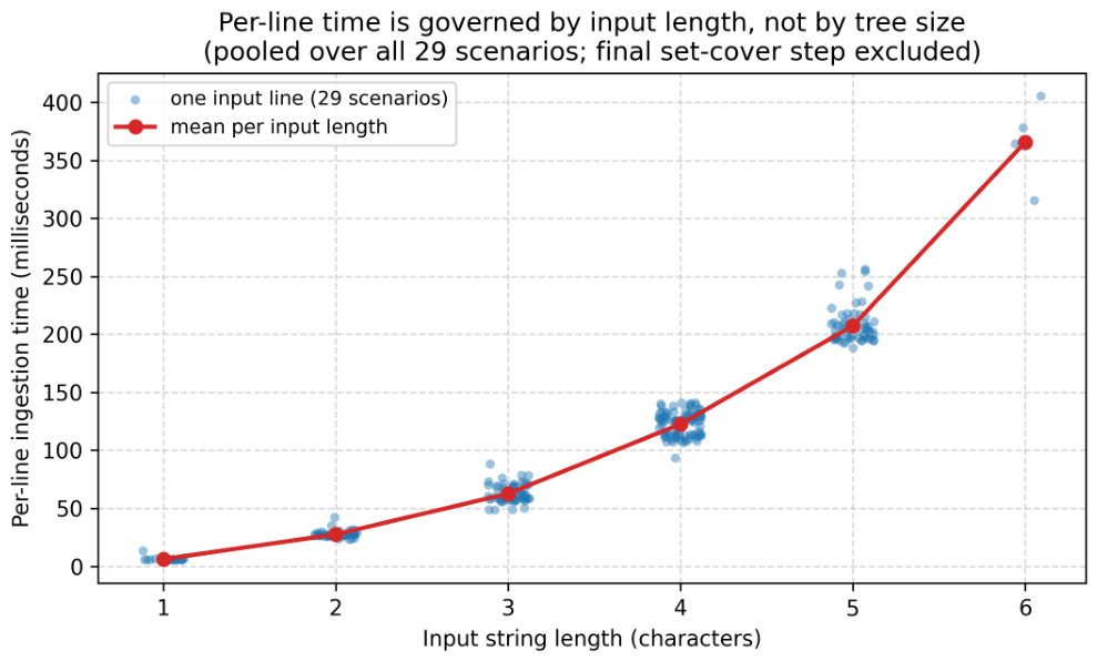
Figure 15 pools the per-line ingestion times of all 29 scenarios and plots them against the length of the input string processed on each line (the one-off final set-cover step of each scenario is excluded). The per-line cost is governed almost entirely by the input length: it rises smoothly from a few milliseconds for length-one strings to roughly 0.35 0.4  s for length-six strings, while the vertical spread at each length—reflecting different target concepts and different accumulated tree sizes—is comparatively small. In other words, neither the identity of the concept nor the size the tree has already reached is a major component of the per-line runtime. This is exactly the locality predicted by the complexity analysis of Section 4.2. Adding more atomic concepts or allowing deeper trees would increase this per-line cost, and we outline there concrete remedies—prioritized branch selection, depth pruning, and parallelization—for future, more demanding versions of CTL.
All experiments reported in this work were carried out on a single Apple-silicon workstation equipped with an Apple M4 system-on-chip (Apple Inc., Cupertino, CA, USA) (10 CPU cores, comprising 4 performance cores and 6 efficiency cores, arm64 architecture) and 16 GB of unified memory. The host operating system was macOS 26.3 (build 25D125). Wall-clock times were measured with Python 3.9.6’s high-resolution monotonic timer, and reflect single-threaded execution; no parallelization or GPU acceleration was employed.
The reference implementation is written in pure Python and was executed under CPython 3.9.6 inside an isolated virtual environment. Plotting utilities and numerical helpers rely on Matplotlib 3.9.4 (using the non-interactive Agg backend) and NumPy 2.0.2; the decision-tree baseline of Section 4.1 uses scikit-learn 1.6.1, and the RIPPER baseline uses the wittgenstein 0.3.5 package. Run-time figures correspond to the algorithmic stages only—tree initialization, per-line ingestion, and the final set-cover pruning step—and explicitly exclude all I/O and visualization costs (PNG rendering, on-disk artifact generation, convergence-line search, etc.), which are reported separately where relevant.

4.1. Comparison with Classical Symbolic Baselines

To position CTL against established symbolic learners, we compare it with two classical methods on all 29 datasets: a CART-style entropy decision tree—the ID3/C4.5 lineage [21,22] as implemented by scikit-learn’s DecisionTreeClassifier (criterion = entropy)—and ripper [38], a propositional rule learner. A fair comparison requires that all learners receive the same information, so we expose to both baselines exactly the atomic vocabulary that CTL uses, encoding each string as a feature vector of its atomic-predicate values: starts-with-0/1, ends-with-0/1, the counts of 0 s and 1 s, the length, and whether the two counts are equal. CTL composes these primitives into a concept tree; the decision tree splits on them; ripper forms a disjunctive rule set over them. We include ripper deliberately for two reasons: unlike a single axis-aligned tree, it natively expresses disjunctions, and so cannot be dismissed as disadvantaged on the “or”-concepts in our suite; and it is a modern representative of the covering-rule tradition that also includes CN2 [39] and, in the first-order setting, FOIL [26] (Section 2), so it stands in for that broader family of classical rule learners. All three learners are trained on the identical labeled datasets of Table 4. We do not include a few-shot large-language-model baseline as a table row, but recall that Figure 1 already provides a qualitative such comparison: three state-of-the-art LLMs fail to recover even the simplest of these patterns from the same handful of examples; a systematic quantitative LLM benchmark is left to future work.
We report generalization (accuracy against the intended concept over the exhaustive universe of all 126 binary strings of length 1 to 6, most of which are unseen during training), interpretability (the number of disjunctive rules, i.e., CTL leaf paths, CART leaves, or ripper clauses), and fit time. Restricting the test universe to length 6 is a practical choice; concepts that agree up to length six could in principle diverge at greater lengths, which we do not test. Table 5 summarizes the outcome over all 29 concepts and Table 6 gives the per-concept breakdown.
The picture is consistent and striking. Over all 29 concepts, CTL attains 95.5 % mean generalization accuracy ( 100 % on the 26 well-determined ones), against  72.1 % for the decision tree and 77.2 % for ripper, while expressing each concept with 1.3 rules on average versus 4.1 decision-tree leaves. Crucially, ripper—which can represent disjunctions and does so with a comparably small 1.4 rules—still falls well short of CTL, so CTL’s advantage is not merely an artifact of the decision tree’s inability to express “or”. The baselines degrade most on count-, length-, and suffix-based concepts (e.g., “at least four 0 s”, “ends with 00”): with only a few examples they latch onto spurious thresholds that do not extend to longer unseen strings, whereas CTL’s trimming-based composition captures the underlying structural rule exactly.
We are deliberately transparent about the three cases (datasets 1, 5, and 20, marked † in Table 6) where CTL scores below 100 % . In all three, CTL still classifies every training example correctly; the shortfall reflects under-determination of the dataset, not a learning error. Dataset 1 is the clearest illustration: its positives all have length three or four and its single negative has length five, so the data is equally consistent with “length is not five” and with “length is three or four”. The fixed-bound prototype happened to report the former; with the dynamic numeric bound, no length-five threshold is ever instantiated from the short positive examples, so CTL instead returns the equally valid “length three or four”, which disagrees with the nominal “not five” target on strings of other lengths. Dataset 5 is analogous: its three length-four positives (0011, 1010, 1100) all happen to contain exactly two 0 s, so “has at least two 0 s” (has[2,0]%) and “length four” both fit the data perfectly, and CTL returns the former. Dataset 20 (“same first and last character”) is similar: the learned two-predicate rule S [ c ] % E [ c ] % implicitly requires length at least two, so the single-character strings 0 and 1, absent from training, are missed. Such cases are a reminder that when a training set does not uniquely pin down a concept, CTL returns a simplest consistent rule, which need not be the one the dataset’s author had in mind; restricted to the 26 datasets whose training set does determine the target, CTL’s mean generalization is  100.0 % .
This accuracy comes at a computational price that we report honestly: CTL’s exhaustive search over consistent hypotheses takes a median of 1.39  s per dataset, against  0.56  ms for CART and 7.3  ms for ripper—three to four orders of magnitude slower. CTL therefore trades compute for sample efficiency and interpretability, a trade-off that is attractive in the few-example, interpretability-critical regime targeted here but that would need the optimizations of Section 4.2 for larger problems.
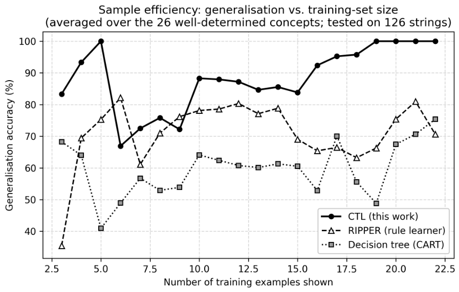
Figure 16 shows the advantage as a function of training-set size: CTL reaches near-perfect generalization almost immediately and stays there, while both baselines plateau well below it.

4.2. Computational Complexity and Scalability

We now analyze the cost of the procedure and explain the tree-growth behavior reported above. Let n be the number of training examples, L the maximum input length, P the number of atomic node types (here P = 8 ), and d the depth limit (MAX_LEVEL, here d = 4 ). At a single node processing a residual string of length L , construct considers each node type, each character argument ( | Σ | = 2 ), each numeric argument (bounded dynamically by ), and both trim variants, i.e., O ( P ) candidate children, each tested in O ( ) time. Expanding recursively to depth d, the number of nodes created while processing one example is bounded by the branching of feasible predicates raised to the depth, giving a worst-case per-example cost of
O ( P L ) d L ,
and the same expression bounds the per-example contribution to tree size. The total construction cost over a dataset is therefore O n ( P L ) d L and the worst-case tree size is O n ( P L ) d . Two facts make this tractable in practice. First, the exponent is the constant depth limit d, not the input length, so the cost is polynomial in L for fixed d; the apparent “explosion” is the ( P L ) d factor, controlled by capping d. Second, the dynamic numeric bound replaces a constant upper limit C by the residual length , and since shrinks with depth along trimming paths, the effective branching contracts as the recursion deepens.
The destruction pass is a single O ( tree size ) traversal per negative example. The final filtering step solves a set-cover instance whose universe is D + and whose sets are the active leaf paths; set cover is NP-hard [36], and we use the greedy O ( log | D + | ) -approximation [37], whose running time is polynomial in the number of active leaves and the number of positives—both small after pruning. Critically, the per-line analysis explains the flat timing curves of Figure 14 and Figure 15: a single example touches only the O ( ( P L ) d ) local neighborhood determined by its own length and the constant budgets P , d , independently of how many nodes the tree has already accumulated.
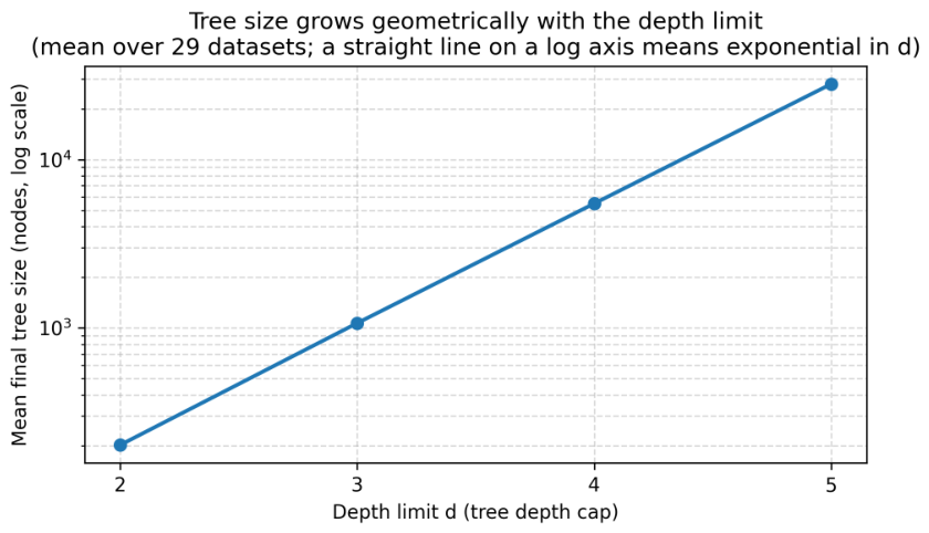
To make the dependence on d concrete rather than asymptotic, we ran the learner on all 29 datasets while varying only the depth limit d (Table 7, Figure 17). The mean final tree size grows by an almost constant multiplicative factor of 5.1 × for each unit increase in d ( 202 1069 5479 28,064 nodes for d = 2 , 3 , 4 , 5 ), which is the empirical signature of the geometric ( P L ) d bound and appears as a straight line on the log axis of Figure 17. Mean learning time grows in lockstep (from 14 ms at d = 2 to 13.6 s at d = 5 ). Crucially, the accuracy benefit saturates quickly: a depth of d = 3 already recovers the correct concept for 24 of the 29 tasks and d = 4 recovers all 29, so the depth used throughout this paper ( d = 4 ) sits exactly at the knee of the curve, buying full coverage before the cost escalates. This is direct evidence that the cap d—not the input length—is the lever that governs feasibility.
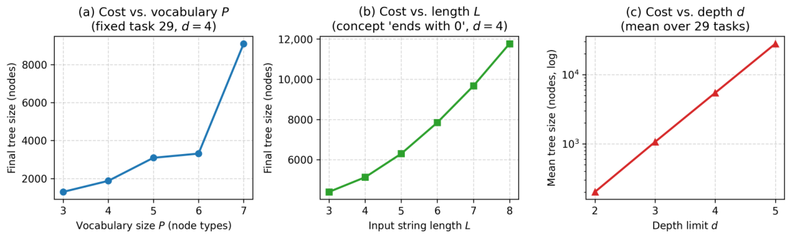
To isolate the contribution of each factor in the bound O n ( P L ) d , Figure 18 ablates the final tree size along all three hyperparameters independently. Panel (a) grows the set of atomic nodes P on a fixed task (number 29) by adding node types one at a time: the cost rises from 1300 nodes with only starts/ends/any to 9100 with the full set, with the largest jump caused by introducing not (which roughly doubles the admissible children at every node). Panel (b) grows the input length L for the fixed concept “ends with 0” at d = 4 : the cost rises smoothly and sub-exponentially (from 4400 nodes at L = 3 to 11,800 at L = 8 ), confirming the polynomial-in-L behavior predicted for fixed depth. Panel (c) reproduces the geometric growth in d from Table 7 on a log axis. Together, the three panels confirm that, of the three factors, the depth limit d is by far the dominant cost driver, while P and L contribute only polynomially at fixed depth.
These bounds also delineate where the prototype would struggle: longer inputs or a larger set of atomic nodes inflate the ( P L ) d factor, and a deeper d makes the dependence exponential in depth. Several standard remedies apply directly and are natural next steps: depth pruning and best-first heuristic search to avoid materializing the full breadth-first frontier, prioritized branch selection that expands only the most promising predicates, beam-style bounding of the number of live paths, and parallelization of the independent subtrees. We did not need these for the concepts studied here, but they are the obvious levers for scaling CTL to richer concept classes.

4.3. Limitations of the Current Framework

We close the discussion by stating the prototype’s limitations plainly, since several of them bound the claims above. (i) Binary, noise-free input. CTL currently operates only on strings over { 0 , 1 } and assumes that labels are correct; the destruct mechanism, which treats a single negative match as decisive, would need to be softened (for instance, with per-path penalty weights or statistical thresholds) before the method could tolerate label noise. (ii) Batch, sorted training. As established in Proposition 1, the safety of permanent deletion relies on processing all positive examples before any negative one; CTL is therefore a batch learner and does not yet support online or streaming data. An online variant would replace permanent deletion with reversible deactivation (which the implementation already distinguishes internally) and would re-expand a deactivated subtree when a later positive example demands a more specific descendant—precisely the specialization/refinement behavior that the deletion-based prototype achieves only by virtue of the sorted ordering. (iii) Fixed, incomplete predicate vocabulary. The eight atomic predicates cannot express many natural concepts; enlarging the vocabulary increases expressiveness but also the ( P L ) d search factor, and automatic predicate invention—discovering new atomic concepts from data, as opposed to selecting among given ones—remains open, as it does for much of inductive logic programming. (iv) Flat (non-hierarchical) concepts. The present learner induces a single concept; the envisioned reuse of a learned concept as an atomic predicate in a higher-level learner is not yet implemented. (v) Narrow data and task scope. Our evaluation is confined to short, noise-free binary strings and to concepts expressible as syntactic string patterns; we do not study multi-character alphabets, continuous or real-valued attributes, or genuinely multimodal data (images, text), nor fuzzy concepts, noisy labels, or open-ended concept generation. The 29 tasks therefore probe the mechanics of the learner rather than general-purpose concept learning, and the gap between this controlled setting and broad, human-level generalization should not be understated. Extending the predicate vocabulary to multi-character alphabets and adding a noise model are the natural first steps toward a less restricted evaluation. (vi) Single-machine, serial measurement. All timings are from a single Apple-silicon workstation running single-threaded CPython; we do not report cross-hardware results, parallel or GPU acceleration, or stress tests at large data volumes. The complexity analysis of Section 4.2 characterizes the asymptotics, but absolute runtimes on other platforms, and the constant factors achievable with the optimizations listed there, remain to be measured. (vii) Dependence on negative examples; over-generalization risk. Because CTL specializes a concept only in response to negative examples, a training set with too few negatives can leave the concept under-constrained, yielding an over-general rule. In the extreme, given only positive examples the simplest consistent hypothesis is the trivial any rule, which CTL duly returns (Figure 9); the under-determined datasets of Section 4.1 are milder instances of the same effect. The method therefore presupposes a training set whose negatives sufficiently delimit the concept boundary. Quantifying rule reliability under limited data—for example with a held-out validation set or a Minimum Description Length criterion that trades rule complexity against coverage—is a useful safeguard we leave to future work. We regard (ii)–(vii) less as defects than as a concrete research agenda, and we return to them in the conclusion.

5. Conclusions

This paper introduced the Concept Tree Learner (CTL), a novel approach to machine learning that departs fundamentally from the statistical paradigm dominating modern AI. Rather than learning from massive corpora of text or data, CTL learns concepts incrementally from a small number of labeled binary string examples, building an interpretable tree structure that encodes logical rules composable from a fixed set of atomic operations.
Our experiments across 29 test cases demonstrate that CTL fits every training set exactly (consistency is guaranteed by construction) and recovers the intended target concept on the 26 tasks whose data uniquely determines it—returning a different but data-consistent rule on the remaining three—often converging well before all training examples are exhausted. The engine correctly learned a range of concepts—from simple atomic patterns like “starts with 1” or “ends with 0”, to compound disjunctions and conjunctions such as “starts and ends with the same character”—using only eight node types and modest depth limits. On a shared atomic vocabulary and across all 29 tasks, CTL generalized to unseen strings far better than both a classical entropy decision tree and the RIPPER rule learner ( 95.5 % mean accuracy— 100 % on the 26 tasks whose training set determines the target—versus 72.1 % and 77.2 % ), while using fewer and shorter rules ( 1.3 on average against 4.1 decision-tree leaves), underscoring its sample efficiency and interpretability. Per-line processing time stayed low (a few tens of milliseconds) and, as our complexity analysis predicts, depended on input length rather than on the accumulated tree size; the dynamic predicate-argument bound further kept final trees an order of magnitude smaller than a fixed-bound implementation while recovering the identical concepts. Tree growth decelerates once a concept is learned, hinting at an inherent regularization property of the approach.
Critically, CTL’s outputs are not black-box predictions but human-readable rule sets. Every classification decision can be traced to an explicit path in the concept tree, making the system fully transparent and verifiable. Each path moreover maps directly onto a natural-language sentence: the rule s[1]% e[0]%, for instance, reads as “the string starts with a 1 and, after that 1 is removed, ends with a 0”, and the three-way disjunction of Table 4 (row 29) reads as “a 4-bit string ending in 0, or a 5-bit string ending in 1, or any 3-bit string”. A lightweight module that emits such glosses automatically would further improve accessibility for non-specialist readers and is a natural, low-risk addition. This places CTL squarely within the agenda of interpretable and explainable AI [27], and contrasts with deep models that offer no comparable account of their decisions.
That said, the current implementation carries important limitations. The atomic node set is fixed and demonstrably incomplete: many concepts that a human would find natural cannot be expressed with the eight node types available. The system also operates only on binary strings and assumes noise-free input, constraints that would need to be relaxed for any real-world deployment. Computational cost grows with the number of atomic concepts and tree depth, and the set cover filtering step is an NP-hard problem solved only approximately.
These limitations, however, are not fundamental objections to the approach—they are a research agenda. The path forward includes expanding the atomic concept vocabulary, developing mechanisms for automatic node type discovery, extending CTL to multi-character alphabets, and introducing robustness to noisy data. Ultimately, the most ambitious direction is hierarchical concept composition: using concepts learned by one CTL instance as atomic building blocks for a higher-level instance, mirroring the layered way human cognition builds understanding from simple percepts to complex abstractions.
In summary, CTL is a principled and rigorously evaluated base learner for interpretable symbolic concept induction. It demonstrates that concept-level, logic-grounded, bottom-up learning over binary strings is computationally feasible, sample-efficient, and fully interpretable, and that it can outperform a classical decision-tree learner on the same vocabulary in both generalization and rule compactness. We see it as a modest but concrete building block: as the predicate vocabulary is enriched and learned concepts are composed hierarchically, such structured symbolic learners may complement the prevailing statistical methods on the long road toward more general and genuinely explainable artificial intelligence.

Author Contributions

Conceptualization, M.T.E. and B.G.; Methodology, M.T.E. and B.G.; Software, M.T.E.; Resources, B.G.; Writing—original draft, M.T.E. and B.G.; Writing—review & editing, B.G.; Visualization, M.T.E.; Supervision, B.G.; Project administration, B.G. All authors have read and agreed to the published version of the manuscript.

Funding

This research received no external funding.

Institutional Review Board Statement

Not applicable.

Informed Consent Statement

Not applicable.

Data Availability Statement

The data and source code supporting the findings of this study are publicly available in Zenodo at https://doi.org/10.5281/zenodo.20384747.

Conflicts of Interest

The authors declare no conflicts of interest.

References

  1. Russell, S.; Norvig, P.; Popineau, F.; Miclet, L.; Cadet, C. Intelligence Artificielle: Une Approche Moderne, 4th ed.; Pearson France: Paris, France, 2021. [Google Scholar]
  2. Goertzel, B. Artificial general intelligence: Concept, state of the art, and future prospects. J. Artif. Gen. Intell. 2014, 5, 1. [Google Scholar] [CrossRef] [Scilit]
  3. Lake, B.M.; Ullman, T.D.; Tenenbaum, J.B.; Gershman, S.J. Building machines that learn and think like people. Behav. Brain Sci. 2017, 40, e253. [Google Scholar] [CrossRef] [Scilit] [PubMed]
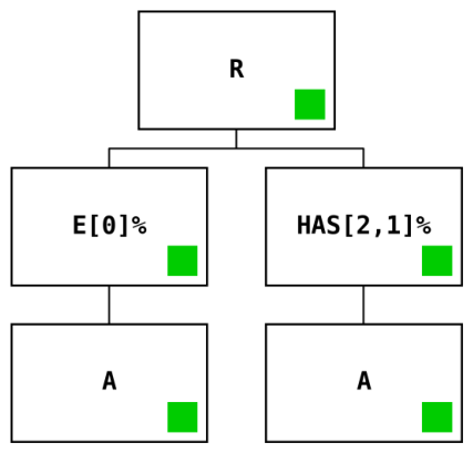
  4. Bubeck, S.; Chandrasekaran, V.; Eldan, R.; Gehrke, J.; Horvitz, E.; Kamar, E.; Lee, P.; Lee, Y.T.; Li, Y.; Lundberg, S.; et al. Sparks of artificial general intelligence: Early experiments with gpt-4. arXiv 2023, arXiv:2303.12712. [Google Scholar]
  5. Tenenbaum, J.B.; Kemp, C.; Griffiths, T.L.; Goodman, N.D. How to grow a mind: Statistics, structure, and abstraction. Science 2011, 331, 1279–1285. [Google Scholar] [CrossRef] [Scilit] [PubMed]
  6. Bikkasani, D.C. Navigating artificial general intelligence (AGI): Societal implications, ethical considerations, and governance strategies. AI Ethics 2025, 5, 2021–2036. [Google Scholar] [CrossRef] [Scilit]
  7. Sonko, S.; Adewusi, A.O.; Obi, O.C.; Onwusinkwue, S.; Atadoga, A. A critical review towards artificial general intelligence: Challenges, ethical considerations, and the path forward. World J. Adv. Res. Rev. 2024, 21, 1262–1268. [Google Scholar] [CrossRef] [Scilit]
  8. Baum, S. A survey of artificial general intelligence projects for ethics, risk, and policy. SSRN 2017. [Google Scholar] [CrossRef] [Scilit]
  9. Buttazzo, G. Rise of artificial general intelligence: Risks and opportunities. Front. Artif. Intell. 2023, 6, 1226990. [Google Scholar] [CrossRef] [Scilit] [PubMed]
  10. Emmert-Streib, F. Is ChatGPT the way toward artificial general intelligence. Discov. Artif. Intell. 2024, 4, 32. [Google Scholar] [CrossRef] [Scilit]
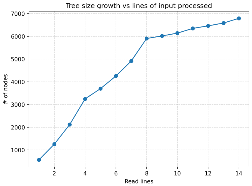
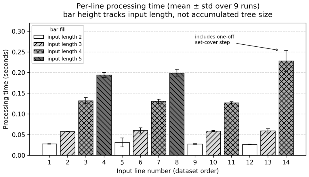
  11. Mumuni, A.; Mumuni, F. Large language models for artificial general intelligence (AGI): A survey of foundational principles and approaches. arXiv 2025, arXiv:2501.03151. [Google Scholar]
  12. Ge, Y.; Hua, W.; Mei, K.; Ji, J.; Tan, J.; Xu, S.; Li, Z.; Zhang, Y. Openagi: When llm meets domain experts. Adv. Neural Inf. Process. Syst. 2023, 36, 5539–5568. [Google Scholar] [CrossRef] [Scilit]
  13. Javaid, S.; Khan, N.; Alwarafy, A.; Saeed, N. AGI and LLM-Driven Spectrum Intelligence in Future Wireless Networks. IEEE Wirel. Commun. 2025, 33, 224–233. [Google Scholar] [CrossRef] [Scilit]
  14. Joshi, S. Review of Artificial General Intelligence (AGI): Implications for the US Workforce and Economic Stability. Int. J. Innov. Sci. Eng. Manag. 2025, 4, 336–350. [Google Scholar] [CrossRef] [Scilit]
  15. Korinek, A.; Suh, D. Scenarios for the Transition to AGI; Technical Report; National Bureau of Economic Research: Cambridge, MA, USA, 2024. [Google Scholar]
  16. Krause, D. The Impending Disruption: The Transformative Effects of Artificial General Intelligence on Employment in Financial Services. SSRN 2025. [Google Scholar] [CrossRef] [Scilit]
  17. Bara, M. Moravec’s Paradox and Restrepo’s Model: Limits of AGI Automation in Growth. arXiv 2025, arXiv:2509.24466. [Google Scholar]
  18. Yao, H.; Huang, J.; Qiu, Y.; Chen, M.K.; Liu, W.; Zhang, W.; Zeng, W.; Zhang, X.; Zhang, J.; Song, Y.; et al. MMReason: An Open-Ended Multi-Modal Multi-Step Reasoning Benchmark for MLLMs Toward AGI. arXiv 2025, arXiv:2506.23563. [Google Scholar]
  19. Potapov, A.; Svitenkov, A.; Vinogradov, Y. Differences between Kolmogorov complexity and Solomonoff probability: Consequences for AGI. In Proceedings of the International Conference on Artificial General Intelligence, Oxford, UK, 8–11 December 2012; pp. 252–261. [Google Scholar]
  20. Yue, X.; Ni, Y.; Zhang, K.; Zheng, T.; Liu, R.; Zhang, G.; Stevens, S.; Jiang, D.; Ren, W.; Sun, Y.; et al. MMMU: A massive multi-discipline multimodal understanding and reasoning benchmark for expert AGI. In Proceedings of the IEEE/CVF Conference on Computer Vision and Pattern Recognition, Seattle, WA, USA, 16–22 June 2024; pp. 9556–9567. [Google Scholar]
  21. Quinlan, J.R. Induction of decision trees. Mach. Learn. 1986, 1, 81–106. [Google Scholar] [CrossRef] [Scilit]
  22. Quinlan, J.R. C4.5: Programs for Machine Learning; Morgan Kaufmann: San Mateo, CA, USA, 1993. [Google Scholar]
  23. Breiman, L.; Friedman, J.H.; Olshen, R.A.; Stone, C.J. Classification and Regression Trees; Wadsworth: Belmont, CA, USA, 1984. [Google Scholar]
  24. Muggleton, S. Inductive logic programming. New Gener. Comput. 1991, 8, 295–318. [Google Scholar] [CrossRef] [Scilit]
  25. Cropper, A.; Dumančić, S.; Evans, R.; Muggleton, S.H. Inductive logic programming at 30. Mach. Learn. 2022, 111, 147–172. [Google Scholar] [CrossRef] [Scilit]
  26. Quinlan, J.R. Learning logical definitions from relations. Mach. Learn. 1990, 5, 239–266. [Google Scholar] [CrossRef] [Scilit]
  27. Rudin, C. Stop explaining black box machine learning models for high stakes decisions and use interpretable models instead. Nat. Mach. Intell. 2019, 1, 206–215. [Google Scholar] [CrossRef] [Scilit] [PubMed]
  28. Chen, L.; Lu, K.; Rajeswaran, A.; Lee, K.; Grover, A.; Laskin, M.; Abbeel, P.; Srinivas, A.; Mordatch, I. Decision transformer: Reinforcement learning via sequence modeling. Adv. Neural Inf. Process. Syst. 2021, 34, 15084–15097. [Google Scholar]
  29. Zitkovich, B.; Yu, T.; Xu, S.; Xu, P.; Xiao, T.; Xia, F.; Wu, J.; Wohlhart, P.; Welker, S.; Wahid, A.; et al. Rt-2: Vision-language-action models transfer web knowledge to robotic control. In Proceedings of the Conference on Robot Learning, Atlanta, GA, USA, 6–9 November 2023; pp. 2165–2183. [Google Scholar]
  30. Jiang, Z.; Yang, M.; Tsirlin, M.; Tang, R.; Dai, Y.; Lin, J. “Low-resource” text classification: A parameter-free classification method with compressors. In Proceedings of the Findings of the Association for Computational Linguistics: ACL 2023, Toronto, ON, Canada, 9–14 July 2023; pp. 6810–6828. [Google Scholar]
  31. Shi, Y.; Yuan, L.; Chen, Y.; Feng, J. Continual learning via bit-level information preserving. In Proceedings of the IEEE/CVF conference on Computer Vision and Pattern Recognition, Virtual, 19–25 June 2021; pp. 16674–16683. [Google Scholar]
  32. HANS, J. A Hybrid Cognitive Architecture for AGI: Bridging Symbolic and Subsymbolic AI. Int. J. Multidiscip. Res. 2025, 7, 1–4. [Google Scholar]
  33. Dhadi, S.P.R.; Biradar, A.; Maram, M.R.; Gundu, S.; Mididuddi, D.; Burra, S. Redefining AGI: The First Practical Framework and Working Demo of General Intelligence. Preprint 2025. [Google Scholar] [CrossRef] [Scilit]
  34. Ibarz, B.; Kurin, V.; Papamakarios, G.; Nikiforou, K.; Bennani, M.; Csordás, R.; Dudzik, A.J.; Bošnjak, M.; Vitvitskyi, A.; Rubanova, Y.; et al. A generalist neural algorithmic learner. In Proceedings of the Learning on Graphs Conference, Virtual, 9–12 December 2022; pp. 1–23. [Google Scholar]
  35. Reed, S.; Zolna, K.; Parisotto, E.; Colmenarejo, S.G.; Novikov, A.; Barth-Maron, G.; Gimenez, M.; Sulsky, Y.; Kay, J.; Springenberg, J.T.; et al. A generalist agent. arXiv 2022, arXiv:2205.06175. [Google Scholar]
  36. Edmonds, J.; Karp, R.M. Theoretical improvements in algorithmic efficiency for network flow problems. J. ACM (JACM) 1972, 19, 248–264. [Google Scholar] [CrossRef] [Scilit]
  37. Lund, C.; Yannakakis, M. On the hardness of approximating minimization problems. J. ACM (JACM) 1994, 41, 960–981. [Google Scholar] [CrossRef] [Scilit]
  38. Cohen, W.W. Fast effective rule induction. In Proceedings of the Twelfth International Conference on Machine Learning (ICML), Tahoe City, CA, UAS, 9–12 July 1995; pp. 115–123. [Google Scholar]
  39. Clark, P.; Niblett, T. The CN2 induction algorithm. Mach. Learn. 1989, 3, 261–283. [Google Scholar] [CrossRef] [Scilit]
Figure 1. Three major large language models (LLMs)—Gemini, ChatGPT, DeepSeek—fail to recognize a simple pattern. The responses shown were collected in February 2026 from the then-current public versions of the three models.
Applsci 16 08542 g001
Figure 2. An example tree with two rules identified.
Applsci 16 08542 g002
Figure 3. The Not node negates the polarity of its children.
Applsci 16 08542 g003
Figure 4. The Starts With node checks whether a string starts with the given character.
Applsci 16 08542 g004
Figure 5. The Ends With node checks whether a string ends with the given character.
Applsci 16 08542 g005
Figure 6. The Has node checks whether a string contains a specific character at least a specific number of times.
Applsci 16 08542 g006
Figure 7. The Len node checks whether a string is of a certain length.
Applsci 16 08542 g007
Figure 8. The Equals node checks whether a string has the same number of 1 s and 0 s.
Applsci 16 08542 g008
Figure 9. The concept learned after processing the first eight lines of input.
Applsci 16 08542 g009
Figure 10. The ninth line is negative and causes a drastic change in the tree.
Applsci 16 08542 g010
Figure 11. The tenth line further shapes the response.
Applsci 16 08542 g011
Figure 12. The twelfth line further shapes the response.
Applsci 16 08542 g012
Figure 13. Tree size growth versus number of input lines processed, for the example case (concept c: “start and end with the same character”; the 14-line dataset of Table 3). Growth is rapid while the eight positive examples are ingested and then quickly slows down.
Applsci 16 08542 g013
Figure 14. Per-line processing time for the example case (concept c: “start and end with the same character”; mean ± standard deviation over nine runs). Bars are shaded and hatched by the length of the input string processed on that line: the height tracks the input length, not the accumulated tree size (e.g., lines 9–14, processed when the tree is largest, are no slower than the early lines). The final bar additionally includes the one-off set-cover filtering step.
Applsci 16 08542 g014
Figure 15. Per-line ingestion time as a function of input string length, pooled over all 29 scenarios (each point is one input line; the one-off final set-cover step of each scenario is excluded). The per-line cost grows with the input length and is essentially independent of which concept is being learned or of the accumulated tree size, consistent with the locality argument of the complexity analysis (Section 4.2).
Applsci 16 08542 g015
Figure 16. Sample efficiency. Generalization accuracy is the fraction of the 126 binary strings of length 1–6 that a learner labels in agreement with the intended concept; most are never shown during training. Curves are averaged over the 26 well-determined concepts, excluding the three under-determined datasets of Table 6. On the same atomic features, CTL reaches near-perfect generalization almost immediately, whereas ripper and the entropy decision tree plateau far below.
Applsci 16 08542 g016
Figure 17. Mean final tree size (over all 29 datasets) versus the depth limit d, on a logarithmic vertical axis. The near-straight line confirms that tree size grows geometrically in d, consistent with the ( P L ) d worst-case bound; the depth used in this paper ( d = 4 ) is the smallest that recovers every target concept.
Applsci 16 08542 g017
Figure 18. Ablation of cost (final tree size) along the three hyperparameters of the bound O n ( P L ) d : (a) number of atomic nodes P, (b) input string length L, and (c) depth limit d (log axis). Each is varied with the others held fixed. Cost grows polynomially with P and L but geometrically with d.
Applsci 16 08542 g018
Table 1. An example dataset of “evenness” concept.
Binary StringClass
0+
1
10+
11
100+
101
110+
111
1000+
1001
1010+
Table 2. Eight different node types along with their short description.
Name(Symbol)CharNumDescription
Root(r)NoNoFirst node of any concept tree
Any(a)NoNoAccepts any string, ends a path
Not(not)NoNoNegates its child path’s value
Starts with(s)YesNoTrue if input starts with given character
Ends with(e)YesNoTrue if input ends with given character
Has(has)YesYesTrue if input has given number of given character
Length(len)NoYesTrue if input is of given length
Equal(equal)NoNoTrue if input contains equal amount of 0 s and 1 s
Table 3. Input file content for c.
IndexBinary StringConcept Polarity
100+
2010+
30110+
400100+
511+
6101+
71001+
811011+
901
10001
110011
1210
13110
141100
Table 4. Summary of test results for 29 test scenarios (dynamic-bound implementation). Every scenario is classified with 100 % training accuracy. Reported times are means over three runs on the workstation described at the end of this section; run-to-run variation is small (mean relative standard deviation 5 % ). In the Response column, a ‘%’ suffix denotes the trim variant of a node (Section 3.3.3); ‘→’ chains a node to its child along a path (logical AND under progressive trimming); and ‘∨’ separates the disjuncts of the final rule set.
iS (F)T (s)IdeaResponseNodes
15 (5)0.679Length three or four (disjunction)LEN[3]% ∨ LEN[4]%5416
24 (3)0.068Atomic starts-with-1 conceptS[1]%838
34 (3)0.068Atomic ends-with-0 conceptE[0]%838
45 (5)0.386At-least-three ones thresholdHAS[3,1]%2927
55 (4)0.726Exact length four (learns ≥ 2 zeros)HAS[2,0]%5617
65 (4)0.272Equal zeros and onesEQ%3122
75 (4)0.361Length-not-three via NOT nodeNOT→LEN[3]%3879
85 (5)0.202Chained starts-with prefix 10S[1]%→S[0]%2120
95 (4)0.247Chained ends-with suffix 01E[1]%→E[0]%2536
105 (4)0.672At-least-four zeros thresholdHAS[4,0]%4926
1110 (9)0.594Disjunction starts-1 or ends-0S[1]% ∨ E[0]%4229
1211 (10)2.180Length disjunction three or fiveLEN[3]% ∨ LEN[5]%10,331
1312 (8)0.752Prefix 00 via chained starts-withS[0]%→S[0]%4138
1412 (11)0.765Suffix 11 via chained ends-withE[1]%→E[1]%4761
1511 (7)1.508Conjunction count and endingE[0]%→HAS[3,1]%6353
1612 (10)1.498Prefix-zero and length-four conjunctionS[0]%→LEN[3]%6803
1713 (11)1.136Disjunction of two conjunctionsS[1]%→E[0]% ∨ S[0]%→HAS[3,1]%6298
1813 (10)0.845Position-or-length disjunctionS[1]% ∨ LEN[3]%4895
1913 (10)1.206Disjunction over count thresholdsHAS[3,1]% ∨ HAS[3,0]%6359
2014 (12)1.292Endpoint-equality palindrome-like symmetryS[0]%→E[0]% ∨ S[1]%→E[1]%6790
2115 (13)1.555Multiples of four (binary)E[0]%→E[0]%5312
2216 (9)2.039Multiples of eight (binary)E[0]%→E[0]%→E[0]%5610
2315 (5)1.582Four-divides not eight-dividesE[0]%→E[0]%→E[1]%4800
2414 (10)2.268Five-bit even numbersE[0]%→LEN[4]%9459
2517 (13)1.979Four-bit range eight to fifteenS[1]%→LEN[3]%8535
2615 (13)2.443Five-bit packet header patternS[1]%→E[0]%→LEN[3]%8347
2718 (17)1.937Positive multiples of fourS[1]%→E[0]%→E[0]%6245
2819 (18)2.598Multiple-of-four or odd 5-bitE[0]%→E[0]% ∨ E[1]%→LEN[4]%8309
2922 (19)2.937Three-tier ID classificationE[0]%→LEN[3]% ∨ E[1]%→LEN[4]% ∨ LEN[3]%9100
Table 5. CTL versus two classical symbolic learners on the same atomic-predicate vocabulary, summarized over all 29 concepts. Generalization is accuracy against the intended concept over all 126 strings of length 1–6; “Rules” counts CTL leaf paths, CART leaves, and ripper clauses. ripper natively expresses disjunctions, so unlike a single CART tree, it is not penalized on “or”-concepts, yet it still trails CTL substantially. Values are mean ± standard deviation across concepts.
LearnerGen. Acc. (All 29)Gen. Acc. (Well-Det., n = 26 )RulesTrain Acc.Median Fit Time
CTL (this work) 95.5 ± 16.6 % 100.0 % 1.3 ± 0.5 100.0%1386 ms
Decision tree (CART, entropy) 72.1 ± 24.2 % 72.9 % 4.1 ± 2.3 98.3%0.56 ms
ripper (rule learner) 77.2 ± 18.7 % 77.7 % 1.4 ± 0.5 87.8%7.28 ms
Table 6. Per-concept generalization accuracy (%) and rule count for all 29 concepts. marks the three datasets whose training set does not uniquely determine the target concept; there CTL still classifies every training example correctly but its simplest consistent rule differs from the nominal target. “Gen” is generalization accuracy; “R” is rule count.
iConceptnCTLCARTripper
Gen R Gen R Gen R
1Length not five 5442492501
2Starts with 14100110021001
3Ends with 0410011002511
4At least three 1 s51001562771
5Length exactly 4 5261752691
6Equal 0 s and 1 s5100110021001
7Length not three51001183291
8Prefix 1051001283721
9Suffix 0151001293671
10At least four 0 s51001342941
11Starts1 or ends010100210031002
12Length 3 or 51110029541002
13Prefix 00121001837791
14Suffix 11121001793751
15Three 1 s and ends 01110011003791
16Starts 0 and length 41210016051001
17(S1 & E0) or (S0 & 3ones)131002565752
18Starts 1 or length 313100210041002
193 zeros or 3 ones131002793542
20Same first and last 1498271111002
21Ends 00 (mult 4)151001593751
22Ends 000 (mult 8)161001674792
23Ends 100 (4 not 8)151001705671
24Even and length 51410016751001
25Starts 1 and length 41710011004762
26S1 & E0 & length 51510011005871
27S1 and ends 00181001834482
28Ends00 or (E1 & len5)191002569672
293-tier ID221003759712
Table 7. Empirical effect of the depth limit d on cost, averaged over all 29 datasets. Mean tree size grows by a roughly constant factor ( 5.1 × ) per unit depth—the empirical signature of the ( P L ) d bound—while d = 4 already recovers every target concept (column “Recovered”). The paper uses d = 4 ; d = 6 is omitted as its blow-up makes it impractical, which is itself the point.
dMean NodesMax NodesMean Time (s)Recovered
22022950.01411/29
3106917420.12424/29
4547910,3311.24529/29
528,06461,38313.56428/29
Disclaimer/Publisher’s Note: The statements, opinions and data contained in all publications are solely those of the individual author(s) and contributor(s) and not of MDPI and/or the editor(s). MDPI and/or the editor(s) disclaim responsibility for any injury to people or property resulting from any ideas, methods, instructions or products referred to in the content.