A Federated Learning and Knowledge Distillation-Based Load Identification Algorithm Under Heterogeneous Model Condition

Abstract

With the development of power system intelligence and information, load identification technology has played an important role in smart electricity utilization. Although traditional centralized load identification methods can improve model accuracy, they inevitably lead to increased risks of privacy leakage and high communication costs. In order to cope with the challenges of data privacy protection, model heterogeneity, and communication efficiency in the field of load identification, a federated learning (FL)- and knowledge distillation-based load classification algorithm under heterogeneous models is proposed in this paper. First, the measurement is transformed into an RGB image using Markov random fields, which not only provides more information but also satisfies the requirement of deep networks, so the actual load identification problem is formulated as an image classification problem. Then, the proposed FL framework is described. Each client uses different image classification networks for identification with its own computing power and requirements. In local training, the fine-tuning strategy is used where the parameters of feature extraction are frozen and only the classification parameters are trained. By introducing public data as a distillation carrier, each client can generate soft labels of the public dataset to represent the knowledge of their own data. At the server, knowledge sharing between datasets is achieved through aggregation. Both the soft labels and the trained parameters are aggregated by their corresponding the training performance. The proposed algorithm only transmits soft labels and classification parameters, which can ensure user privacy and reduce communication traffic. The experimental results demonstrate that the proposed algorithm improves the load identification performance under the WHITED and PLAID dataset conditions, compared with some existing methods.

1. Introduction

With the rapid development of intelligence and information in power systems, load identification has received much attention in smart power consumption, load management, and demand response. Accurate load identification not only enhances the operational efficiency of distribution networks but also provides end-users with energy efficiency analysis, fault diagnosis, and personalized energy services [1]. In applying smart meters and distributed energy resources, accurately identifying the type of electrical load from complex load data becomes a critical challenge in smart grid and smart energy management [2].

Traditional load identification methods heavily rely on centralized data collection and modeling. Moreover, the collected data from various power consumption terminals are uploaded to a central server for training. In presenting a non-intrusive load monitoring (NILM) method, the authors of [3] pointed out that this centralized paradigm is prone to data privacy concerns and data silos. It not only incurs high communication costs for massive data transmission but also limits fault tolerance and flexibility [4]. Consequently, in sensitive power consumption data environments, data owners are reluctant to share raw data directly due to privacy protection. Thus, efficient and secure collaborative modeling for offline training is an urgent challenge to be solved.

In recent years, federated learning (FL) has emerged as a research hotspot in load identification to resolve this data privacy issue. It enables collaborative training to derive a global model without centralizing raw data. Instead, participating parties only share model parameters or gradients to effectively protect data privacy [5]. Google demonstrated that local clients can upload model parameters to the Android cloud, while continuously downloading a public model from the cloud to enhance local model capabilities [6]. Kim proposed a consensus mechanism to exchange and verify local model updates when local data is decentralized [7]. Smith et al. [8] introduced multi-task federated learning where multiple clients are allowed to collaborate on the tasks.

Although techniques for FL-based load identification have been proposed in previous studies, they do not consider practical scenarios. The FedAvg-based load identification framework proposed in [9] failed to account for the non-independent and identically distributed (non-IID) characteristics of data. The federated load monitoring system designed by [10] adopts a model parameter aggregation strategy with fixed weights without considering the heterogeneity among edge terminals. This caused lagging model updates from resource-constrained clients, which in turn slowed down global model convergence and significantly increased identification errors. Furthermore, the FedAvg algorithm within FL frameworks mandates that all clients utilize homogeneous models, which is difficult to satisfy in practical environments with diverse terminals and hardware. In actual environments, different clients may employ different deep learning networks for training. Therefore, in this study, the problem of federated learning-based load identification under model heterogeneity constraints is investigated.

Recently, a knowledge distillation (KD) technique was used in the framework of federated learning to solve the constraints of model homogeneity. As a knowledge transfer technique, KD enables lightweight deployment and performance enhancement by training a smaller model (the student model) to minimize the output probability distribution of a larger model (the teacher model). With the KD, a physical teacher model is no longer required, and the generated representations are used instead to guide student training. This theory has now been adapted to various training scenarios.

In this paper, an FL- and knowledge distillation-based load identification algorithm under heterogeneous model conditions is proposed. This system allows different clients with different deep learning architectures (e.g., ResNet18, ResNet34, and VGG16) according to their local computational power and specific requirements, balancing client flexibility with practical deployment needs. In local training, the parameters of feature extraction networks are frozen, and only the classification parameters are trained and aggregated, which not only accelerates the training time but also reduces communication traffic. A small public data subset is defined as a distillation carrier and a bridge. The clients generate soft labels of the public data to represent their local knowledge, and these labels are then aggregated to achieve knowledge sharing. This aggregated global soft label knowledge subsequently guides the local training via distillation, which can enhance the load identification capability of each client model. Moreover, unlike the FedMD method where only the soft label is aggregated in the server, in the proposed algorithm, their trained model parameters are unloaded and the parameters of the same architecture are used for aggregation. By requiring the transmission of soft labels and model parameters, the proposed algorithm drastically reduces communication traffic, compared to the centralized machine learning framework. From the load identification performance description, communication traffic, and complexity analysis, the algorithm has high efficiency and flexibility, so it is well-suited for practical applications under heterogeneous model conditions.

2. Algorithm Framework

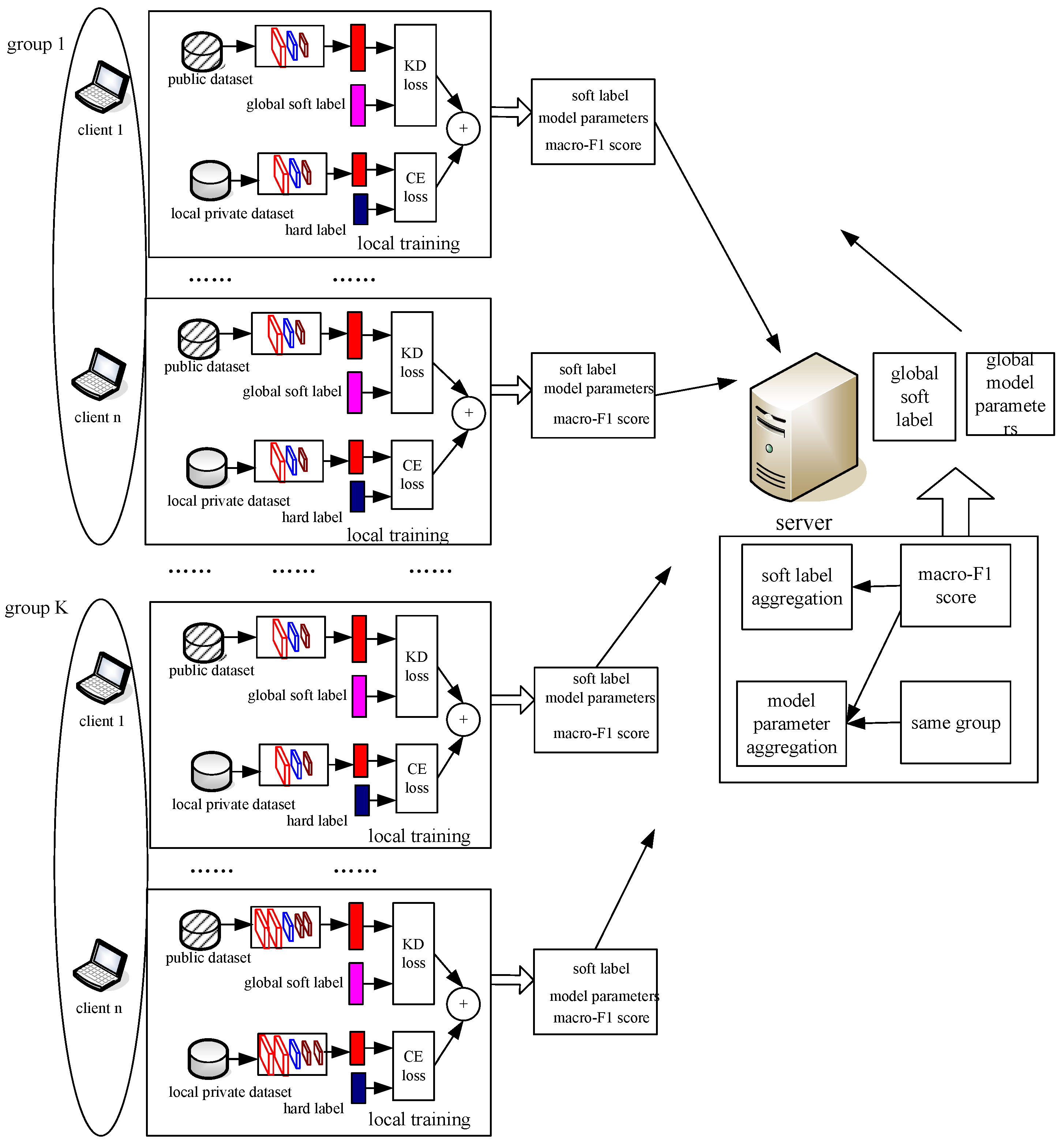
The proposed FL-based load identification system contains M clients. For the ith client, it has a local labeled dataset $D_i$ and shared unlabeled dataset $D_{pub}$. Since the load identification problem is typically formulated as an image classification problem, some image classification models such as VGG16, ResNet18, and ResNet34 are considered in the proposed system. The proposed algorithm consists of the following steps: First, clients with the same model are grouped to form k clusters, and then the FL process is performed. For all groups, each client utilizes the local dataset for local training, and the local load identification model is obtained. After that, the obtained model is used to generate the soft labels of the public dataset. The trained model parameters, soft labels, and macro-F1 score are uploaded to the server, where, based on the macro-F1 score, the global soft labels are obtained by parameter aggregation. The global load identification model with the same network architecture is also aggregated, after which the global soft labels and aggregated load identification model are downloaded to the clients. The block diagram of the proposed algorithm is shown in Figure 1.

3. Algorithm Description

3.1. Data Preprocessing

In this step, the Markov random fields (MTF) are utilized to convert the load data into $224\times 224$ RGB images.

A load measurement sequence $X=\{x_1,x_2,x_i,\dots ,x_n\}$ is first discretized into Q quantile bins (n is 224 and Q is 10 in this study). Each value in the sequence is then quantized using the quantiles $q_j$ ($j\in [1,Q]$), and each data point $x_i$ can be mapped to its corresponding quantile $q_i$. The Markov transition matrix W is written as

$$W=\left[\begin{array}{ccc}{w}_{11}& \dots & w_{1Q}\\ w_{21}& \dots & w_{2Q}\\ ⋮& \ddots & ⋮\\ w_{Q1}& \dots & w_{QQ}\end{array}\right]$$

(1)

where $w_{ij}=P(x_{t+1}\in q_j\mid x_t\in q_i)$.

In order to overcome the limitation where the transition probability can be obtained from multiple time intervals, a Markov Transition Field (MTF) is defined as

$$M=\left[\begin{array}{ccc}{m}_{11}& \dots & m_{1n}\\ m_{21}& \dots & m_{2n}\\ ⋮& \ddots & ⋮\\ m_{n1}& \dots & m_{nn}\end{array}\right]$$

(2)

where $m_{ij}=P(q_j\mid q_i)$ denotes the transition probability from quantiles $q_i$ to $q_j$.

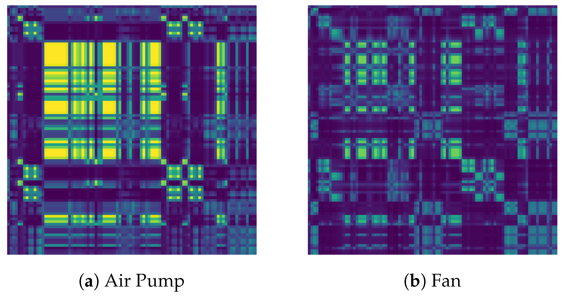
Finally, we map matrix M onto a two-dimensional image, where each element in the matrix corresponds to a pixel at the corresponding position in the image. Figure 2 describes the obtained images of the Air Pump and Fan data categories, respectively, where the former has a dark purple background, whereas the latter exhibits distinct and larger mixed regions of yellow and bright cyan. These two images differ in color distribution, so they can be used for image classification training.

3.2. Description of Algorithm at the Client

A model heterogeneity scenario is considered in this study where each client selects their local load identification model from three types of convolutional neural networks pretrained on ImageNet [11], namely ResNet18 [12], ResNet34, and VGG16 [13]. These networks exhibit distinct differences in terms of depth and parameter scale, and are suitable for the various computational and storage constraints of different clients.

To fully exploit the feature representation capability of pretrained models and minimize local training overhead, a fine-tuning strategy is used during local training at the client side that freezes the feature extraction parameters and trains only the classification parameters. Each load identification model and its local training process are described as follows.

The ResNet18 architecture is divided into two parts: a feature extraction module (one initial convolutional layer, four groups of residual blocks containing 16 convolutional layers in total, and one max-pooling layer) and a classifier module (one global average pooling layer and one final fully connected layer). During local training, the parameters of the entire feature extraction module including the weights of all convolutional and pooling layers are frozen to retain its capability for general image feature extraction. Only the final fully connected (FC) layer of the classifier module is designated as the target for learning. Its parameters are adjusted using local load data for classification requirements of load identification.

Similarly, the ResNet34 architecture consists of a feature extraction module (one initial convolutional layer, four groups of residual blocks containing 32 convolutional layers in total, and one max-pooling layer) and a classifier module (one global average pooling layer and one final FC layer). In local training, the parameters of the entire feature extraction module are also frozen, encompassing the weights of all convolutional and pooling layers, to preserve its general image feature extraction capacity. Only the final FC layer within the classifier module is chosen as the trained component. Its parameters are fine-tuned via local load data to meet the specific classification demands of load identification.

The VGG16 structure is divided into a feature extraction module (a stacked structure composed of 13 convolutional layers and 5 pooling layers) and a classifier module (3 fully connected layers). Throughout the local training process, the parameters of the entire feature extraction module remain frozen, keeping all convolutional and pooling layer weights in their pretrained state to maintain their image feature extraction capacity. Only the last FC layer of the classifier module is utilized for transfer learning training, where the parameters of this specific layer are updated using local load data to achieve classification.

Assume the labeled local private dataset is defined as $D_i=(x,y)$, where x denotes the input load image, $y\in 1,2,\dots ,C$ represents the load category label, and C is the total number of classes. The number of local data points is denoted as $n_i=\left|D_i\right|$. All clients share an unlabeled public dataset $D_{pub}=\left(x\right)$ with size $|D_{pub}|$. The model parameters of client i are denoted as ${\theta }_i$. For an input x, the model output logits vector is denoted as $z_i(x;{\theta }_i)\in {\mathbb{R}}^C$. Using a distillation temperature $T\ge 1$, the temperature-scaled softmax distribution can be expressed as $p_i^T(x;{\theta }_i)=\mathrm{softmax}(z_i(x;{\theta }_i)/T)$.

In the first round of local training, each client initializes its model parameters using the ImageNet pretrained model, and only the local private dataset is used for local training. Under this condition, the loss function of client i is defined as

$${\mathcal{L}}_{CE,i}^1\left({\theta }_i\right)={\displaystyle \frac{1}{n_i}}\sum _{(x,y)\in D_i}l(p_i(x;{\theta }_i),y)$$

(3)

where $l(·,·)$ denotes the cross-entropy loss, $p_i(x;{\theta }_i)=\mathrm{softmax}\left(z_i(x;{\theta }_i)\right)$, and $z_i(x;{\theta }_i)$ represents the model logits.

From the second round, besides the supervised cross-entropy loss based on the local private dataset, the loss function adds a distillation loss from the aggregated soft labels. This distillation loss employs the Kullback–Leibler (KL) divergence to quantify the discrepancy between the aggregated soft labels and the client’s temperature-scaled prediction distribution, which is written as [14]

$${\mathcal{L}}_{KD,i}^t\left({\theta }_i\right)={\displaystyle \frac{1}{|D_{pub}|}}\sum _{x\in D_{pub}}\mathrm{KL}\left(s_{agg}^{t-1}\left(x\right)\parallel p_i^T(x;{\theta }_i)\right)$$

(4)

where $s_{agg}^{t-1}\left(x\right)$ is the soft label aggregated from round $(t-1)$. The KL divergence is defined as

$$\mathrm{KL}(q\parallel p)=\sum _{c}q\left(c\right)\log {\displaystyle \frac{q\left(c\right)}{p\left(c\right)}}$$

(5)

Therefore, the total loss function for client i in round t ($t\ge 2$) is

$${\mathcal{L}}_i^t\left({\theta }_i\right)={\lambda }_{CE}{\mathcal{L}}_{CE,i}^t\left({\theta }_i\right)+{\lambda }_{KD}{\mathcal{L}}_{KD,i}^t\left({\theta }_i\right),t\ge 2$$

(6)

where ${\lambda }_{CE}$ and ${\lambda }_{KD}$ represent the weight parameters of the supervised cross-entropy loss and distillation loss, respectively, both of which are set to 0.5 in this study. Under this condition, supervised cross-entropy loss and distillation loss are equally important for model optimization. The equal weights balance their gradient contributions.

The client uses gradient descent to update the local trainable parameters:

$${\theta }_i^t={\theta }_i^{t-1}-\eta ,{\nabla }_{{\theta }_i}{\mathcal{L}}_i^{t-1}\left({\theta }_i^{t-1}\right)$$

(7)

where $\eta$ is the learning rate and ${\theta }_i^{t-1}$ denotes the model parameters in the $(t-1)$th round.

In the tth round, the ith client utilizes the model parameters ${\theta }_i^t$ for load identification of the public dataset $D_{pub}$. The generated soft labels by the ith client is given by

$$s_i^t\left(x\right)=\mathrm{softmax}(z_i(x;{\theta }_i^t)/T),\forall x\in D_{pub}$$

(8)

where $z_i^t\left(x\right)$ is the logits output for data x, and T is the distillation temperature.

Finally, the obtained soft labels $s_i^t\left(x\right)$ of the public dataset and the model parameters ${\theta }_i^t$ are unloaded to the server for aggregation.

3.3. Description of Algorithm at Server

In the tth communication round, the server aggregates the soft labels generated by each client on the public dataset $D_{pub}$ to obtain the global soft labels $s_{agg}^t\left(x\right)$. These global soft labels are subsequently downloaded to each client for local distillation training in the $(t+1)$th round. Moreover, for load identification models with the same structure, the server aggregates their model parameters to form the global model and also downloads them to the corresponding clients.

(a) Macro-F1-based soft label aggregation for public dataset

The aggregation weight for the ith client can be described as

$$w_i^t={\displaystyle \frac{{(F_i^t+\epsilon )}^{\gamma }}{{\sum }_{i=1}^M{(F_i^t+\epsilon )}^{\gamma }}}$$

(9)

where $F_i^t\in [0,1]$ denotes the macro-F1 score obtained by client i in the t-th round. $\gamma \in (0,1]$ denotes the smoothing index, and $\epsilon >0$ represents an infinitesimally small constant. $\gamma =0.5$ and $\epsilon ={10}^{-8}$.

After weighted averaging the soft labels, the aggregated soft labels of the public data in $D_{pub}$ are given by

$$s_{agg}^t\left(x\right)={\displaystyle \sum _{i=1}^M}{w}_i^t{s}_i^t\left(x\right),\forall x\in D_{pub}$$

(10)

Finally, the server downloads $s_{agg}^t\left(x\right)$ to each client for local distillation training in the $(t+1)$-th round.

(b) Trained model parameter aggregation for the same architecture

The server only performs parameter aggregation for load identification models with the same architecture, and then the aggregated parameters are downloaded to the corresponding clients.

Let $C_g$ denote the set of clients belonging to the same network architecture in the t-th round. The aggregated parameters ${\theta }_g^t$ are written as

$${\theta }_g^t=\sum _{i\in C_g}{w}_{i|g}^t{\theta }_i^t$$

(11)

$$\sum _{i\in C_g}{w}_{i|g}^t=1$$

(12)

where ${\theta }_i^t$ represents the model parameters uploaded by client i within the group, and $w_{i|g}^t$ is the normalized weight of the group.

Finally, the server downloads ${\theta }_g^t$ to the clients within $C_g$ for the next round of training.

4. Description of Experiment and Algorithm Performance

The experiments are carried out on hardware equipped with an NVIDIA GeForce RTX 4060 GPU, 32 GB of RAM, and an Intel Core i5-12600KF CPU. The models are constructed and trained using the PyTorch 2.0.0 deep learning framework within a Python 3.9.20 environment. Two publicly available datasets, WHITED and PLAID, are chosen for the experiment. The former contains high-frequency voltage and current recordings from household and small industrial appliances across multiple regions. Seven distinct load categories from this dataset are selected, namely, AirPump, Charge, Fan, FanHeater, Fridge, HairDryer, and LEDLight. The PLAID dataset collects 30 kHz voltage and current transient waveform data of household appliances from over 60 families in Pittsburgh. It has 11 appliance categories and more than 300 physical appliance units with over 1800 independent data records. The training data are evenly distributed among clients to maintain similar class distributions. The class distribution of training and test data for the WHITED and PLAID datasets are given in

Table 1. The class distribution of training and test data for the WHITED dataset.

	Client 1	Client 2	Client 3	Client 4	Client 5	Client 6	Test Data
Air Pump	211	211	211	211	211	215	423
Charge	400	400	400	400	400	400	800
Fan	158	158	158	158	158	158	316
Fan Heater	213	213	213	213	213	213	426
Fridge	241	241	241	241	241	245	483
Hair dryer	400	400	400	400	400	400	800
LED Light	400	400	400	400	400	400	800

and

Table 2. The class distribution of training and test data for the PLAID dataset.

	Client1	Client2	Client3	Client4	Client5	Client6	Test Data
Air_Conditioner	185	185	185	185	185	188	371
Compact_Fluorescent_Lamp	218	218	218	218	218	219	436
Fan	302	302	302	302	302	305	605
Fridge	78	78	78	78	78	78	156
Hairdryer	176	176	176	176	176	177	352
Heater	87	87	87	87	87	87	174
Incandescent_Light_Bulb	192	192	192	192	192	197	385
Laptop	267	267	267	267	267	270	535
Microwave	260	260	260	260	260	262	520
Vacuum	10	10	10	10	10	10	20
Washing_Machine	50	50	50	50	50	53	101

, respectively. The validation dataset is formed by randomly extracting 20% from the training dataset, and the public dataset has the same class distribution of clients. There are 4052 and 3665 public data points for the WHITED and PLAID datasets, respectively.

Among the six clients, Clients 1 and 4 employ the ResNet18 model, Clients 2 and 5 utilize the ResNet34 model, and Clients 3 and 6 adopt the VGG16 model. The batch size is uniformly set to 32. Each communication round encompasses local training across all clients, followed by the upload, aggregation, and subsequent distribution of soft labels. The Adam optimizer is chosen and can adaptively adjust the learning rate. The initial learning rate is 0.001, which is the general learning rate for fine-tuning the ImageNet pretrained network. The temperature parameter within the distillation loss is set to 2 as a compromise. For all experiments, there were 10 communication rounds of FL, and the random seed was set to 42, ensuring reproducibility of the experiments. Accuracy, Precision, Recall, and F1 score were calculated with macro averaging for performance analysis.

4.1. Description of Offline Training Performance

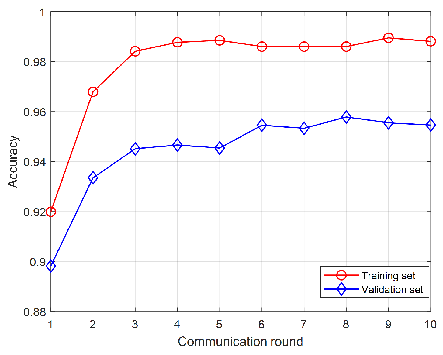
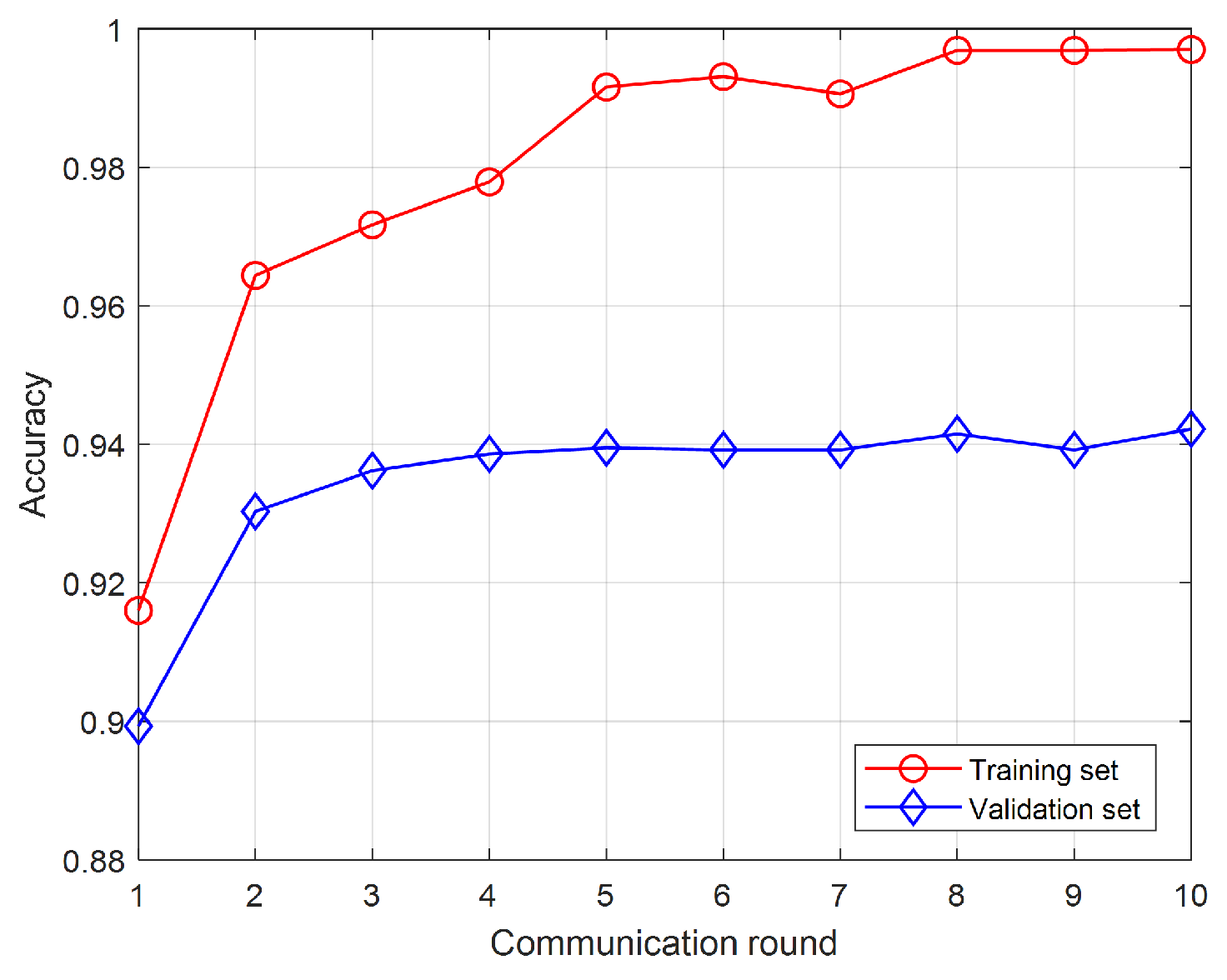
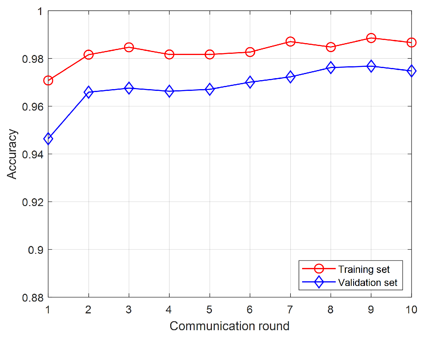
Figure 3, Figure 4 and Figure 5 describe the offline training performance of three different load identification models, showing that the accuracy of training and validation sets improved significantly after the first two rounds, before gradually stabilizing with good convergence performance. The validation accuracies are between 0.93 and 0.975. The VGG16-based load identification model has the best training performance among three models. According to the above experimental result, the proposed algorithm performs well in convergence and can be used for real conditions.

4.2. Load Identification Performance of the Proposed Algorithm

Table 3. Description of performance of different clients under WHITED dataset condition.

	Metric	Client 1 ResNet18	Client 2 ResNet34	Client 3 VGG16	Client 4 ResNet18	Client 5 ResNet34	Client 6 VGG16
Model
Accuracy		$0.9392\pm 0.0134$	$0.9236\pm 0.0083$	$0.9819\pm 0.0076$	$0.9340\pm 0.0098$	$0.9150\pm 0.0127$	$0.9817\pm 0.0107$
Precision		$0.9539\pm 0.0129$	$0.9393\pm 0.0130$	$0.9785\pm 0.0093$	$0.9482\pm 0.0115$	$0.9112\pm 0.0205$	$0.9819\pm 0.0149$
Recall		$0.9382\pm 0.0128$	$0.9234\pm 0.0071$	$0.9827\pm 0.0072$	$0.9320\pm 0.0098$	$0.9144\pm 0.0115$	$0.9817\pm 0.0099$
F1 Score		$0.9443\pm 0.0100$	$0.9297\pm 0.0075$	$0.9819\pm 0.0087$	$0.9376\pm 0.0081$	$0.9127\pm 0.0127$	$0.9818\pm 0.0136$

and

Table 4. Description of performance of different clients under PLAID dataset condition.

	Metric	Client 1 ResNet18	Client 2 ResNet34	Client 3 VGG16	Client 4 ResNet18	Client 5 ResNet34	Client 6 VGG16
Model
Accuracy		$0.6796\pm 0.0128$	$0.6183\pm 0.0087$	$0.6719\pm 0.0079$	$0.6993\pm 0.0101$	$0.6136\pm 0.0131$	$0.6705\pm 0.0104$
Precision		$0.6479\pm 0.0136$	$0.6209\pm 0.0125$	$0.7602\pm 0.0097$	$0.6489\pm 0.0118$	$0.5967\pm 0.0201$	$0.7941\pm 0.0152$
Recall		$0.6423\pm 0.0125$	$0.5229\pm 0.0074$	$0.5309\pm 0.0070$	$0.6756\pm 0.0095$	$0.5621\pm 0.0118$	$0.5090\pm 0.0102$
F1 Score		$0.6309\pm 0.0104$	$0.5272\pm 0.0078$	$0.5537\pm 0.0089$	$0.6544\pm 0.0084$	$0.5478\pm 0.0132$	$0.5148\pm 0.0133$

describe four machine learning metrics of the proposed algorithm under two dataset conditions, WHITED and PLAID. Under the former, all clients are found to perform well in load identification. For Clients 1 and 4 (ResNet18) and Clients 2 and 5 (ResNet34), all four evaluation metrics are approximately 0.94. VGG16 performs best in identification. However, under the latter condition, the performance worsens, which may be due to the following. From the class distribution shown in Table 2, the number of Vacuum, Washing Machine, Fridge, and Heater classes is very low, and the data imbalance problem may decrease the training performance. Second, under the PLAID dataset condition, the number of training data and public data points is lower than that under the WHITED dataset condition. Moreover, the load class to be classified is larger than that under the WHITED dataset condition. Less training data and more classes lead to worse classification.

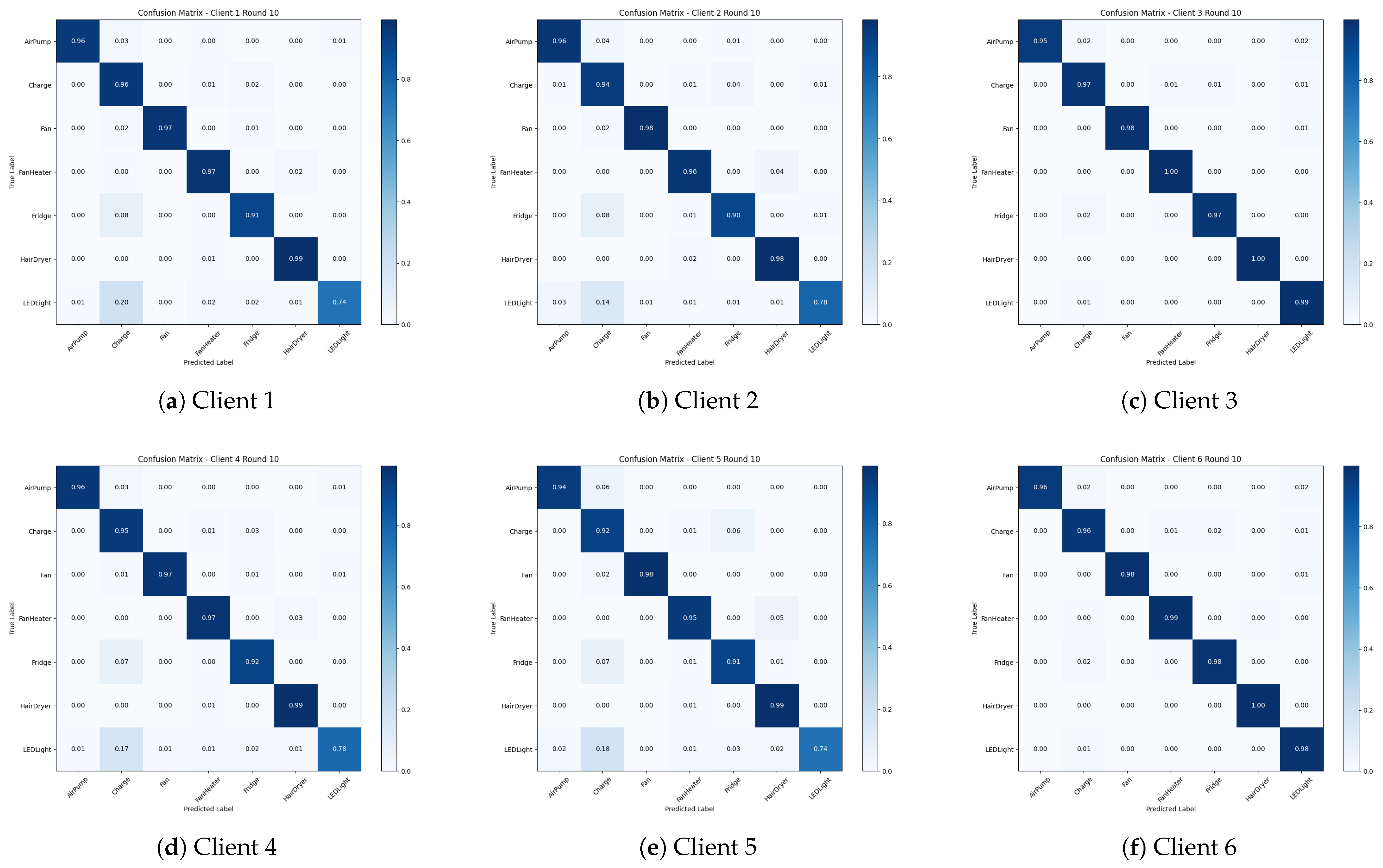
Taking the WHITED dataset as an example, Figure 6 describes the confusion matrix, showing that most load categories are correctly classified. For Clients 3 and 6 (VGG16), all four evaluation metrics reach approximately 0.97, and their confusion matrices similarly demonstrate a strong concentration of samples along the diagonal. These results indicate that the models achieve high classification accuracy and reliability, while maintaining excellent discriminative capability across different load categories. The VGG16 model achieves the best load identification performance among three load identification models. From the confusion matrix results, the LEDLight category performed significantly worse than the other categories on Clients 1, 2, 4, and 5. Some LEDLight were predicted as Charge, leading to prediction error, which may be because the VGG network is more suitable for the load images and it is easier to discover the features between small power loads.

In order to illustrate the communication efficiency of the proposed algorithm,

Table 5. Communication traffic of the proposed algorithm under the WHITED dataset condition.

	Communication Traffic
ResNet18	14.03 KB
ResNet34	14.03 KB
VGG16	112.03 KB
Soft label of each client	110.8 KB

describes the communication traffic of soft labels and model parameters under the WHITED dataset. Because the parameters of feature extraction are frozen, only a small number of parameters are uploaded to the server. Moreover, only the soft labels rather than the data are transmitted to the server. The communication traffic of soft labels is 110.8 KB. Thus, compared with the traditional centralized learning framework which requires all training data to be uploaded to the server, the proposed algorithm can reduce communication traffic. For computational analysis, the total running time of all clients is 3 h 48 min 38.15 s under the WHITED dataset condition. The time cost of aggregation at the server is 215.3 s. Compared with the large model application, the computational load of the proposed algorithm is acceptable. Note that more clients and communication rounds increased communication traffic and computation complexity. However, the identification performance will improve correspondingly. Thus, for practical application, there should be a trade-off between identification performance and algorithm complexity.

4.3. Algorithm Performance Comparison

In this section, performance metrics such as accuracy, precision, recall, and F1 score are averaged over all clients.

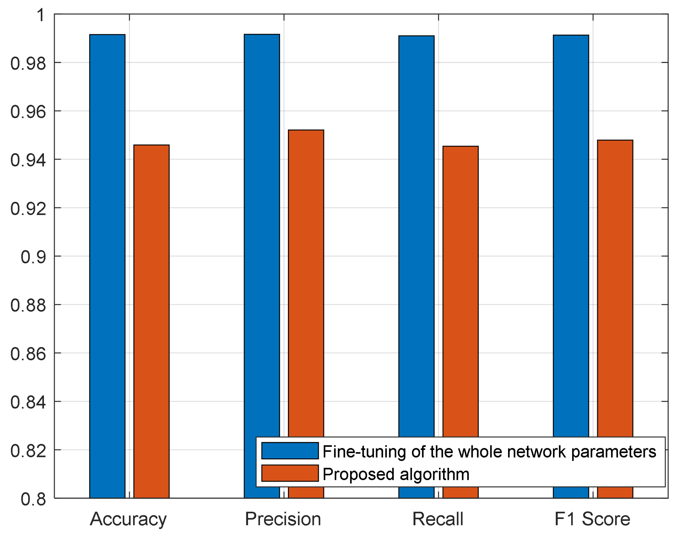
First, the fine-tuning of different model parameters under the WHITED dataset is compared with performance in Figure 7. From the experimental result, we can find that the four performance metrics from fine-tuning all network parameters can increase by about 4.5%, because all parameters of the identification model are trained.

Table 6. Comparison of communication traffic.

	Fine-Tuning of the Whole Network Parameters	Proposed Algorithm
ResNet18	42.65 MB	14.03 KB
ResNet34	81.21 MB	14.03 KB
VGG16	512.27 MB	112.03 KB

and

Table 7. Comparison of training time and aggregation time.

	Fine-Tuning of the Whole Network Parameters	Proposed Algorithm
training time	6 h 4 min 26.12 s	3 h 48 min 38.15 s
aggregation time	233.81 s	215.3 s

compare the communication traffic and running time. Since all parameters are trained, the training time taken to fine-tune all network parameters increased dramatically. Moreover, more model parameters should be uploaded to the server. Although the performance of the proposed algorithm is worse than that of the compared method, communication traffic and running time are much lower, so it is more suitable for practical applications.

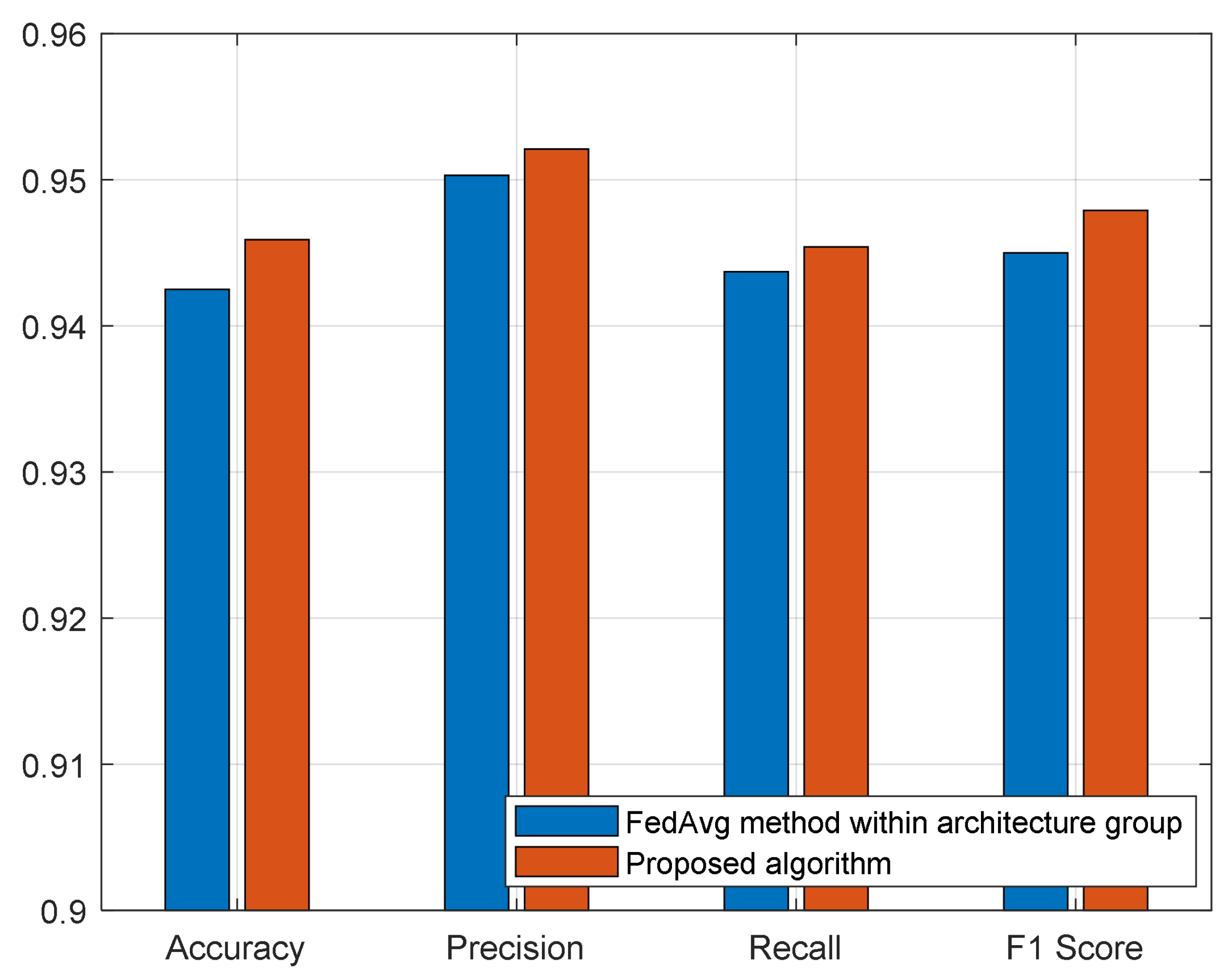
Second, Figure 8 compares the performance with the FedAvg method with the architecture group under the WHITED dataset. It can be seen that the load identification of the proposed algorithm performs better than that of FedAvg with the architecture group, attributed to the additional soft label aggregation. Moreover, to compare communication traffic, except for trained model parameters, the proposed algorithm should unload the soft labels to the server, which is only 110.8 KB in size. For computational complex analysis, the total training time of the FedAvg method with the architecture group is 3 h 47 min 17.88 s. Because only distillation loss is added to the loss function, the proposed algorithm has a similar computational complexity to the FedAvg method with the architecture group.

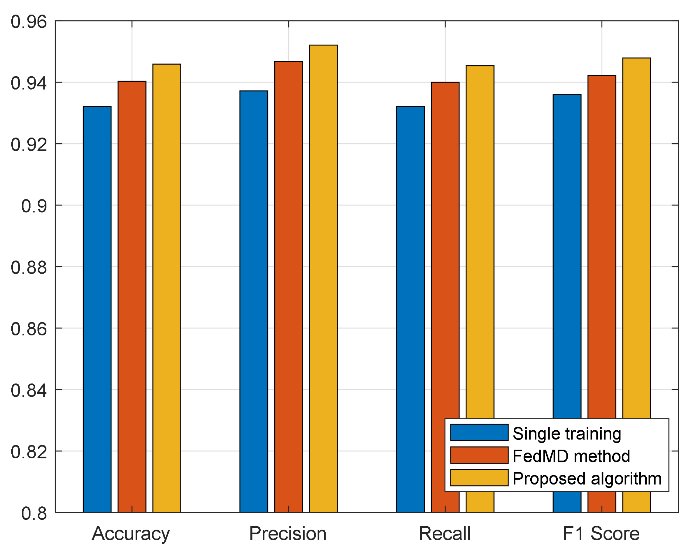
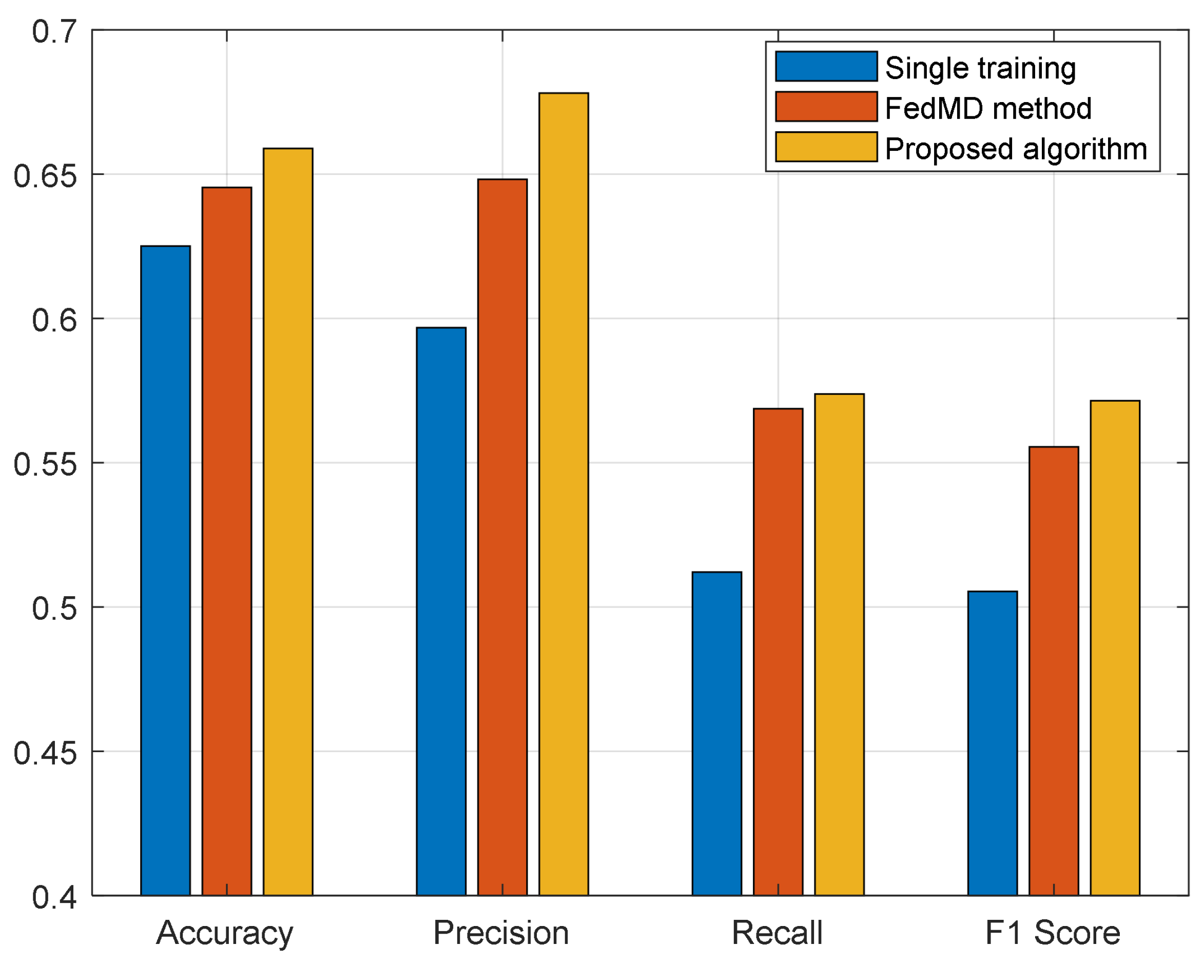
Third, different training methods, specifically single training and the FedMD method, are chosen to compare performance under the WHITED and PLAID dataset conditions, as shown in Figure 9 and Figure 10. The experimental results show that the proposed algorithm performs best in load identification among three methods. Under the former dataset condition, the four machine learning metrics of the proposed algorithm can increase by about 1% for single training and 0.5% for the FedMD method. Under the latter condition, taking accuracy as an example, the improvement in the proposed algorithm is 3.3% for single training and 1.3% for the FedMD method. Thus, through model parameter aggregation of the same model structure and federated distillation with the public dataset, both the classification performance and the generalization capability of the client model can be effectively enhanced.

Finally, we adopt Welch’s t-test to verify whether the difference in performance between two compared methods is statistically significant, which is taken as p < 0.05 in the experiment. Taking the average F1 score as an example, we perform three independent experimental runs.

Table 8. The results of Welch’s t-test for different conditions.

	p Value
Fine-tuning of different model parameters and the proposed algorithm (WHITED dataset)	0.000006
FedAvg method with architecture group and the proposed algorithm (WHITED dataset)	0.000325
FedMD method and the proposed algorithm (WHITED dataset)	0.006968
Single training and the proposed algorithm (WHITED dataset)	0.000461
FedMD method and the proposed algorithm (PLAID dataset)	0.000326
Single training and the proposed algorithm (PLAID dataset)	0.000024

describes the p value of different conditions, where the result shows a statistically significant difference between the compared and proposed algorithms.

5. Conclusions

In this article, an FL- and KD-based load identification algorithm under a heterogeneous model condition is proposed. It effectively combines the privacy-preserving advantages of federated learning and the flexibility of knowledge distillation for collaborative learning among client models with different architectures. The experimental results demonstrate that the proposed algorithm can significantly improve identification performance. Future research will formally investigate the interplay between global soft-label distillation and group-wise parameter aggregation. Moreover, since macro-F1 measured on clients’ own local private data may generate inflated scores, we will focus more on explicitly discussing this risk.

Nevertheless, the proposed method has certain limitations. The load identification accuracy differs in various public datasets. We will develop effective data preprocessing techniques to reduce this dataset-induced fluctuation in performance. Furthermore, the growing scale and diversity of clients lead to large time gaps in parameter arrival at the server. Asynchronous federated learning will be adopted to tackle the asynchronous transmission of model parameters.

References

1. Mitra, A.; Ghosh, S.; Mohapatra, A.; Chakrabarti, S. Data-Driven Sparsification and Multi-Resolution Analysis-Based Framework for Load Identification. IEEE Trans. Smart Grid 2024, 15, 2387–2390. [Google Scholar] [CrossRef] [Scilit]
2. Yuan, J.; Jin, R.; Wang, L.; Wang, T. A Nonintrusive Load Identification Method Based on Dual-Branch Attention GRU Fusion Network. IEEE Trans. Instrum. Meas. 2024, 73, 2521710. [Google Scholar] [CrossRef] [Scilit]
3. Asad, M. Feature-Centric Approaches to Non-Intrusive Load Monitoring and Appliance Identification. Master’s Thesis, Concordia University, Montréal, QC, Canada, 2025. [Google Scholar]
4. Asres, M.W.; Girmay, A.A.; Camarda, C.; Tesfamariama, G.T. Non-intrusive load composition estimation from aggregate ZIP load models using machine learning. Electr. Power Energy Syst. 2019, 105, 191–200. [Google Scholar] [CrossRef] [Scilit]
5. Pei, J.; Liu, W.; Li, J.; Wang, L.; Liu, C. A Review of Federated Learning Methods in Heterogeneous Scenarios. IEEE Trans. Consum. Electron. 2024, 70, 5983–5999. [Google Scholar] [CrossRef] [Scilit]
6. McMahan, H.B.; Moore, E.; Ramage, D.; Hampson, S.; Arcas, B.A. Communication-Efficient Learning of Deep Networks from Decentralized Data. In Proceedings of the 20th International Conference on Artificial Intelligence and Statistics; ML Research Press: Cambridge, MA, USA, 2016. [Google Scholar]
7. Kim, J.; Park, S.; Kwak, N. Paraphrasing Complex Network: Network Compression via Factor Transfer. arXiv 2018, arXiv:1802.04977. [Google Scholar]
8. Smith, V.; Chiang, C.; Sanjabi, M.; Talwalkar, A. Federated Multi-Task Learning. In Proceedings of the 31st International Conference on Neural Information Processing Systems; ACM: New York, NY, USA, 2017. [Google Scholar]
9. Wang, H.; Si, C.; Zhao, J. A Federated Learning Framework for Non-Intrusive Load Monitoring. arXiv 2025, arXiv:2104.01618. [Google Scholar]
10. Pan, Z.; Wang, H.; Li, C.; Wang, H.; Zhao, J. PerFedNILM: A Practical Personalized Federated Learning-based Non-Intrusive Load Monitoring. Ind. Artif. Intell. 2024, 18, 78–92. [Google Scholar] [CrossRef] [Scilit]
11. Deng, J.; Dong, W.; Socher, R.; Li, L.-J.; Li, K.; Fei-Fei, L. ImageNet: A large-scale hierarchical image database. In Proceedings of the 2009 IEEE Conference on Computer Vision and Pattern Recognition, Miami, FL, USA; IEEE: Piscataway, NJ, USA, 2009; pp. 248–255. [Google Scholar]
12. He, K.; Zhang, X.; Ren, S.; Sun, J. Deep Residual Learning for Image Recognition. In Proceedings of the 2016 IEEE Conference on Computer Vision and Pattern Recognition (CVPR), Las Vegas, NV, USA; IEEE: Piscataway, NJ, USA, 2016; pp. 770–778. [Google Scholar]
13. Reddy, V.K.; Reddy, S.P.; Naidu, K.; Sekhar, P.N. Maximizing Efficiency in Face Recognition:A VGG16and Max Pooling Approach. Grenze Int. J. Eng. 2023, 9, 176. [Google Scholar]
14. Guo, S.; Chen, H.; Liu, Y.; Yang, C.; Li, Z.; Jin, H.C. Heterogeneous Federated Learning Framework for IIoT Based on Selective Knowledge Distillation. IEEE Trans. Ind. Inform. 2025, 21, 1078–1089. [Google Scholar] [CrossRef] [Scilit]
Figure 1. Block diagram of the proposed algorithm.
Applsci 16 08533 g001
Figure 2. MTF-based load images.
Applsci 16 08533 g002
Figure 3. Training performance of ResNet 18 (Client 1).
Applsci 16 08533 g003
Figure 4. Training performance of ResNet 34 (Client 2).
Applsci 16 08533 g004
Figure 5. Training performance of VGG16 (Client 3).
Applsci 16 08533 g005
Figure 6. Confusion matrix for different clients under WHITED dataset.
Applsci 16 08533 g006
Figure 7. Comparison of performance of fine-tuning of different model parameters under WHITED dataset.
Applsci 16 08533 g007
Figure 8. Comparison of performance of FedAvg method with the architecture group under WHITED dataset.
Applsci 16 08533 g008
Figure 9. Comparison of performance with different training methods under WHITED dataset.
Applsci 16 08533 g009
Figure 10. Comparison of performance with different training methods under PLAID dataset.
Applsci 16 08533 g010