Short-Term Electricity Consumption Forecasting for a University Campus: A Hybrid SWT–Frequency Attention–TCN Approach

Featured Application

This study presents an applicable decision-support approach for short-term electricity consumption forecasting. The proposed method can be used in building, campus, and energy management systems for load planning, demand side management, reducing energy costs, identifying peak loads in advance, and integrating renewable energy sources into the system more effectively. By utilizing historical electricity consumption together with hour and day-of-week calendar variables, the developed forecasting model can support energy managers in real-time operational and resource planning decisions.

Abstract

This study proposes a hybrid deep learning model based on the Stationary Wavelet Transform (SWT), a Frequency Attention mechanism, and a Temporal Convolutional Network architecture (TCN) for short-term electricity consumption forecasting at the university campus scale. The study utilizes a total of 40,896 observations collected from the central campus of Afyon Kocatepe University between 1 March 2024 and 30 April 2025, at 15 min intervals. Feature ablation analysis was conducted to determine the contribution of the candidate input variables. The results show that the inclusion of meteorological variables did not provide any additional improvement in forecasting accuracy. Therefore, the final compact model uses only historical electricity consumption together with the Hour and Day of Week calendar variables, which are known at the forecast origin. In the proposed model, the historical electricity consumption sequence is first decomposed into different frequency components using SWT, and the more informative frequency scales are adaptively weighted through the Frequency Attention mechanism. The resulting multiscale representation is then processed by the TCN architecture to model temporal dependencies and directly predict electricity consumption one hour ahead. Model performance was evaluated using the MAE, MSE, RMSE, MAPE, SMAPE, and R² metrics under rolling and anchored walk-forward validation strategies. The proposed SWT + Frequency Attention + TCN model achieved the best overall performance among the evaluated models, with an RMSE of 10.614 and an R² of 0.942 under the rolling walk-forward strategy and an RMSE of 10.286 and an R² of 0.946 under the anchored walk-forward strategy. The findings demonstrate that the integration of SWT-based multiscale representation, selective frequency weighting, and TCN-based temporal dependency modeling provides an effective and robust framework for short-term campus electricity consumption forecasting.

1. Introduction

Population growth, industrialization, and technological advancement are among the primary drivers of the continuing increase in electricity consumption [1]. According to Enerdata’s 2025 report, global energy consumption increased by 2.2% in 2024, surpassing the average annual growth rate recorded during the 2010–2019 period [2]. This rapid growth in energy demand has made the accurate and reliable management of the supply–demand balance increasingly critical. In this context, the building sector is particularly important because it accounts for a substantial proportion of total electricity consumption. Residential buildings, in particular, represent one of the largest electricity-consuming segments of the global building stock [3]. University campuses also constitute major electricity consumers because they comprise facilities with diverse operational and occupancy profiles, including educational buildings, laboratories, administrative units, libraries, cafeterias, social facilities, and support service areas. Electricity consumption on university campuses exhibits highly dynamic patterns depending on the academic calendar, occupancy levels, operating schedules, and meteorological conditions [4]. Managing these dynamic consumption patterns requires robust and reliable forecasting models. Accurate forecasting of campus electricity consumption can provide significant benefits, including improved energy management, reduced operating costs, more effective resource planning, and better maintenance of the supply–demand balance. Previous research on campus microgrids has demonstrated that effective energy management can reduce operating costs, increase the utilization of renewable energy resources, and improve the operational efficiency of energy storage systems [5]. Moreover, university campuses are complex energy systems comprising heterogeneous load profiles. Their variable and interconnected load characteristics therefore create a distinctive challenge for energy management and electricity demand forecasting [6].

Considering these challenges, the development of accurate electricity consumption forecasting models has become essential. Numerous forecasting approaches have been investigated over the years. Early studies in this field primarily relied on statistical forecasting methods. These methods offer several advantages, including relatively simple mathematical structures, high interpretability, and low computational requirements. However, they also have important limitations because they generally rely on assumptions of stationarity, linearity, and predefined probability distributions. Consequently, such models may be insufficient to capture complex, nonlinear, and time-varying electricity consumption patterns [7,8]. Electricity consumption is influenced by numerous external factors, including temperature, geographic location, industrial activity, population density, occupancy patterns, operating hours, weekday–weekend variations, and special periods. Therefore, the forecasting performance of conventional statistical models may deteriorate under sudden load variations, irregular consumption patterns, and complex multivariate dynamics [9,10]. In a study combining statistical models with machine learning methods, Grandón et al. [11] showed that regression models have poor performance when used alone. The same study demonstrated that integrating regression models with machine learning techniques improved their forecasting performance. Sahin et al. [12] compared linear and nonlinear forecasting approaches. In this context, ANN and Multiple Linear Regression (MLR) methods were used. The results showed that the ANN model was more successful. The main reason for this is that ANN can model nonlinear relationships more effectively. Therefore, ANN performed better than MLR in energy efficiency prediction. Unlike statistical models, machine learning models focus on learning nonlinear relationships, complex patterns, and multivariate structures in data. Commonly used machine learning models in electricity energy forecasting include artificial neural networks [13], support vector machines [14], decision trees [15], random forest [16], and extreme gradient boosting (XGBoost) [17]. In one study, Kusumoto et al. [18] aimed to predict the municipal-scale electricity demand in Japan. A multilayer perceptron (MLP)-based machine learning model was used in the study. Ultimately, the model captured local consumption characteristics better than the classical proportional distribution method and achieved high accuracy in most regions. In a study contributing to machine learning prediction models, Tercha et al. [19] used the augmented decision tree regression (ADTR) method for solar radiation estimation. The ADTR model was compared with the LR and NNR methods and yielded more successful results with lower error values. In the study, the R² value of ADTR was calculated as 0.901. Deep learning models are more successful than machine learning models in learning long-term dependencies, sequential patterns, and nonlinear relationships. Models such as long short-term memory (LSTM) [20], gated recurrent unit (GRU) [21], and convolutional neural networks (CNN) [22] successfully represent sudden changes in energy and temporal dynamics by analyzing past consumption behaviors. El-Azab et al. [23] compared the performance of machine learning and deep learning models for hourly electricity demand forecasting. ANN, LSTM, GRU and ANFIS methods were used in the forecasts. For working days, the highest accuracy was achieved with ANFIS in winter at 99.9%. Hybrid models are methods developed to improve forecasting success by combining the best aspects of different models. Various models have been developed in the literature, such as statistical-machine learning [24], machine learning–deep learning [25] or deep learning optimization algorithms. In a study contributing to the literature, Ullah et al. [26] proposed an attention mechanism hybrid CNN-BiGRU model for short-term electric load estimation. The CNN-BiGRU–Attention model was compared with different deep learning models based on CNN-LSTM, DNN and CNN-BiLSTM. MAPE was calculated as 0.51% for the proposed model. In another study, Chen et al. [27] proposed a hybrid deep learning model for building electrical load estimation. In the model, load components were separated using CEEMDAN, FFT, and K-means, followed by an MKDCN-LSTM structure and GWO-based weight optimization. According to the results, the proposed method showed better prediction performance than CNN, LSTM, CNN-LSTM, BiLSTM, TCN, ARIMA, XGBoost, and FBProphet-LSTM models.

In literature reviews, researchers have examined the advantages, performance, and differences in traditional deep learning models, such as single-structure models like CNN and LSTM, or hybrid models like CNN-LSTM. This study utilizes electricity consumption data collected from Afyon Kocatepe University to perform short-term load forecasting. To this end, a hybrid multi-scale deep learning framework integrating the Stationary Wavelet Transform (SWT), a frequency attention mechanism, and a Temporal Convolutional Network (TCN) is proposed. The model decomposes the historical electricity consumption signal into multi-resolution frequency components, while calendar variables are incorporated separately. The most informative frequency components of the decomposed signals are then weighed through an attention mechanism, enabling the model to learn interactions among the input variables. Finally, the temporal dependencies are modeled using the TCN architecture to forecast future electricity consumption. The primary objective of this study is to improve the accuracy and reliability of short-term electricity consumption forecasting. Within this framework, low-frequency long-term trends and high-frequency abrupt variations in electricity consumption series are considered simultaneously. The study initially considers meteorological variables as candidate predictors; however, feature-ablation analysis is used to determine whether their inclusion provides additional forecasting benefit. The final compact model relies on historical electricity consumption and forecast-origin calendar information. In this way, the study aims to obtain more accurate, reliable, and interpretable forecasting results. The methodological rationale of this study does not rely on the sequential combination of SWT, Frequency Attention, and TCN itself, but on the controlled integration of these components within a leakage-safe forecasting framework. SWT decomposes the historical electricity consumption sequence into low- and high-frequency components while preserving their temporal alignment. The Frequency Attention mechanism then adaptively weights the SWT-derived components rather than assuming that all frequency bands contribute equally to forecasting. Subsequently, the TCN models temporal dependencies within the weighted multiscale representation through causal and dilated convolutions. Thus, the proposed framework combines multiscale representation, selective frequency weighting, and temporal dependency modeling within a unified forecasting pipeline, while its effectiveness is further examined through controlled ablation and extensive benchmark comparisons. The contribution of this study does not lie in the use of established components such as SWT or TCN individually. Rather, the methodological contribution lies in the selective reweighting of a multiscale electricity consumption representation through a lightweight frequency-scale attention mechanism, the isolation of the contribution of each component through controlled ablation experiments, and the systematic evaluation of the resulting framework under a leakage-safe temporal evaluation protocol. The main contributions of this study to the literature are summarized below:

• Fifteen-minute electricity consumption data from a university campus was evaluated, and an application area was presented for short-term prediction of complex consumption behaviors at the campus scale.
• A multi-scale electricity consumption representation based on the Stationary Wavelet Transform (SWT) is employed to separate the historical consumption sequence into different frequency components.
• Rather than uniformly incorporating the frequency components obtained through SWT into the forecasting process, a selective feature representation is introduced in which the frequency scales that are more informative for prediction are adaptively weighted through the Frequency Attention mechanism.
• The TCN architecture was used to model both short-term and long-term temporal dependencies together.
• To more accurately represent real-world forecasting conditions, rolling and anchored walk-forward validation strategies were evaluated together. The contribution of each component of the proposed architecture to prediction performance has been demonstrated through comprehensive ablation analyses.

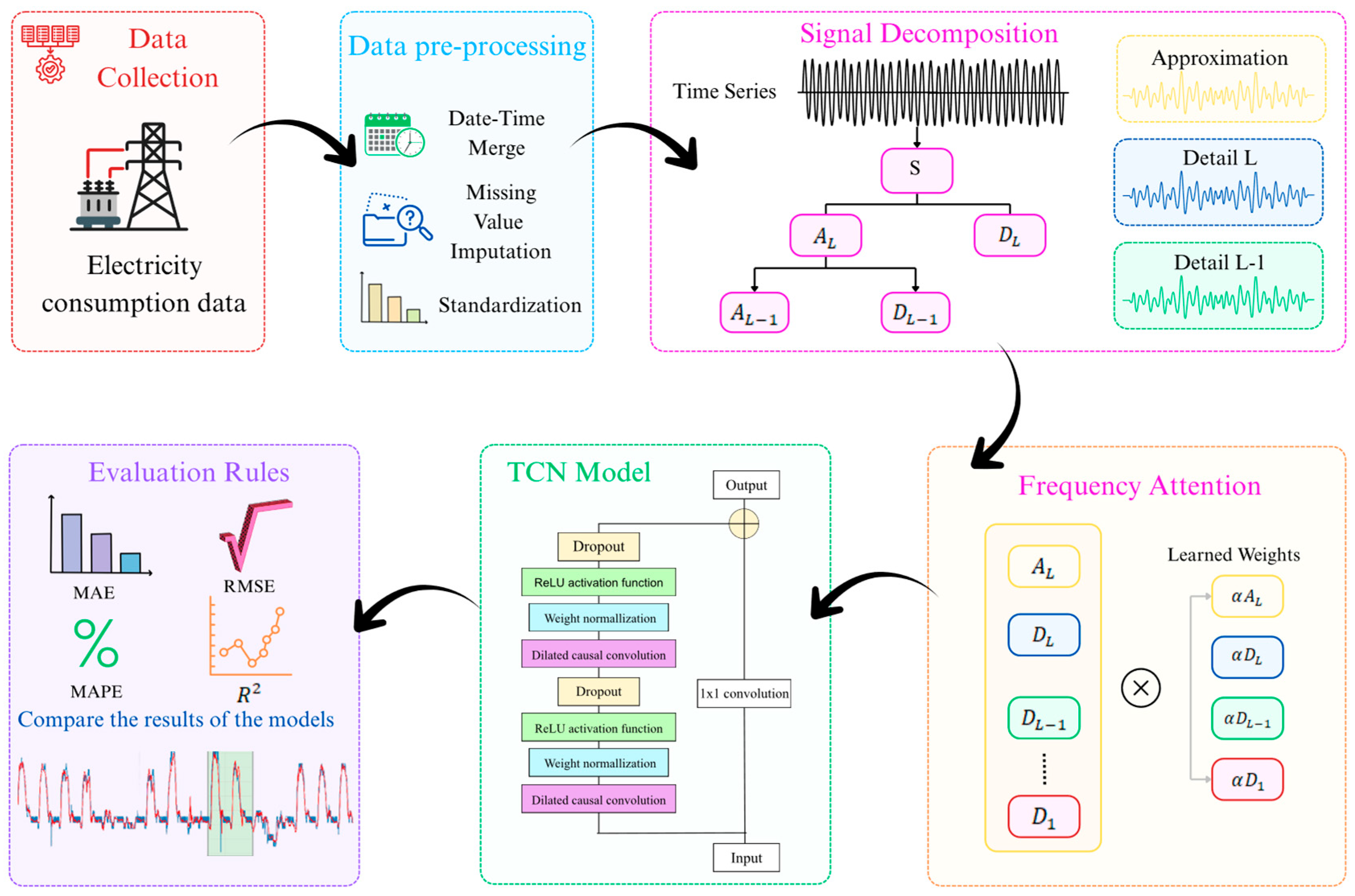
The remainder of this paper is organized as follows. Section 2 describes the dataset used in this study, the proposed hybrid model for electricity consumption forecasting, and the performance evaluation metrics. Section 3 presents the results obtained from the evaluated models, while Section 4 discusses the findings. The overall schematic representation of the study is presented in Figure 1.

2. Materials and Methods

This section presents the dataset used in the study, the data preprocessing steps, the SWT-based data parsing technique, the walk-forward validation technique, and details of the proposed model.

2.1. About the Data Set

The data used in this study were obtained from the central campus of Afyon Kocatepe University. Afyon Kocatepe University, where the study was conducted, is located in Afyonkarahisar province, in the Inner Western Anatolia region of Turkey’s Aegean Region. Afyonkarahisar, in terms of climate characteristics, exhibits a continental-steppe character that is more similar to the climate of Central Anatolia. Winters in the province are generally cold and snowy, while summers are hot and dry. The average annual temperature in Afyonkarahisar is approximately 11.3 °C. The average sunshine duration is approximately 6.7 h per day, and the total annual rainfall is approximately 443 mm. The average relative humidity in the region is given as approximately 64.87%, and the average pressure is approximately 897.7 hPa. 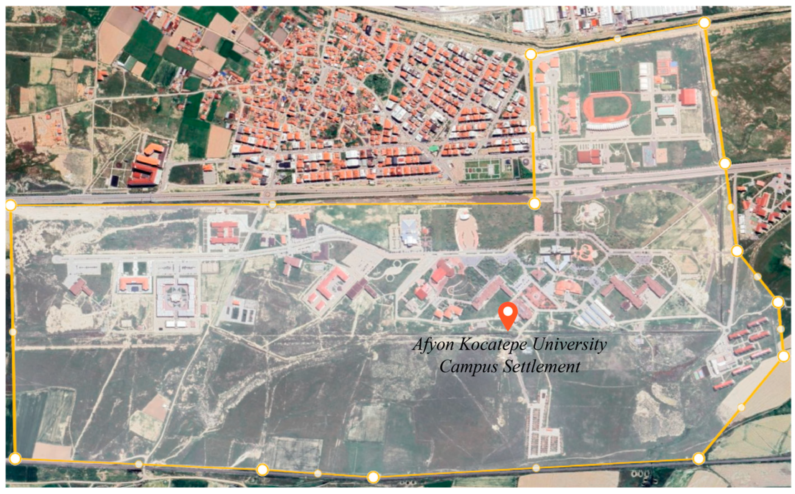The total annual solar radiation of Afyonkarahisar is approximately in the range of 1550–1650 kWh/m²-year [7]. These climatic characteristics are influential factors in evaluating the campus electricity consumption profile. As of 2026, the number of active students at Afyon Kocatepe University is 30.340. The university has 1111 academic staff members, and when administrative, worker, and contract employees are considered together, the number of non-academic staff is 961. The university comprises 13 faculties, 3 graduate schools, 3 schools, 1 state conservatory, and 14 vocational schools. The Ahmet Necdet Sezer Campus, which is the focus of this study, includes numerous units with different usage profiles such as faculties, institutes, colleges, conservatories, vocational schools, cafeterias, social facilities, research centers, laboratories, libraries, and sports areas. In this study, 30 main buildings with active energy consumption on the central campus were taken into consideration. A bird’s-eye view of the campus under investigation is shown in Figure 2.

The dataset used in this study consists of electricity consumption and meteorological measurement data. Meteorological data were collected using a Davis Instruments Vantage Pro2 weather station (Davis Instruments Corporation, Hayward, CA, USA) equipped with a solar radiation sensor. In the raw dataset, solar radiation intensity was recorded in W/m². The data covers an approximately 14-month period between 1 March 2024 and 30 April 2025. Measurements were recorded at 15 min intervals, and the dataset contains a total of 40.896 observations. During the measurement period, the mean temperature, relative humidity, wind speed, atmospheric pressure, and solar irradiance were calculated as 12.74 °C, 63.27%, 1.77 m/s, 761.87 hPa, and 200.04 W/m², respectively. Over the same period, the mean electricity consumption per 15 min interval was 126.13 kWh. Detailed statistical information on the dataset and the number of missing values are presented in

Table 1. Basic descriptive statistics for the dataset.

Variable	Unit	Mean Value	SD	Min	Q1	Median	Q3	Max	Missing Number
Temperature	°C	12.74	9.33	−11.30	5.30	11.90	19.40	37.80	2
Humidity	%	63.27	24.73	0	44.00	68.00	85.00	100.00	2
Wind speed	m/s	1.77	1.77	0.00	0.40	1.30	2.70	15.20	2
Pressure	hPa	761.87	5.71	748.80	757.50	761.10	765.90	777.70	2
Solar irradiance	W/m2	200.04	290.50	0.00	0.00	5.00	351.00	1155.00	2
Electricity consumption	kWh/15 min	126.13	43.97	31.05	103.50	113.85	134.55	341.55	2

.

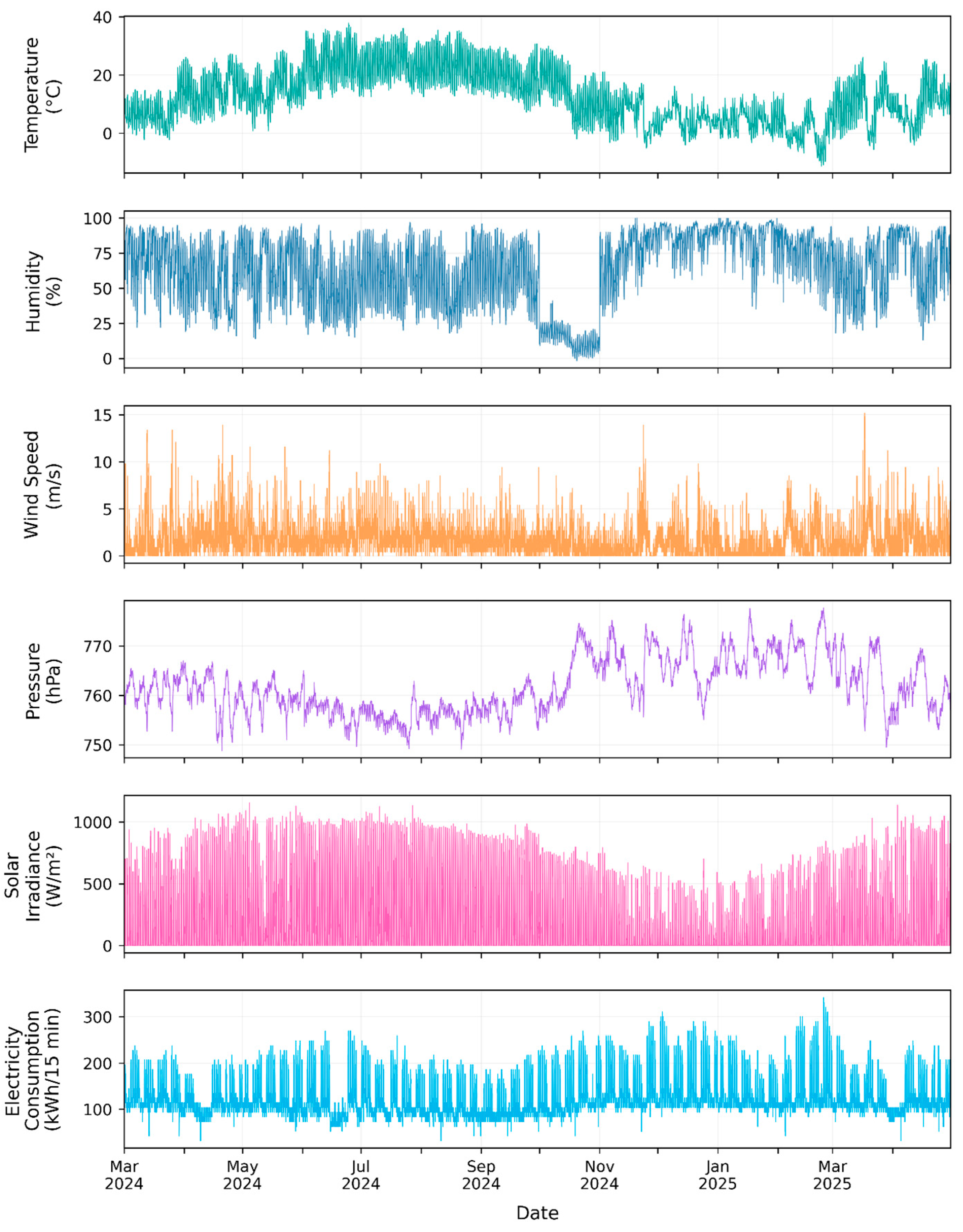
Figure 3 presents time series graphs of electricity consumption and meteorological variables used in the study. These graphs show the temporal changes, seasonal trends, and short-term fluctuations of the variables within the observation period.

Meteorological variables were available in the original dataset and were initially considered as candidate predictors. However, the feature ablation analysis showed that their inclusion did not improve forecasting performance. Therefore, they were excluded from the final compact forecasting model.

2.2. Data Preprocessing

Data preprocessing is a crucial step in improving the performance of predictive models. Preprocessed data provides cleaner inputs to the model, making it easier to use. This contributes to improving the predictive accuracy of the models. One of the common problems in time series analysis is missing data. Missing data leads to distortion of the temporal structure, erroneous processing of historical information, and a decrease in the reliability of model results. Some of the data used in the study could not be measured due to sensor errors or external factors. Upon examination, 12 humidity values were found to be negative, and these values were set to the minimum value of 0%. All data, except for solar radiation data, were filled in using averages. Missing data on solar radiation are not suitable for filling in the average due to night hours. Therefore, the linear interpolation method was used for this data [7]. The mathematical expression for the linear interpolation method is given in Equation (1).

$$y=y_1+\left({\displaystyle \frac{\left(x-x_1\right)(y_2-y_1)}{x_2-x_1}}\right)$$

(1)

In Equation (1), $x_1$ e represents the time point before the missing data, and $x_2$ represents the time point after the missing data. $y_1,$ is the known consumption value at time $x_1{.y}_2,$ is the known consumption value at time $x_2.$ $x$, is the time when the missing data is located, and $y$ is the estimated value obtained by interpolation [7]. After completing the missing data, the raw data was converted to time series format. The date and time columns within the dataset were combined to create a single time value. This preserved the chronological structure necessary for electricity consumption forecasting. Furthermore, the hour and day of the week features were converted from this single time value into a time series and provided as additional input to the model.

In order to avoid disrupting the time series structure, prevent data leakage and represent real-world prediction scenarios more accurately, the walk-forward validation approach has been used [28]. In this context, two different validation structures, rolling walk-forward and anchored walk-forward, have been examined. In the walk-forward validation procedure, the outer training and test periods were first defined chronologically. In the first fold of the rolling strategy, the outer training window covers 60% of the total dataset, while the subsequent test window covers 10%. The last 15% of each outer training period was allocated chronologically as the validation set, while the preceding 85% was used as the train core set. Therefore, in the first fold, the train core set corresponds to approximately 51% of the total dataset, the validation set to approximately 9%, and the test set to 10%. Although the outer training window expands in the subsequent folds of the anchored strategy, the rule of allocating the last 15% of the current training period as the validation set was maintained for every fold. The data points were not randomly shuffled at any stage.

The train core set was used to learn the model parameters, whereas the validation set was not included in gradient-based weight updates and was used only for monitoring validation loss, learning rate scheduling, and early stopping. Feature and target standardization parameters were calculated exclusively from the train core set and were applied to the validation and test sets without refitting. Data from the test period were not used at any stage of model development or selection and were evaluated only for the calculation of final performance on unseen data.

In this study, approximately 60% of the total data defines the outer training window in the first fold, while the subsequent 10% forms the test window. Accordingly, the outer training interval consists of 24.537 samples. This value corresponds to approximately 256 days. The test window consists of 4090 samples and represents a time interval of approximately 43 days. In the next fold, the time interval was shifted forward by approximately 10% of the total data. Within each walk-forward strategy, the test periods of consecutive folds do not overlap. After the test period of one fold ends, the test period of the next fold begins at the following 15 min time point. Therefore, the same target time point is not predicted in more than one test fold within the same walk-forward strategy. In the rolling and anchored strategies, the corresponding folds were intentionally evaluated over the same test periods. This enabled the performance of the two different training window approaches to be directly compared on the same unseen observations. Rolling and anchored predictions were evaluated separately, and no merging or averaging of predictions was performed across the two strategies. Performance metrics were first calculated separately for each test fold, and the mean and standard deviation of the fold-level results were then reported for each strategy.

In the rolling walk-forward approach, the training window is kept at a fixed length and shifted forward along the time axis. At each fold, the model is retrained using the most recent historical observations. Then the model is evaluated on the next unseen test period. This structure allows for a more realistic measurement of out-of-sample prediction performance [29]. In the anchored walk-forward approach, the training window is maintained from the initial date and expands at each fold. 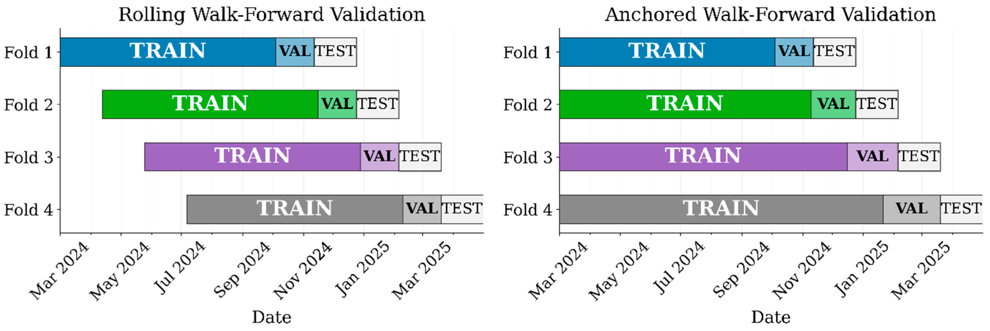Thus, the model continues to learn by using all the information from the past [30]. An example of rolling walk-forward and anchored walk-forward training and testing methodology for the dataset is given in Figure 4.

In the rolling walk-forward method, the training window maintains a fixed size of approximately 256 days, but the window is shifted forward with each fold. This allows the model to adapt to changing consumption behaviors over time. In the anchored walk-forward method, the training set grows with each fold. Therefore, the model can learn not only current behaviors but also long-term consumption patterns and seasonal variations. The time intervals for training, validation, and testing for the dataset are given in

Table 2. Rolling and anchored walk-forward training and testing range.

Walk-Forward Method	Fold	Train-Core Period	Validation Period	Testing Period
Rolling	1	1 March 2024, 00:00– 4 October 2024, 05:45	4 October 2024, 06:00– 11 November 2024, 14:00	11 November 2024, 14:15– 24 December 2024, 04:15
	2	12 April 2024, 14:15– 15 November 2024, 20:00	15 November 2024, 20:15– 24 December 2024, 04:15	24 December 2024, 04:30– 4 February 2025, 18:30
	3	25 May 2024, 04:30– 28 December 2024, 10:15	28 December 2024, 10:30– 4 February 2025, 18:30	4 February 2025, 18:45– 19 March 2025, 08:45
	4	6 July 2024, 18:45– 9 February 2025, 00:30	9 February 2025, 00:45– 19 March 2025, 08:45	19 March 2025, 09:00– 30 April 2025, 23:00
Anchored	1	1 March 2024, 00:00– 4 October 2024, 05:45	4 October 2024, 06:00– 11 November 2024, 14:00	11 November 2024, 14:15– 24 December 2024, 04:15
	2	1 March 2024, 00:00– 9 November 2024, 10:45	9 November 2024, 11:00– 24 December 2024, 04:15	24 December 2024, 04:30– 4 February 2025, 18:30
	3	1 March 2024, 00:00– 15 December 2024, 15:45	15 December 2024, 16:00– 4 February 2025, 18:30	4 February 2025, 18:45– 19 March 2025, 08:45
	4	1 March 2024, 00:00– 20 January 2025, 20:30	20 January 2025, 20:45– 19 March 2025, 08:45	19 March 2025, 09:00– 30 April 2025, 23:00

.

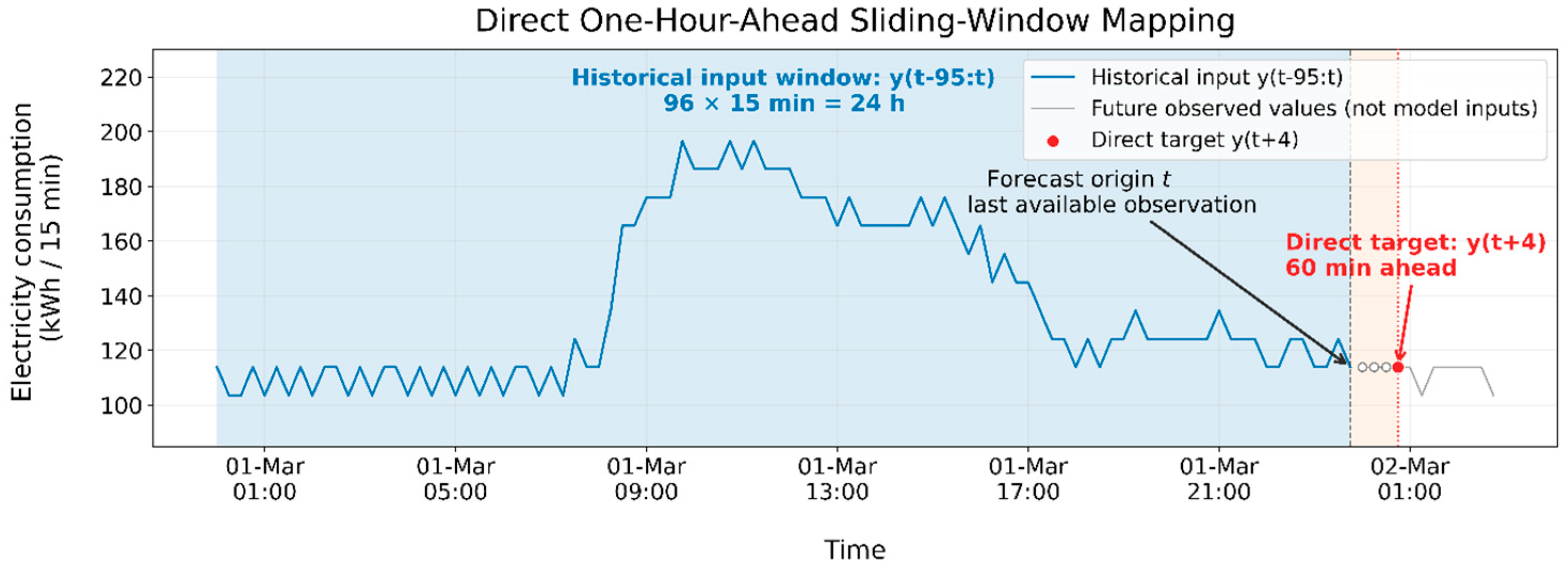
In the study, a sliding window-based sequence generation mechanism was used to learn the temporal dependencies within each fold [31]. Each input sample contains the past 96 time steps. Since the data is recorded at 15 min intervals, the 96 time steps correspond to the last 24 h of observation history. The prediction horizon was determined as 4 time steps. This configuration indicates that the model forecasts electricity consumption one hour ahead using observations from the preceding 24 h. Figure 5 illustrates an example sequence generated from electricity consumption data using a 96-step sliding-window approach. This configuration enables the model to learn daily consumption behavior, calendar-related periodic patterns, short- and long-term temporal dependencies, and nonlinear temporal transitions from information available at the forecast origin.

2.3. SWT-Based Multi-Scale Decomposition

One of the most commonly used methods in signal processing is the Fourier transform. However, the Fourier transform has a significant disadvantage: while frequency information is obtained, time information is lost. Time information is crucial for signals with varying characteristics. This information is necessary for the creation and testing of different systems. Unlike the Fourier transform, wavelet-based methods enable the analysis of time-frequency information in non-stationary signals. This method allows the low- and high-frequency components of a signal to be calculated over a specific time interval. Thus, systems whose frequency changes over time can be examined in more detail. In addition, the analysis of sudden changes can be done more precisely [32]. In the classical wavelet transform, downsampling is performed at each level while the signal is separated into low- and high-frequency components. Therefore, the length of the subbands obtained is reduced. In SWT, however, downsampling is not performed. Therefore, the components obtained at each separation level remain the same length as the original signal. This allows SWT to more accurately capture sudden changes in electricity consumption and local fluctuations [33].

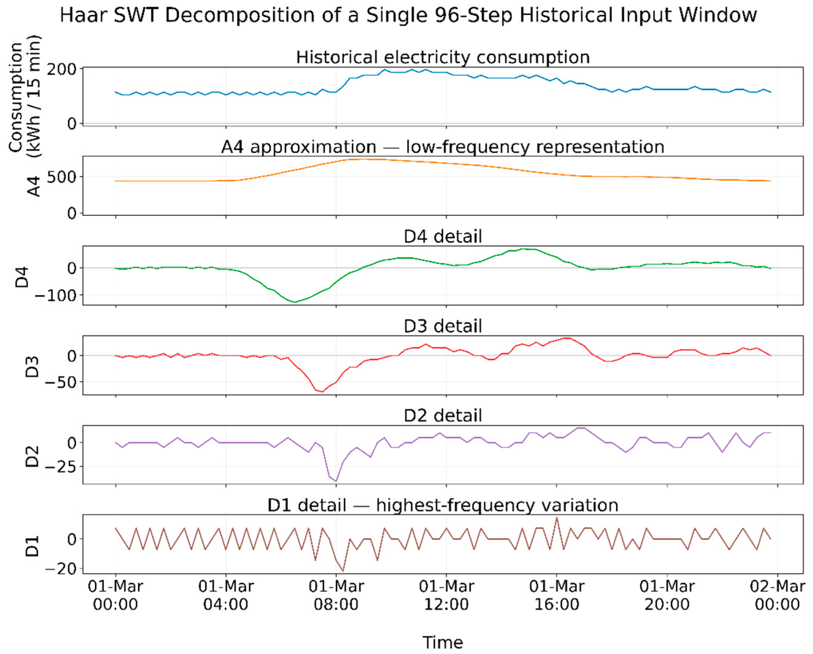
One of the core components of the proposed method is the SWT-based multi-scale signal decomposition approach. Accordingly, the raw time series were not directly fed into the model. Instead, each variable was decomposed into subcomponents representing different frequency resolutions. The SWT transformation was applied at the fourth level. In the final compact model, only the historical electricity consumption series was decomposed using the fourth-level Haar SWT. This decomposition produced five temporally aligned components, namely A4, D4, D3, D2, and D1. Hour and day of week were incorporated as calendar features and were not subjected to SWT decomposition. Thus, the final model uses five SWT-derived consumption components together with two calendar features. Furthermore, different mother wavelets of the SWT were used in the study, and the transformation that yielded the best result was obtained from the Haar mother wavelet. The subcomponents obtained from the SWT signal decomposition are given in Figure 6.

The features obtained after SWT may exhibit different amplitude ranges and statistical distributions. In particular, the approximation and detail components can produce values at substantially different scales depending on the frequency bands they represent. This may cause the model to be disproportionately influenced by features with large numerical magnitudes, while failing to adequately learn low-amplitude variations that may nevertheless be important for forecasting. Therefore, Z-score standardization was applied to all input features before they were introduced into the model [34,35]. Z-score standardization transforms each feature to have a mean of zero and a standard deviation of one. Consequently, features derived from different variables and SWT sub-bands are mapped onto a common scale.

To prevent data leakage, standardization parameters were calculated only from training data. Test data were transformed using the mean and standard deviation values obtained from the training data. In this way, the transfer of distributional information from the test period to the training process is prevented. The standardization process ensures more balanced learning of the model and increases the stability of the training process. It also contributes to the more orderly progress of the gradient-based optimization process and improves the convergence performance [36,37]. The equation for z-score normalization used in the study is given in Equation (2).

$$z={\displaystyle \frac{x-{\mu }_{train}}{{\sigma }_{train}}}$$

(2)

In Equation (2), $x$ represents the raw feature value, ${\mu }_{train}$ represents the mean of the feature calculated only from the training data, ${\sigma }_{train}$ represents the standard deviation of the feature calculated only from the training data, and $z$ represents the standardized value.

2.4. Frequency Attention Mechanism

Frequency Attention Mechanism is an attention-based approach used to determine the relative importance of different frequency components in signal or time series data during the prediction or classification process. Time series data often consist not only of changes along the time axis, but also include various frequency characteristics such as trend, periodicity, sudden fluctuations, and noise. Therefore, modeling the data only in the time domain may result in insufficient learning of the important information represented by some frequency components. The main purpose of the Frequency Attention Mechanism is to adaptively highlight the components that are more informative in terms of the task, rather than transferring all frequency components to the model with equal importance [38,39,40].

The general equations used for the Frequency Attention Mechanism are given in Equations (3)–(7). In the final compact implementation, for each sample and time step, the five consumption-related SWT components (A4, D4, D3, D2, and D1) are provided to the attention-score network as a five-dimensional vector X. The attention scores are calculated using two successive linear transformations with a Tanh activation function between them, as given in Equation (3).

$$\mathrm{s}={\mathrm{W}}_2\tanh \left({\mathrm{W}}_1\mathrm{X}+{\mathrm{b}}_1\right)+{\mathrm{b}}_2$$

(3)

The calculated attention scores are then normalized across the five SWT frequency scales using the Softmax function, as given in Equation (4).

$${\alpha }_f={\displaystyle \frac{\exp \left(s_f\right)}{{\displaystyle {\sum }_{k=1}^K}\exp \left(s_k\right)}}$$

(4)

Each SWT frequency component is multiplied by its corresponding attention weight, as expressed in Equation (5).

$${\tilde{X}}_f={\alpha }_f{X}_f$$

(5)

The weighted SWT components are subsequently concatenated to obtain the Frequency Attention representation, as shown in Equation (6).

$$X_{FA}=Concat({\tilde{X}}_1, {\tilde{X}}_2,\dots ,{\tilde{X}}_K)$$

(6)

Finally, the Hour and Day-of-Week features, which bypass the Frequency Attention mechanism, are concatenated with the weighted SWT representation to form the final input of the TCN, as given in Equation (7).

$$X_{final}=\mathrm{Concat}\left(X_{FA},X_{Hour},X_{DayOfWeek}\right)$$

(7)

In Equation (3), X denotes the 5-dimensional SWT input vector consisting of A4, D4, D3, D2, and D1, and s denotes the corresponding 5-dimensional attention-score vector. $W1$ and ${\mathrm{W}}_2$ represent the learnable weight matrices of the two linear transformations, while ${\mathrm{b}}_1$ and ${\mathrm{b}}_2$ represent their corresponding bias vectors.

In Equations (4)–(6) $X_f$ denotes the $f$. frequency component, $s_f$ represents the attention score calculated for the corresponding component, and ${\alpha }_f$ denotes the attention weight obtained through the softmax function. ${\tilde{X}}_f$ represents the weighted frequency component, $K$ is the total number of frequency components, and $X_{FA}$ denotes the weighted frequency representation obtained after the Frequency Attention mechanism. In the final compact implementation, K = 5.

The Softmax normalization in Equation (4) is performed independently across the five SWT scales for each sample and each time step. Therefore, the resulting attention weights are frequency-specific, sample-specific, and time-dependent rather than global. Although the learnable parameters of the attention score network are shared across samples and time steps, the attention weights themselves depend on the corresponding five-dimensional SWT input vector. Since SWT is applied only to the electricity consumption signal in the final compact model, the attention mechanism is not variable-specific in the sense of assigning separate attention distributions to multiple input variables. The Hour and Day of Week features bypass the Frequency Attention block and are incorporated only during the final feature fusion operation in Equation (7).

For a batch containing samples with 96 time steps, the Frequency Attention score network receives a tensor of size 96 × 5 as input. At its output, it produces attention scores and weighted SWT representations of the same size. After the two calendar features are added to these representations, the final representation provided to the TCN has a size of 96 × 7. The two 5-to-5 linear transformations contain a total of 60 learnable parameters.

Following the SWT decomposition, the electricity consumption signal is represented by the five subbands A4, D4, D3, D2, and D1. These components are not assumed to contribute equally to the forecasting process. Therefore, the Frequency Attention mechanism adaptively determines their relative importance directly from the input data. Components containing more informative characteristics for a particular sample and time step can consequently receive larger weights. In this manner, the model dynamically emphasizes the SWT scales that are more relevant to the forecasting task while retaining all five weighted components for subsequent processing by the TCN.

The proposed Frequency Attention mechanism differs from existing frequency-aware approaches in both representation and function. FECAM [38] employs a DCT-based channel-attention mechanism to model frequency interdependencies across input channels. In contrast, the proposed method directly assigns learnable importance weights to SWT-derived frequency scales of historical electricity consumption. FEDformer [39] performs frequency-domain modeling within a decomposition-based Transformer architecture using Fourier representations, whereas the proposed block does not rely on Transformer attention or Fourier-domain mode selection. WFTNet [40] combines Fourier and wavelet transforms to capture global and local periodic patterns, respectively. The proposed mechanism instead operates directly on Haar SWT components and applies a lightweight shared scoring network to weight the resulting frequency scales before TCN-based temporal modeling.

2.5. Temporal Convolutional Network (TCN)

TCN is a convolution-based deep learning architecture used to model temporal dependencies in sequential data. Unlike recurrent architectures, TCN learns past patterns in parallel using one-dimensional convolution layers applied along the time axis, rather than processing time steps sequentially. The causal convolution used in the architecture ensures that the model uses only past and present time information during the prediction, thus preventing future information from leaking into the model. Dilated convolution, on the other hand, expands the receptive field by applying the convolution filter at certain intervals and allows for more effective capture of long-term dependencies [41]. The equation used for the dilated convolution operation in the TCN architecture is given in Equation (8).

$$F_{\left(s\right)}={\displaystyle \sum _{i=0}^{k-1}}f\left(i\right). x_{s-d.i}$$

(8)

In Equation (8), $F_{\left(s\right)}$ denotes the convolution output at the time step $s$. $x$ represents the input time series, and $f\left(i\right)$ is the $i$th coefficient of the convolution filter. Here, $k$ denotes the filter size, while $d$ represents the dilation factor. Residual connections facilitate information flow in deep TCN architectures and improve the stability of the training process. Owing to these characteristics, TCNs have been effectively applied to problems such as time series forecasting, energy consumption prediction, sensor data analysis, and the modeling of long-term temporal patterns [42]. The mathematical expression used to define the residual connections in the TCN architecture is presented in Equation (9).

$$o=\varphi \left(x+F\left(x\right)\right)$$

(9)

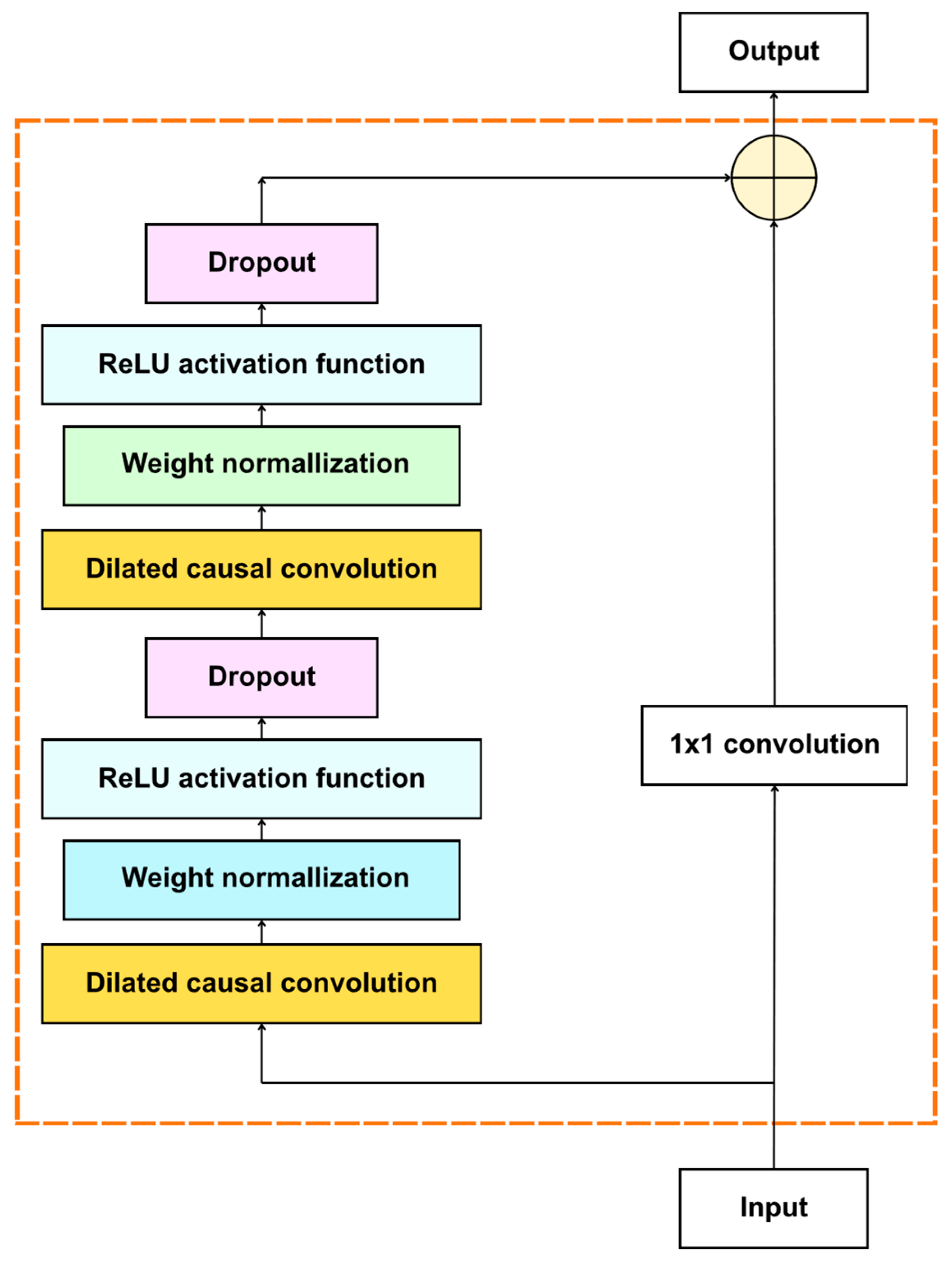
In Equation (9), $o$ denotes the output of the residual block. $x$ represents the input representation fed into the block, $F\left(x\right)$ is the transformation learned by the convolutional layers, and $\varphi \left(.\right)$ denotes the activation function. In the final forecasting stage of the proposed model, a Temporal Convolutional Network (TCN) is employed. TCN further processes the multiscale representations obtained from the preceding layers to capture temporal dependencies. At this stage, the features obtained from the Frequency Attention mechanism were processed along the temporal dimension through the TCN architecture. The dilated convolution structure expands the receptive field of the model, thereby facilitating the learning of relationships across different temporal scales. Consequently, the model can jointly represent both short-term fluctuations and long-term trends in electricity consumption. The causal convolution structure ensures that only past observations are used during the forecasting process, thereby preventing information from future time steps from leaking into the model. Within the proposed framework, the TCN generates one-hour-ahead electricity consumption forecasts using the multiscale feature representations obtained through SWT and the Frequency Attention mechanism. This structure enables the model to simultaneously exploit informative frequency-domain components and temporal dependencies. The fundamental block structure employed within the TCN is illustrated in Figure 7.

2.6. Proposed Model

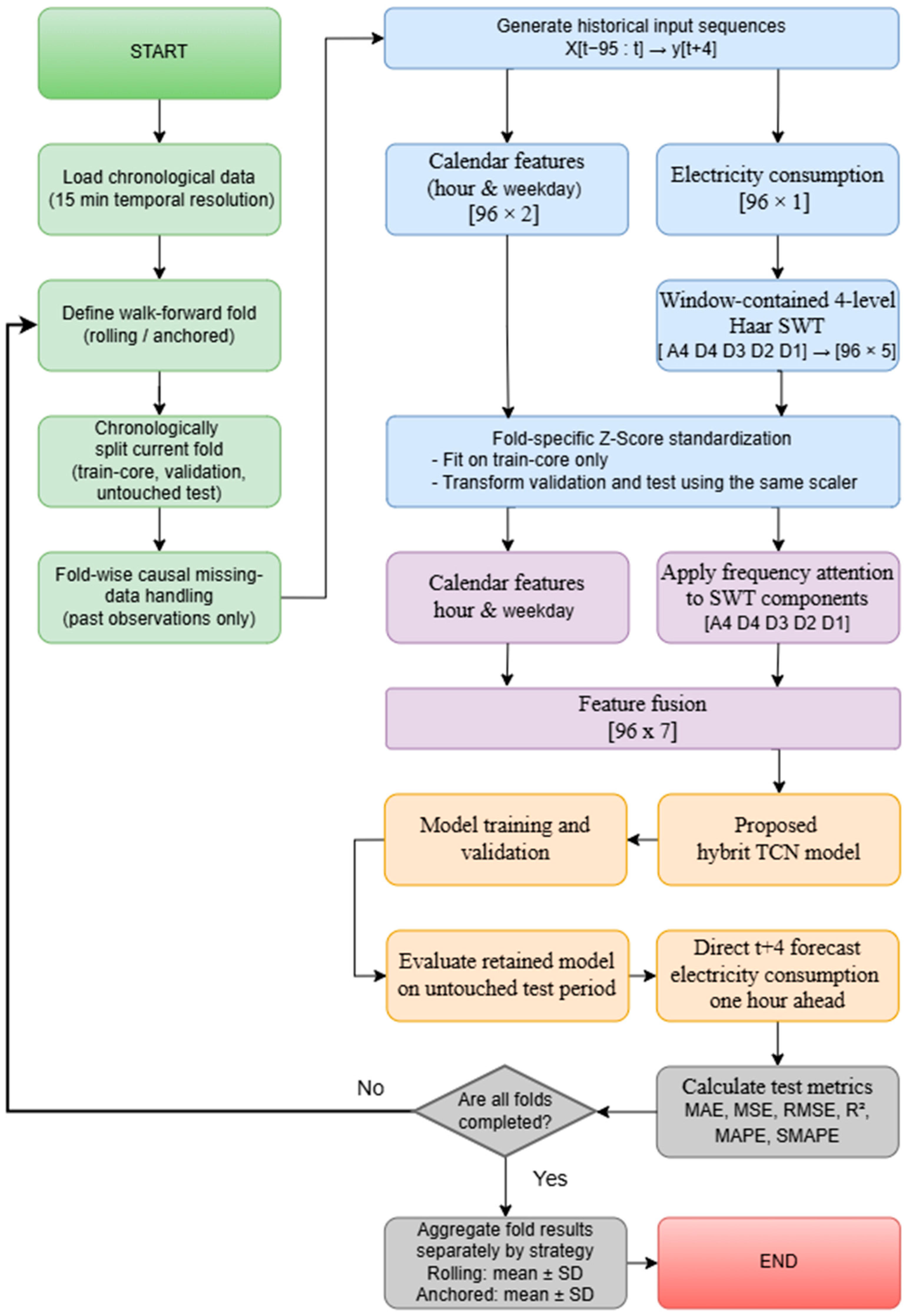
In this phase of the study, a multi-scale prediction model is proposed that utilizes a hybrid structure of SWT, Frequency Attention mechanism, and TCN architecture. The aim of the proposed hybrid model is to decompose the different time-frequency characteristics found in electricity consumption series. Thus, it adaptively highlights the more informative frequency components for prediction and strongly models the temporal dependencies through these components. In this context, instead of directly using the raw time series, the model first decomposes them into multi-resolution frequency components. Then, it learns the importance levels of these components with the attention mechanism and directly predicts the electricity consumption one hour later with the TCN structure.

In the first stage of the proposed architecture, the historical electricity consumption series was subjected to SWT-based multiscale decomposition. Since the SWT method does not involve downsampling, all subcomponents obtained through the decomposition retain the same length as the original signal. In the second stage, a Frequency Attention mechanism was employed to determine the relative importance of the frequency components extracted by SWT in the forecasting process. Rather than assigning equal importance to all frequency components, this mechanism allocates higher weights to those that are more informative for prediction. In this manner, the model can more effectively learn long-term trends and abrupt fluctuations in electricity consumption. In the final stage, the weighted feature representations obtained after the attention mechanism were provided as inputs to the TCN model while preserving the temporal dimension. Within the TCN architecture, causal convolution prevents future information from leaking into the model, whereas dilated convolution enables the learning of long-term temporal dependencies. Accordingly, the proposed SWT + Frequency Attention + TCN model forecasts electricity consumption one hour ahead by jointly exploiting informative frequency domain components and temporal dependencies. This integrated architecture is designed to produce more reliable forecasts for nonlinear, highly variable, and multifactorial time series such as campus electricity consumption. The flowchart of the proposed hybrid model is presented in Figure 8.

Based on the feature ablation results, the final compact forecasting model uses historical electricity consumption together with the calendar variables Hour and Day of Week, which are known at the forecast origin. The historical 96-step electricity consumption sequence is independently decomposed for each input window using a 4-level Haar SWT and transformed into a 96 × 5 multiscale representation consisting of the A4, D4, D3, D2, and D1 components. The Frequency Attention mechanism adaptively reweights these 5 components for each sample and time step. The Hour and Day of Week features are not provided to the attention block. The weighted SWT components are combined with the 2 calendar features using a feature fusion approach. As a result of this operation, the 96 × 7 representation is transformed into channel-first format and provided to the TCN architecture as an input of size 7 × 96.

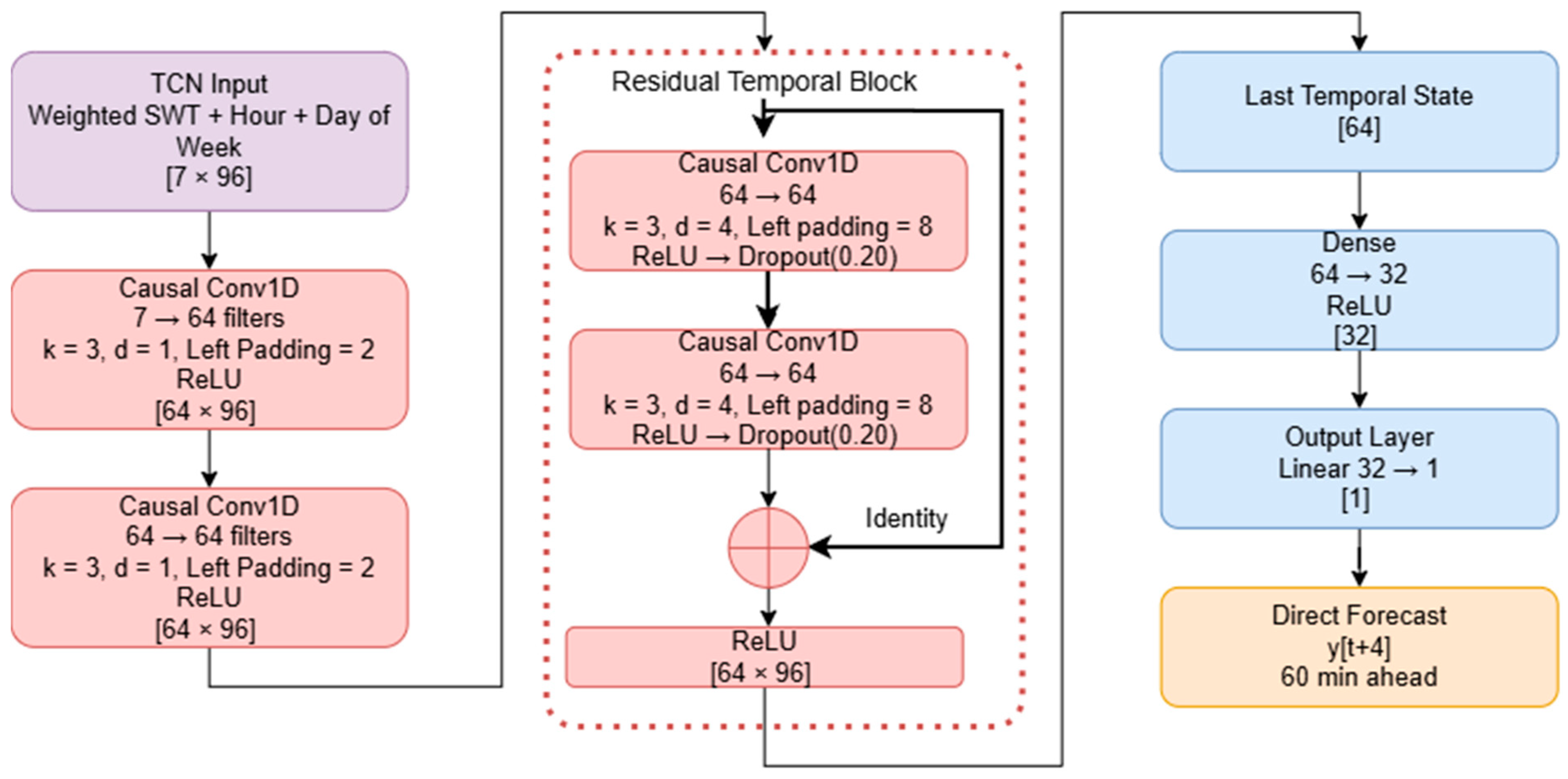
The proposed TCN architecture consists of two initial causal Conv1D layers followed by a single residual temporal block. The first Conv1D layer transforms the 7 input channels into 64 feature channels. The second Conv1D layer operates with 64 input and 64 output channels. Both initial convolutional layers use a kernel size of 3, a dilation value of 1, and the ReLU activation function. Thus, the convolutional representation reaches a size of 64 × 96.

The single residual temporal block following the initial layers consists of 2 causal Conv1D layers. Each of these layers uses 64 filters, a kernel size of 3, and a dilation value of 4. Each convolution is followed by a ReLU activation and a dropout rate of 0.20. The output of the second convolution is combined with the identity connection from the input of the residual block and is then passed through another ReLU activation. Weight normalization was not used in the final implementation.

Strict left-sided causal padding is used in all convolutions to prevent future observations from contributing to the current outputs. A left padding of 2 steps is applied to layers with a dilation value of 1, while a left padding of 8 steps is applied to layers with a dilation value of 4. Since no padding is applied on the right side, future observations are not included in the computation of any convolutional output. Considering the dilation sequence of 1, 1, 4, 4 and a kernel size of 3, the effective receptive field of the TCN is 21 time steps. Given the 15 min temporal resolution of the dataset, this corresponds to 5.25 h of historical context.

The 64-dimensional hidden state corresponding to the final time step of the 64 × 96 representation obtained at the end of the residual block is transferred to the forecasting head. The forecasting head first includes a fully connected layer from 64 to 32 dimensions followed by a ReLU activation, and then a linear output layer from 32 to 1 dimension. Thus, the model produces a single scalar output, which directly represents y_t+4, in other words, electricity consumption 60 min after the final observation.

The proposed SWT + Frequency Attention + TCN architecture contains a total of 40,637 learnable parameters. Since SWT is a deterministic transformation, it contains no learnable parameters, whereas the two 5-to-5 linear layers in the Frequency Attention block add a total of 60 parameters. The layer structure, tensor dimensions, dilation and padding settings, residual connection, and forecasting head of the proposed model are illustrated in detail in Figure 9.

To prevent information leakage, the transformation operations were performed strictly within the boundaries of each historical input sequence. Each 96-step input window was independently decomposed using SWT; therefore, no observations occurring after the corresponding forecast origin were involved in the computation of the SWT coefficients. Standardization was performed independently for each temporal fold and model development run. The standard scaler parameters were estimated exclusively from the train core set and then applied unchanged to the corresponding validation and test observations. Therefore, no information regarding the mean or variance of the validation or test distributions was introduced into the model training process. No target time meteorological observations or external weather forecasts are required. The model performs direct single output forecasting. Specifically, when the last observation in the historical input sequence corresponds to time, the model predicts only y_t+4. Since the temporal resolution of the dataset is 15 min, this target corresponds to exactly 60 min ahead of the forecast origin. Therefore, the intermediate t + 1, t + 2, and t + 3 values are neither recursively predicted nor simultaneously generated as model outputs. To evaluate model performance more accurately under real-world forecasting conditions, a walk-forward validation approach was employed instead of a conventional random train–test split. For the first prediction in each test period, the required 96-step historical context was constructed using only observations available before the test boundary. Thus, no future test observations were included as inputs when generating the first forecast of the test period. The training hyperparameters and validation settings used for the proposed model are summarized in

Table 3. Training hyperparameters and validation settings of the proposed model.

Hyperparameters	Values
Maximum Epoch	200
Early stopping patience	30 epochs
Train-core subset	First 85% of each outer training fold
Validation split	Last 15% of each outer training fold
Test window	Subsequent 10% of the total time series
Validation criterion	Validation MSE loss
Scaler fitting	Train-core only
Test-set use	Final evaluation only
Batch size	64
Learning rate	0.001
Optimizer	Adam
Loss	MSE
Wavelet	haar
Wavelet level	4

. In addition, the performance of the proposed model was compared with that of several deep learning models. To ensure a fair comparison, the same fold structure and data preprocessing procedure were used across all individual models and hybrid architectures.

2.7. Experimental Verification and Ablation Analysis

To provide a comprehensive assessment of the proposed model, the experimental comparison was extended beyond conventional deep learning architectures to include forecasting methods with different modeling principles and levels of complexity. The benchmark set comprised last value, daily, and weekly persistence models, Random Forest, XGBoost, SARIMA, Informer, XGBoost + LSTM, and AutoReg Ridge architectures. In addition, SWT-based and SWT + Frequency Attention-based variants of the deep learning models were evaluated. This benchmark design enables the proposed method to be assessed against simple seasonal baselines, autoregressive approaches, tree-based machine learning methods, conventional deep learning architectures, and a contemporary Transformer-based forecasting approach under the same temporal evaluation framework. All trainable models were evaluated using the same chronological validation framework, while model-specific configurations were selected using a comparable validation-based model selection procedure.

Because deep learning architectures have different capacity and optimization characteristics, a model-specific configuration approach was adopted instead of using the same architectural hyperparameters for all models. The architectural configurations of LSTM, BiLSTM, CNN LSTM, TCN, and the other models were evaluated under the same chronological validation procedure and a comparable search budget. The first 85% of each outer training fold was used as the train core set, while the last 15% was used as the validation set, and only validation performance was considered during model selection. The test periods were not included in hyperparameter selection. The selected model-specific configurations were subsequently used without modification in the rolling and anchored walk-forward evaluations.

To further improve the transparency and reproducibility of the experimental comparison, the main architecture-specific configurations and model complexities of the evaluated forecasting models are summarized in

Table 4. Architecture-specific configurations and model complexity of the evaluated forecasting models.

Model	Main Architecture-Specific Configuration	Model Complexity
Proposed model	2 causal Conv1D layers (64 filters, k = 3, d = 1) 1 residual block (2 causal Conv1D layers (64 filters, k = 3, d = 4, dropout = 0.20)) Dense 64–32–1	40,637 trainable parameters
SWT + FA + LSTM	1-layer LSTM (hidden = 64) Dense 64–32–1	20,861 trainable parameters
SWT + FA + BiLSTM	1-layer BiLSTM (hidden = 64 per direction) Dense 128–32–1	41,597 trainable parameters
SWT + FA + CNN-LSTM	2 Conv1D (64 filters, k = 3) 1-layer LSTM (hidden = 64) Dense 64–32–1	49,213 trainable parameters
CNN-BiGRU-Attention	CNN + bidirectional GRU + attention + regression head	75,393 trainable parameters
Informer	Transformer-based Informer architecture	11,309,569 trainable parameters
XGBoost + LSTM	XGBoost feature modeling + LSTM forecasting component	XGBoost + 19,777 neural parameters
XGBoost	Gradient-boosted decision-tree ensemble	Tree-based complexity
Random Forest	Random-forest ensemble	Tree-based complexity
AutoReg-Ridge	Autoregressive linear model with Ridge regularization	Fitted linear coefficients
SARIMA	SARIMA(1,0,1) × (1,0,0,96)	Estimated statistical coefficients
Last Persistence	Previous available observation	0 trainable parameters
Daily Persistence	Observation from the same time one day earlier	0 trainable parameters
Weekly Persistence	Observation from the same time one week earlier	0 trainable parameters

. Trainable parameter counts are reported for neural network-based models. For tree-based and statistical approaches, model complexity is described in terms of the corresponding model structure because their fitted numbers of nodes or coefficients are not directly comparable with the trainable parameter counts of neural networks.

To ensure experimental reproducibility, a fixed random seed of 42 was used for the primary controlled experiments, with the random states of Python 3.10.19, NumPy 2.2.5, and PyTorch 2.12.0 set consistently. The main comparative experiments were performed once per walk-forward fold using this fixed seed. In addition, the robustness of the final SWT + Frequency Attention + TCN model to random initialization was examined using three seeds (42, 52, and 62). Each seed was evaluated over four rolling and four anchored walk-forward folds, resulting in 24 fold-level training and evaluation runs for the seed robustness analysis. All experimental studies were conducted on a desktop computer equipped with 32 GB of RAM, an Intel Core Ultra 7 265KF processor, and an NVIDIA GeForce RTX 5060 GPU with 8 GB of memory. The experiments were performed using the Python programming language in an Anaconda environment on the Windows 11 operating system.

In the ablation analysis, SWT-based multiscale feature extraction was initially applied to the deep learning models. This allowed the prediction performance of different deep learning architectures to be compared under the same frequency representation. In this study, CNN LSTM, LSTM, BiLSTM, and TCN models were tested using multiscale input features obtained with SWT. Thus, the functionality of the SWT-based representation with different temporal modeling structures was investigated. As part of the feature ablation analysis, the contribution of meteorological variables was also examined. Although temperature, humidity, wind speed, atmospheric pressure, and solar irradiance were available in the original dataset, their inclusion did not provide any additional improvement in forecasting accuracy compared with the configuration based on historical electricity consumption and calendar variables. Accordingly, the final compact model was defined using only historical electricity consumption, Hour, and Day of Week. This configuration was subsequently used for the final model evaluation. Importantly, the final model does not require target time meteorological observations or external weather forecasts.

In addition, a mother wavelet sensitivity analysis was conducted using only the model development validation data. The analysis showed that the Haar wavelet provided the best validation performance among the evaluated candidates. Under the same decomposition level, number of input features, and model complexity, Haar achieved the lowest validation MAE (7.759 ± 0.090) and RMSE (11.373 ± 0.255), together with the highest R² (0.9410 ± 0.0026). In comparison, coif1 yielded an RMSE of 12.225 ± 0.671, while db2 and sym2 both resulted in an RMSE of 13.662 ± 0.387. Based on these validation results, Haar was retained as the mother wavelet of the proposed model. The results of the wavelet and decomposition level sensitivity analysis conducted before the full-set ablations are presented in

Table 5. Wavelet- and decomposition-level sensitivity analysis conducted before the full-set ablations.

Mother Wavelet	Level	Input Features	Val. MAE ± SD	Val. RMSE ± SD	Val. R2 ± SD
haar	4	32	7.759 ± 0.090	11.373 ± 0.255	0.9410 ± 0.0026
coif1	4	32	8.511 ± 0.472	12.225 ± 0.671	0.9317 ± 0.0076
db2	4	32	9.493 ± 0.344	13.662 ± 0.387	0.9149 ± 0.0048
sym2	4	32	9.493 ± 0.344	13.662 ± 0.387	0.9149 ± 0.0048

.

Secondly, to determine the contribution of the Frequency Attention mechanism to prediction performance, each SWT-based model was compared between a version without the attention mechanism and a version with Frequency Attention added. This experimental group was designed to reveal whether the proposed frequency attention mechanism contributes to performance not only on the TCN architecture but also on different deep learning models.

Thirdly, the impact of the TCN architecture within the proposed structure was examined comparatively with other deep learning models. Thanks to its causal and extensional convolutional structure, TCN can effectively model dependencies in past time steps. Therefore, using multi-scale frequency representations obtained with SWT within the TCN structure allows for the simultaneous learning of both short-term consumption fluctuations and longer-term temporal patterns.

Fourth, the generalization capability of the proposed model under different time-based validation conditions was evaluated using rolling walk-forward and anchored walk-forward strategies. In the rolling walk-forward strategy, the training window was advanced along the time axis to test the model’s capacity to adapt to more recent consumption patterns. In the anchored walk-forward strategy, the training window was extended from the initial date to examine the model’s learning performance with accumulated past information. The combined use of rolling and anchored walk-forward strategies enabled the temporal robustness of the proposed model to be evaluated under two different validation schemes applied to the same campus electricity consumption record.

2.8. Performance Evaluation Metrics

Five different evaluation metrics were used to compare the performance of the forecasting models. Mean Absolute Error (MAE) represents the average magnitude of the absolute prediction errors. Mean Squared Error (MSE) is calculated as the average of the squared prediction errors. Root Mean Squared Error (RMSE) is the square root of MSE and places greater emphasis on large prediction errors. Therefore, it makes substantial deviations more apparent under conditions involving sudden load peaks, peak demand, or highly fluctuating electricity consumption. Mean Absolute Percentage Error (MAPE) expresses the prediction error as a percentage and is useful for comparing model performance across datasets or variables with different scales. Symmetric Mean Absolute Percentage Error (SMAPE) provides a more symmetric percentage-based error measure than MAPE and generally yields more balanced results when the actual values are close to zero [43,44]. Coefficient of Determination ${(\mathrm{R}}^2)$ indicates the extent to which the model explains the variation in the actual data. As it approaches 1, the explanatory power of the model increases [45]. The performance evaluation criteria used in the study are given in

Table 6. Performance Metrics.

Metrics	Equation
MAE	$\mathrm{M}\mathrm{A}\mathrm{E}={\displaystyle \frac{1}{\mathrm{N}}}{\displaystyle \sum _{\mathrm{i}=1}^{\mathrm{N}}}\left|\right({\mathrm{Y}}_{\mathrm{i}}-{\widehat{\mathrm{Y}}}_{\mathrm{i}})|$
MSE	$\mathrm{M}\mathrm{S}\mathrm{E}={\displaystyle \frac{1}{\mathrm{N}}}{\displaystyle \sum _{\mathrm{i}=1}^{\mathrm{N}}}{\left({\mathrm{Y}}_{\mathrm{i}}-{\widehat{\mathrm{Y}}}_{\mathrm{i}}\right)}^2$
RMSE	$\mathrm{R}\mathrm{M}\mathrm{S}\mathrm{E}=\sqrt{{\displaystyle \frac{1}{\mathrm{N}}}}{\displaystyle \sum _{\mathrm{i}=1}^{\mathrm{N}}}{{(\mathrm{Y}}_{\mathrm{i}}-{\widehat{\mathrm{Y}}}_{\mathrm{i}})}^2$
MAPE	$\mathrm{M}\mathrm{A}\mathrm{P}\mathrm{E}={\displaystyle \frac{100}{\mathrm{N}}}{\displaystyle \sum _{\mathrm{i}=1}^{\mathrm{N}}}|{\displaystyle \frac{{\mathrm{Y}}_{\mathrm{i}}-{\widehat{\mathrm{Y}}}_{\mathrm{i}}}{{\mathrm{Y}}_{\mathrm{i}}}}|$
SMAPE	$\mathrm{S}\mathrm{M}\mathrm{A}\mathrm{P}\mathrm{E}={\displaystyle \frac{100}{\mathrm{N}}}{\displaystyle \sum _{\mathrm{i}=1}^{\mathrm{N}}}{\displaystyle \frac{{2|\mathrm{Y}}_{\mathrm{i}}-{\widehat{\mathrm{Y}}}_{\mathrm{i}}|}{\left|{\mathrm{Y}}_{\mathrm{i}}\right|+|{\widehat{\mathrm{Y}}}_{\mathrm{i}}|}}$
${\mathrm{R}}^2$	${\mathrm{R}}^2=1-{\displaystyle \frac{{\displaystyle {\sum }_{\mathrm{i}=1}^{\mathrm{N}}}{{(\mathrm{Y}}_{\mathrm{i}}-{\widehat{\mathrm{Y}}}_{\mathrm{i}})}^2}{{\displaystyle {\sum }_{\mathrm{i}-1}^{\mathrm{N}}}{{(\mathrm{Y}}_{\mathrm{i}}-\overline{Y})}^2}}$

. In Table 6, $Y_i$ represents the actual value, and ${\widehat{\mathrm{Y}}}_{\mathrm{i}}$ represents the predicted value. $N$ is the sample size, and $A_i$ is the average of the actual values.

3. Prediction Results

In this study, the contributions of the different components and input variables of the proposed model to forecasting performance were examined separately. First, the effects of the SWT-based multiscale representation and the Frequency Attention mechanism were evaluated using the full dataset. To assess the independent contribution of SWT, the performance of the proposed TCN model on raw data was also tested in addition to the SWT + TCN and SWT + Frequency Attention + TCN configurations. Subsequently, the contribution of the input variables was evaluated through feature ablation analysis, and the final compact input configuration was determined based on the results of this analysis. The subsequent comprehensive benchmark comparisons and robustness analyses were then conducted using this compact input configuration.

The rolling walk-forward results show that the SWT and Frequency Attention components contribute separately to the TCN backbone. While the Raw TCN model achieved an RMSE of 13.336, the addition of the SWT-based multiscale representation reduced the RMSE to 13.075. Adding the Frequency Attention mechanism to the SWT representation further reduced the RMSE to 12.295. Accordingly, SWT provided an improvement of approximately 1.96% in RMSE compared with the Raw TCN, while Frequency Attention provided an additional improvement of approximately 5.97% compared with SWT + TCN. The complete SWT + Frequency Attention + TCN configuration achieved an overall RMSE reduction of approximately 7.81% compared with the Raw TCN. In addition, Frequency Attention was observed to reduce the error values of the SWT-based LSTM, BiLSTM, and CNN LSTM models.

The anchored walk-forward evaluation confirms the same trend in component contributions. The Raw TCN model achieved an RMSE of 12.936, which decreased to 12.446 with the SWT + TCN configuration and further decreased to 11.800 with the SWT + Frequency Attention + TCN configuration. Accordingly, the use of SWT reduced RMSE by approximately 3.79% compared with the Raw TCN. The addition of the Frequency Attention mechanism to the SWT representation provided a further improvement of approximately 5.19% in RMSE. The transition from the Raw TCN to the complete SWT + Frequency Attention + TCN configuration resulted in an overall RMSE reduction of approximately 8.78%. When the rolling and anchored walk-forward results are considered together, the performance improvement is not solely attributable to the Frequency Attention mechanism. The SWT-based multiscale representation also provides an independent and complementary contribution to forecasting performance.

A feature ablation analysis was conducted to identify variables that were unnecessary or provided only limited contributions and to determine the final input configuration to be used in the subsequent comprehensive benchmark experiments. In this analysis, historical electricity consumption, meteorological variables, and the Hour and Day of Week calendar variables were evaluated under different combinations. Thus, the contribution of each variable group to forecasting performance was examined separately.

The feature ablation results showed that adding meteorological variables to historical consumption information did not improve forecasting performance for this dataset. The Consumption + Weather configuration produced higher error values than the consumption-only configuration under both walk-forward strategies. In contrast, adding the Hour and Day of Week variables to historical consumption information provided a clear improvement in performance. The Consumption + Calendar configuration achieved the best results among the evaluated input combinations, with an RMSE of 10.614 ± 1.042 under the rolling evaluation and 10.286 ± 1.330 under the anchored evaluation. Based on these findings, the final compact input configuration was defined as historical electricity consumption, Hour, and Day of Week. Meteorological variables were not included in the subsequent experiments.

The same compact input configuration was used in all benchmark, robustness, and additional evaluation experiments conducted after this stage. All models were evaluated using the same forecasting target, rolling and anchored test periods, and temporal evaluation framework. Where required by the model architecture, the input representation was adapted to the corresponding model, while the information available to the models remained unchanged. Thus, the comparisons were conducted under a common information budget.

The performance of the proposed SWT + Frequency Attention + TCN model was compared with a broad benchmark group representing different modeling approaches. This group included persistence and autoregressive methods, machine learning models, Informer, conventional deep learning architectures, and SWT-based hybrid structures. All models were evaluated using the MAE, MSE, RMSE, MAPE, SMAPE, and R² metrics under the same rolling and anchored walk-forward evaluation framework. Thus, the performance of the proposed model was compared not only with similar deep learning architectures but also with methods representing different forecasting paradigms. The rolling walk-forward results are presented in

Table 7. Full-set ablation results under rolling walk-forward evaluation.

Model	MAE	MSE	RMSE	MAPE	SMAPE	R2
SWT + LSTM	10.228 ± 1.488	252.113 ± 108.687	15.878 ± 3.249	7.482 ± 0.465	7.305 ± 0.490	0.883 ± 0.040
SWT + FA + LSTM	8.635 ± 0.610	168.814 ± 42.197	12.993 ± 1.619	6.607 ± 0.698	6.369 ± 0.575	0.922 ± 0.026
SWT + BiLSTM	9.907 ± 1.066	223.572 ± 64.715	14.952 ± 2.117	7.365 ± 0.468	7.149 ± 0.420	0.896 ± 0.031
SWT + FA + BiLSTM	8.496 ± 0.433	166.427 ± 36.964	12.901 ± 1.453	6.466 ± 0.684	6.263 ± 0.571	0.923 ± 0.030
SWT + CNN-LSTM	9.601 ± 1.232	216.070 ± 74.857	14.699 ± 2.505	7.144 ± 0.434	6.997 ± 0.301	0.900 ± 0.030
SWT + FA + CNN-LSTM	8.748 ± 0.390	177.453 ± 38.333	13.321 ± 1.443	6.616 ± 0.599	6.431 ± 0.469	0.918 ± 0.030
Raw TCN	8.865 ± 0.749	180.202 ± 48.777	13.336 ± 1.768	6.792 ± 0.836	6.550 ± 0.622	0.909 ± 0.037
SWT + TCN	8.750 ± 0.530	170.948 ± 34.935	13.075 ± 1.341	6.752 ± 0.651	6.522 ± 0.476	0.921 ± 0.027
SWT + FA + TCN	8.238 ± 0.293	151.160 ± 23.728	12.295 ± 0.965	6.346 ± 0.406	6.153 ± 0.285	0.930 ± 0.023

.

Table 7 presents the campus electricity consumption forecasting performance of the models evaluated under the rolling walk-forward validation strategy using the final compact input configuration. The results are reported as mean ± standard deviation across the four test folds. Overall, forecasting errors decrease substantially when moving from persistence-based methods to statistical and machine learning-based models. The Daily Persistence model produced the highest forecasting error, with an RMSE of 35.644 ± 3.326 and an R² of 0.3784 ± 0.0714, while the RMSE decreased to 28.246 ± 6.907 for Weekly Persistence and to 18.206 ± 1.982 for Last Persistence. These results indicate that historical consumption observations contain important information for forecasting. However, they also show that persistence methods based on the direct repetition of these values are not sufficient on their own to capture the more complex temporal patterns in campus electricity consumption.

Among the statistical models, SARIMA achieved an RMSE of 15.813 ± 1.563 and an R² of 0.8778 ± 0.0140, while the AutoReg Ridge model reduced the RMSE to 13.493 ± 1.136. The more advanced benchmark models further reduced the forecasting errors. The Informer model achieved an RMSE of 11.891 ± 0.630 and an R² of 0.9297 ± 0.0141. XGBoost + LSTM, XGBoost, and Random Forest showed similarly strong forecasting performance, with RMSE values of 11.181 ± 1.510, 11.164 ± 1.526, and 11.146 ± 1.534, respectively. These results indicate that tree-based ensemble methods can also provide competitive performance against advanced neural network-based models for campus electricity consumption forecasting.

The proposed SWT + Frequency Attention + TCN model achieved an MAE of 7.074 ± 0.238, an MSE of 113.479 ± 21.968, an RMSE of 10.614 ± 1.042, a MAPE of 5.569 ± 0.575%, a SMAPE of 5.402 ± 0.494%, and an R² of 0.9420 ± 0.0211 under the rolling evaluation. With these results, the proposed model achieved the lowest mean MAE, MSE, RMSE, MAPE, and SMAPE values among the methods presented in Table 10, while also achieving the highest mean R² value. Compared with Random Forest, one of the strongest alternatives, the mean RMSE decreased from 11.146 to 10.614, corresponding to a reduction of approximately 4.77%. Compared with the Last Persistence model, the mean RMSE was reduced by approximately 41.7%.

The performance of the proposed model can be attributed to the complementary contributions of the SWT, Frequency Attention, and TCN components. SWT enables the decomposition of campus electricity consumption into patterns at different time and frequency scales, while the Frequency Attention mechanism selectively weights the frequency components that are more informative for forecasting. The TCN then captures short- and long-term temporal dependencies within these enhanced representations. Therefore, the integration of multiscale decomposition, adaptive frequency selection, and temporal feature extraction provides an effective framework for campus electricity consumption forecasting. The results obtained using the anchored walk-forward validation technique are presented in

Table 8. Full-set ablation results under anchored walk-forward evaluation.

Model	MAE	MSE	RMSE	MAPE	SMAPE	R2
SWT + LSTM	9.479 ± 1.934	226.434 ± 122.208	15.048 ± 3.733	6.888 ± 0.718	6.744 ± 0.814	0.895 ± 0.044
SWT + FA + LSTM	8.285 ± 1.000	169.500 ± 67.244	13.019 ± 2.620	6.245 ± 0.672	6.034 ± 0.502	0.921 ± 0.038
SWT + BiLSTM	9.509 ± 1.323	216.062 ± 69.098	14.699 ± 2.288	7.059 ± 0.566	6.851 ± 0.569	0.900 ± 0.030
SWT + FA + BiLSTM	8.291 ± 0.662	160.021 ± 36.492	12.650 ± 1.459	6.292 ± 0.594	6.092 ± 0.452	0.926 ± 0.027
SWT + CNN-LSTM	9.694 ± 1.450	227.315 ± 76.510	15.077 ± 2.576	7.061 ± 0.793	6.915 ± 0.588	0.894 ± 0.035
SWT + FA + CNN-LSTM	8.582 ± 0.858	169.392 ± 54.413	13.015 ± 2.098	6.468 ± 0.822	6.267 ± 0.575	0.921 ± 0.035
Raw TCN	8.566 ± 0.686	169.085 ± 37.625	12.936 ± 1.524	6.486 ± 0.448	6.329 ± 0.243	0.917 ± 0.022
SWT + TCN	8.351 ± 0.913	154.901 ± 49.617	12.446 ± 2.017	6.466 ± 0.618	6.223 ± 0.459	0.928 ± 0.028
SWT + FA + TCN	7.887 ± 0.771	139.236 ± 43.311	11.800 ± 1.842	6.060 ± 0.676	5.893 ± 0.469	0.935 ± 0.028

.

Table 8 presents the forecasting performance of the models under the anchored walk-forward validation strategy. The persistence-based models show the lowest performance, with Daily Persistence achieving an RMSE of 35.644 ± 3.326 and an R² of 0.3784 ± 0.0714. The Last Persistence model performs considerably better, with an RMSE of 18.206 ± 1.982 and an R² of 0.8384 ± 0.0160, confirming the strong temporal dependence of campus electricity consumption. Among the statistical and autoregressive models, SARIMA achieves an RMSE of 15.871 ± 1.645 and an R² of 0.8770 ± 0.0136, while AutoReg Ridge further reduces the RMSE to 13.483 ± 1.161 and increases the R² to 0.9100 ± 0.0189. Among the more advanced benchmark models, Informer achieves an RMSE of 11.123 ± 1.777 and an R² of 0.9379 ± 0.0213. Random Forest, XGBoost + LSTM, and XGBoost provide stronger results, with RMSE values of 10.909 ± 1.860, 10.861 ± 1.780, and 10.869 ± 1.841, respectively. These results demonstrate the competitiveness of machine learning and hybrid approaches for campus electricity consumption forecasting.

The best overall performance is obtained by SWT + Frequency Attention + TCN, which achieves an MAE of 6.863 ± 0.339, an MSE of 107.125 ± 27.488, an RMSE of 10.286 ± 1.330, a MAPE of 5.311 ± 0.266%, a SMAPE of 5.205 ± 0.173%, and an R² of 0.9463 ± 0.0191. Compared with the strongest benchmark, XGBoost + LSTM, the proposed model reduces the RMSE from 10.861 ± 1.780 to 10.286 ± 1.330, corresponding to an improvement of approximately 5.29%, while increasing the R² from 0.9414 ± 0.0173 to 0.9463 ± 0.0191. When Tables 10 and 11 are evaluated together, the proposed SWT + Frequency Attention + TCN model achieves the lowest mean forecasting errors and the highest mean R² under both rolling and anchored walk-forward validation strategies. The slightly lower error values and higher R² obtained under the anchored strategy suggest that the expanding training dataset may contribute to improved model learning. These findings support the temporal robustness of the proposed approach across the two validation settings applied to the same campus dataset.

In addition to the main forecasting performance, the computational cost of the proposed SWT + Frequency Attention + TCN model was also evaluated. The model contains only 40,637 trainable parameters. The mean training time was approximately 174.59 s per fold under the anchored walk-forward strategy and 123.86 s per fold under the rolling walk-forward strategy. The mean inference time for an entire test fold was approximately 0.091 s and 0.083 s, respectively, corresponding to approximately 0.022 ms and 0.020 ms per sample. These results indicate that the proposed compact architecture can rapidly generate one-hour-ahead forecasts with a low inference cost.

In addition to the main performance metrics, paired statistical comparisons were conducted to evaluate whether the observed error differences were consistent across forecasting samples. In Table 7, Table 8,

Table 9. Feature ablation results used to determine the final compact input configuration.

Strategy	Feature Configuration	Active Transformed Features	MAE	MSE	RMSE	MAPE	SMAPE	R2
Rolling	Consumption only	5	7.482 ± 0.298	137.833 ± 19.149	11.718 ± 0.842	5.758 ± 0.166	5.633 ± 0.230	0.9317 ± 0.0150
	Consumption + Calendar	7	7.074 ± 0.238	113.479 ± 21.968	10.614 ± 1.042	5.569 ± 0.575	5.402 ± 0.494	0.9420 ± 0.0211
	Consumption + Weather	30	8.672 ± 0.150	171.726 ± 16.893	13.093 ± 0.643	6.661 ± 0.431	6.442 ± 0.356	0.9137 ± 0.0236
	Full model	32	8.238 ± 0.293	151.160 ± 23.728	12.295 ± 0.965	6.346 ± 0.406	6.153 ± 0.285	0.930 ± 0.023
Anchored	Consumption only	5	7.399 ± 0.412	134.565 ± 25.775	11.557 ± 1.158	5.707 ± 0.138	5.570 ± 0.136	0.9337 ± 0.0162
	Consumption + Calendar	7	6.863 ± 0.339	107.125 ± 27.488	10.286 ± 1.330	5.311 ± 0.266	5.205 ± 0.173	0.9463 ± 0.0191
	Consumption + Weather	30	8.078 ± 0.539	152.697 ± 27.010	12.318 ± 1.140	6.127 ± 0.186	5.987 ± 0.132	0.9248 ± 0.0165
	Full model	32	7.887 ± 0.771	139.236 ± 43.311	11.800 ± 1.842	6.060 ± 0.676	5.893 ± 0.469	0.935 ± 0.028

,

Table 10. Final benchmark comparison under rolling walk-forward evaluation using the compact input configuration.

Model	MAE	MSE	RMSE	MAPE	SMAPE	R2
Daily Persistence	18.117 ± 1.035	1278.779 ± 231.555	35.644 ± 3.326	12.963 ± 0.267	12.461 ± 0.212	0.3784 ± 0.0714
Weekly Persistence	16.451 ± 4.556	833.636 ± 420.245	28.246 ± 6.907	11.717 ± 4.345	11.269 ± 4.231	0.5454 ± 0.3473
Last Persistence	10.660 ± 1.000	334.390 ± 72.073	18.206 ± 1.982	7.525 ± 0.278	7.512 ± 0.337	0.8384 ± 0.0160
SARIMA	9.841 ± 0.761	251.886 ± 48.234	15.813 ± 1.563	7.085 ± 0.244	7.042 ± 0.272	0.8778 ± 0.0140
AutoReg-Ridge	8.830 ± 0.563	183.033 ± 29.537	13.493 ± 1.136	6.744 ± 0.242	6.685 ± 0.253	0.9098 ± 0.0193
Informer	7.902 ± 0.464	141.688 ± 14.859	11.891 ± 0.630	6.110 ± 0.479	5.925 ± 0.455	0.9297 ± 0.0141
XGBoost + LSTM	7.379 ± 0.596	126.718 ± 33.978	11.181 ± 1.510	5.656 ± 0.325	5.507 ± 0.294	0.9372 ± 0.0189
XGBoost	7.401 ± 0.603	126.389 ± 34.381	11.164 ± 1.526	5.657 ± 0.317	5.520 ± 0.296	0.9374 ± 0.0186
Random Forest	7.359 ± 0.701	125.996 ± 35.010	11.146 ± 1.534	5.630 ± 0.381	5.490 ± 0.361	0.9378 ± 0.0174
SWT + Frequency Attention + TCN	7.074 ± 0.238	113.479 ± 21.968	10.614 ± 1.042	5.569 ± 0.575	5.402 ± 0.494	0.9420 ± 0.0211

and

Table 11. Final benchmark comparison under anchored walk-forward evaluation using the compact input configuration.

Model	MAE	MSE	RMSE	MAPE	SMAPE	R2
Daily Persistence	18.117 ± 1.035	1278.779 ± 231.555	35.644 ± 3.326	12.963 ± 0.267	12.461 ± 0.212	0.3784 ± 0.0714
Weekly Persistence	16.451 ± 4.556	833.636 ± 420.245	28.246 ± 6.907	11.717 ± 4.345	11.269 ± 4.231	0.5454 ± 0.3473
Last Persistence	10.660 ± 1.000	334.390 ± 72.073	18.206 ± 1.982	7.525 ± 0.278	7.512 ± 0.337	0.8384 ± 0.0160
SARIMA	9.853 ± 0.792	253.911 ± 51.084	15.871 ± 1.645	7.083 ± 0.246	7.044 ± 0.279	0.8770 ± 0.0136
AutoReg-Ridge	8.804 ± 0.581	182.792 ± 30.136	13.483 ± 1.161	6.716 ± 0.232	6.660 ± 0.251	0.9100 ± 0.0189
Informer	7.386 ± 0.724	126.087 ± 38.750	11.123 ± 1.777	5.665 ± 0.413	5.519 ± 0.285	0.9379 ± 0.0213
XGBoost + LSTM	7.193 ± 0.789	120.328 ± 38.452	10.861 ± 1.780	5.445 ± 0.301	5.344 ± 0.260	0.9414 ± 0.0173
XGBoost	7.200 ± 0.805	120.679 ± 39.892	10.869 ± 1.841	5.447 ± 0.311	5.345 ± 0.270	0.9411 ± 0.0184
Random Forest	7.226 ± 0.855	121.596 ± 40.768	10.909 ± 1.860	5.464 ± 0.306	5.361 ± 0.277	0.9409 ± 0.0175
SWT + Frequency Attention + TCN	6.863 ± 0.339	107.125 ± 27.488	10.286 ± 1.330	5.311 ± 0.266	5.205 ± 0.173	0.9463 ± 0.0191

, performance results are reported as the mean ± standard deviation across the four walk-forward test folds. For the statistical analyses, prediction errors corresponding to the same timestamps were paired. A Diebold–Mariano-type test was used for the squared error loss differences between the proposed model and the comparison models. The direct one-hour forecasting horizon corresponds to four 15-min steps. Therefore, three lags were used in the Bartlett/Newey West HAC estimator to account for temporal dependence. In addition, 95% confidence intervals were calculated for the RMSE differences. For this purpose, a paired block bootstrap procedure with 2000 repetitions was applied while preserving calendar days as blocks within each fold. The RMSE difference was defined as the difference between the RMSE of the proposed model and the RMSE of the comparison model. Therefore, negative values indicate lower forecasting error for the proposed model.

Table 12. Paired statistical comparison of the compact proposed model with models having aligned test predictions.

Strategy	Comparator	Folds Favoring Proposed	DM-Type Statistic	p-Value	ΔRMSE	95% Bootstrap CI for ΔRMSE	Significant at 0.05
Rolling	Raw TCN	3/4	−5.847	<0.001	−0.876	[−1.262, −0.522]	Yes
Rolling	SWT + TCN	2/4	−0.885	0.376	−0.087	[−0.282, 0.084]	No
Rolling	CNN-BiGRU-Attention	3/4	−4.726	<0.001	−1.079	[−1.716, −0.529]	Yes
Anchored	Raw TCN	4/4	−4.186	<0.001	−0.639	[−1.060, −0.116]	Yes
Anchored	SWT + TCN	2/4	−0.911	0.362	−0.111	[−0.468, 0.311]	No
Anchored	CNN-BiGRU-Attention	3/4	−4.589	<0.001	−0.698	[−1.093, −0.319]	Yes

presents paired statistical comparisons between the compact proposed model and comparison models with aligned test predictions.

The statistical results provide strong support for the improvement achieved by the proposed compact SWT + Frequency Attention + TCN model over the Raw TCN under both walk-forward strategies. Under the rolling evaluation, the proposed model achieved a lower RMSE in three of the four folds. The RMSE difference was calculated as −0.876, with a 95% bootstrap confidence interval of [−1.262, −0.522]. The Diebold–Mariano-type test also indicated that the difference was statistically significant (p < 0.001). Under the anchored evaluation, the proposed model achieved a lower RMSE than the Raw TCN in all four folds. In this case, the RMSE difference was −0.639, with a 95% confidence interval of [−1.060, −0.116]. The Diebold–Mariano-type test was again statistically significant (p < 0.001). These findings indicate that the performance improvement of the proposed integrated architecture over the Raw TCN was not dependent on a particular test fold.

In contrast, the difference between the proposed model and SWT + TCN was more limited. Under both evaluation strategies, the proposed model achieved a lower RMSE in only two of the four folds. The Diebold–Mariano-type tests yielded p = 0.376 and p = 0.362 under the rolling and anchored evaluations, respectively. In addition, the 95% bootstrap confidence intervals included zero in both cases. Therefore, although the Frequency Attention mechanism provided an additional improvement in the mean error values, this incremental improvement over SWT + TCN under the compact configuration was not statistically significant. Accordingly, the contribution of Frequency Attention should be interpreted as a modest improvement that complements the SWT-based representation rather than as a large and independent performance gain.

The proposed model also achieved lower forecasting errors than CNN BiGRU Attention. Under the rolling evaluation, the RMSE difference was −1.079, with a 95% confidence interval of [−1.716, −0.529]. Under the anchored evaluation, the RMSE difference was −0.698, with a confidence interval of [−1.093, −0.319]. Both Diebold–Mariano-type tests yielded p < 0.001. These results indicate that the performance advantage of the proposed compact model over a different advanced deep learning architecture is also statistically supported.

To quantitatively assess prediction uncertainty, a chronological split conformal prediction interval approach was employed. For each walk-forward fold, the train core set was first divided into inner training and inner validation subsets, and the number of training epochs was selected exclusively based on the inner validation set. The model was then reinitialized and retrained on the complete train core set using the selected number of epochs, while the outer validation set was kept completely separate from model training and used exclusively as the conformal calibration set. Finite-sample conformal quantiles corresponding to nominal coverage levels of 80%, 90%, and 95% were calculated from the absolute calibration residuals. The test set was not used for model selection or for determining the prediction interval width. For the nominal 95% prediction interval, the empirical coverage was 94.36 ± 1.23% under the anchored evaluation and 94.18 ± 0.31% under the rolling evaluation. These results are close to the nominal 95% coverage level, indicating that the proposed framework provides reliable uncertainty quantification while maintaining the chronological structure of the forecasting problem. The results of the conformal prediction interval analysis are presented in

Table 13. Split conformal prediction interval performance of the compact proposed model.

Strategy	Prediction Interval	Empirical Coverage (PICP)	Coverage Gap	Mean Interval Width (kWh)	Normalized Width/Mean Load	Winkler Score	Point RMSE
Anchored	80%	78.46 ± 2.09%	−1.54 ± 2.09 pp	20.661 ± 1.045	15.44 ± 1.66%	36.760 ± 4.093	10.820 ± 1.585
Anchored	90%	88.72 ± 1.65%	−1.28 ± 1.65 pp	28.655 ± 1.454	21.42 ± 2.36%	48.318 ± 6.627	10.820 ± 1.585
Anchored	95%	94.36 ± 1.23%	−0.64 ± 1.23 pp	37.663 ± 2.438	28.17 ± 3.48%	62.520 ± 10.717	10.820 ± 1.585
Rolling	80%	77.77 ± 1.80%	−2.23 ± 1.80 pp	20.388 ± 1.246	15.25 ± 1.82%	37.346 ± 3.139	11.106 ± 1.226
Rolling	90%	88.67 ± 0.99%	−1.33 ± 0.99 pp	28.114 ± 1.521	21.01 ± 2.25%	49.527 ± 5.559	11.106 ± 1.226
Rolling	95%	94.18 ± 0.31%	−0.82 ± 0.31 pp	36.795 ± 2.126	27.51 ± 3.13%	65.330 ± 9.682	11.106 ± 1.226

. The slight differences between the point RMSE values reported in Table 13 and the benchmark results in Table 10 and Table 11 arise from the use of a separate retraining protocol for the conformal analysis. Under this protocol, the model was reinitialized for each fold, the number of training epochs was determined using inner validation results, and the outer validation set was used exclusively for conformal calibration.

The results in Table 13 show that the empirical coverage values are quite close to the nominal coverage levels. For the 95% prediction interval, the empirical coverage was 94.36 ± 1.23% under the anchored strategy and 94.18 ± 0.31% under the rolling strategy. The corresponding coverage gap values were −0.64 ± 1.23 and −0.82 ± 0.31 percentage points, respectively. These results indicate that both strategies exhibit limited undercoverage relative to the nominal level.

As expected, the prediction interval width increased as the nominal coverage level increased. Under the anchored evaluation, the mean interval width increased from 20.661 ± 1.045 kWh at the 80% level to 37.663 ± 2.438 kWh at the 95% level. Under the rolling evaluation, this value increased from 20.388 ± 1.246 kWh to 36.795 ± 2.126 kWh. This indicates that higher coverage levels are achieved with wider prediction intervals. Overall, the results show that the proposed model can quantitatively represent prediction uncertainty in addition to providing point forecasts.

In addition to the overall test performance, the proposed model was further evaluated during peak load and high variability periods. Peak load observations were defined as the upper 10% of the actual test consumption values, while high variability observations were defined as the upper 10% of short-term load changes. Under both temporal validation strategies, the proposed model achieved lower peak load RMSE values than the Raw TCN, SWT + TCN, and CNN BiGRU Attention models. However, the peak diagnostics indicated that the highest daily peak magnitudes were generally underestimated. This finding represents an important limitation of the proposed model for peak warning applications, where accurate characterization of extreme demand levels is particularly critical. The obtained results are presented in

Table 14. Performance during peak load and high fluctuation periods.

Strategy	Condition	Model	N	MAE	RMSE	R2	Residual Mean	Under Estimation
Anchored	Peak Q90	SWT + FA + TCN	1758	10.700	14.568	0.7228	6.495	68.0%
Anchored	Peak Q90	SWT + TCN	1758	11.233	15.545	0.6843	5.190	62.0%
Anchored	Peak Q90	Raw TCN	1758	11.656	16.383	0.6494	6.307	64.9%
Anchored	Peak Q90	CNN-BiGRU-Attention	1758	13.193	17.944	0.5794	7.911	65.2%
Anchored	High-fluctuation Q90	SWT + FA + TCN	1928	12.008	17.474	0.8988	1.352	52.5%
Anchored	High-fluctuation Q90	SWT + TCN	1928	12.263	17.970	0.8930	0.179	47.3%
Anchored	High-fluctuation Q90	Raw TCN	1928	13.450	19.025	0.8801	2.508	52.4%
Anchored	High-fluctuation Q90	CNN-BiGRU-Attention	1928	14.162	19.610	0.8726	3.045	53.8%
Rolling	Peak Q90	SWT + FA + TCN	1758	10.345	14.036	0.7427	4.306	61.0%
Rolling	Peak Q90	SWT + TCN	1758	10.668	14.854	0.7118	4.412	60.6%
Rolling	Peak Q90	Raw TCN	1758	11.311	15.847	0.6720	5.064	61.1%
Rolling	Peak Q90	CNN-BiGRU-Attention	1758	13.371	18.244	0.5652	8.499	66.7%
Rolling	High-fluctuation Q90	SWT + FA + TCN	1928	12.282	17.842	0.8945	0.012	49.1%
Rolling	High-fluctuation Q90	SWT + TCN	1928	12.409	17.957	0.8932	0.060	48.1%
Rolling	High-fluctuation Q90	Raw TCN	1928	13.550	19.253	0.8772	1.404	52.1%
Rolling	High-fluctuation Q90	CNN-BiGRU-Attention	1928	14.471	20.107	0.8660	2.967	54.3%

. In the table, Peak Q90 denotes observations in the upper 10% of actual electricity consumption. High fluctuation Q90 represents observations in the upper 10% of short-term consumption changes. Residual is defined as the difference between the actual and predicted values. Therefore, a positive mean residual indicates that the model tends to underestimate the actual values.

The peak load results show that error levels increased for all models compared with the overall forecasting problem. Nevertheless, the proposed SWT + Frequency Attention + TCN model achieved the lowest MAE and RMSE values among the compared models under peak load conditions for both temporal validation strategies. Under the anchored evaluation, the peak load RMSE of the proposed model was 14.568, while the corresponding values for SWT + TCN, Raw TCN, and CNN BiGRU Attention were 15.545, 16.383, and 17.944, respectively. Under the rolling evaluation, the proposed model achieved an RMSE of 14.036, while the same models produced RMSE values of 14.854, 15.847, and 18.244, respectively. These results indicate that the SWT-based multiscale representation and the Frequency Attention mechanism contribute to reducing the magnitude of forecasting errors, particularly during periods of high electricity consumption.

However, a clear underestimation tendency was observed in the peak load analysis. The mean residual of the proposed model was 6.495 kWh under the anchored evaluation and 4.306 kWh under the rolling evaluation, while predictions remained below the actual consumption values for 68.0% and 61.0% of the peak observations, respectively. Therefore, although the model produced lower forecasting errors than the compared methods during peak periods, it showed a systematic tendency to slightly underestimate the magnitude of high consumption levels. This finding should be regarded as an important limitation, particularly for applications such as peak warning, demand response, and capacity planning, where accurate identification of high load levels is critical.

Forecasting errors also increased during high fluctuation periods compared with the overall evaluation. Under the anchored strategy, the proposed model achieved an RMSE of 17.474, which was lower than those of SWT + TCN (17.970), Raw TCN (19.025), and CNN BiGRU Attention (19.610). Under the rolling strategy, the difference between SWT + Frequency Attention + TCN and SWT + TCN was quite limited, with RMSE values of 17.842 and 17.957, respectively. Nevertheless, the complete model produced lower errors than Raw TCN and CNN BiGRU Attention. In addition, the rolling high fluctuation mean residual of 0.012 kWh and underestimation rate of 49.1% for the proposed model indicate that the overall directional bias was quite limited for observations exhibiting rapid changes.

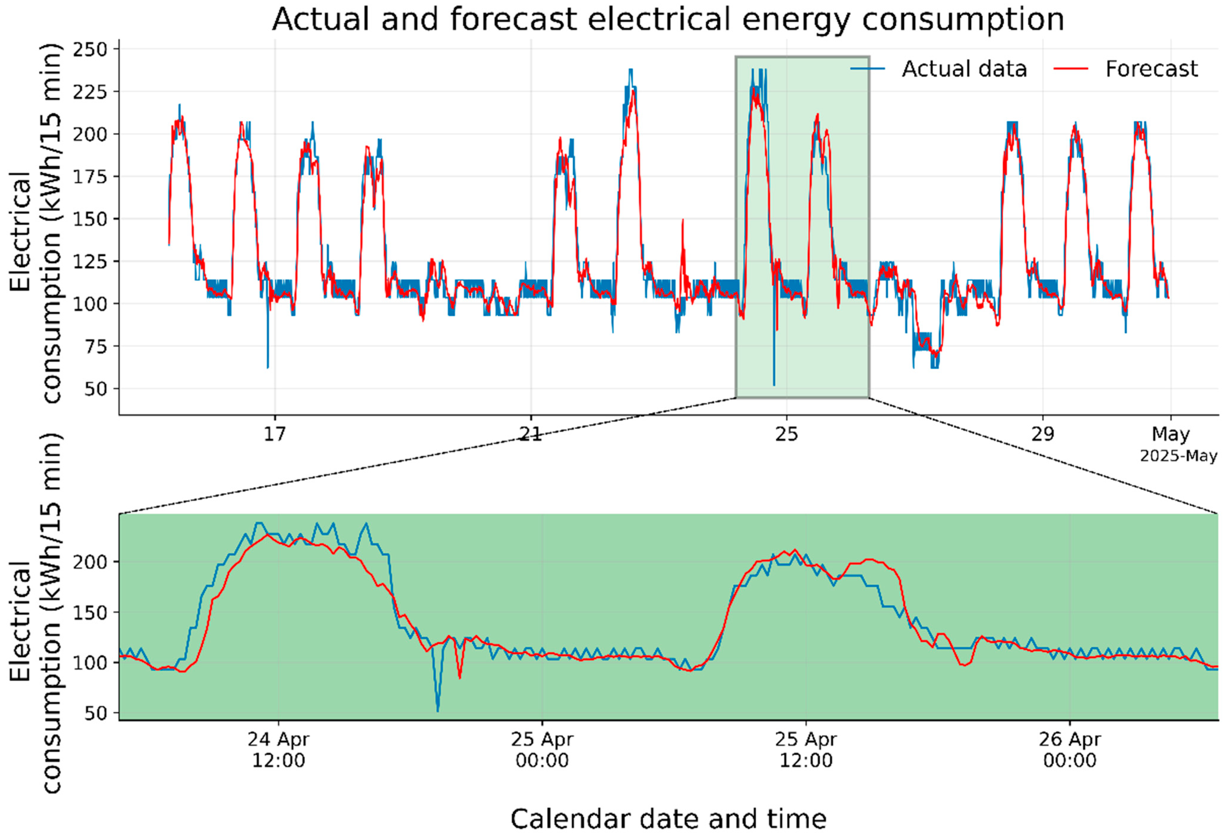
To visually examine how closely the proposed SWT + Frequency Attention + TCN model follows the actual consumption series over time, the final 1500 observations from the fourth test fold of the anchored walk-forward strategy are presented in Figure 10. This segment covers the period from 15 April 2025, at 08:15, to 30 April 2025, at 23:00. The displayed time interval consists of the chronologically final 1500 observations of the fourth test fold. The high load levels and abrupt consumption changes occurring during this period reflect the natural temporal behavior of the campus consumption profile.

Figure 10 shows that the actual and predicted consumption series follow each other closely in terms of their overall temporal patterns. The model largely captures the daily consumption variations and the main increases and decreases in load levels. Although no clear systematic delay in peak timing is observed in the zoomed section, the magnitudes of some peaks during high consumption periods are underestimated relative to the actual values. This finding is consistent with the underestimation tendency identified in Table 14 and indicates that the main limitation of the model is more closely related to the estimation of peak magnitude than to peak timing.

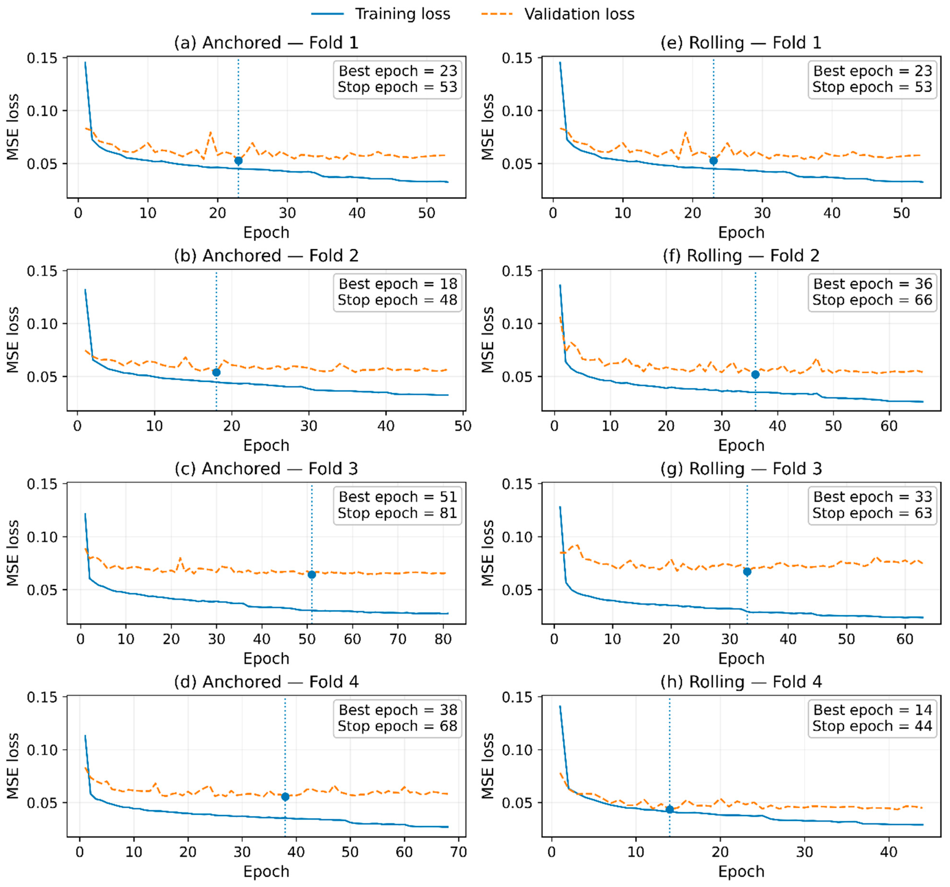
To evaluate the training behavior of the proposed model and the validation-based model selection process, the training and validation loss curves for all four folds under the anchored and rolling walk-forward strategies are presented in Figure 11. Across all folds, the training loss decreases rapidly during the initial epochs and then follows a more gradual and stable downward trend in the subsequent epochs. This indicates that the learning process of the model progresses in a stable manner without substantial instability or divergence during training.

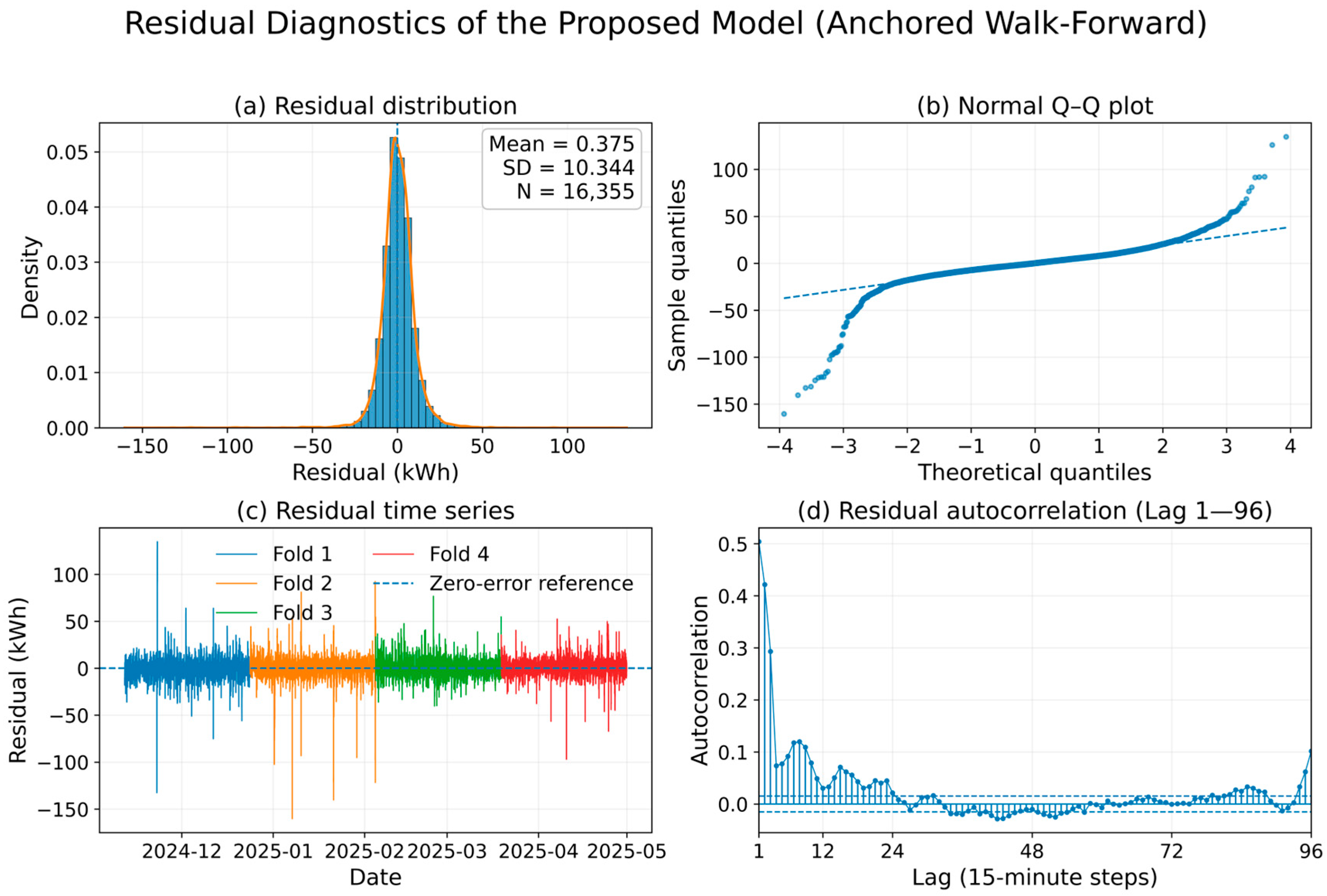
To examine the structure of the forecasting errors of the proposed model in greater detail, residual diagnostics were performed. Residual values were calculated by subtracting the predicted consumption value from the actual consumption value. Therefore, positive residual values indicate that the model underestimates consumption, whereas negative residual values indicate that it overestimates consumption. Figure 12 presents the residual distribution and normal Q-Q behavior for the 16,355 test predictions obtained under the anchored walk-forward evaluation. In addition, the residual time series across the folds and the residual autocorrelation structure up to 96 lags of 15 min each are also presented.

Under the anchored walk-forward evaluation, the mean residual was 0.375 kWh, while the standard deviation was 10.344 kWh. The overall concentration of residual values around zero indicates that the model exhibits a limited general tendency toward underestimation. However, the deviations observed particularly in the tails of the histogram and Q–Q plot indicate that the residual distribution is not normal and that relatively large forecasting errors may occur for some observations.

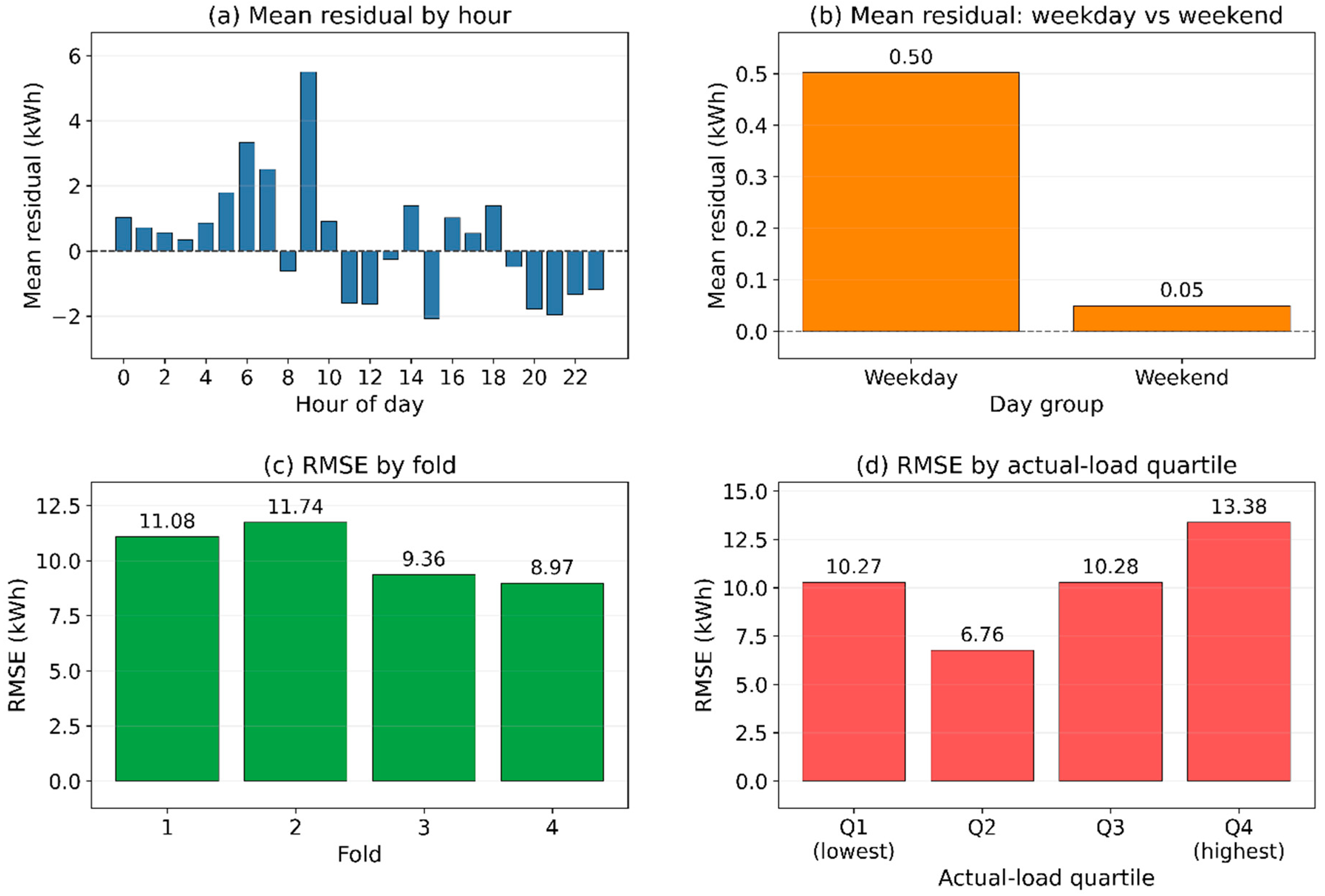
To examine the temporal and load-dependent structure of the forecasting errors, the residual values were further evaluated according to hour, weekday and weekend status, walk-forward fold, and actual consumption level. The results are presented in Figure 13.

Figure 13 shows that residual bias varies throughout the day and that the most pronounced underestimation tendency occurs around 09:00. This time corresponds to the period when classes begin at the university. The mean residual was 0.50 kWh for weekday observations and 0.05 kWh for weekend observations, indicating limited overall bias in both groups. The fold-based RMSE ranged from 8.97 to 11.74 kWh, with lower errors observed in the later folds. In terms of load level, the highest error was obtained in the Q4 group (RMSE = 13.38 kWh), indicating that high consumption levels are more challenging to forecast.

When the overall performance results, uncertainty analysis, peak load evaluation, and residual diagnostics are considered together, the proposed model provides consistent forecasting performance under different temporal evaluation conditions. However, the residual autocorrelation structure and the underestimation tendency observed at high consumption levels indicate that the model still has aspects that could be improved, particularly under peak load conditions.

4. Discussion

In this study, a hybrid forecasting model integrating SWT-based multiscale signal decomposition, a Frequency Attention mechanism, and a TCN architecture was proposed for short-term electricity consumption forecasting at the campus scale. The findings demonstrate that SWT-based multiscale representation and the Frequency Attention mechanism generally improve the forecasting performance of comparative deep learning models. SWT decomposition allows low-frequency trends and high-frequency spikes in historical electricity consumption to be represented separately. The Frequency Attention mechanism adaptively emphasizes the frequency scales that are more informative for the forecasting task. Therefore, the effectiveness of the proposed SWT + Frequency Attention + TCN architecture can be attributed to the complementary interaction among multiscale signal representation, frequency-based attention, and the temporal dependency modeling capability of the TCN. Overall, the Frequency Attention mechanism had a positive effect across different deep learning architectures. The integration of a Frequency Attention layer into the SWT-based CNN-LSTM, LSTM, BiLSTM, and TCN models generally reduced the error metrics and increased the R2 values. This finding indicates that the frequency components obtained through SWT do not contribute equally to the forecasting process. In other words, certain frequency scales contain more informative patterns for electricity consumption forecasting, and the Frequency Attention mechanism improves forecasting accuracy by assigning greater weights to these components.

Feature ablation results further showed that increasing the number of input variables did not necessarily improve forecasting accuracy. The compact configuration based on historical electricity consumption, Hour, and Day of Week outperformed the configurations that included meteorological variables. This suggests that, for the investigated campus and the one-hour-ahead forecasting task, recent consumption history and regular calendar patterns contain a substantial proportion of the predictive information.

This finding differs from that of Kim et al. [4], who analyzed the aggregated load of 23 campus buildings in Seoul using hourly data and forecast horizons ranging from 1 h to 1 day. Their study showed that weather- and calendar-related variables improved ANN-based peak load forecasting. In contrast, the present study uses 15 min electricity consumption data aggregated across 30 campus buildings and performs a direct 60 min ahead forecast in Afyonkarahisar. Meteorological variables did not provide additional improvement beyond historical consumption and calendar information. This difference may be associated with the shorter forecast horizon, finer temporal resolution, aggregation level, climatic conditions, and the strong predictive information contained in recent consumption observations. These methodological differences also limit direct numerical comparison between the two studies.

The proposed hybrid model achieved the lowest mean forecasting errors among the evaluated benchmark models under both rolling and anchored walk-forward strategies. The consistent performance across these two temporal evaluation schemes supports the temporal robustness of the proposed approach within the investigated campus dataset. The rolling walk-forward strategy evaluates model performance over moving and up-to-date temporal windows and therefore reveals its ability to adapt to changing consumption patterns. By contrast, the anchored walk-forward strategy allows the training dataset to expand over time, enabling the model to learn longer-term consumption behaviors. The strong performance of the proposed model under both validation frameworks demonstrates that the method provides a reliable forecasting structure in terms of both temporal generalization and learning stability. From the perspective of model families, the TCN-based architecture produced particularly strong results when combined with Frequency Attention. The causal convolution structure of the TCN prevents future information from leaking into the forecasting process, whereas dilated convolutions enable the model to learn both short- and long-term dependencies across previous time steps. These characteristics provide an advantage in modeling daily cycles and abrupt load variations, observed in electricity consumption data at a 15 min temporal resolution. The multiscale frequency representations obtained through SWT and the adaptive weighting performed by the Frequency Attention mechanism further support the temporal modeling capability of the TCN, thereby improving the performance of the proposed model. Short-term electricity consumption forecasting is inherently a causal time-series problem based on historical observations. Therefore, under real-time forecasting conditions in which future information is unavailable, causal architectures such as TCNs may provide a more appropriate modeling framework.

The proposed model also maintains a compact computational structure with 40,637 trainable parameters. The mean training time was approximately 174.59 s per fold under anchored evaluation and 123.86 s under rolling evaluation, while inference required approximately 0.022 and 0.020 ms per sample, respectively. These values indicate that prediction itself introduces negligible computational latency. The experimental walk-forward protocol retrained the model at approximately 43-day intervals; however, this interval should not be interpreted as an optimal operational retraining frequency. In practice, retraining should be triggered by forecast degradation or substantial changes in occupancy, building composition, or operating schedules.

The findings of this study indicate that multiscale and attention-based representations can provide an effective approach for short-term electricity consumption forecasting in complex environments such as university campuses, where heterogeneous building types, varying occupancy patterns, and temporal consumption dynamics coexist. Accurate electricity consumption forecasting may support applications such as campus energy management, load scheduling, and demand side management.

From a practical perspective, the rolling MAE and RMSE correspond to approximately 5.61% and 8.42% of the mean campus consumption, while the corresponding anchored values are approximately 5.44% and 8.16%. Relative to the maximum observed 15 min consumption, the corresponding RMSE ratios are approximately 3.11% and 3.01%. The RMSE improvement over the strongest alternative is modest in absolute terms, at 0.532 kWh under rolling evaluation and 0.575 kWh under anchored evaluation. Therefore, the present results do not establish that these differences would necessarily alter peak warning, procurement, battery scheduling, demand response, or operating cost decisions, which depend on application-specific thresholds and operating constraints. The observed tendency to underestimate peak magnitudes should also be considered in threshold-based applications.

Model performance may deteriorate when the statistical relationship between historical consumption patterns and future demand changes substantially. In a university campus environment, such structural changes may arise from major shifts in occupancy, the commissioning or closure of buildings, semester transitions, examination or vacation periods, unusual campus closures, or changes in operating schedules. Because the proposed model learns from historical consumption and calendar patterns, abrupt changes that are not represented in the training data may lead to temporary forecasting degradation until sufficient observations reflecting the new operating regime become available. Therefore, periodic model updating or retraining may be necessary when substantial changes occur in campus operation or load composition.

Limitations and Future Study

The proposed model was developed and evaluated using approximately 14 months of electricity consumption data collected from a single university campus. Consistent with several campus load forecasting studies that have evaluated predictive models using data from a single university or a limited number of campus buildings [46,47], the present study relies on site-specific measurements. Such evaluations provide valuable evidence of temporal forecasting performance under real-world operating conditions; however, the use of data from a single campus may limit the extent to which the findings can be generalized to campuses with different climatic, structural, and operational characteristics. Although the investigated dataset encompasses diverse seasonal, meteorological, and operational load conditions, the anchored and rolling walk-forward evaluations should primarily be interpreted as evidence of temporal robustness within the investigated campus record rather than as external site validation.

Second, direct occupancy measurements and detailed academic calendar indicators, such as public holidays, examination periods, semester breaks, unusual closures, and reduced occupancy periods, were not available as explicit model inputs. Consequently, changes in campus activity and user distribution are represented only indirectly through historical consumption and calendar patterns. Future studies should incorporate explicit occupancy and academic calendar information to better evaluate forecasting performance under atypical campus operating conditions.

Meteorological variables were available in the original dataset and were evaluated through feature ablation experiments. However, their inclusion did not improve forecasting accuracy for the investigated one-hour-ahead task and they were therefore excluded from the final compact model. Accordingly, the final model does not depend on the availability of meteorological observations or weather forecasts. Nevertheless, this finding may not hold for campuses or building portfolios with stronger weather-sensitive loads, and the usefulness of meteorological information should be reassessed when the framework is applied to other locations.

Finally, the present study focuses on direct one-hour-ahead forecasting. Model performance at shorter and longer forecasting horizons and under multi-step forecasting settings was not systematically evaluated. Future research should therefore validate the proposed framework using longer datasets collected from multiple campuses, building categories, and climatic regions. Such studies should investigate cross-site transferability, site-specific recalibration, and transfer-learning or domain-adaptation strategies. Incorporating explicit occupancy measurements, detailed academic calendar variables, and diverse weather-sensitive load profiles would also enable a more comprehensive assessment of the model under both regular and atypical operating conditions.