Analysis and Optimization of Electromagnetic Vibration of Permanent Magnet Synchronous Motors for Unmanned Underwater Vehicles

Abstract

Driven by the engineering requirement for high acoustic stealth of unmanned underwater vehicles (UUVs), this paper investigates the electromagnetic vibration of an 8-pole, 48-slot, surface-mounted permanent magnet synchronous motor (SPMSM) employed in the propulsion system through multi-physics coupling analysis and experimental testing. First, analytical calculations of electromagnetic force waves are performed based on the Maxwell stress tensor method and the magnetomotive force–permeance method to analyze the spatial orders, temporal orders, and sources of the harmonics. Then, a two-dimensional motor model is established using ANSYS electromagnetic field simulation software to investigate the temporal and spatial characteristics of electromagnetic force waves under both no-load and on-load conditions. Fourier decomposition is applied to obtain the amplitude-frequency characteristics, thereby verifying the correctness of the analytical results. Subsequently, three-dimensional models of the stator core and the complete stator assembly are constructed in the physical field, and their modal frequencies and mode shapes are obtained through simulation. On this basis, harmonic response analysis is conducted by applying electromagnetic force waves to the stator teeth, and vibration simulations are performed in ANSYS Workbench to acquire vibration characteristics. Vibration experiments are then carried out at multiple rotational speeds, and the experimental results are compared with the simulation results to validate the feasibility and accuracy of the finite element modeling approach. Since the measured motor vibration results are influenced not only by electromagnetic excitation forces, but also by various factors such as mechanical structure, instrument installation, and fixture conditions, while the simulation model in this paper inevitably simplifies damping, housing details, inverter control effects, and considers only the effect of radial electromagnetic forces, there exists a certain discrepancy between the simulated and measured motor vibration acceleration results. However, the main vibration trends in the low-frequency range below 800 Hz are basically consistent, particularly at the second and fourth harmonic frequencies, where the vibrations are electromagnetic vibrations caused by radial electromagnetic force waves, with relative errors between the measured and simulated values of 18% and 25%, respectively. This finite element model can be used for preliminary design evaluation of PMSMs and rapid prediction of electromagnetic vibration, providing researchers with a convenient and practical research approach and methodology. Finally, by analyzing factors that may influence motor vibration, this paper proposes design modifications to the stator structure and air-gap width, providing an optimized solution for reducing electromagnetic vibration of the permanent magnet synchronous motor and avoiding resonance.

1. Introduction

Unmanned underwater vehicles (UUVs), as critical equipment for exploring deep-sea environments and executing underwater reconnaissance and operational missions, have their propulsion system performance directly determining cruising speed, endurance, and mission reliability. Permanent magnet synchronous motors (PMSMs), by virtue of their high power density, high efficiency, wide speed range, and excellent torque dynamic response characteristics, have become the motor of choice for modern UUV propulsion systems. However, the unique operating environment of UUVs imposes extremely stringent low-vibration and low-noise requirements on their propulsion motors: on the one hand, excessive vibration and radiated noise will severely compromise the acoustic stealth of the UUV; on the other hand, propulsion motor vibration is transmitted to the hull through the shaft system, interfering with onboard precision sonar, inertial navigation systems, and optical sensors, thereby degrading detection accuracy and mission effectiveness. Therefore, conducting refined analysis and optimization of electromagnetic vibration of PMSMs for UUVs is of significant engineering value and strategic importance for enhancing the overall performance of UUVs.

Permanent magnet synchronous motors (PMSMs) are widely used in new energy vehicles, marine vessels, industrial automation equipment, aerospace actuators, and high-performance servo systems due to their advantages of high-power density, high efficiency, compact structure, and fast dynamic response [1,2,3,4]. With the increase in power density and operating speed, electromagnetic vibration and noise have gradually become important design constraints. Excessive vibration not only degrades acoustic comfort, but also accelerates bearing wear, weakens mechanical connections, and reduces long-term reliability [5].

The electromagnetic vibration of a PMSM is not determined solely by the electromagnetic field; rather, it is a coupled problem: electromagnetic force waves generated in the air-gap act on the stator teeth and yoke, while the stator assembly responds according to its own modal characteristics [6]. Radial electromagnetic force waves are usually the primary source of stator vibration. When the spatial order of such force waves coincides with a circumferential stator mode and the frequency is close to the natural frequency of that mode, the motor may enter a resonant state. Therefore, the analysis must simultaneously consider both the excitation source characteristics and the structural modal characteristics [7].

In existing studies, Lan Hua [8] derived mathematical expressions for the radial and tangential electromagnetic force waves of surface-mounted permanent magnet synchronous motors, thoroughly analyzed the harmonic characteristics of the electromagnetic force waves, and further explored the intrinsic relationship between tangential electromagnetic force waves and motor torque ripple. Li Xiaohua [9] performed theoretical derivation of electromagnetic force wave formulas for an interior permanent magnet synchronous motor used in electric vehicles and analyzed the causes of each force wave. Fang H [10] conducted electromagnetic vibration analysis of permanent magnet motors with fractional-slot concentrated windings. The study found that when the distributed electromagnetic force in the air gap is converted into concentrated forces on the stator teeth, high spatial-order electromagnetic force waves can be modulated into low-order electromagnetic force waves, thereby causing electromagnetic vibration and noise. Soresini F [11] employed viscoelastic layer materials to suppress vibration in permanent magnet synchronous motors. Reference [12] analyzed the electromagnetic vibration response of motors using the magnetic field modulation principle.

Although the studies provide valuable research directions for electromagnetic vibration control of PMSMs, specialized investigations into UUV propulsion motors remain insufficient. Existing literature predominantly focuses on automotive or industrial drive motors, whose design objectives prioritize high rotational speed and high-power density, differing significantly from the requirements of UUV propulsion motors for low-speed, high-torque, and high-reliability operation. In view of this, this paper takes an 8-pole, 48-slot permanent magnet synchronous propulsion motor for UUVs as the research object to conduct electromagnetic vibration analysis and optimization. Compared with fractional-slot configurations, this slot–pole combination produces fewer harmonic components and can effectively reduce vibration; relative to integer–slot motors with other slot–pole numbers, it offers superior electromagnetic performance. Consequently, the 8-pole, 48-slot configuration is widely adopted in propulsion motors [13,14].

First, analytical calculations of electromagnetic force waves are performed based on the Maxwell stress tensor method and the magnetomotive force–permeance method to analyze their spatial orders, temporal orders, and sources. Then, a two-dimensional motor model is established using ANSYS Maxwell 2023 R1 electromagnetic field simulation software to investigate the temporal and spatial characteristics of electromagnetic force waves under both no-load and on-load conditions. Fourier decomposition is applied to obtain the amplitude-frequency characteristics. Subsequently, three-dimensional models of the stator core and the complete stator assembly are constructed in the physical field; their modal frequencies and mode shapes are obtained through simulation to assess the resonance risk. Furthermore, the electromagnetic forces are mapped to the structural field to conduct harmonic response analysis; electromagnetic force waves are applied to the stator teeth, and vibration simulations are performed in ANSYS Workbench to acquire the vibration characteristics. Vibration experiments are then carried out at multiple rotational speeds, and the experimental results are compared with simulation results to validate the feasibility and accuracy of the finite element model analysis method. Finally, by analyzing factors that may influence motor vibration, this paper proposes design modifications to the stator structure and air-gap width, providing an optimized solution for reducing electromagnetic vibration and avoiding resonance. This paper aims to provide a theoretical basis and engineering reference for the low-vibration design of UUV propulsion motors.

2. Theoretical Analysis

2.1. Theory Electromagnetic Force Waves

Under the assumptions of negligible core saturation, eddy current losses, and rotor eccentricity, the radial and tangential magnetomotive forces (MMF) at any point in the air gap of a permanent magnet synchronous motor can be expressed as

$$\left.\begin{array}{l}{F}_r(\theta ,t)=F_{r\_\mathrm{PM}}(\theta ,t)+F_{r\_\mathrm{arm}l}(\theta ,t)\\ F_t(\theta ,t)=F_{t\_\mathrm{PM}}(\theta ,t)+F_{t\_\mathrm{arm}l}(\theta ,t)\end{array}\right\}$$

(1)

where $\theta$ is the mechanical angle between the central axis of the permanent magnet and the centerline of the adjacent stator tooth; $t$ is time; $F_{r\_\mathrm{PM}}$ and $F_{t\_\mathrm{PM}}$ are the radial and tangential magnetomotive forces generated by the permanent magnet, respectively; $F_{r\_\mathrm{arm}l}$ and $F_{t\_\mathrm{arm}l}$ are the radial and tangential harmonic magnetomotive forces generated by the armature reaction, respectively. The Fourier series expansions of the radial and tangential magnetomotive forces can be expressed as

$$\left.\begin{array}{l}{F}_{r\_\mathrm{PM}}(\theta ,t)={\displaystyle \sum _{\mu =1,3,5\cdots }{F}_{r\mu }^{\mathrm{PM}}}\cos \mu (p\theta -{\omega }_{e}t)\\ F_{t\_\mathrm{PM}}(\theta ,t)={\displaystyle \sum _{\mu =1,3,5\cdots }{F}_{t\mu }^{\mathrm{PM}}}\cos \mu (p\theta -{\omega }_{e}t)\\ F_{r\_\mathrm{arm}l}(\theta ,t)={\displaystyle \frac{3}{2}}{\displaystyle \sum _l{\displaystyle \sum _{\nu }{F}_{r\nu l}^{\mathrm{arm}}}}\cos (\nu p\theta \mp l{\omega }_{e}t)\\ F_{t\_\mathrm{arm}l}(\theta ,t)={\displaystyle \frac{3}{2}}{\displaystyle \sum _l{\displaystyle \sum _{\nu }{F}_{t\nu l}^{\mathrm{arm}}}}\cos (\nu p\theta \mp l{\omega }_{e}t)\end{array}\right\}$$

(2)

where $p$ is the number of pole pairs; ${\omega }_e$ is the electrical angular frequency; $\mu =2k_1+1$ is the harmonic order of the permanent magnet magnetomotive force, where $k_1=0,1,2,\cdots$; $l=2k_2+1$ is the order of the harmonic current, where $k_2=0,1,2,\cdots$; $\nu =6k_3+1$ is the harmonic order of the armature magnetomotive force, where $k_3=0,\pm 1,\pm 2,\cdots$; $F_{r\mu }^{\mathrm{PM}}$ and $F_{t\mu }^{\mathrm{PM}}$ are the amplitudes of the $\mu$-th radial and tangential magnetomotive forces generated by the permanent magnet, respectively; $F_{r\nu l}^{\mathrm{arm}}$ and $F_{t\nu l}^{\mathrm{arm}}$ are the amplitudes of the $\nu$-th radial and tangential magnetomotive forces produced by the $l$-th harmonic current, respectively.

Considering the effect of stator slotting, the complex relative permeance function $\lambda$ is introduced, which can be expressed as

$$\left.\begin{array}{l}\lambda ={\lambda }_a+\mathrm{j}{\lambda }_b\\ {\lambda }_a={\lambda }_0+{\displaystyle \sum _{n=1}^{\infty }{\lambda }_{an}}\cos (nZ\theta )\\ {\lambda }_b={\displaystyle \sum _{n=1}^{\infty }{\lambda }_{bn}}\sin (nZ\theta )\end{array}\right\}$$

(3)

where ${\lambda }_a$ is the real part of the complex relative permeance, characterizing the amplitude modulation component of the air-gap permeance; ${\lambda }_b$ is the imaginary part of the complex relative permeance, characterizing the phase modulation component of the air-gap permeance; ${\lambda }_0$ is the base permeance unaffected by slotting; ${\lambda }_{an}$ and ${\lambda }_{bn}$ are the coefficients of the $n$-th order expansion term of the complex relative permeance, respectively; $n$ is the $n$-th harmonic of permeance; and $Z$ is the number of stator slots.

According to the magnetomotive force–permeance method, the air-gap flux density can be expressed as

$$\left.\begin{array}{l}B(\theta ,t)=F(\theta ,t)\lambda (\theta )=B_r(\theta ,t)+{jB}_t(\theta ,t)\\ B_r(\theta ,t)=B_{r\_\mathrm{PM}}(\theta ,t)+B_{r\_\mathrm{arm}}(\theta ,t)\\ ={\displaystyle \sum _{\mu }{\displaystyle \sum _{n=0}^{\infty }{B}_{r\mu n}^{\mathrm{PM}}}}\cos \left[\left(\mu p\pm nZ\right)\theta -\mu {\omega }_{e}t\right]\\ +{\displaystyle \sum _v{\displaystyle \sum _l{\displaystyle \sum _{n=0}^{\infty }{B}_{rvnl}^{\mathrm{arm}}}}}\cos \left[\left(vp\pm nZ\right)\theta -l{\omega }_{e}t+{\phi }_l\right]\\ B_t(\theta ,t)=B_{r\_\mathrm{PM}}(\theta ,t)+B_{r\_\mathrm{arm}}(\theta ,t)\\ ={\displaystyle \sum _{\mu }{\displaystyle \sum _{n=0}^{\infty }{B}_{t\mu n}^{\mathrm{PM}}}}\sin \left[\left(\mu p\pm nZ\right)\theta -\mu {\omega }_{e}t\right]\hfill \\ +{\displaystyle \sum _v{\displaystyle \sum _l{\displaystyle \sum _{n=0}^{\infty }{B}_{tvnl}^{\mathrm{arm}}}}}\sin \left[\left(vp\pm nZ\right)\theta -l{\omega }_{e}t+{\phi }_l\right]\end{array}\right\}$$

(4)

where ${\phi }_l$ is the phase angle of the harmonic magnetic field generated by the harmonic current; $B_{r\mu n}^{\mathrm{PM}}$ and $B_{t\nu nl}^{\mathrm{arm}}$ are the amplitudes of the $\mu$-th order radial and tangential air-gap flux densities produced by the interaction of the permanent magnet magnetomotive force with the $n$-th permeance harmonic, respectively; $B_{r\nu nl}^{\mathrm{arm}}$ and $B_{t\nu nl}^{\mathrm{arm}}$ are the amplitudes of the $\nu$-th order radial and tangential air-gap flux densities produced by the interaction of the $l$-th harmonic current with the $n$-th permeance harmonic, respectively, which can be expressed as

$$\left.\begin{array}{l}{B}_{r\mu n}^{\mathrm{PM}}={\displaystyle \frac{F_{r\mu }^{\mathrm{PM}}{\lambda }_{an}\pm F_{r\mu }^{\mathrm{PM}}{\lambda }_{bn}}{2}}\\ B_{t\mu n}^{\mathrm{PM}}={\displaystyle \frac{F_{t\mu }^{\mathrm{PM}}{\lambda }_{an}\mp F_{t\mu }^{\mathrm{PM}}{\lambda }_{bn}}{2}}\\ B_{rvnl}^{\mathrm{arm}}={\displaystyle \frac{F_{r\mu l}^{\mathrm{arm}}{\lambda }_{an}\mp F_{r\mu l}^{\mathrm{arm}}{\lambda }_{bn}}{2}}\\ B_{tvnl}^{\mathrm{arm}}={\displaystyle \frac{F_{t\mu l}^{\mathrm{arm}}{\lambda }_{an}\pm F_{t\mu l}^{\mathrm{arm}}{\lambda }_{bn}}{2}}\end{array}\right\}$$

(5)

According to the Maxwell stress tensor method, the radial and tangential electromagnetic force waves can be expressed as

$$\left.\begin{array}{l}{\sigma }_r={\displaystyle \frac{1}{2{\mu }_0}}\left(B_r^2-B_{\tau }^2\right)\\ {\sigma }_t={\displaystyle \frac{1}{{\mu }_0}}{B}_r{B}_{\tau }\end{array}\right\}$$

(6)

where ${\sigma }_r$ and ${\sigma }_t$ are the radial and tangential electromagnetic force densities, respectively; ${\mu }_0=4\pi \times {10}^{-7} \mathrm{H}/\mathrm{m}$ is the permeability of free space. In PMSM surface force analysis, the tangential magnetic flux density component is typically much smaller than the radial component. Therefore, to simplify the calculation, the $B_{\tau }^2$ term in the equation is neglected in subsequent analyses of this paper [8]. This simplification does not affect the analysis of harmonic sources, spatial orders, and temporal frequencies. The radial electromagnetic force density can then be expressed as

$${\sigma }_r={\displaystyle \frac{1}{2{\mu }_0}}{B}_r^2={\displaystyle \frac{{\left(B_{r\_\mathrm{PM}}+B_{r\_arm}\right)}^2}{2{\mu }_0}}={\displaystyle \frac{B_{r\_\mathrm{PM}}^2}{2{\mu }_0}}+{\displaystyle \frac{B_{r\_\mathrm{PM}}{B}_{r\_arm}}{{\mu }_0}}+{\displaystyle \frac{B_{r\_arm}^2}{2{\mu }_0}}$$

(7)

Similarly, the tangential electromagnetic force density can be expressed as

$$\begin{array}{l}{\sigma }_t={\displaystyle \frac{\left(B_{r\_\mathrm{PM}}+B_{r\_\mathrm{arm}}\right)\left(B_{t\_\mathrm{PM}}+B_{t\_\mathrm{arm}}\right)}{2{\mu }_0}}\\ ={\displaystyle \frac{B_{r\_\mathrm{PM}}{B}_{t\_\mathrm{PM}}}{2{\mu }_0}}+{\displaystyle \frac{B_{r\_\mathrm{PM}}{B}_{t\_\mathrm{arm}}+B_{t\_\mathrm{PM}}{B}_{r\_\mathrm{arm}}}{2{\mu }_0}}+{\displaystyle \frac{B_{r\_\mathrm{arm}}{B}_{t\_\mathrm{arm}}}{2{\mu }_0}}\end{array}$$

(8)

During no-load operation of the PMSM, the armature current is zero, and the air-gap magnetic field is produced by the interaction between the permanent magnet magnetomotive force and the airgap permeance. Since the permanent magnet magnetomotive force harmonics are of odd order, the temporal orders of the no-load electromagnetic force waves are even, meaning that the force wave frequencies are typically even multiples of the electrical frequency. In the spatial domain, the zeroth-order component corresponds to the pulsating force wave, while the minimum non-zero spatial order is determined by the greatest common divisor of $2p$ and $Z$.

For the PMSM investigated in this paper, $p=4$ and $Z=48$; therefore, $r_{\min }=GCD(8,48)=8$. All other non-zero spatial force wave orders are integer multiples of 8. This result directly explains why the eighth order and its associated harmonics must be emphasized in electromagnetic vibration assessment.

Under load operation, armature reaction introduces additional magnetomotive-force harmonics. The radial and tangential force waves then simultaneously include the interactions among permanent-magnet magnetomotive force, armature-reaction magnetomotive force, and stator permeance. Even if the stator slotting effect is neglected, the interaction between the permanent magnet and armature magnetic fields can still excite force-wave components with the same basic spatial order [15]. Consequently, load operation does not change the basic pole-slot order relationship, but it can change the amplitude distribution of the force harmonics.

It can be seen from Equations (7) and (8) that electromagnetic force waves result from the interaction between two magnetic fields. In this paper, ${\mu }_1$, $v_1$, $n_1$, and $l_1$ are defined as the harmonic orders of the permanent magnet, armature, permeance, and current components in the former magnetic field, respectively, while ${\mu }_2$, $v_2$, $n_2$, and $l_2$ are the harmonic orders of the corresponding components in the latter magnetic field. Analyzing the spatial and temporal characteristics of electromagnetic force waves is of crucial significance for investigating electromagnetic vibration. By substituting the results of Equation (4) into Equations (7) and (8), the specific expressions for the radial and tangential electromagnetic force waves can be obtained, along with the harmonic sources and spatial–temporal orders of the electromagnetic force waves under load conditions, as listed in

Table 1. Harmonic sources and orders of electromagnetic force waves under load.

Direction	Source	Space Order	Time Order
Radial	PM MMF and stator permeance	$({\mu }_1\pm {\mu }_2)p+(n_1\pm n_2)Z$	$({\mu }_1\pm {\mu }_2)$
Radial	PM MMF, armature MMF, and permeance	$({\mu }_1\pm {\nu }_2)p+(n_1\pm n_2)Z$	$({\mu }_1\pm l_2)$
Radial	Armature MMF and stator permeance	$(v_1\pm v_2)p+(n_1\pm n_2)Z$	$(l_1\pm l_2)$
Tangential	Same as radial	Same as radial	Same as radial

.

2.2. Modal Analysis Theory

The structural modes of a motor are inherent properties that are independent of external excitations. According to Hamilton’s principle, by treating the motor stator as a multi-degree-of-freedom forced vibration system, the vibration equation of the permanent magnet synchronous motor can be expressed as

$$M\ddot{x}+C\dot{x}+Kx=F_{\mathrm{r}}(t)$$

(9)

where ${\mathit{F}}_{\mathbf{r}}\left(t\right)$ is the radial electromagnetic force vector; $\mathit{M}$ is the mass matrix of the motor; $\mathit{C}$ is the damping matrix; $\mathit{K}$ is the stiffness matrix; $\mathit{x}$ is the displacement vector; $\dot{\mathit{x}}$ is the velocity vector; and $\ddot{\mathit{x}}$ is the acceleration vector.

For the vibration of the motor, it can be regarded as a free simple harmonic motion, with the vibration displacement varying sinusoidally with time. The analysis of the motor modes is thus transformed into solving the vibration differential equation, when calculating the modal natural frequencies of a system under free vibration, no external force is applied; therefore, the system damping is neglected and the solution can be written as

$$M\ddot{x}+Kx=F_{\mathrm{r}}(t)$$

(10)

The solution to this differential equation takes the form

$$x\left(t\right)=\phi e^{j\omega t}$$

(11)

where $\phi$ is the modal vector and $e^{\omega }$ is the modal natural frequency. Substituting Equation (11) into Equation (10) and solving yields

$$\left(\begin{array}{c}K-{\omega }^{2}M\end{array}\right)\phi e^{j\omega t}=0$$

(12)

When $\left|K-{\omega }^{2}M\right|=0$, the differential equation admits a non-zero solution. By solving Equation (12), the eigenvalue ${\omega }_i^2$ is obtained, and the corresponding eigenvector is the mode shape, whose natural frequency is $f_i={\displaystyle \frac{w_i}{2\pi }}$.

Because electromagnetic force waves mainly act in the radial direction on the stator inner surface, circumferential modes are more relevant than purely axial modes for the present vibration problem.

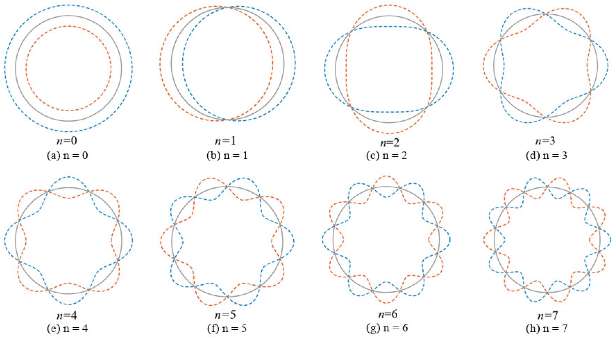
For mechanism interpretation, the stator can also be simplified as a single-ring model. In this model, the stator yoke is regarded as an equivalent cylindrical ring of uniform thickness, and the teeth and windings are converted into additional mass. The zero-order breathing mode corresponds to uniform radial expansion and contraction. For higher circumferential orders, the number of nodal diameters increases with modal order. Higher-order modes usually have higher natural frequencies and denser local deformation, while low-order modes are more likely to couple with low-order electromagnetic force waves. The circumferential mode shapes of the equivalent single-ring stator model are shown in Figure 1. In the figure, the black solid line represents the initial position of the stator, while the red and blue dashed lines represent the states at maximum stator deformation, respectively.

3. Finite-Element Electromagnetic Model

3.1. Model Establishment

In this study, the ANSYS Maxwell 2D 2023 R1 software is employed to establish a transient electromagnetic field finite element model, and the magnetic vector potential method is adopted as the solver to achieve accurate electromagnetic field computation. By importing the parametric geometric model of the stator and rotor, setting the material properties and the moving domain, and applying periodic boundary conditions along with harmonic current excitation, the air-gap magnetic field is solved, and its distribution characteristics are obtained. This provides high-precision input field data for the analysis of electromagnetic force waves.

For the electromagnetic field simulation analysis of the PMSM, a parametric model must first be constructed. The basic performance parameters of the motor model built in this paper are listed in Table 2, and the material models in the ANSYS material library for the stator core, rotor core, permanent magnets, armature windings, etc., are listed in Table 3, ensuring that the material properties selected from the ANSYS material library are similar or identical to those of the actual motor materials.

Table 2. Basic parameters of the PMSM model.

Parameter	Value	Parameter	Value
Stator outer diameter	155 mm	Stack length	110 mm
Stator inner diameter	105 mm	Air-gap length	1 mm
Rated power	1 kW	Rated speed	3000 rpm
Pole pairs	4	Stator slots	48
Pole-arc coefficient	0.7	Slot type	Pear-shaped slot

Table 2. Basic parameters of the PMSM model.

Parameter	Value	Parameter	Value
Stator outer diameter	155 mm	Stack length	110 mm
Stator inner diameter	105 mm	Air-gap length	1 mm
Rated power	1 kW	Rated speed	3000 rpm
Pole pairs	4	Stator slots	48
Pole-arc coefficient	0.7	Slot type	Pear-shaped slot

Table 3. Material assignment of the finite-element model.

Component	Material	Relative Permeability
Stator core	DW315_50_2DSF0.950	the B-H curve is shown in Figure 2
Rotor core	DW315_50_2DSF0.950	the same as the stator core.
Permanent magnet	XG196/96_2DSF1.000	1.0
Armature winding	Copper	0.999991

Table 3. Material assignment of the finite-element model.

Component	Material	Relative Permeability
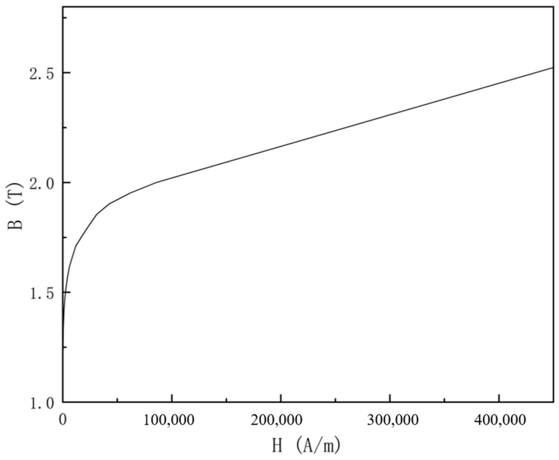
Stator core	DW315_50_2DSF0.950	the B-H curve is shown in Figure 2
Rotor core	DW315_50_2DSF0.950	the same as the stator core.
Permanent magnet	XG196/96_2DSF1.000	1.0
Armature winding	Copper	0.999991

Figure 2. B-H curve of the iron core material.

Figure 2. B-H curve of the iron core material.

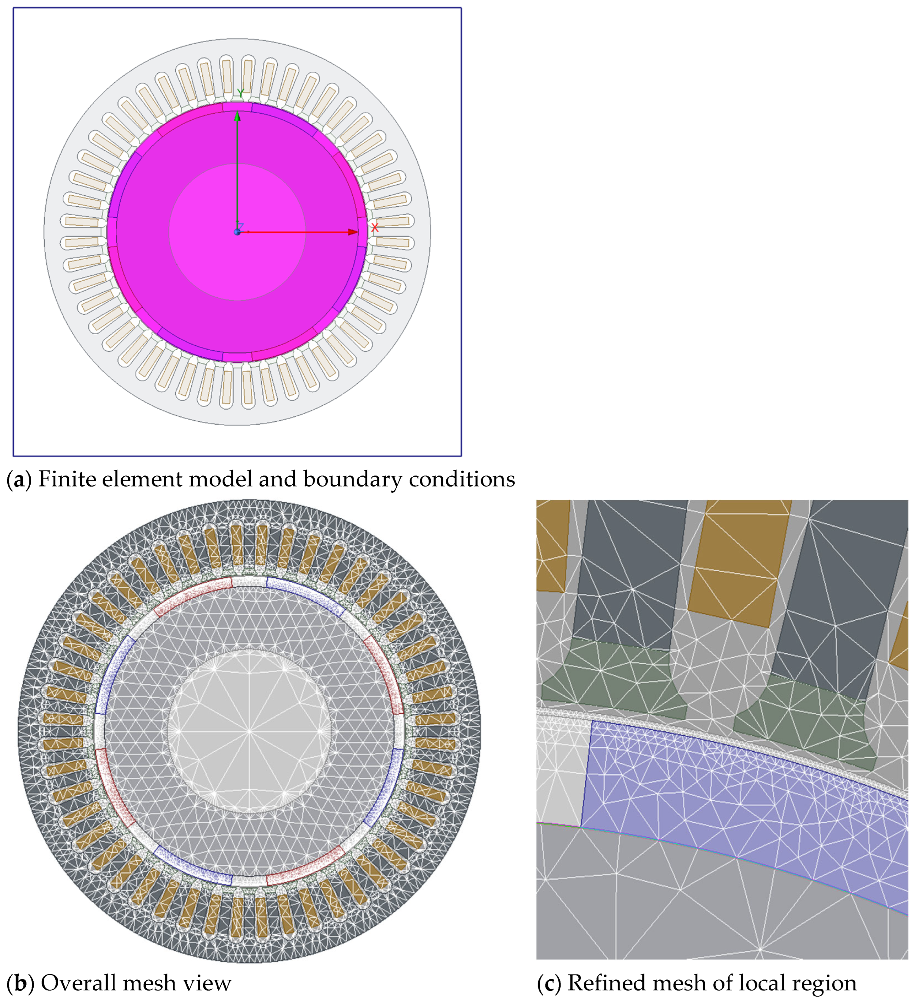
As shown in Figure 3a, the blue border encompassing the entire motor model is defined as the boundary of the computational domain, while the pink circular region containing the rotor core, permanent magnets, and air gap is designated as the moving region. The Surface Approximation method is first adopted to perform a coarse meshing of the boundary domain of the motor, with the option set to “Middle”. Subsequently, the Inside Selection method is used to apply Length-Based meshing to the stator and rotor cores, permanent magnets, armature windings, and the air gap, with the maximum element size set to 35.96 mm. Since the air-gap magnetic field serves as the transmission path of the electromagnetic force waves, and the electromagnetic force waves act on the stator teeth to induce electromagnetic vibration, a fine meshing is required for both the air-gap field and the stator teeth. The maximum element size for these regions is set to 0.25 mm, the PMSM is discretized with multi-layered meshes of varying sizes, with the air-gap region being refined into five layers. Consequently, this level of mesh refinement is sufficient to satisfy the analysis requirements of this paper, as shown in Figure 3b,c.

3.2. Magnetic Flux Density Distribution

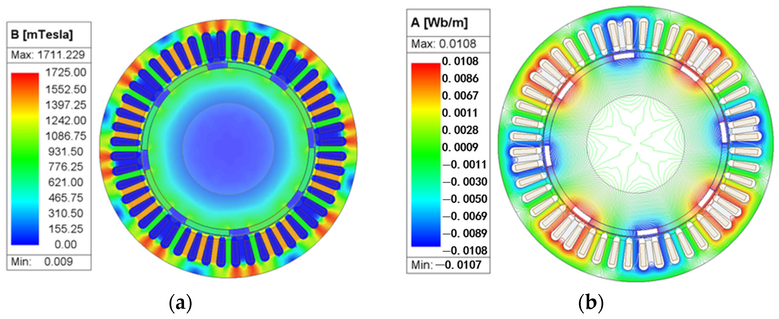
Under no-load conditions, the magnetic field is generated solely by the magnetomotive force of the permanent magnets. At this point, the excitation current is set to zero in the Excitations menu of the Maxwell 2D interface, the rotational speed is set to 3000 rpm, the simulation duration ranges from 0 to 0.1 s, the time step is set to 5 × 10⁻⁵ s, the period is half an electrical period, and the number of sampling windows is 1. A point in the air gap is selected with coordinates (52, 0); using this coordinate as the radius and (0, 0) as the center, an air-gap line is drawn. Solving the model yields the air-gap magnetic field strength along this air-gap line as well as the magnetic field distribution of the entire motor. Figure 4 shows the magnetic flux density cloud map and magnetic flux line distribution of the PMSM under no-load operation at the instant of 0.05 s.

4. Electromagnetic Force-Wave Analysis

4.1. No-Load Force-Wave Characteristics

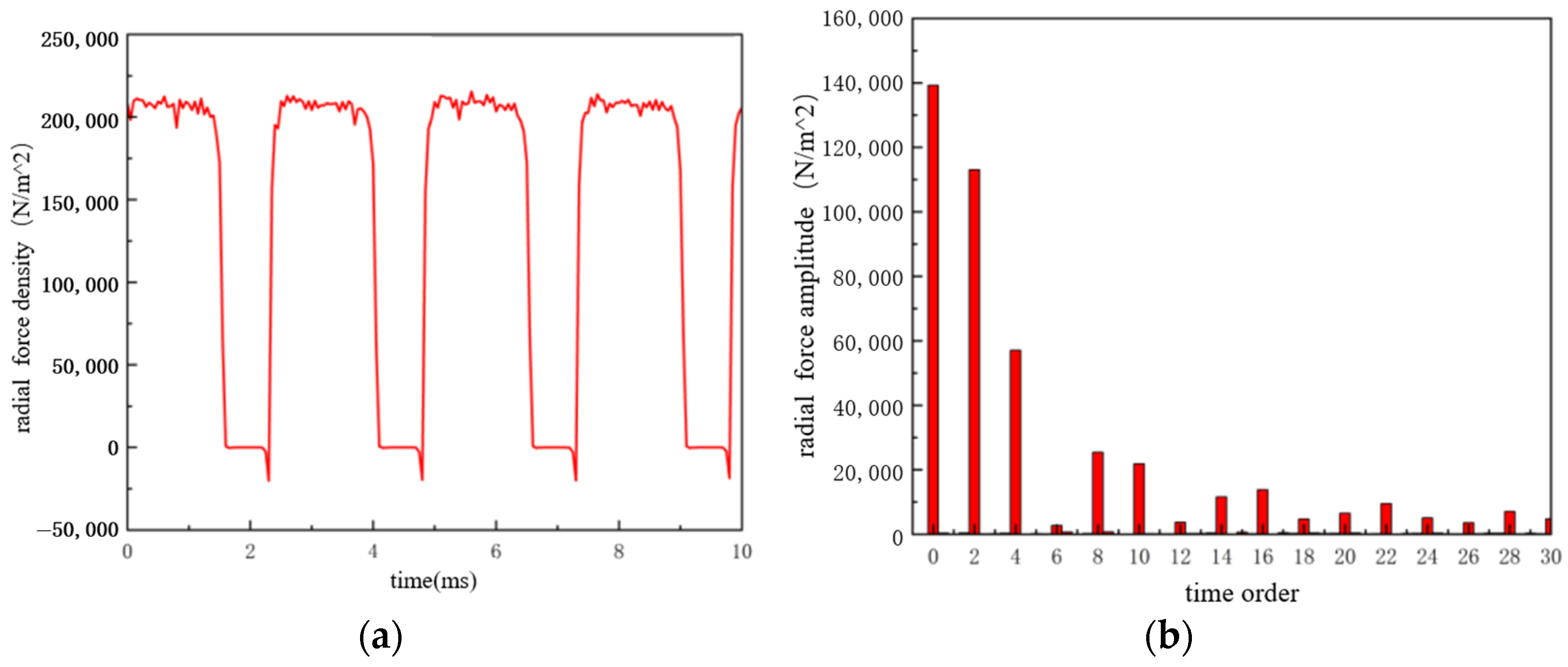
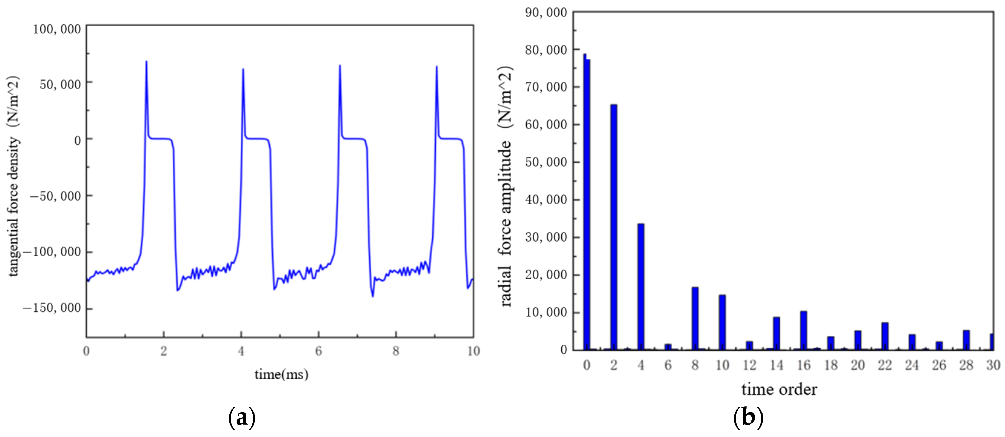
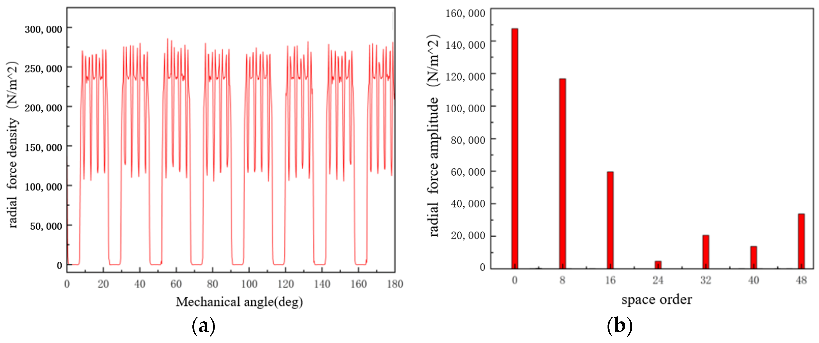
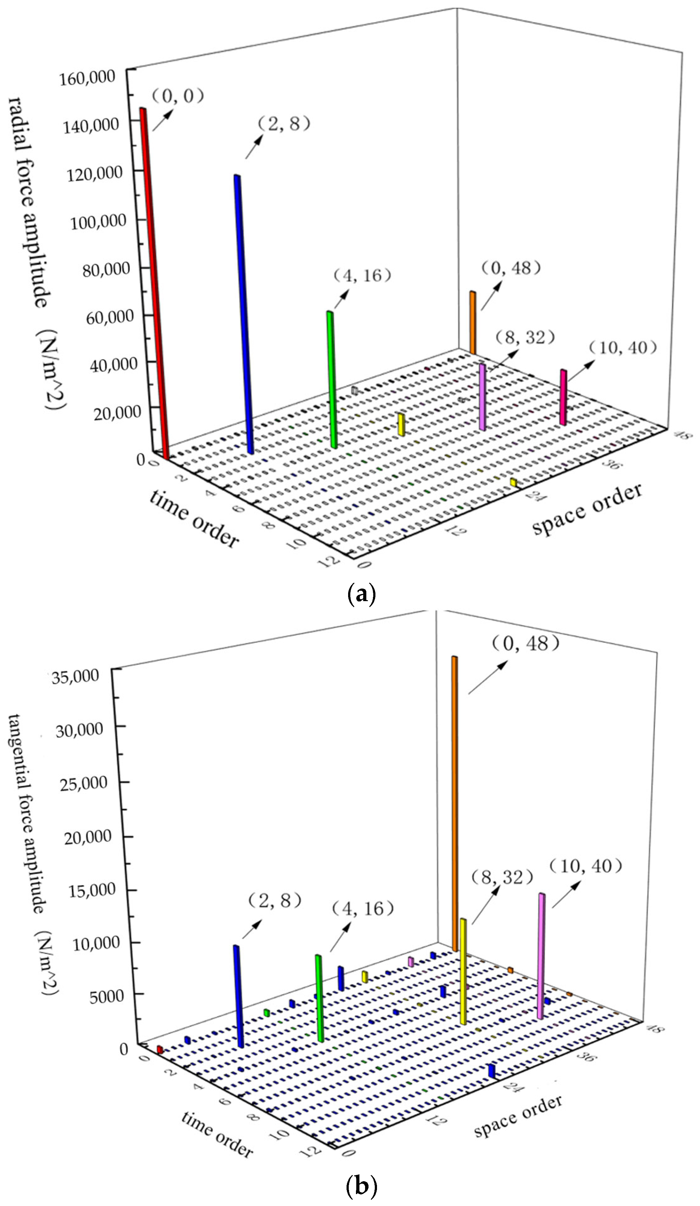
The motor speed, simulation duration, time step, number of periods, and number of sampling windows remain consistent with those in the previous section, and this setting is applied in all subsequent simulations. The current excitation is set to zero, the air-gap line is selected, and the calculation expressions for radial and tangential electromagnetic forces are entered into the Maxwell field calculator. The spatial and temporal characteristics of the no-load electromagnetic force density are then analyzed. The spatial distributions of the no-load radial and tangential electromagnetic force densities are shown in Figure 5a and Figure 6a, respectively, while the temporal distributions are shown in Figure 7a and Figure 8a. To facilitate the investigation of the sources of force waves causing electromagnetic vibration, the time-domain waveforms of the electromagnetic force waves are usually transformed into the frequency domain for analysis. According to the spatial order normalization condition and temporal frequency normalization condition [16], FFT operations are performed on 500 spatial sampling points and 100 temporal sampling points of each dataset using the built-in FFT analysis function of ANSYS. The spatial FFT spectra of the no-load radial and tangential electromagnetic force densities are shown in Figure 5b and Figure 6b, respectively, while the temporal FFT spectra are shown in Figure 7b and Figure 8b.

Since the simulation time ranges from 0 to 0.01 s, i.e., half an electrical period, the mechanical angle in Figure 5a and Figure 6a spans 0–180°. It can be observed from Figure 5, Figure 6, Figure 7 and Figure 8 that the electromagnetic force waves exhibit periodic distribution along the mechanical angle. The amplitude of the radial electromagnetic force density is much larger than that of the tangential electromagnetic force density, which validates the inference that radial electromagnetic force is the primary source of motor electromagnetic vibration. From the FFT results, the harmonic orders of the radial and tangential electromagnetic forces are identical, because they are generated by the interaction of the same magnetic field and differ only in amplitude and phase. The spatial FFT results show that the main orders of the electromagnetic force waves appear at 0, 8, 16, 32, 40, and 48. Among them, the zeroth-order component is a pulsating component, the eighth-order component is the minimum non-zero component, and all other spatial orders are integer multiples of the minimum non-zero spatial order 8, which is consistent with the conclusion derived in Section 2. The force with a spatial order of 0 is a special case and requires separate discussion: if its temporal order is also 0, the resulting force is a static force acting on the stator and rotor without causing motor vibration; if its temporal order is non-zero, the resulting force manifests as a pulsating standing wave that does not rotate in space. The temporal FFT results indicate that the temporal orders of the no-load radial electromagnetic force waves are all even, which also agrees with the conclusion obtained in Section 2.

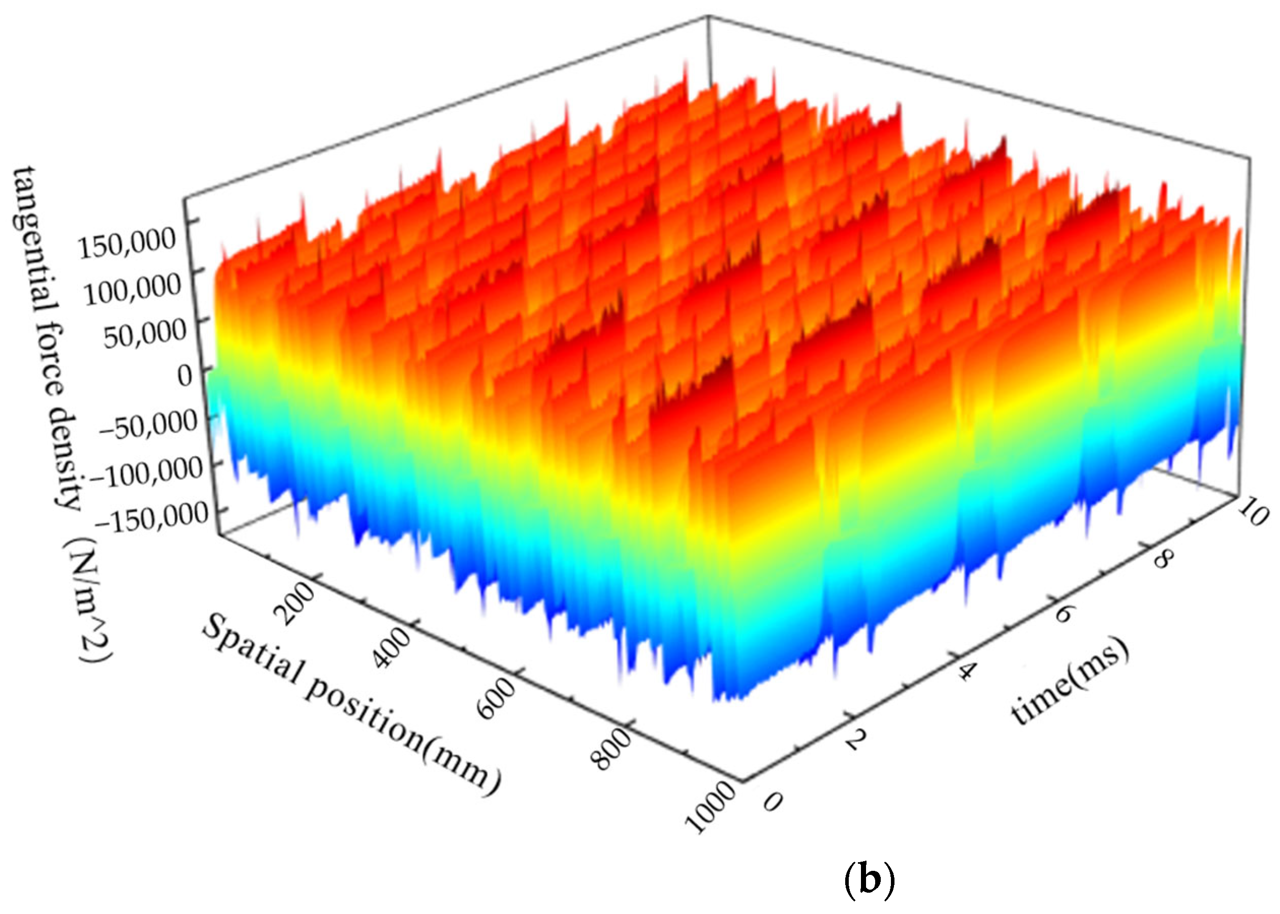
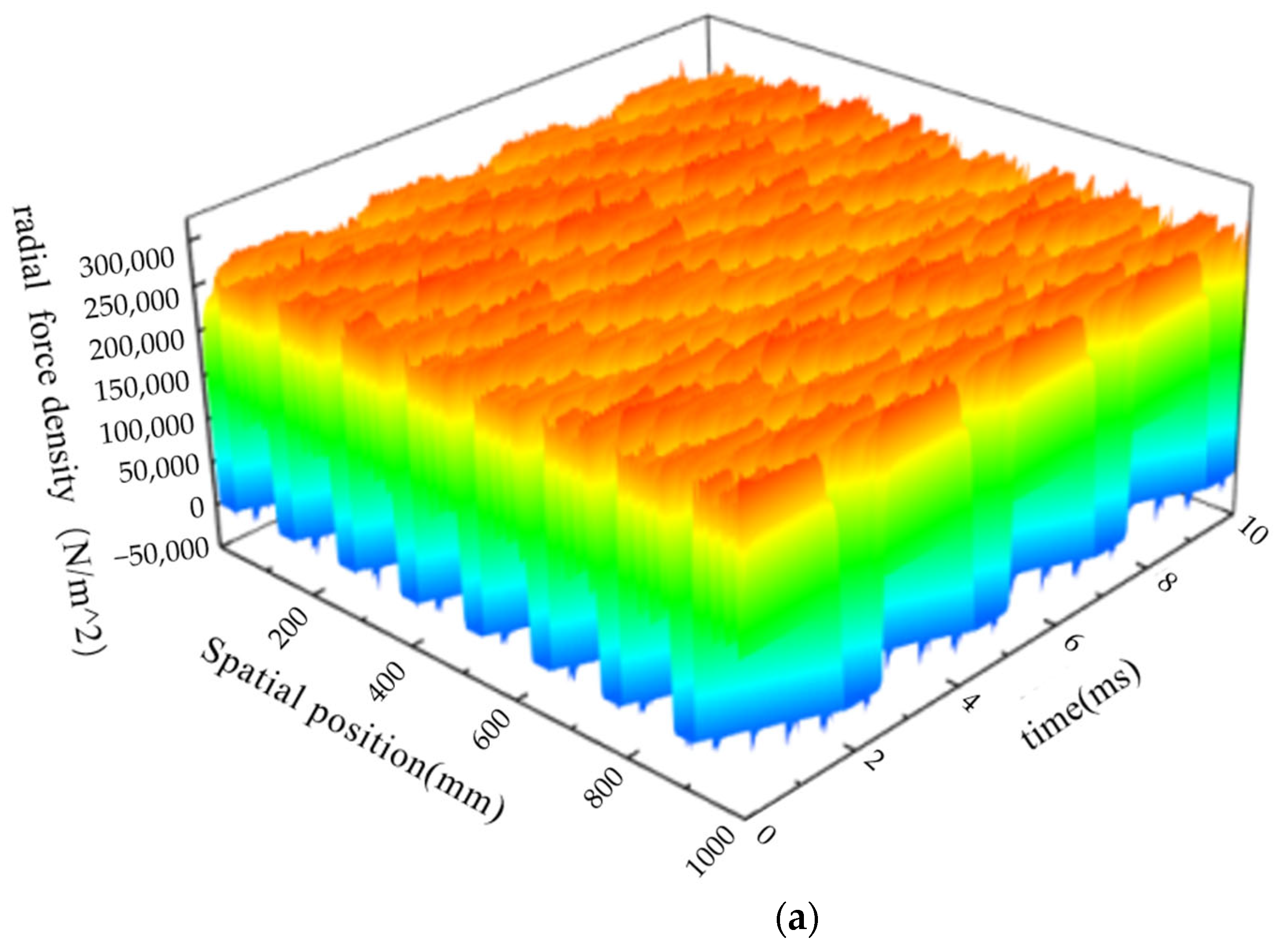
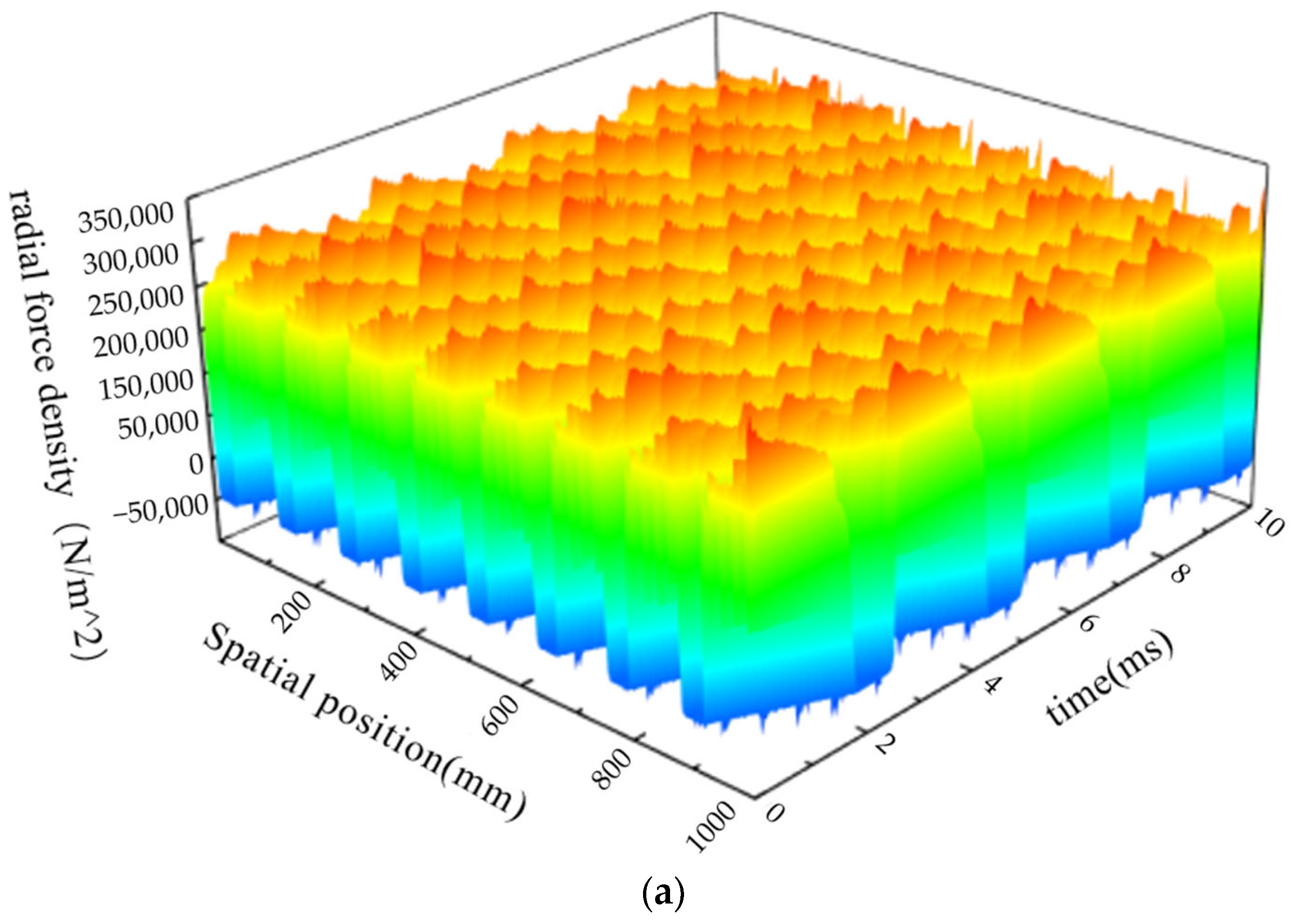
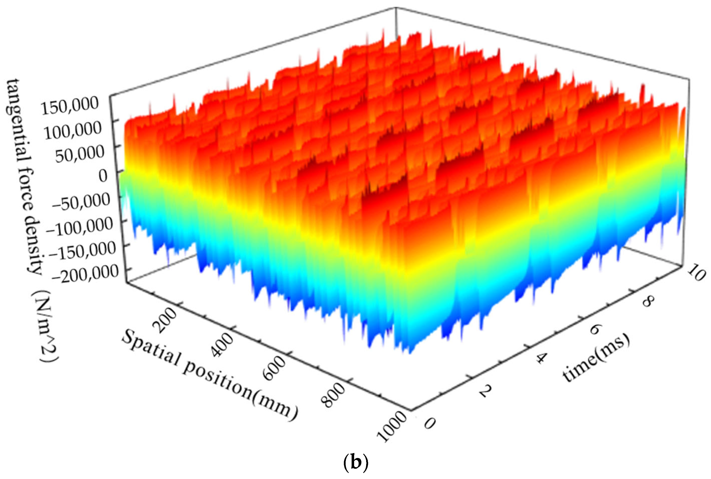
To better illustrate the spatial–temporal characteristics of the electromagnetic force waves, the spatial–temporal waveforms of the no-load radial and tangential electromagnetic force waves and their two-dimensional Fourier decomposition maps are plotted in Figure 9 and Figure 10, respectively. In Figure 9, the color scale indicates the magnitude of electromagnetic force density, with red denoting higher values and blue denoting lower values.

It can be seen from Figure 10a that the radial electromagnetic force with a spatial order of 0 and a temporal order of 0 has the largest amplitude. However, the electromagnetic force at the zeroth harmonic (zero-frequency) is a static electromagnetic force that does not excite motor vibration; therefore, the zeroth harmonic force is not considered in the vibration analysis. According to reference [17], when considering only the circumferential modes of the stator core, the vibration displacement of the stator core is inversely proportional to the fourth power of the spatial order of the force wave. Consequently, radial force waves with lower spatial orders are more likely to induce vibration. Denoting the spatial order as $r$ and the temporal order as $f$, and neglecting high-order electromagnetic force waves, the electromagnetic force has the largest amplitude and should be the focus when analyzing the no-load motor vibration. Two-dimensional Fourier analysis further confirms that identical families of orders exist in both the radial and tangential force waves. From an engineering perspective, the pole–slot combination determines the possible spatial orders, while the current, saturation, slot geometry, and operating conditions mainly alter the amplitude distribution. Therefore, both force-wave order avoidance and modal frequency avoidance should be considered simultaneously. In order to prevent the stator natural frequency from approaching or coinciding with the force wave frequency of the radial electromagnetic force—thereby causing resonance and increasing vibration and noise—the radial electromagnetic force density responsible for motor electromagnetic vibration and noise is investigated.

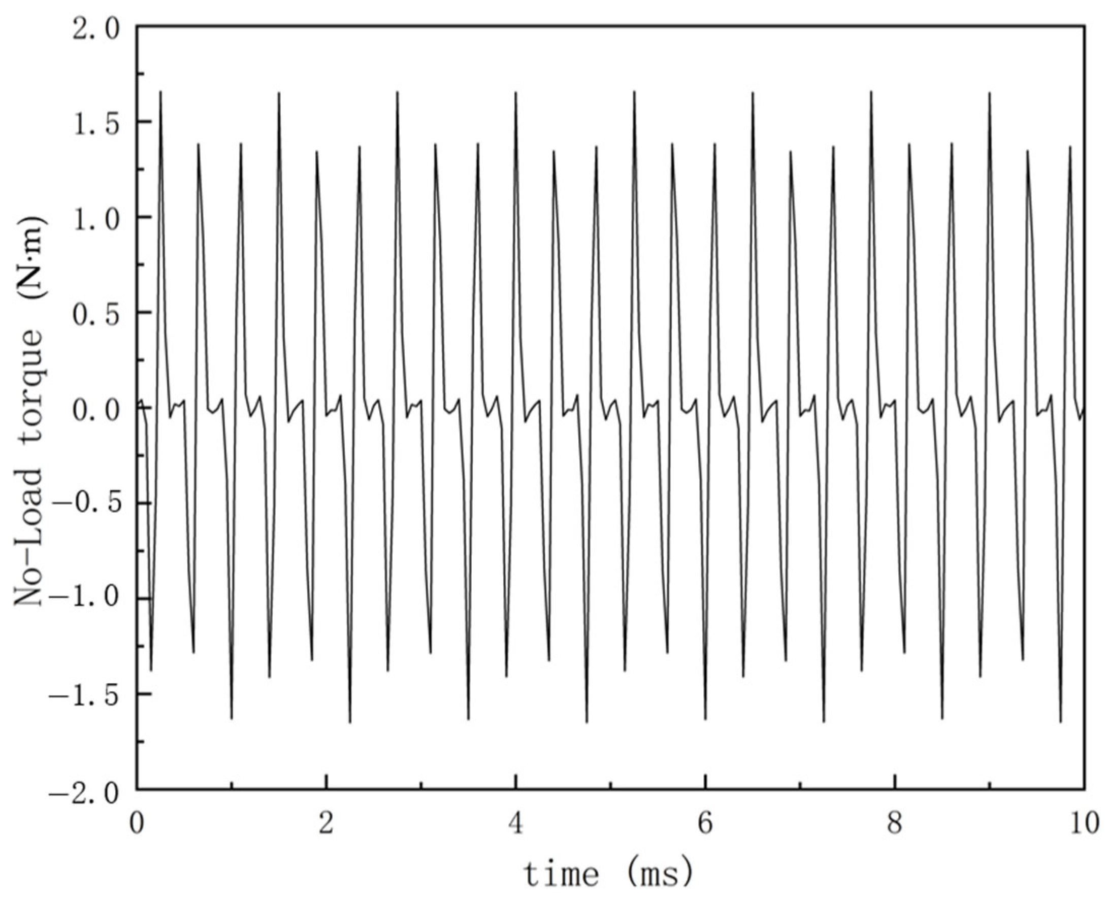
The no-load output torque is shown in Figure 11.

According to the Maxwell stress tensor equation, the output torque can be obtained by integrating the tangential electromagnetic force along the circumferential direction:

$$T=L{r}^2{\displaystyle {\int }_0^{2\pi }{\sigma }_{\mathrm{t}}}\mathrm{d}\theta$$

(13)

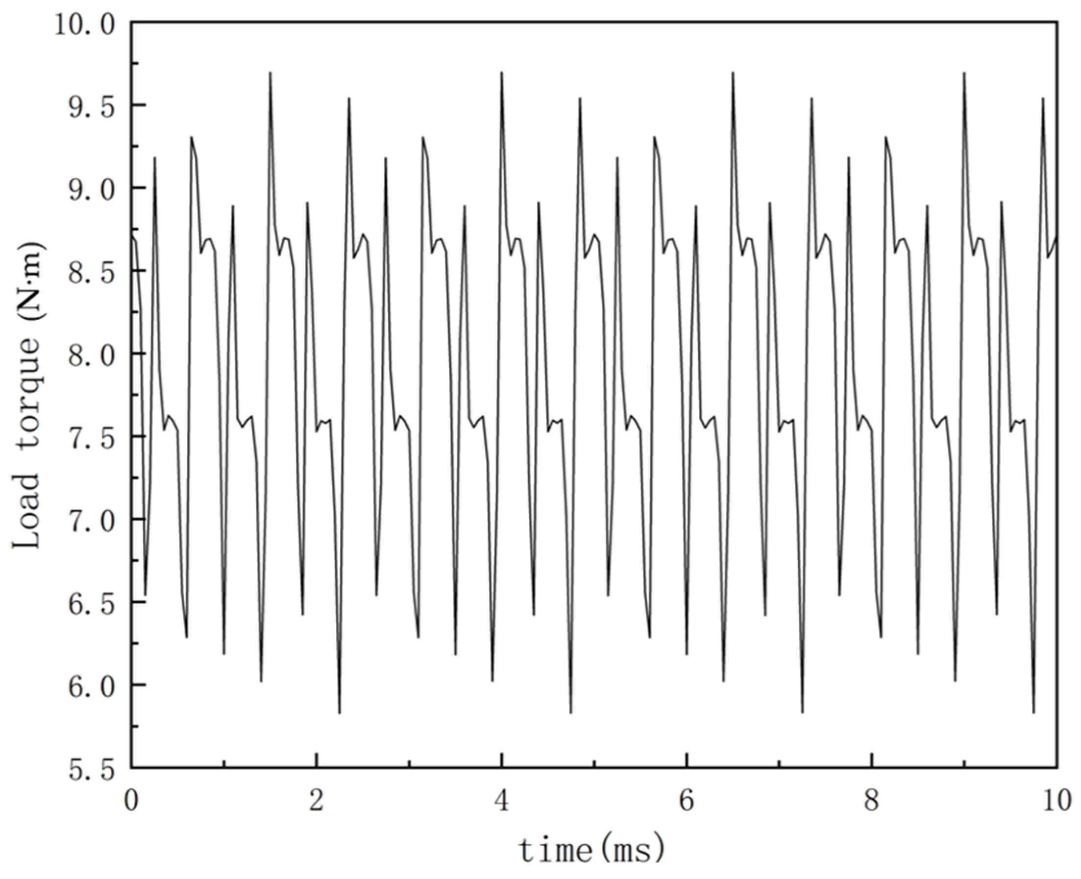
where $L$ is the stator core length and $r$ is the integration radius. It should be noted that the torque ripple of the motor is not equivalent to the tangential electromagnetic force; the torque ripple originates solely from the spatial zeroth-order tangential electromagnetic force [18]. Torque ripple contributes relatively little to the electromagnetic noise of the drive motor itself, but it can induce vibration in the entire electric propulsion system. When the frequency of the torque harmonic is close to the natural frequency of the system, resonance will occur [19]. Therefore, the tangential component is more closely related to torque ripple, while the radial component is the primary source of structural vibration. For vibration analysis, priority should be given to the low-order radial components, as they are more likely to couple with low-order circumferential modes of the stator.

4.2. Load Force-Wave Characteristics

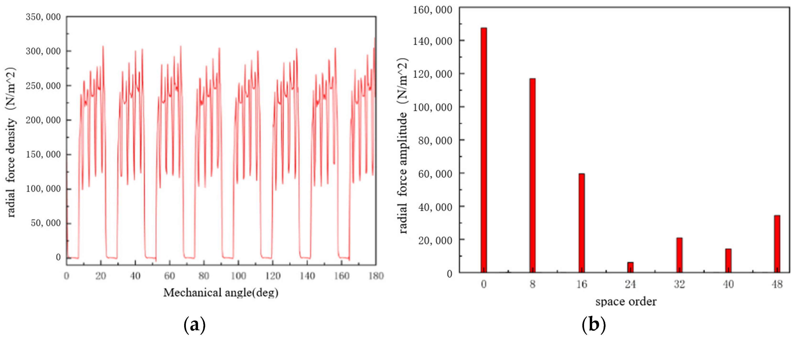
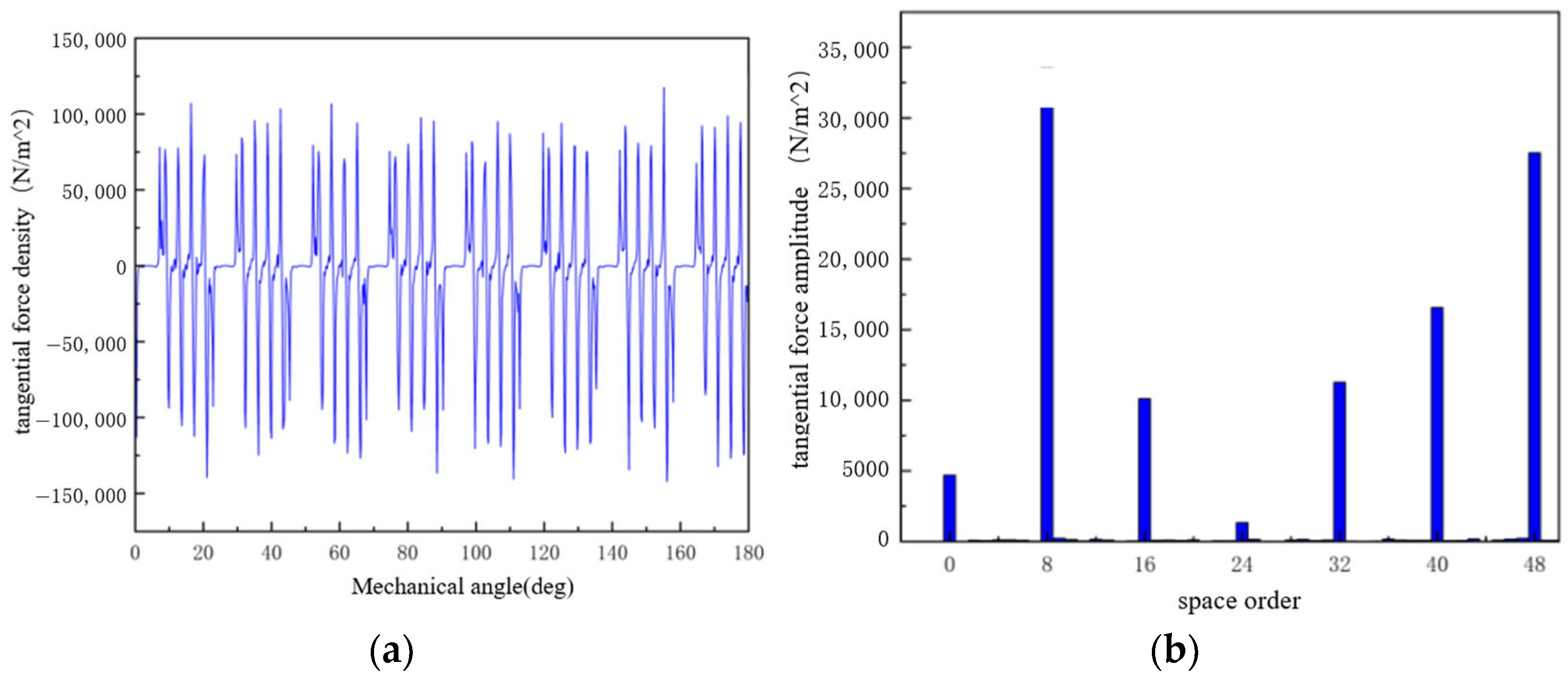
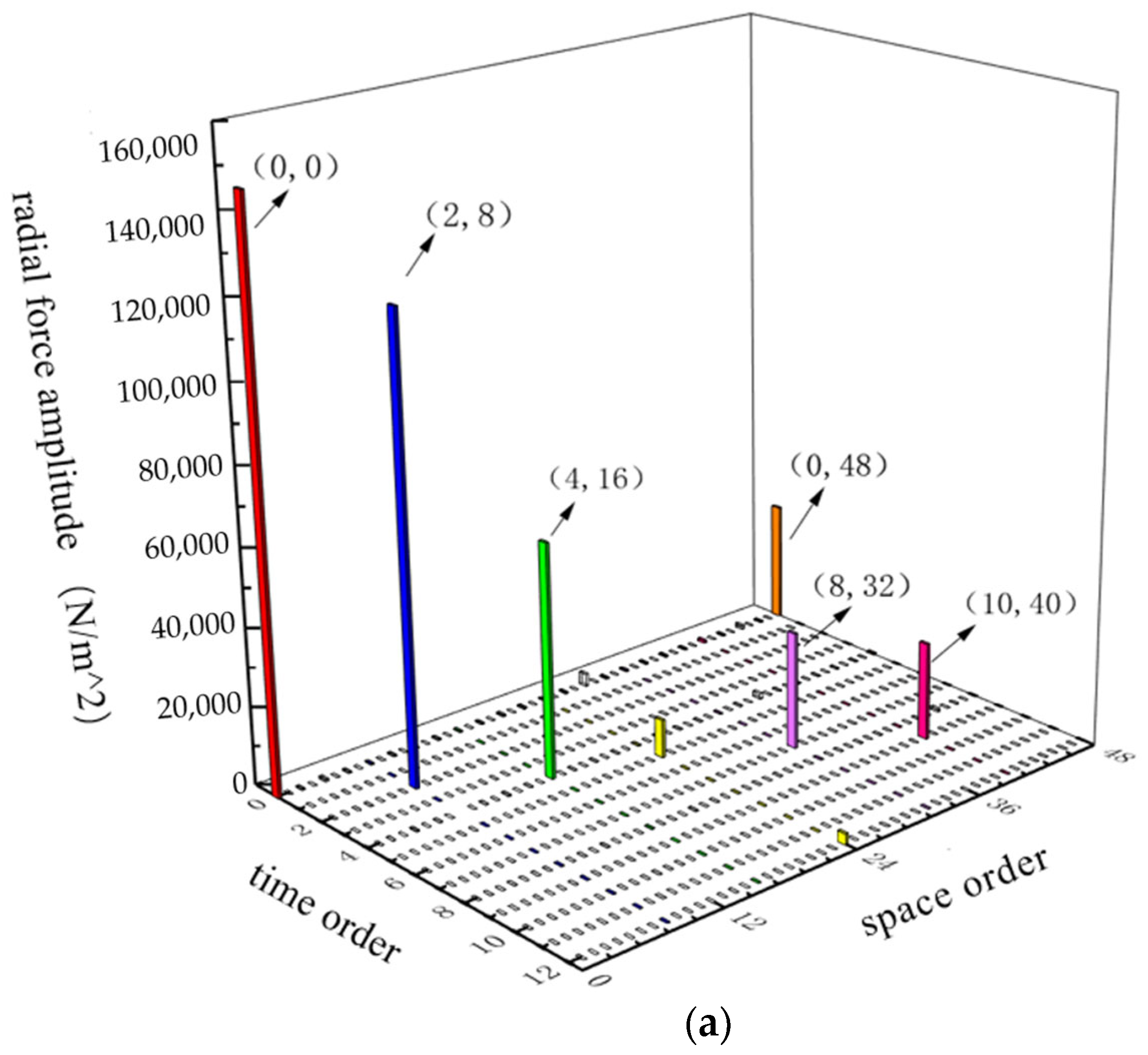
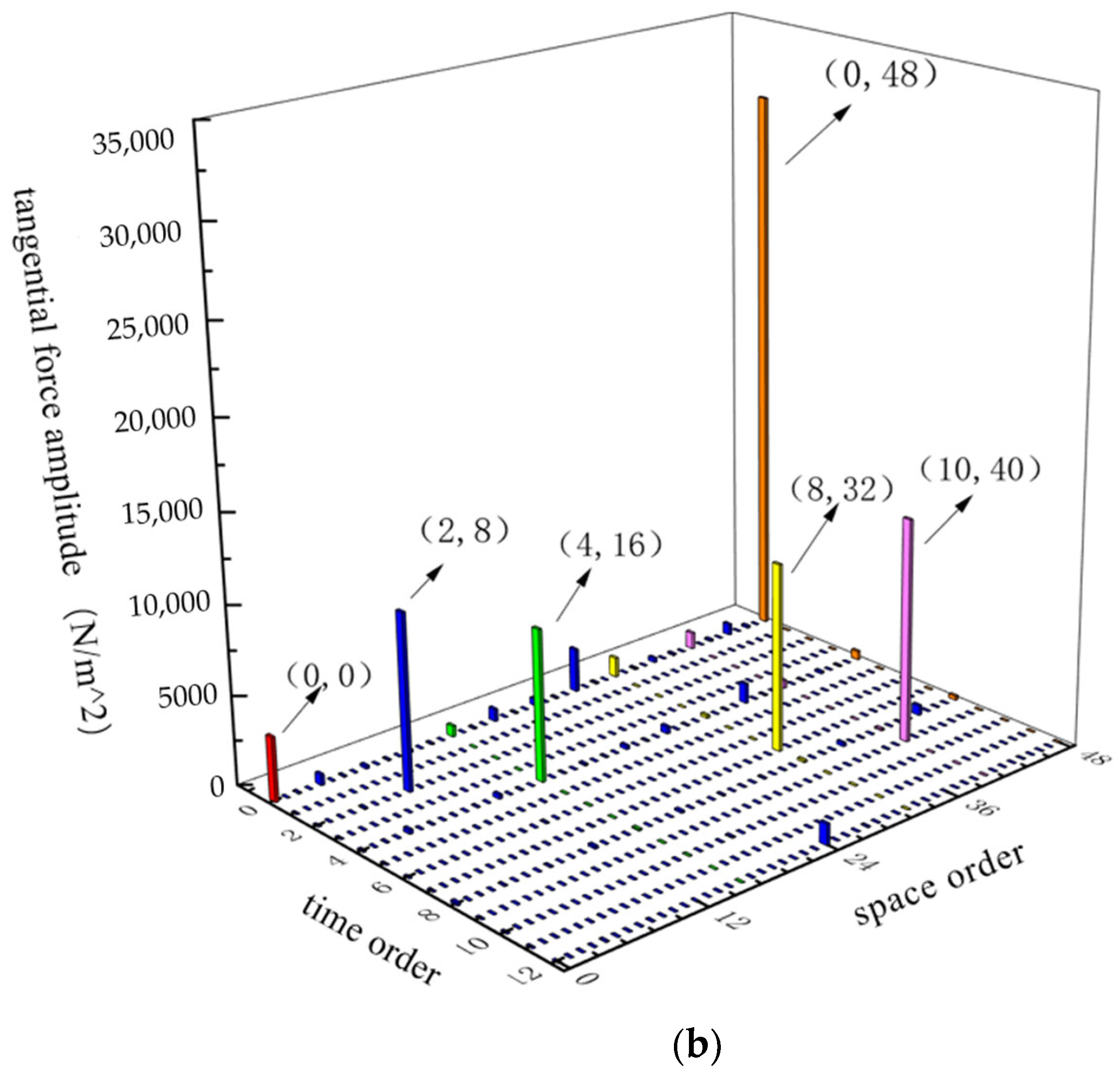
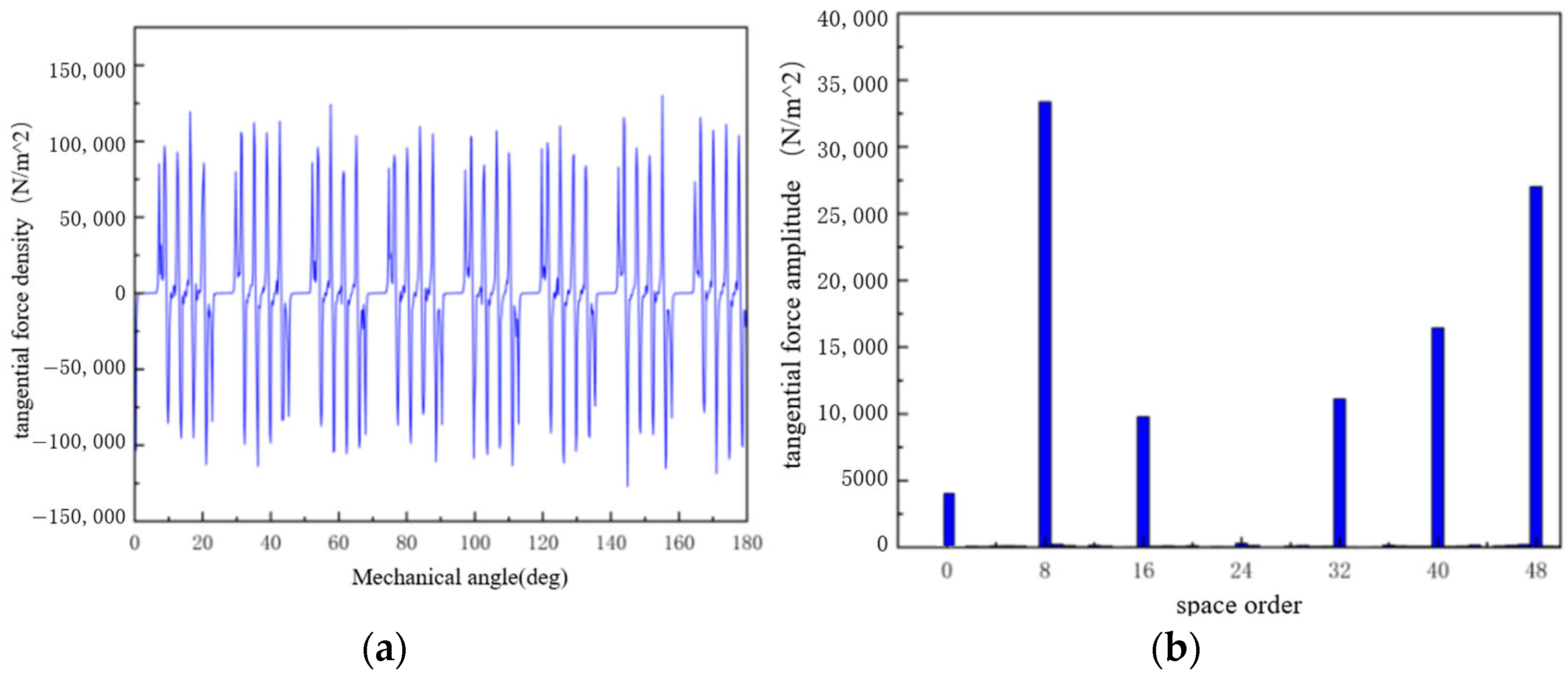
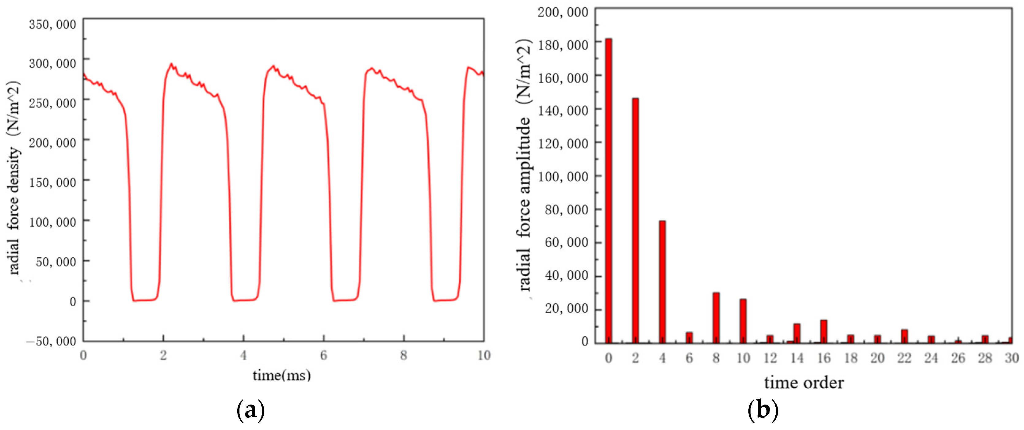
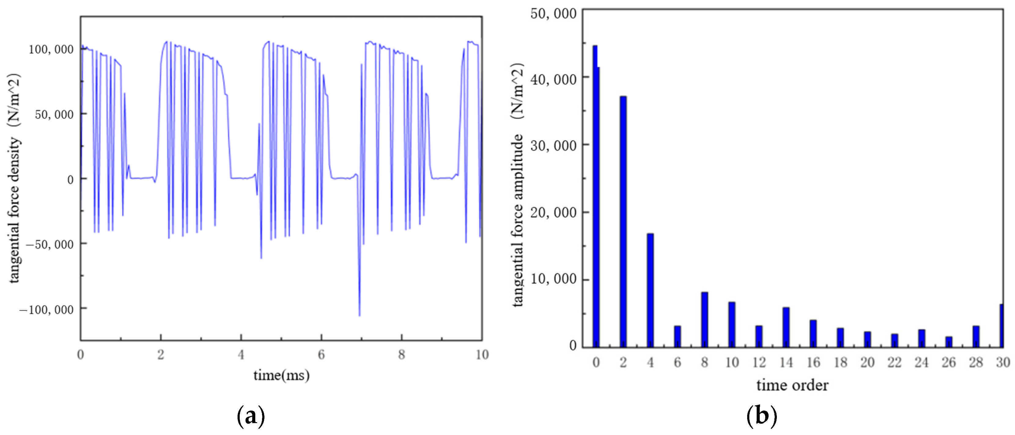
Under load operation, current excitation is adopted with the amplitude of the three-phase sinusoidal excitation current set to 24 A. The spatial distributions of the on-load radial and tangential electromagnetic force densities are shown in Figure 12a and Figure 13a, respectively; the temporal distributions in Figure 14a and Figure 15a, respectively; the spatial FFT spectra in Figure 12b and Figure 13b, respectively; and the temporal FFT spectra in Figure 14b and Figure 15b, respectively.

It can be observed from Figure 12, Figure 13, Figure 14 and Figure 15 that under load operation, the armature reaction magnetic field superimposes on the permanent magnet magnetic field. The radial and tangential force waves involve interactions among permanent magnet harmonics, armature reaction harmonics, and slot permeance harmonics. Finite element results indicate that the harmonic composition under load conditions remains consistent with the theoretical family of orders under no-load conditions, although the amplitudes of certain components may change due to the alteration of air-gap flux density distribution by the current magnetic field. For the motor under study, the dominant force wave components remain associated with the low-order harmonic family determined by the pole–slot combination. Therefore, radial force waves remain the dominant excitation source of electromagnetic vibration under load conditions. Tangential force waves mainly contribute to the average torque and torque ripple. It can also be found that the amplitude of the zeroth-order tangential electromagnetic force under load is much larger than that under no-load conditions, because the zeroth-order tangential electromagnetic force produces cogging torque under no-load conditions, whereas it produces average torque under load conditions. The on-load output torque is shown in Figure 16; by comparing Figure 11 and Figure 16, it can be seen that the on-load output torque amplitude is much larger than that under no-load conditions. This distinction is of great importance: suppressing torque ripple does not necessarily suppress radial vibration unless the radial force wave amplitude and its coupling with the modes are simultaneously reduced.

Combining the above spatial–temporal characteristics, the spatial–temporal waveforms and two-dimensional FFT spectra of the radial and tangential electromagnetic force waves under load are plotted in Figure 17 and Figure 18, respectively.

It can be seen from the above figures that the electromagnetic force waves under load contain the same harmonic components as those under no-load. Neglecting the influence of high-order force waves, the radial electromagnetic force with $r=8$ and $f=2$ exhibits the largest amplitude under both no-load and load conditions; therefore, priority attention should be given to the radial electromagnetic force with low spatial order.

5. Stator Modal Analysis

5.1. Modal Characteristics of Free Stator-Core

A three-dimensional stator model is established and imported into the ANSYS Workbench modal analysis module. In addition to the structural parameters of the motor, the material properties also affect the natural frequencies. Therefore, material parameters such as the density, Poisson’s ratio, and Young’s modulus of the PMSM must be determined during the modal analysis. Considering that in actual manufacturing, the stator core is usually formed by stacking silicon steel sheets along the axial direction to reduce eddy current losses, the motor stator is not a materially continuous elastic body. If each individual silicon steel sheet were meshed, the computational load would be extremely large. Since the change in radial stiffness after lamination is relatively small and its influence on modal analysis can be neglected, the stator core can be equivalently modeled as a continuous elastic body [15] to simplify the model and reduce computation time in finite element analysis. Its laminated characteristics can be accounted for by assigning anisotropic material parameters available in ANSYS Workbench. The material parameters of the stator core used in the simulations of this section are listed in

Table 4. Material parameters of the stator core.

Component	Material	Density (kg/m3)	Poisson’s Ratio	Young’s Modulus (Pa)	Shear Modulus (Pa)
Stator core	Silicon steel sheet	7850	0.3	$E_X=E_Y=E_Z=2\times {10}^{11}$	$G_{XY}=G_{XZ}=G_{YZ}=7.69\times {10}^{10}$

.

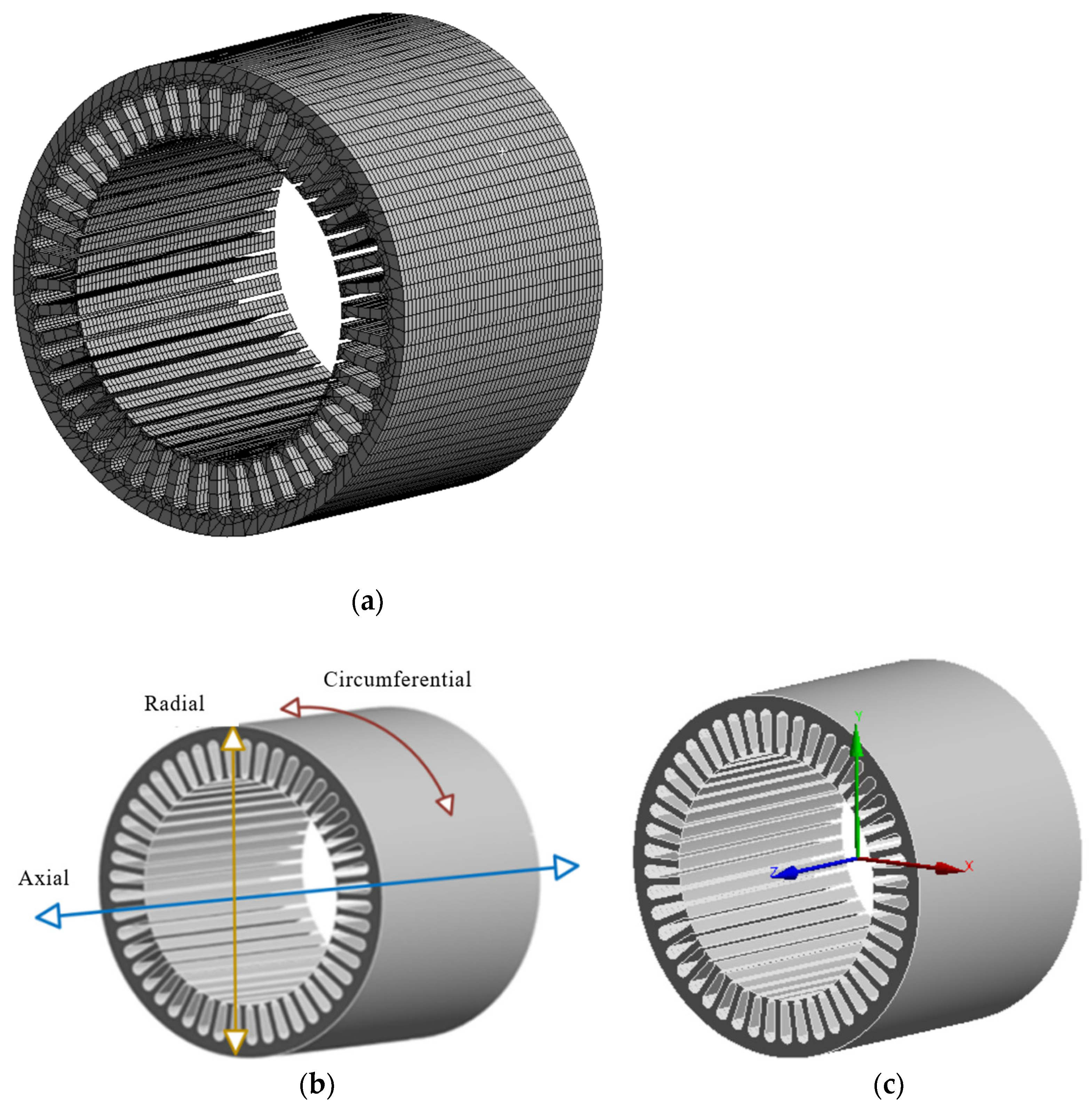
When conducting modal analysis, both computational accuracy and computational time must be comprehensively considered; therefore, an appropriate number of mesh elements must be selected. In this section, the stator core is meshed with a 5 mm element size, resulting in a total of 338,948 nodes and 65,484 elements, with an average element quality of 0.862, which satisfies the accuracy requirements for stator modal analysis. The meshing results are shown in Figure 19a. To investigate the modal shapes of the stator in greater depth, the concepts of circumferential, axial, and radial directions are distinguished here. As shown in Figure 19b, the circumferential direction refers to the peripheral direction along the outer surface of the stator cylindrical shell; together with the axial and radial directions, these constitute the three orthogonal directions of a cylindrical coordinate system. The axial direction is the direction of the stator rotation center axis, i.e., the direction passing through the center of the stator cylindrical end face and perpendicular to it. The radial direction is perpendicular to the axial direction and passes through the axis centerline, i.e., the diameter direction of the cylindrical end face.

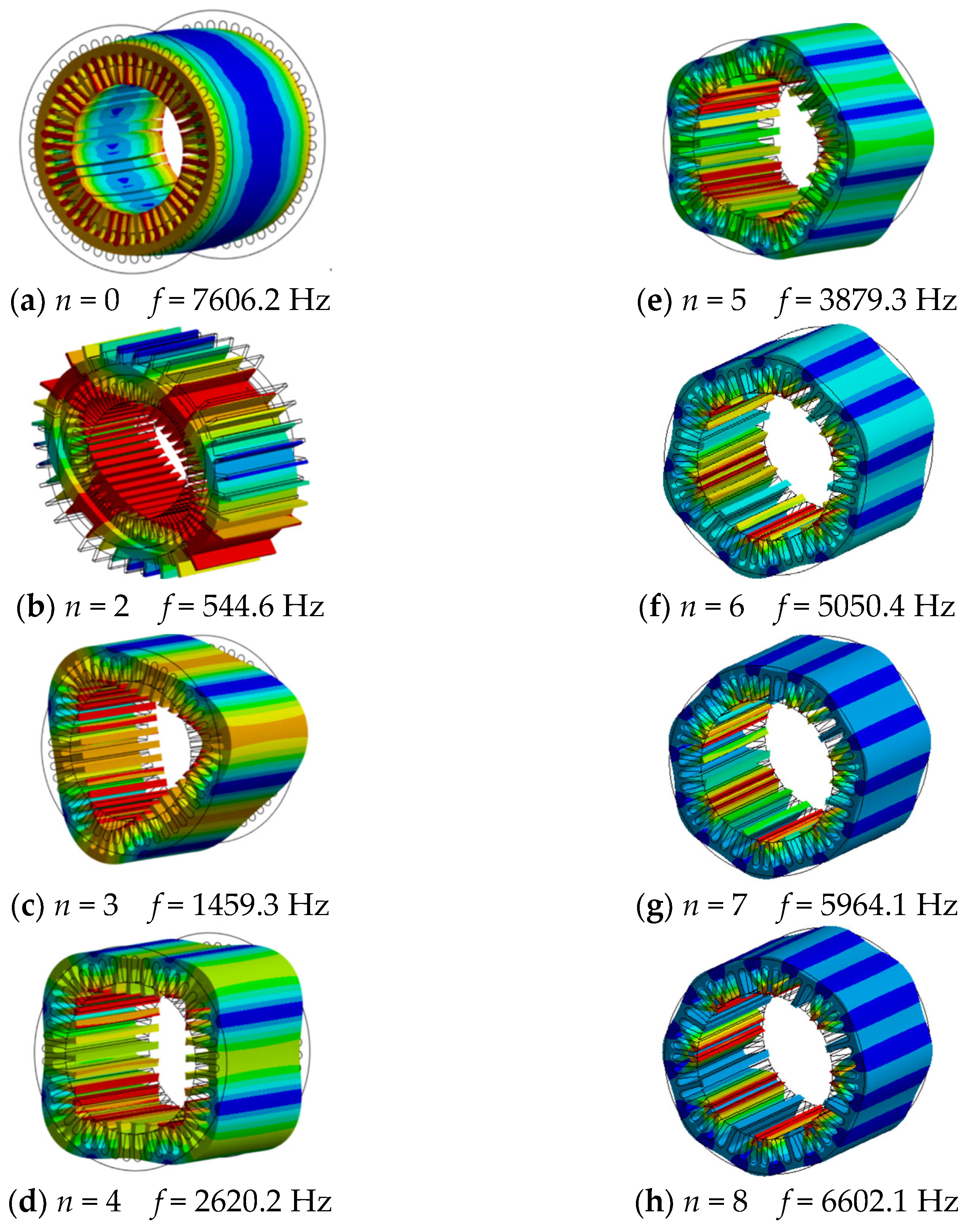
In the axial direction of the stator, the radial electromagnetic force wave is approximately uniformly distributed due to the symmetry of the air-gap magnetic field and does not excite significant axial modes. The natural frequencies of stator axial modes are usually far beyond the main frequency range of electromagnetic force waves and thus do not cause axial resonance. The lower-order radial force waves are most likely to have shapes similar to those of low-order circumferential modes of the stator; therefore, modal analysis focuses on circumferential deformation rather than axial deformation, meaning the axial order is 0. Since the minimum non-zero order of the radial electromagnetic force wave is 8, the modal analysis in this study mainly examines the mode shapes from order 0 to order 8, as shown in Figure 20. In the figure, colors closer to red represent greater displacement, while colors closer to blue represent smaller displacement.

The modal shapes shown in Figure 20 exhibit distinct geometric characteristics: the second-order mode is elliptical, the third-order mode is triangular, and the fourth- to eighth-order modes are corresponding polygons. Except for the zeroth-order breathing mode, the natural frequencies increase with the circumferential mode order. The frequency spacing between adjacent modes also increases with the order, indicating that low-order modes possess higher modal density and greater broadband resonance risk. Therefore, resonance avoidance requires examination of two aspects: first, frequency avoidance, meaning the excitation frequency should not approach the natural frequency; and second, mode shape avoidance, meaning the spatial distribution of electromagnetic force waves should not match the structural mode shapes. If a certain force component is strongly coupled with a low-damping structural mode, vibration may be induced even with a low amplitude; conversely, if the spatial coupling is weak, a component with a higher amplitude may not necessarily cause significant effects.

5.2. Modal Characteristics of Stator Assembly

To further investigate the influence of the motor housing on the stator modes, the housing is added to the stator in the Workbench modal analysis module to form the stator assembly. The contact relationship between the stator core and the housing is set to bonded, because in actual assembly the stator and housing are interference-fitted and no relative displacement occurs between them. The material parameters of the stator assembly are listed in

Table 5. Material parameters of the stator assembly.

Component	Material	Density (kg/m3)	Poisson’s Ratio	Young’s Modulus (Pa)	Shear Modulus (Pa)
Stator core	Silicon steel sheet	7850	0.3	$E_X=E_Y=E_Z=2\times {10}^{11}$	$G_{XY}=G_{XZ}=G_{YZ}=7.69\times {10}^{10}$
Housing	Aluminium alloy	2770	0.33	$E_X=E_Y=E_Z=7.1\times {10}^{10}$	$G_{XY}=G_{XZ}=G_{YZ}=2.69\times {10}^{10}$

.

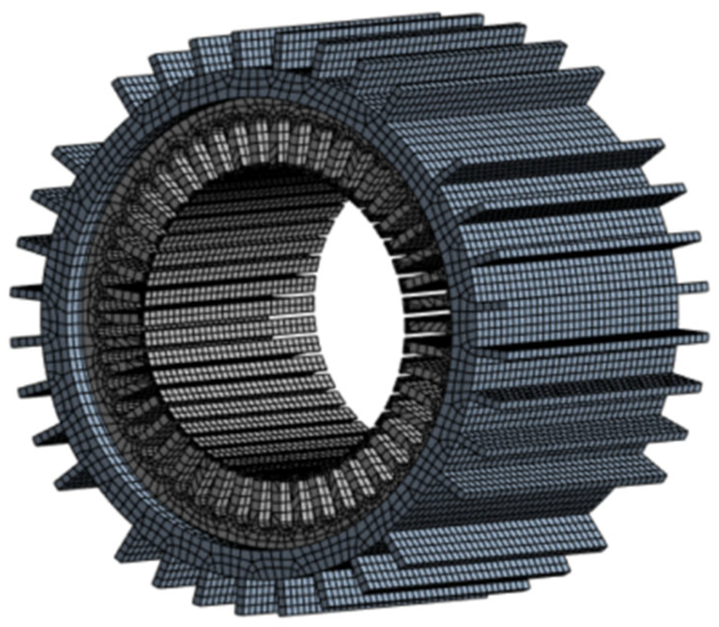
This subsection adopts the same meshing method as the previous subsection, with the stator assembly meshed using a 5 mm element size to ensure consistency in the computational results. The final mesh contains 315,639 nodes and 68,888 elements, with an average element quality of 0.847, which satisfies the accuracy requirements. The meshing results are shown in Figure 21.

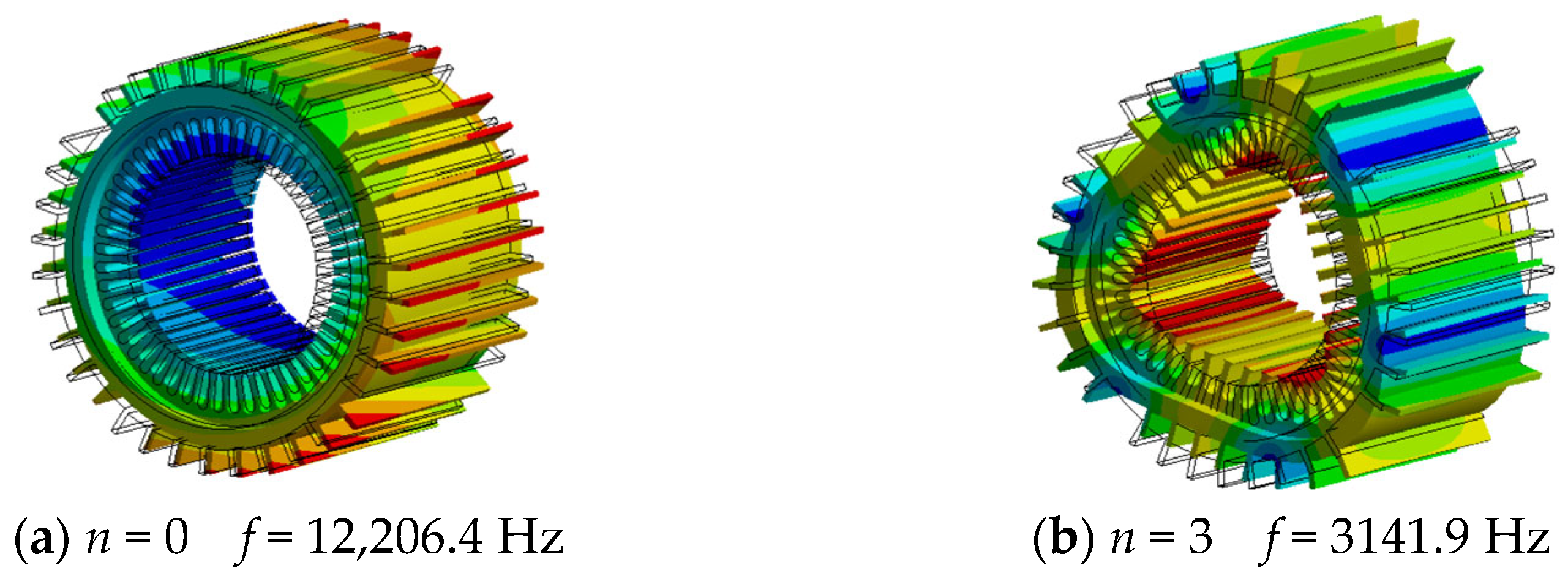
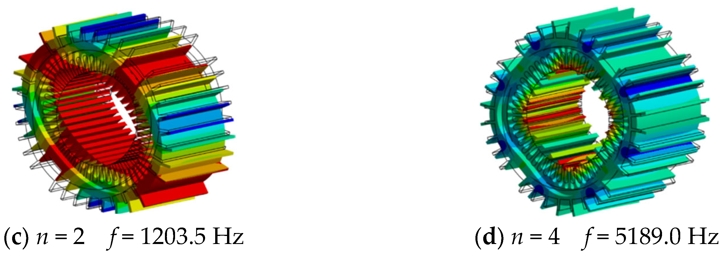
Modal analysis is performed on the stator assembly. Since its circumferential mode shapes are similar to those of the free stator core, only the first four orders are presented here, as shown in Figure 22. The zeroth- to eighth-order modal frequencies of the stator assembly compared with those of the free stator core are listed in

Table 6. Comparison of natural frequencies between the two models.

Axial Mode Order	Circumferential Mode Order	Stator Core	Stator Assembly	Absolute Difference	Relative Change
0	0	7606.2 Hz	12,206.4 Hz	4600.2 Hz	60.48%
	2	544.6 Hz	1203.5 Hz	658.9 Hz	120.98%
	3	1459.3 Hz	3141.9 Hz	1682.6 Hz	117.72%
	4	2620.2 Hz	5189.0 Hz	2568.8 Hz	98.03%
	5	3879.3 Hz	6735.2 Hz	2855.9 Hz	73.62%
	6	5050.4 Hz	8757.4 Hz	3707.0 Hz	73.40%
	7	5964.1 Hz	9864.0 Hz	3899.9 Hz	65.39%
	8	6602.1 Hz	10,488.1 Hz	3886.0 Hz	58.86%

. In the figure, colors closer to red represent greater displacement, while colors closer to blue represent smaller displacement.

It can be seen from the above table that the presence of the housing enhances the structural stiffness of the motor, raising the circumferential modal natural frequencies of the stator core. Applying constraints to the stator also enhances the stator stiffness to a certain extent. Moreover, the influence of the housing on the stiffness of the stator core is far greater than its influence on mass, thereby increasing the natural frequencies and making resonance less likely to occur. At the same time, it can be found that the housing has a greater effect on the low-order natural frequencies of the motor, while its influence on the high-order modal frequencies is relatively small.

6. Electromagnetic Vibration Simulation Analysis and Experimental Validation

6.1. No-Load Electromagnetic Vibration Simulation

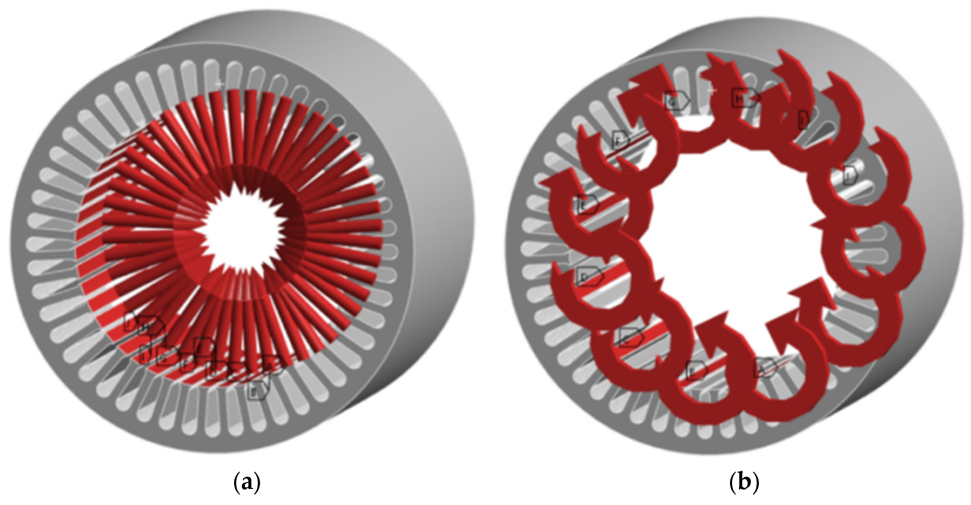
To calculate the vibration characteristics of the motor under electromagnetic forces, transient dynamic analysis is performed on the motor. To facilitate rapid analysis and computation, the free stator from the previous section is adopted as the simulation object in this section. First, the three-dimensional structural field model of the motor free stator is imported into the ANSYS harmonic response module; subsequently, the no-load electromagnetic force data obtained from Maxwell are coupled into the harmonic response module. After processing, the electromagnetic force waves are imported as loads in the harmonic response analysis module. Figure 23 illustrates the manner in which electromagnetic forces and electromagnetic torque are applied to the stator tooth surfaces.

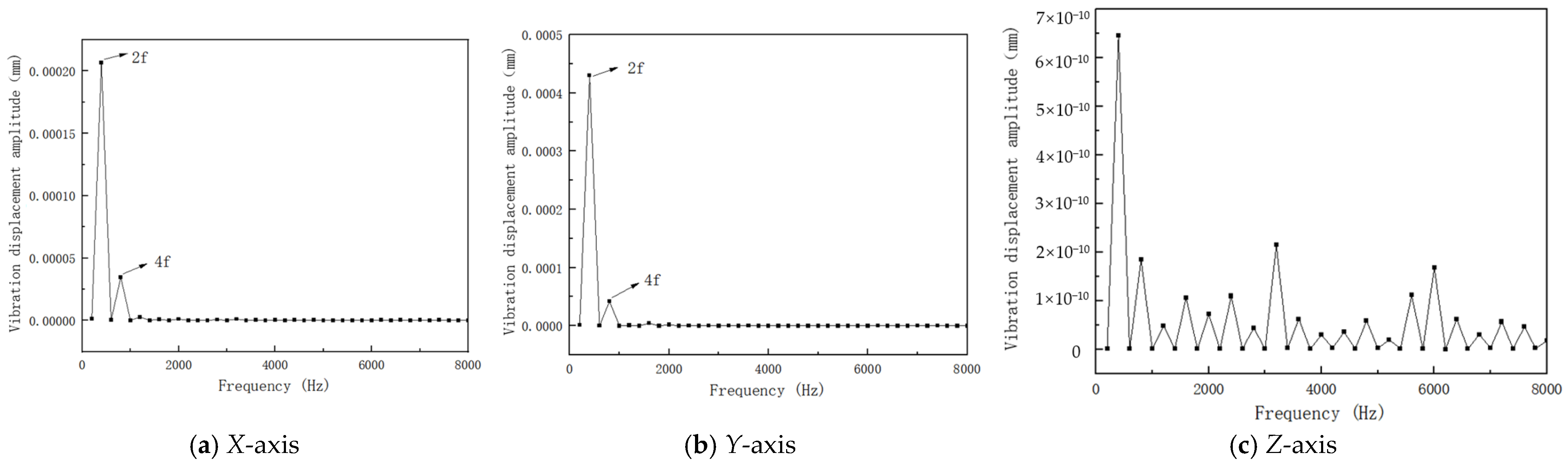
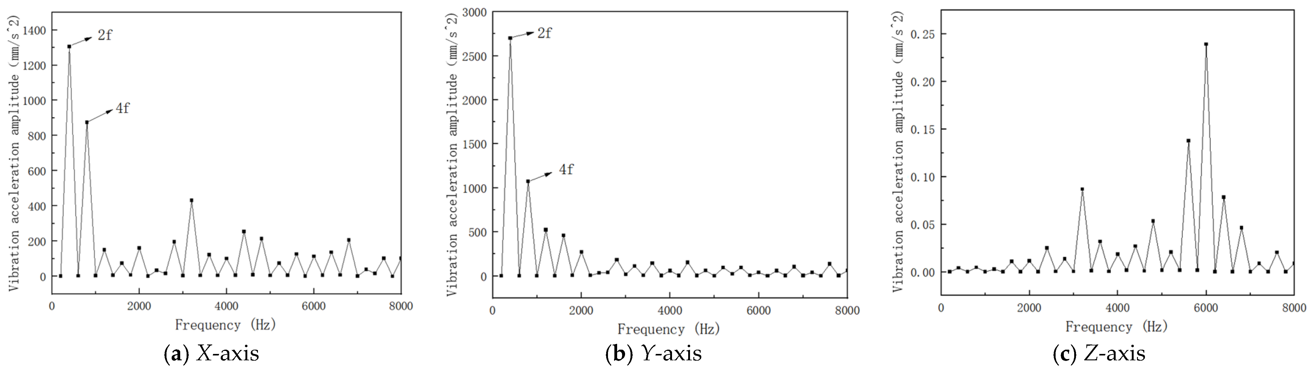
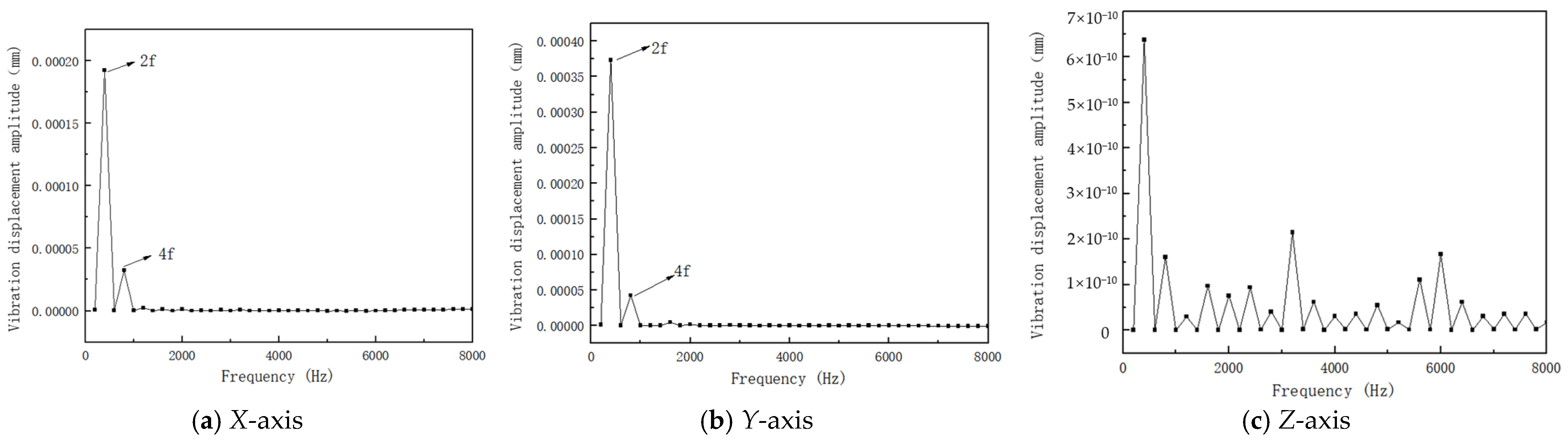
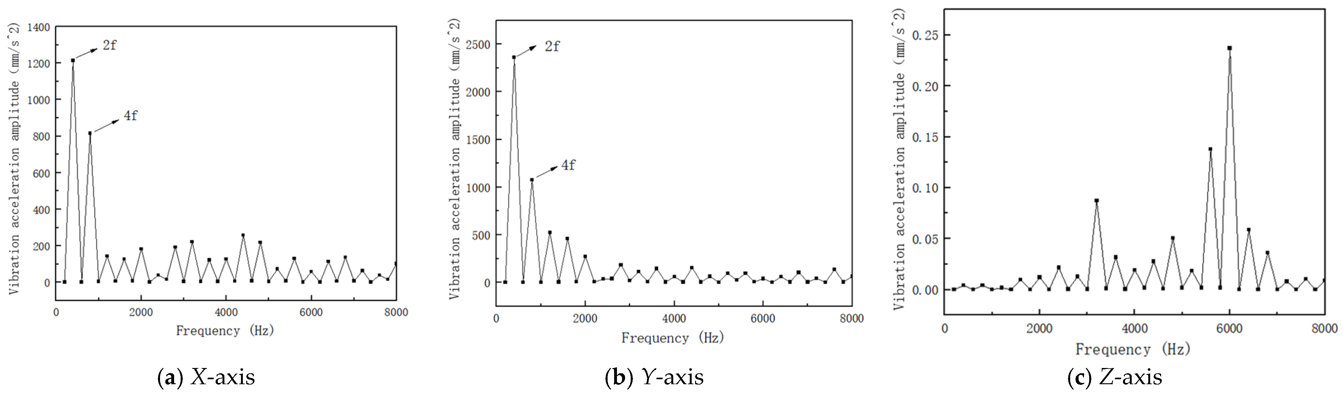
The modal superposition method is employed to simulate and analyze the motor vibration at the rated speed of 3000 rpm. It can be obtained from $f={\displaystyle \frac{np}{60}}$ that the fundamental frequency of the 48-slot 8-pole permanent magnet synchronous motor is 200 Hz. To ensure the accuracy of frequency-domain analysis, including the zeroth- to eighth-order modal frequencies, the solver is configured with a frequency range from 0 to 8000 Hz and a step interval of 200 Hz, i.e., one fundamental frequency. A point on the back of the motor stator core is selected as the vibration reference, and the amplitude-frequency characteristics of vibration displacement along the X, Y, and Z directions are shown in Figure 24; the amplitude-frequency characteristics of vibration acceleration are shown in Figure 25.

It can be observed from Figure 24 and Figure 25 that the vibration displacement and vibration acceleration amplitudes in the x and y directions are much larger than those in the z direction. Since the x and y directions are radial and the z direction is axial, the simulation results validate the conclusion that motor electromagnetic vibration is primarily radial vibration caused by radial electromagnetic force waves. The vibration acceleration reaches extrema at even harmonics, because the temporal orders of radial electromagnetic forces are all even, and their frequencies correspond to even multiples of the current fundamental frequency f. Therefore, vibration occurs in the motor at even multiples of the current fundamental frequency. Moreover, the vibration accelerations in the X and Y directions are relatively large at 2f and 4f, which corresponds to the FFT results of radial electromagnetic force waves obtained in Section 3, where the amplitudes of the 8th-order electromagnetic force at 2f and the 16th-order electromagnetic force at 4f are large. That is, these two vibrations are mainly caused by the radial electromagnetic forces (8, 2f) and (16, 4f).

6.2. Loaded Electromagnetic Vibration Simulation

The load electromagnetic force data obtained from Maxwell are coupled into the harmonic response module, with all other settings remaining consistent with the no-load electromagnetic vibration simulation in the previous subsection.

It can be observed from Figure 24, Figure 25, Figure 26 and Figure 27 that, regardless of whether the motor operates under no-load or load conditions, the vibration components with large amplitudes appear at even harmonic frequencies. Under load conditions, the armature reaction only increases the amplitude of motor vibration, making the motor vibration more severe, but does not change the vibration frequencies. Moreover, the vibration peaks under both no-load and load conditions occur at 400 Hz and 800 Hz, i.e., the second and fourth harmonic frequencies, among which the second harmonic is the most severe, corresponding to the frequency of the eighth-order radial electromagnetic force, indicating that the eighth-order electromagnetic force makes the dominant contribution to motor vibration. The 4th harmonic is the next largest, corresponding to the 16th-order electromagnetic force.

6.3. Experimental Testing

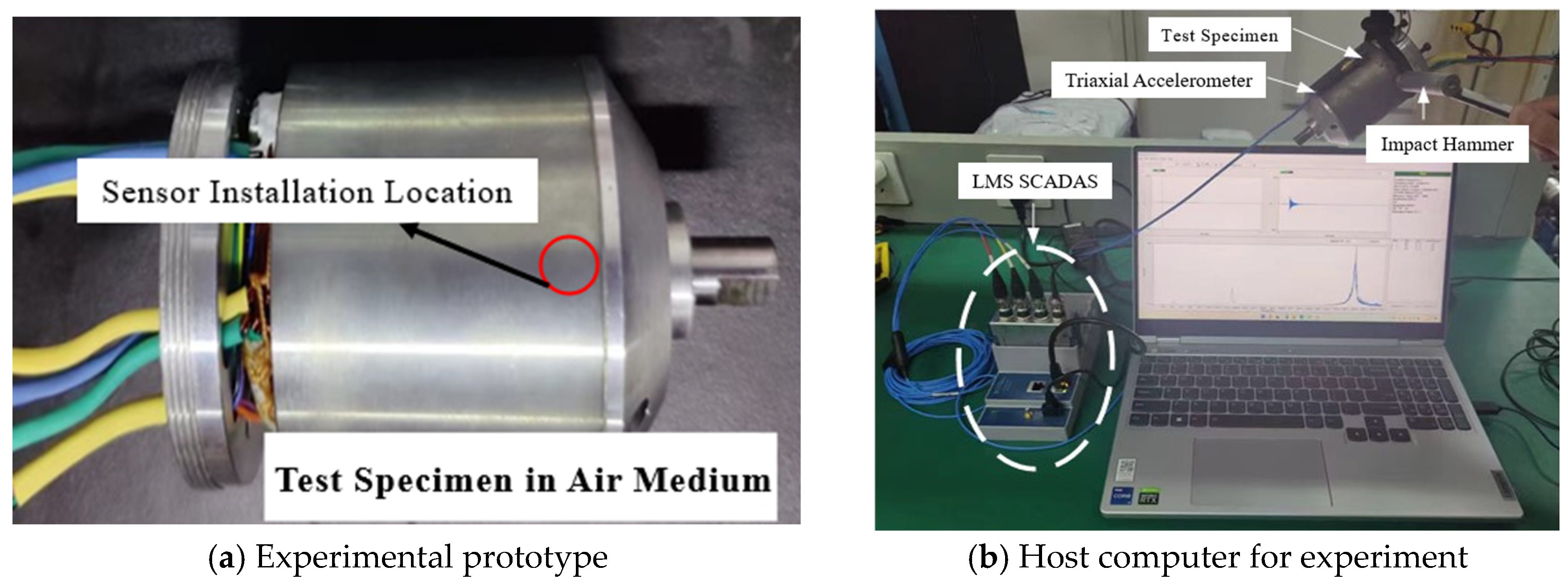
To verify the correctness of the simulation results and the applicability of the theoretical analysis conclusions, electromagnetic vibration tests on the permanent magnet synchronous motor prototype were carried out in an anechoic chamber; the experimental platform is shown in Figure 28. A triaxial accelerometer (model B&K 4535-B (HBK, Nærum, Denmark)) with a sensitivity of 1.0 mV/ms² was mounted on the motor surface at the same location as the point selected in the simulation analysis of the previous section. The signals collected by the sensor were fed into an LMS SCADAS data acquisition system (Siemens AG, Munich, Germany) and subsequently uploaded to the Simcenter Testlab software for analysis. The discrete time-domain signals acquired by the accelerometer are not conducive to analysis and comparison; therefore, the LMS SCADAS performs Fourier decomposition on the time-domain signals collected by the accelerometer to convert them into continuous frequency-domain signals, which are then transmitted to the Simcenter Testlab software. The amplitude-frequency characteristics of the vibration acceleration can thus be obtained. Since the motor in the simulation was in an unconstrained free modal state—an ideal condition that cannot be realized in practice—the motor was suspended using soft rubber ropes with low stiffness to simulate free boundary conditions, and the modal parameters were measured using the impact hammer method.

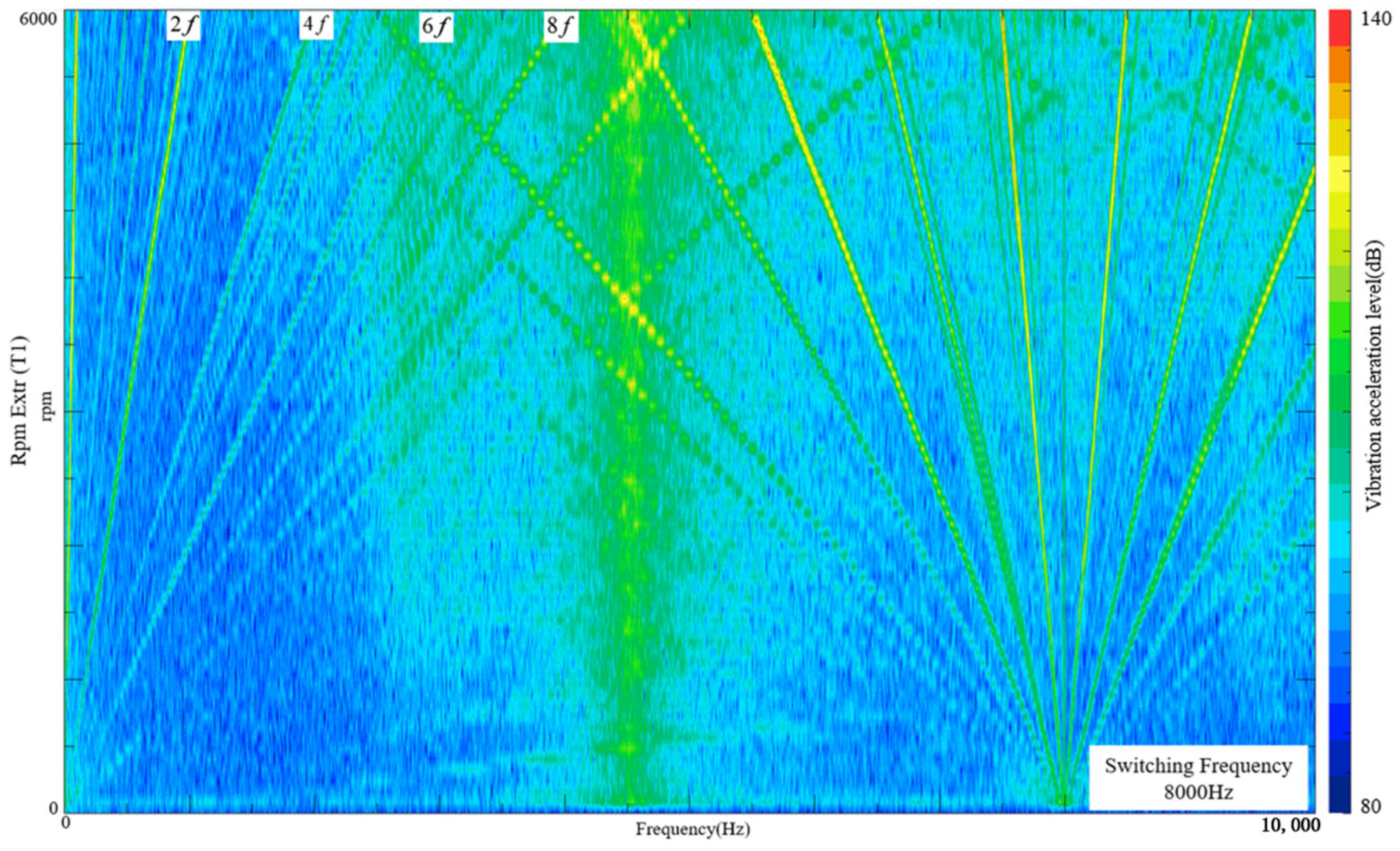
The experiments were conducted under the motor no-load condition, with the motor controller switching frequency set to 8 kHz. First, a multi-speed run-up vibration test from 0 to 6000 rpm was performed, with the acceleration ramp rate set to 150 rpm/s, a sampling frequency range of 0–10 kHz, and a step size of 5 Hz. During the motor run-up process, the vibration acceleration amplitude can vary by several orders of magnitude. A linear scale cannot simultaneously display weak and strong vibrations with clarity, whereas a logarithmic scale compresses this large dynamic range into a single plot. According to Equation (13), the root-mean-square (rms) value of vibration acceleration (in mm/s²) can be converted into the vibration acceleration level (in dB) [20]:

$$L_a=20\cdot {\log }_{10}\left({\displaystyle \frac{a_{\mathrm{rms}}}{a_0}}\right)$$

(14)

where $L_a$ denotes the vibration acceleration level; $a_{\mathrm{rms}}$ denotes the rms value of vibration acceleration, and $a_0={10}^{-6}{\mathrm{m}/\mathrm{s}}^2$ denotes the reference acceleration.

During the run-up process, the accelerometer measures the vibration acceleration at each rotational speed; the data acquisition system converts it into frequency-domain signals, and the Testlab software stacks the spectra according to rotational speed to obtain the multi-speed equivalent vibration acceleration level waterfall plot in the radial (Y-axis) direction, as shown in Figure 29. In Figure 29, the horizontal axis represents frequency, the left vertical axis represents rotational speed (unit: rpm), the right vertical axis represents the equivalent acceleration level (unit: dB), and the brighter the color, the stronger the vibration energy at that speed–frequency point.

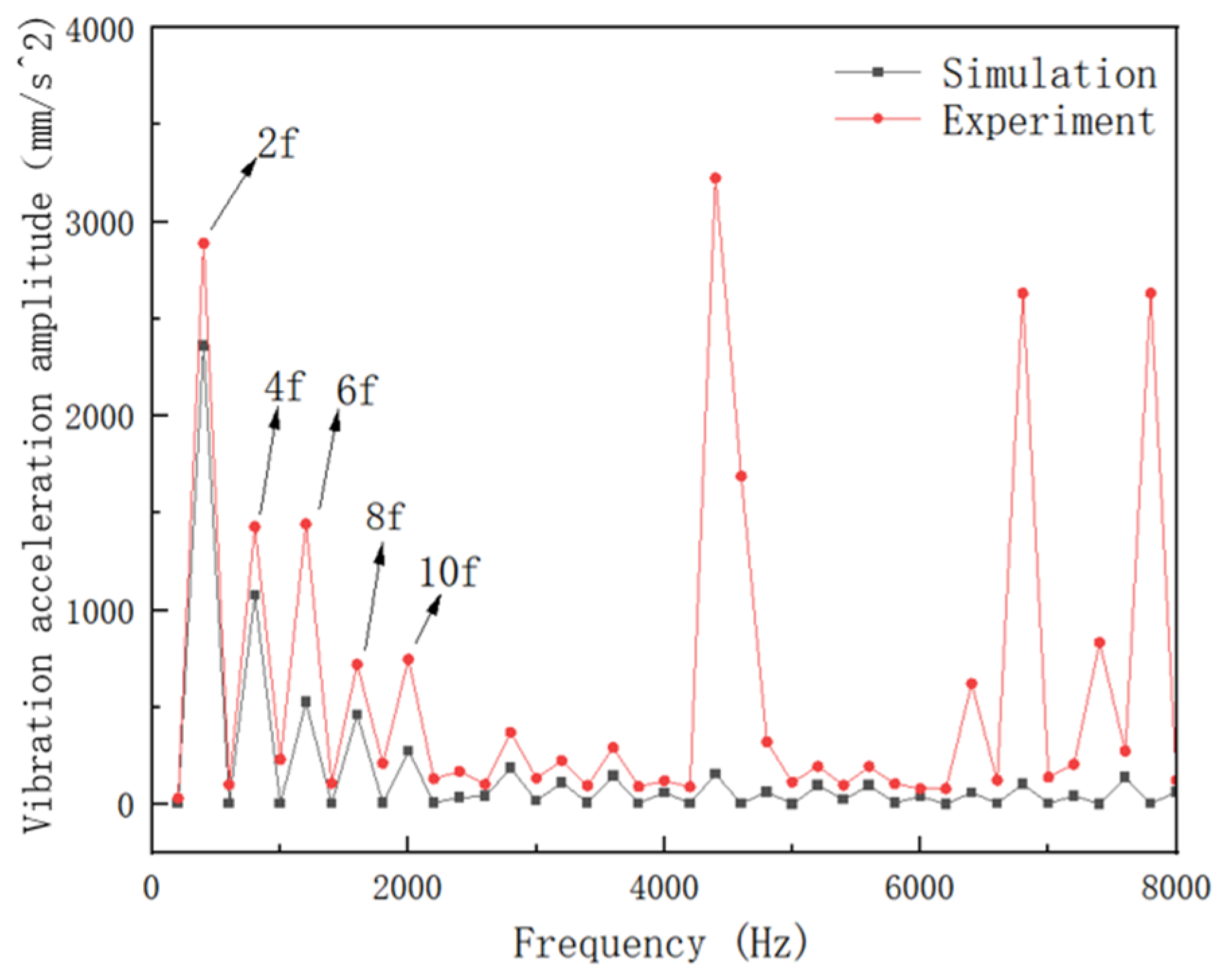
Subsequently, with the motor speed stabilized at 3000 rpm, the collected steady-state vibration signals were converted into vibration acceleration amplitudes and compared with the simulation results, as shown in Figure 30.

6.4. Experimental Results Analysis

It can be seen from Figure 29 that the bright bands distributed radially around 8000 Hz cause high-frequency vibration, which is related to the switching frequency. It can also be observed that vertical bright bands appear near 4500 Hz, indicating that this frequency band is close to the motor modal frequency and excites resonance. In the low-frequency region, the bright bands corresponding to large vibration still appear at even harmonics such as the second, fourth, sixth, and eighth multiples of the fundamental frequency; this trend is consistent with the conclusions obtained from the previous analysis. It is also noted that certain odd-harmonic bright bands exist; this is because during actual testing, the motor is affected by the modulation strategy, and sideband current harmonics excite sideband electromagnetic forces, thereby causing sideband vibration [21,22]. Since this paper only discusses electromagnetic vibration caused by radial electromagnetic force waves, vibration induced by the switching frequency and sideband current is not investigated in depth.

It can be observed from Figure 30 that both simulation and experiment show large vibration acceleration amplitudes at even harmonics; the simulation and measured results from the 2nd to the 10th harmonics are compared, as shown in

Table 7. Comparison of motor vibration acceleration between simulation results and experimental results.

Frequency (Hz)	Simulation Result (mm/s2)	Experimental Result (mm/s2)	Absolute Error (mm/s2)	Relative Error
400 (2f)	2359.6	2889.3785	529.7785	18%
800 (4f)	1075.4	1429.12	353.72	25%
1200 (6f)	24.1	943.204	919.104	97%
1600 (8f)	459.8	719.48	259.68	36%
2000 (10f)	273.1	746.28	473.18	63%

.

In Table 7, the absolute error is defined as the absolute value of the difference between the simulation result and the experimental result; the relative error is defined as the ratio of the absolute error to the experimental result. There is a certain discrepancy between the simulated and measured motor vibration acceleration results; in particular, a relatively large resonance occurs near 4500 Hz, which was not observed in the finite element simulation. This is because the measured motor vibration results are influenced not only by electromagnetic excitation forces but also by various factors such as mechanical structure, instrument installation, and fixation. Moreover, the simulation model in this paper inevitably simplifies damping, assembly interfaces, bearing constraints, housing details, and inverter control effects, and only considers the effect of radial electromagnetic forces while neglecting tangential electromagnetic forces and torque ripple. However, the main low-frequency vibration trends are basically consistent; it can be seen that the vibrations at the second and fourth harmonics are electromagnetic vibrations caused by radial electromagnetic force waves.

As mentioned previously, this paper only discusses electromagnetic vibration caused by radial electromagnetic force waves, and certain simplifications have been made to the model. This finite element model can be used for preliminary design evaluation of PMSMs and rapid prediction of electromagnetic vibration, providing researchers with a convenient research approach and methodology. Future research will focus on the aspects neglected in the previous work to improve model accuracy and more accurately reflect the vibration behavior of the motor, thereby providing guidance for the suppression and optimization of motor vibration.

7. Motor Vibration Mitigation and Optimization

The mechanical impedance theory provides a theoretical basis for the relationship between electromagnetic forces and mechanical vibration. The theoretical analysis of multi-degree-of-freedom forced vibration and the vibration equations for motor systems have been elaborated in Section 3. When the motor stator is regarded as a cylindrical shell, the vibration displacement caused by the r-th order radial electromagnetic force acting on it can be expressed as [23]

$$A_{\mathrm{m}}={\displaystyle \frac{F_k/M}{\sqrt{{\left({\omega }_i^2-{\omega }_k^2\right)}^2+4{\zeta }_i^2{\omega }_k^2{\omega }_i^2}}}$$

(15)

where $F_k$ denotes the k-th order radial electromagnetic force; $M$ is the equivalent mass of the stator core, windings, and housing; ${\omega }_i$ and ${\zeta }_i$ are the i-th order natural frequency and damping ratio, respectively; and ${\omega }_k$ is the frequency of the k-th order radial electromagnetic force. It can be seen from Equation (15) that the vibration displacement $A_{\mathrm{m}}$ of the motor is proportional to the amplitude of the radial electromagnetic force density causing the vibration. Moreover, according to reference [17], when considering only the circumferential modes of the stator core, the vibration displacement of the stator core is inversely proportional to the fourth power of the spatial order of the force wave, and the vibration is most severe when the frequency of the radial electromagnetic force wave approaches the natural frequency of the stator. Meanwhile, Equation (15) provides two approaches for vibration suppression: one starting from the electromagnetic force wave, and the other from the structural modal characteristics of the motor. To date, according to the specific implementation principles, vibration and noise reduction methods based on structural improvement can be roughly classified into three categories: modal planning, electromagnetic force amplitude optimization, and electromagnetic force effect optimization [21]. This section will investigate how to optimize the motor design and suppress electromagnetic vibration by analyzing the factors influencing modal frequencies and electromagnetic force amplitudes.

7.1. Analysis of the Influence of Different Structural Parameters on Stator Modes

Treating the stator as a thin cylindrical shell, its natural frequency can be calculated by the following equation [24]:

$$\left.\begin{array}{l}{f}_0={\displaystyle \frac{1}{\mathrm{\pi }{D}_c}}\sqrt{{\displaystyle \frac{E}{\rho \Delta }}}\\ \Delta =1+{\displaystyle \frac{m_t+m_w}{m_c}}\end{array}\right\}$$

(16)

where $f_0$ is the zeroth-order breathing mode frequency; $D_c$ is the diameter of the stator ring; $\rho$ is the material density of the stator ring; $E$ is the Young’s modulus of the stator material; $\Delta$ is the mass addition coefficient; $m_t$ is the mass of the stator yoke; $m_w$ is the mass of the windings; and $m_c$ is the mass of the stator teeth. When the modal order $n\ge 2$, the natural frequency expression for the single-ring model is

$$\left.\begin{array}{l}{f}_n=f_0{\displaystyle \frac{i\left(n^2-1\right)n}{\sqrt{n^2+1}}}{\displaystyle \frac{1}{\sqrt{1+\frac{i^2\left(n^2-1\right)\left[n^2\left(4+\frac{{\Delta }_n}{\Delta }\right)+3\right]}{n^2+1}}}}\\ i={\displaystyle \frac{h_c}{\sqrt{3}{D}_c}}\\ {\Delta }_n=1+{\displaystyle \frac{Z{\theta }_t}{\mathrm{\pi }{D}_{c}I}}\\ {\theta }_t=(\Delta -1)S_t{h}_t^3\left[{\displaystyle \frac{1}{3}}+{\displaystyle \frac{h_c}{2h_t}}+{\left({\displaystyle \frac{h_c}{2h_t}}\right)}^2\right]\\ I={\displaystyle \frac{L{h}_c^3}{12}}\end{array}\right\}$$

(17)

where $i$ is a proportional coefficient; ${\Delta }_n$ is the rotational mass increase coefficient; $h_c$ is the height of the stator core yoke; $h_t$ is the height of the stator core teeth; $S_t$ is the average cross-sectional area of the stator teeth; and $L$ is the length of the stator core. It can be seen from Equation (16) that the natural frequency of the stator is related to the stator axial length, stator yoke thickness, and stator mean radius. In this section, based on the stator cylindrical shell theory, simulations are conducted to analyze these three factors individually to investigate their influence on stator modes. The simulation comparisons adopt the single-variable method; the stator material parameters are the same as those in Table 4, and the influences of windings, housing, and end covers are not considered. All simulations presented in this section were conducted under no-load conditions.

7.1.1. Analysis of the Influence of Axial Length on Stator Modes

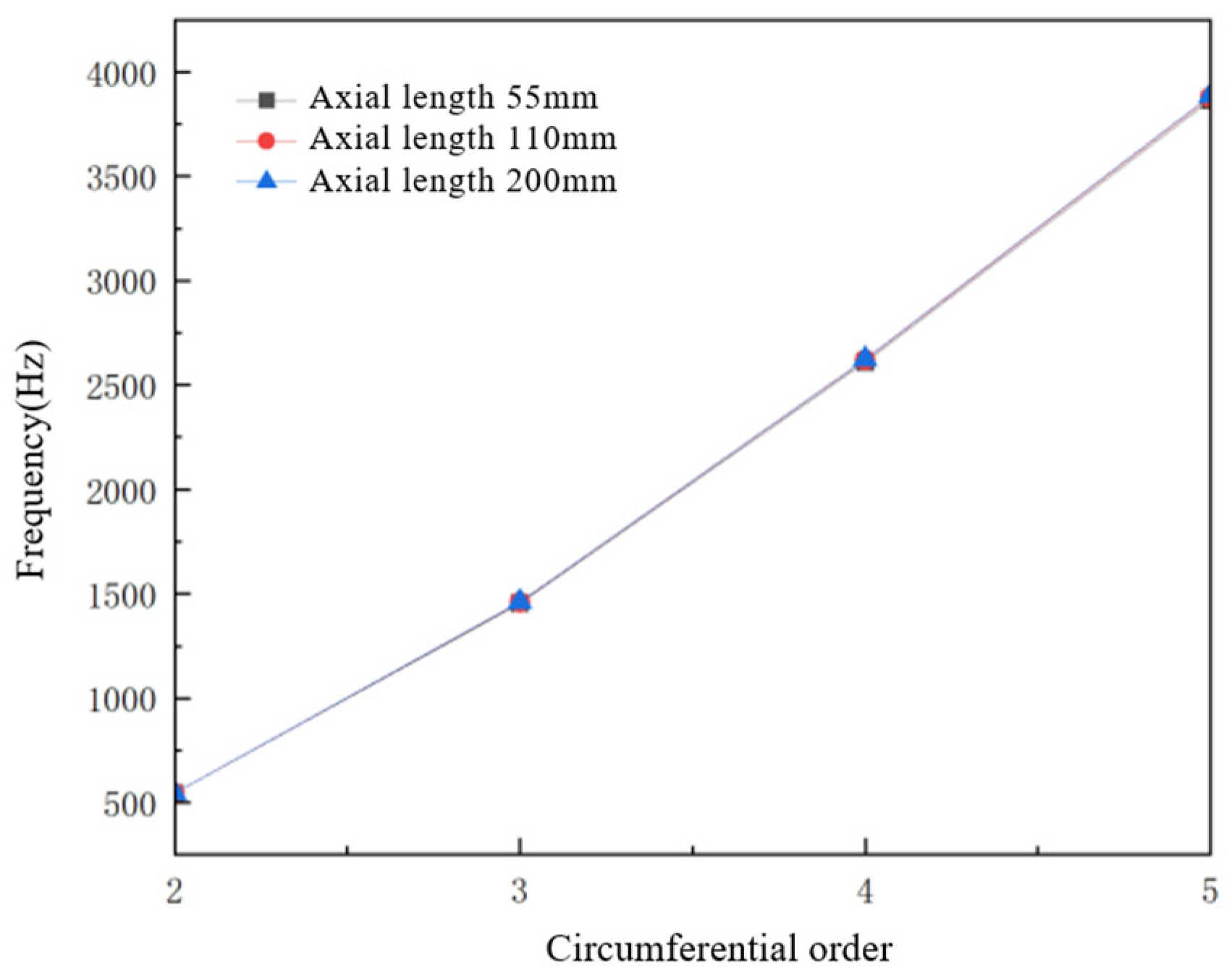
With the stator inner diameter fixed at 105 mm, outer diameter at 155 mm, and yoke thickness at 6.3 mm, only the stator axial length is varied. Axial lengths of 55 mm, 110 mm, and 200 mm are selected, and the natural frequencies of each mode are obtained through modal simulation. The comparison results are shown in

Table 8. Comparison of natural frequencies for different axial lengths.

Axial Length	n = 2	Relative Change Rate	n = 3	Relative Change Rate	n = 4	Relative Change Rate	n = 5	Relative Change Rate
55 mm	544.2 Hz	0	1452.7 Hz	0	2608.9 Hz	0	3863.5 Hz	0
110 mm	544.62 Hz	0.11%	1459.3 Hz	0.45%	2620.2 Hz	0.43%	3879.3 Hz	0.41%
200 mm	545.42 Hz	0.22%	1461.3 Hz	0.59%	2623.7 Hz	0.57%	3885.8 Hz	0.58%

and Figure 31.

It can be seen from Table 8 and Figure 31 that changing the stator axial length does not produce significant changes in the stator natural frequencies; that is, variations in stator axial length do not alter the natural frequencies of the stator circumferential modes.

7.1.2. Analysis of the Influence of Yoke Thickness on Stator Modes

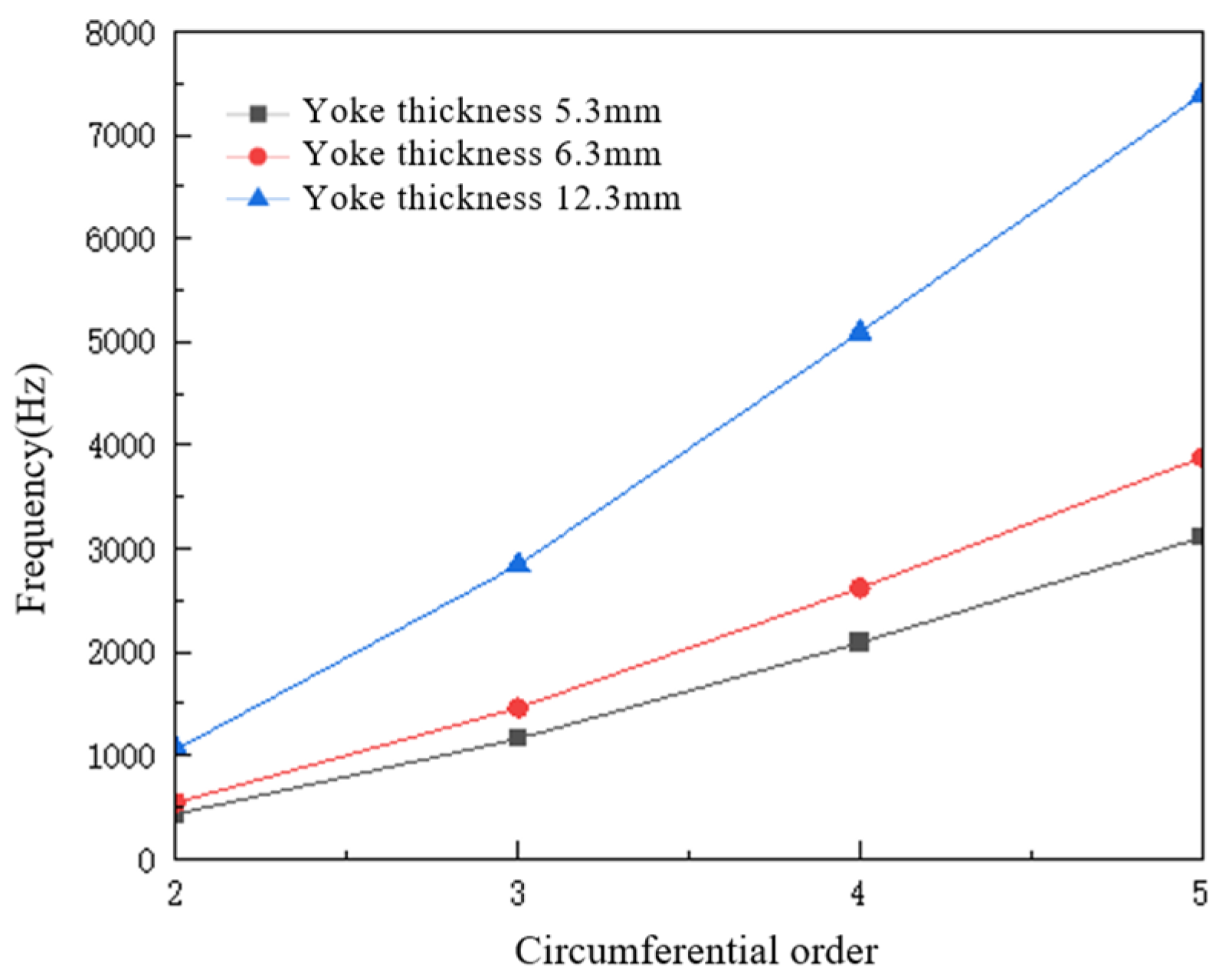
With the stator inner diameter fixed at 105 mm, outer diameter at 155 mm, and axial length at 110 mm, only the stator yoke thickness is varied. Yoke thicknesses of 5.3 mm, 6.3 mm, and 12.3 mm are selected, and the natural frequencies of each mode are obtained through modal simulation. The comparison results are shown in

Table 9. Natural frequencies for different yoke thicknesses.

Yoke Thickness	n = 2	n = 3	n = 4	n = 5
5.3 mm	434.77 Hz	1162.4 Hz	2088.5 Hz	3108.8 Hz
6.3 mm	544.62 Hz	1459.3 Hz	2620.2 Hz	3879.3 Hz
12.3 mm	1056.4 Hz	2841.5 Hz	5088.4 Hz	7386.1 Hz

and Figure 32.

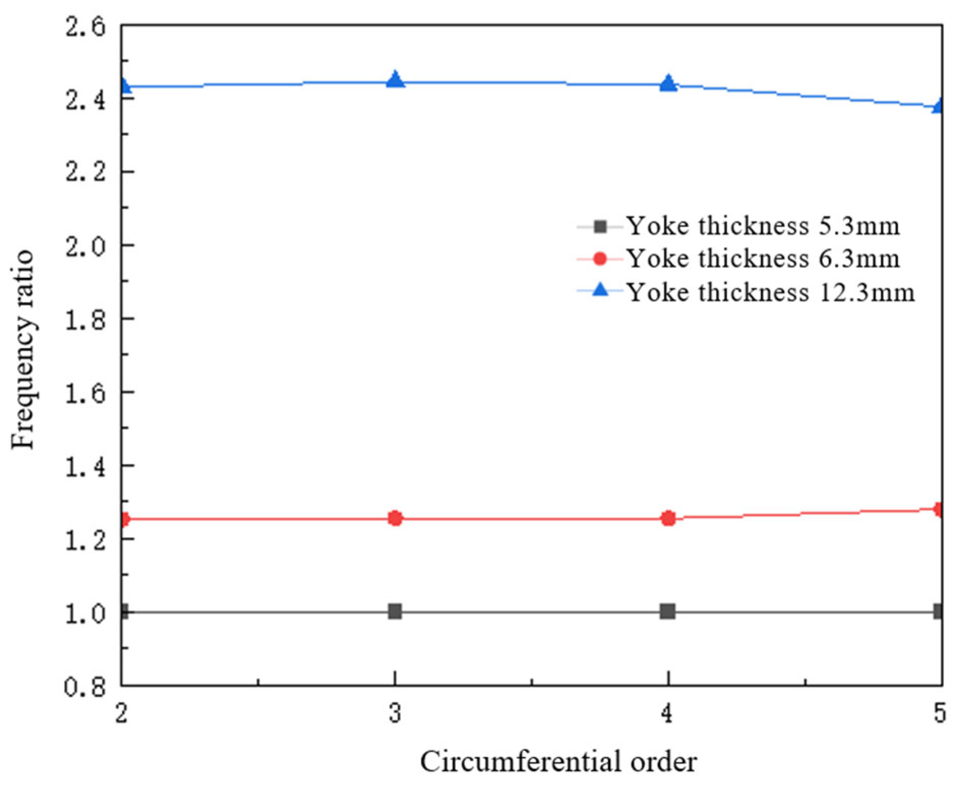
It can be seen from

Table 10. Natural frequency ratios for different yoke thicknesses.

Yoke Thickness	n = 2	n = 3	n = 4	n = 5	d1/d2
5.3 mm	434.77 Hz	1162.4 Hz	2088.5 Hz	3108.8 Hz	1
6.3 mm	1.253	1.255	1.255	1.248	1.189
12.3 mm	2.430	2.445	2.436	2.376	2.321

and Figure 33 that the frequency ratio for different yoke thicknesses is approximately equal to the ratio of their yoke thicknesses, that is

$${\displaystyle \frac{f_{r1}}{f_{r2}}}\approx {\displaystyle \frac{d_1}{d_2}}$$

(18)

where $f_{r1}$ and $f_{r2}$ are the r-th order natural frequencies, and $d_1$ and $d_2$ are different yoke thicknesses. This relationship exhibits deviation at higher-order modes.

7.1.3. Analysis of the Influence of Stator Diameter on Stator Modes

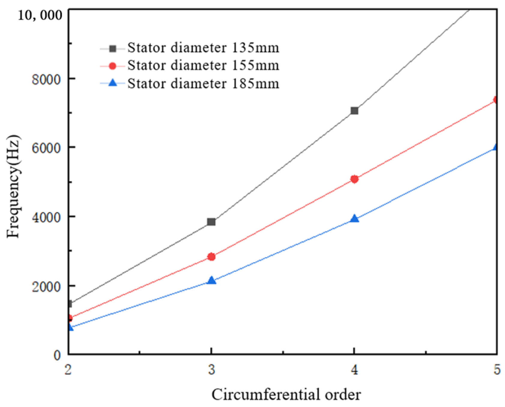
With the stator axial length fixed at 110 mm and the yoke thickness at 12.3 mm, only the stator diameter is varied. Stator diameters of 135 mm, 155 mm, and 185 mm are selected, with the inner diameter, slot opening width, slot depth, and other corresponding parts scaled proportionally. The natural frequencies of each mode are obtained through modal simulation, and the comparison results are shown in

Table 11. Comparison of natural frequencies for different stator diameters.

Stator Diameter	n = 2	n = 3	n = 4	n = 5
135 mm	1	1	1	1
155 mm	1056.4 Hz	2841.5 Hz	5088.4 Hz	7386.1 Hz
185 mm	783.28 Hz	2134.6 Hz	3920.3 Hz	6016.8 Hz

and Figure 34.

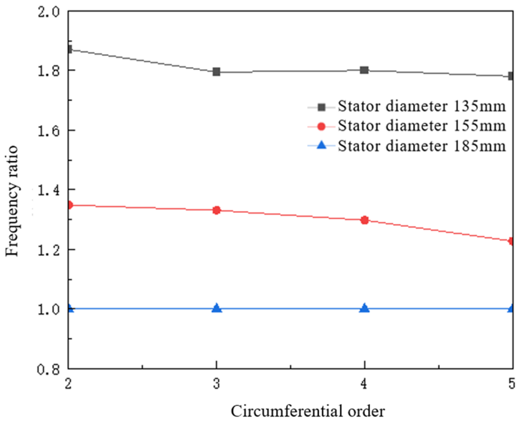
It can be seen from Table 11 and Figure 34 that as the stator diameter decreases, the circumferential modal natural frequencies of the stator increase accordingly. This is because a smaller stator diameter leads to increased curvature of the stator shell and enhanced in-plane stiffness. To further identify the quantitative relationship, the modal frequencies of each order under the three diameters are divided by the corresponding modal frequencies at a diameter of 185 mm to obtain the frequency ratios for different diameters, as shown in

Table 12. Natural frequency ratios for different diameters.

Stator Diameter	n = 2	n = 3	n = 4	n = 5	D22/D12
135 mm	1.870	1.794	1.800	1.780	1.877
155 mm	1.349	1.331	1.298	1.227	1.425
185 mm	1	1	1	1	1

and Figure 35.

It can be seen from Table 12 and Figure 35 that the frequency ratio for different stator outer diameters is approximately inversely proportional to the square of the outer diameter, that is

$${\displaystyle \frac{f_{r1}}{f_{r2}}}\approx {\displaystyle \frac{D_2^2}{D_1^2}}$$

(19)

where $f_{r1}$ and $f_{r2}$ are the r-th order natural frequencies, and $D_1$ and $D_2$ are different stator outer diameters. This relationship exhibits deviation at higher-order modes.

The above results have direct design implications. Increasing the yoke thickness can shift key modal frequencies away from electromagnetic excitation frequencies, but simultaneously increases mass and material costs. Reducing the stator diameter can increase natural frequencies, but may conflict with electromagnetic torque and cooling requirements. The axial length has very little effect on circumferential modal frequencies in this model and therefore should not be regarded as a primary parameter for avoiding circumferential electromagnetic resonance. Although varying the yoke thickness and stator diameter can optimize motor modal frequencies, from an economic cost perspective, the priority of changing these two parameters in actual production is not high, and the influence of other factors should be considered first.

7.2. Analysis of the Influence of Air-Gap Width on Electromagnetic Vibration

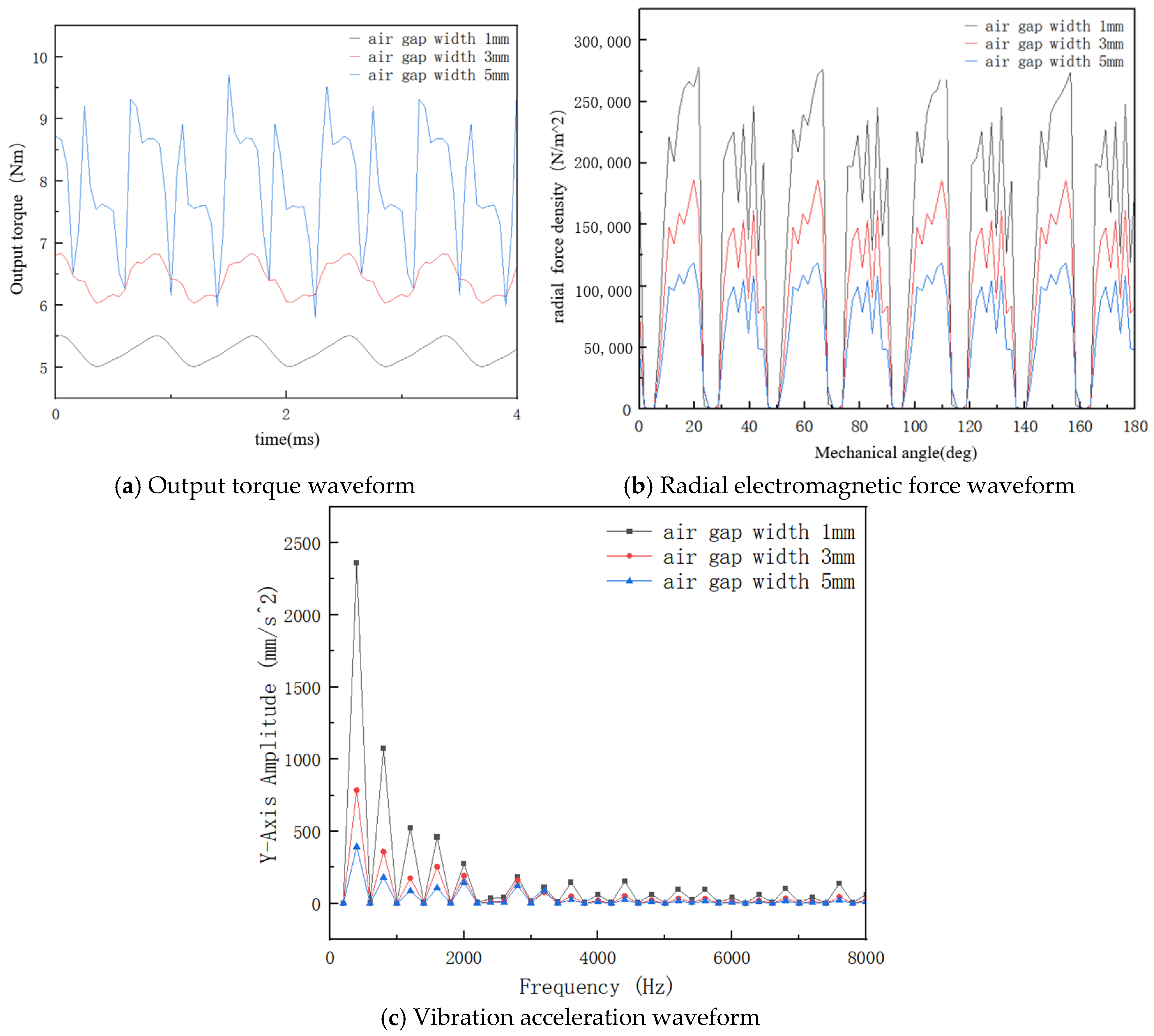
The air gap serves as the main magnetic field path, and its characteristics directly determine the electromagnetic performance, electromagnetic vibration, and efficiency of the motor. In this section, with the slot opening width fixed at 1.75 mm, the pole arc coefficient at 0.7, and all other parameters kept identical, air-gap widths of 1 mm, 3 mm, and 5 mm are selected to investigate the influence of air-gap width on motor torque, radial electromagnetic force waves, and electromagnetic vibration. The effects of varying the air-gap width on motor output torque, radial electromagnetic force amplitude, and radial vibration acceleration are shown in Figure 36a, b, and c, respectively.

It can be seen from Figure 36 that as the air-gap width increases, the motor torque, radial electromagnetic force density amplitude, and vibration acceleration all decrease accordingly. This is because the permeability of air is much lower than that of the permanent magnet; increasing the air-gap width enlarges the magnetic reluctance, thereby reducing the air-gap flux density, which in turn causes the radial electromagnetic force density and output torque to decrease. Meanwhile, an increase in air-gap width leads to a higher order of air-gap permeance harmonics, resulting in electromagnetic force waves with higher frequencies. Higher-order force waves are less likely to excite structural resonance in the motor, further reducing the vibration acceleration. Therefore, varying the air-gap width is a key means in motor design to balance electromagnetic performance and electromagnetic vibration: when a larger output torque is desired, the air-gap width can be appropriately reduced, but care must be taken to avoid rotor-to-stator rubbing caused by an excessively small air gap; when it is desired to reduce torque ripple, decrease the amplitude of electromagnetic force waves, and mitigate electromagnetic vibration, the air-gap width can be appropriately increased, but an excessively large width will cause a sharp drop in torque and degrade motor performance. Consequently, the adjustment of air-gap width requires comprehensive consideration of various factors to obtain optimal motor performance.

8. Conclusions

This paper takes an 8-pole 48-slot permanent magnet synchronous motor for unmanned underwater vehicles (UUVs) as the research object. Starting from the practical need for vibration and noise reduction, the electromagnetic vibration characteristics of the PMSM are systematically investigated, the causes of electromagnetic vibration are analyzed, and design schemes for motor vibration reduction and optimization are proposed. The main conclusions are as follows:

• First, derivation based on the Maxwell stress tensor method indicates that radial electromagnetic force waves are the primary source of stator electromagnetic vibration. For the studied 8-pole 48-slot motor, the minimum non-zero spatial force wave order is 8, and all other non-zero spatial orders are integer multiples thereof. The results obtained through finite element simulation and FFT analysis are consistent with the theoretical analysis.
• Second, a finite element simulation model of the permanent magnet synchronous motor was constructed. Simulation analyses of the air-gap magnetic field and electromagnetic force waves under both no-load and on-load conditions were carried out, verifying the feasibility of the analytical model and obtaining accurate spatial–temporal characteristics of the electromagnetic force waves, thereby providing reliable input for electromagnetic vibration calculation. Tangential force waves and radial force waves originate from the interaction of the same magnetic field and contain corresponding harmonic components; however, their primary mechanical effect is torque ripple rather than stator radial vibration, whereas the radial electromagnetic vibration of the motor is caused by radial electromagnetic force waves. Therefore, radial and tangential forces should be distinguished when evaluating vibration and torque ripple.
• Third, theoretical analysis and finite element simulation of the motor modal shapes were conducted, and the modal frequencies of each order for the free stator and the stator assembly were obtained. Different low-order circumferential stator modes have mode shapes similar to those of low-order radial force waves and are therefore more easily excited. Electromagnetic resonance avoidance should simultaneously consider both frequency matching and spatial mode shape matching.
• Fourth, electromagnetic vibration multi-physics coupling analysis and experimental verification were completed. Using finite element software Ansys 2023 R1, a multi-physics coupling simulation model integrating electromagnetics, magnetic forces, and structural vibration was constructed, and the vibration characteristics of the motor under no-load and on-load conditions were analyzed, leading to the conclusion that electromagnetic force waves are the main source of motor electromagnetic vibration. To verify the correctness of the theoretical analysis and finite element simulation model, motor vibration characteristic tests were carried out, and the experimental results were compared with the simulation results. Although a certain discrepancy exists between the simulated and measured vibration acceleration results, the main low-frequency vibration trends are basically consistent. Specifically, the vibrations at the second and fourth harmonic frequencies are electromagnetic vibrations induced by radial electromagnetic force waves, with relative errors between the measured and simulated values of 18% and 25%, respectively. The finite element model developed in this paper can be used for preliminary design evaluation of PMSMs and rapid prediction of electromagnetic vibration, providing researchers with a convenient research approach and methodology.
• Finally, starting from the stator vibration formula, the factors affecting electromagnetic vibration were discussed. By varying stator structural parameters to analyze their influence on stator modes, and by varying the air-gap width to analyze its influence on radial electromagnetic forces, the effects on electromagnetic vibration were further investigated, providing ideas and directions for optimizing motor design and suppressing electromagnetic vibration.

The analysis and suppression of motor vibration have always been a problem involving enormous workload and complexity. The simulations and experiments presented in this paper still have many aspects worthy of improvement, such as the influence of switching frequency on vibration, the influence of sideband harmonics on vibration, and the influence of low-frequency resonance. The authors will continue to conduct in-depth research on these issues in future work. In addition, changing the motor pole–slot combination to weaken cogging harmonics is also a research direction worth exploring.

References

1. Zhang, B.; Du, B.; Zhao, T.; Xiao, Y.; Cui, S. Overview of Research Status and Development of Ship Electric Propulsion Motors. Proc. CSEE 2022, 42, 7608–7623. (In Chinese) [Google Scholar]
2. Cui, G.; Xiong, B.; Huang, K.; Li, Z.; Ruan, L. Spatial Distribution Characteristics and Influencing Factors of Demagnetization of Permanent Magnet Motor for Electric Vehicle. Trans. China Electrotech. Soc. 2023, 38, 5959–5974. (In Chinese) [Google Scholar]
3. Zhang, Q.; Jia, Z.; Cheng, S.; Wang, D. Analysis and Calculation of Radial Electromagnetic Force of Circular Winding Brushless DC Motor. IEEE Trans. Ind. Electron. 2020, 67, 4338–4349. [Google Scholar] [CrossRef] [Scilit]
4. Dong, J.; Yin, H.; Li, G.; Wang, X.; Luo, M. The Multiphysics Analysis and Suppression Method for the Electromagnetic Noise of Permanent-Magnet Motors Used in Electric Vehicle. World Electr. Veh. J. 2025, 16, 136. [Google Scholar] [CrossRef] [Scilit]
5. Tang, R. Modern Permanent Magnet Motors—Theory and Design; China Machine Press: Beijing, China, 1997; pp. 1–3. (In Chinese) [Google Scholar]
6. Li, X.; Cheng, S.; Ren, Q.; Lü, Y.; Hu, L.; Xiao, F. Vibration Suppression Method for Slot-Frequency Breathing Mode of Large Permanent Magnet Synchronous Motors. Proc. CSEE 2026, 1–10. (In Chinese) [Google Scholar] [CrossRef]
7. Yang, H. Electromagnetic Vibration Analysis of Permanent Magnet Synchronous Motor. Ph.D. Thesis, Zhejiang University, Hangzhou, China, 2011; pp. 1–4. (In Chinese) [Google Scholar]
8. Lan, H. Research on Electromagnetic Force Waves and Electromagnetic Vibration of Permanent Magnet Synchronous Motor. Ph.D. Thesis, Harbin Institute of Technology, Harbin, China, 2019. (In Chinese) [Google Scholar]
9. Li, X.; Liu, C.; Mei, B.; Wei, S.; Xia, N. Analysis of Vibration and Noise Sources of IPMSM for Electric Vehicles in Wide Speed Range. Proc. CSEE 2018, 38, 5219–5227. (In Chinese) [Google Scholar] [CrossRef]
10. Fang, H.; Li, D.; Qu, R.; Yan, P. Modulation Effect of Slotted Structure on Vibration Response in Electrical Machines. IEEE Trans. Ind. Electron. 2019, 66, 2998–3007. [Google Scholar] [CrossRef] [Scilit]
11. Soresini, F.; Barri, D.; Ballo, F.; Manzoni, S.; Gobbi, M.; Mastinu, G. Noise, Vibration, and Harshness Countermeasures of Permanent Magnet Synchronous Motor with Viscoelastic Layer Material. SAE Int. J. Veh. Dyn. Stab. NVH 2025, 9, 537–554. [Google Scholar] [CrossRef] [Scilit]
12. Yin, H.; Hua, W.; Wu, Z.; Zhang, H. Fourier-Based Vibration Model of Electrical Machines Considering Nonideal Orthogonality between Electromagnetic Forces and Structural Modes. IEEE Trans. Ind. Electron. 2024, 71, 4485–4494. [Google Scholar] [CrossRef] [Scilit]
13. Chen, S.; Ding, S.; Shen, S.; Dai, Y.; Yang, Z. Electromagnetic Vibration Analysis and Suppression of Surface-Mounted Permanent Magnet Synchronous Motor for Ships. Trans. China Electrotech. Soc. 2023, 38, 1275–1286. (In Chinese) [Google Scholar] [CrossRef]
14. Xia, J.; Kang, L.; Zhan, Y.; Sun, Y.; Guo, M. Pole-Slot Radial Force Wave Compensation Model and Parameter Identification of Surface-Mounted Three-Phase Permanent Magnet Synchronous Motor. Trans. China Electrotech. Soc. 2021, 36, 1596–1606. (In Chinese) [Google Scholar] [CrossRef]
15. Xin, W. Research on Electromagnetic Performance and Vibration Noise Characteristics of Permanent Magnet Synchronous Motor for Electric Vehicles. Master’s Thesis, Harbin University of Science and Technology, Harbin, China, 2023. (In Chinese) [Google Scholar]
16. Liu, C.; Bai, H.; Zhuo, S.; Zhang, X.; Ma, R.; Gao, F. Real-Time Simulation of Power Electronic Systems Based on Predictive Behavior. IEEE Trans. Ind. Electron. 2019, 67, 8044–8053. [Google Scholar] [CrossRef] [Scilit]
17. Tsivitse, P.J.; Weishsmann, P.R. Polyphase Induction Motor Noise. IEEE Trans. Ind. Gen. Appl. 1971, 7, 339–358. [Google Scholar] [CrossRef] [Scilit]
18. Zou, J.; Lan, H.; Xu, Y.; Zhao, B. Analysis of Global and Local Force Harmonics and Their Effects on Vibration in Permanent Magnet Synchronous Machines. IEEE Trans. Energy Convers. 2017, 32, 1523–1532. [Google Scholar] [CrossRef] [Scilit]
19. Mao, Y.; Zuo, S.; Wu, X.; Duan, X. High Frequency Vibration Characteristics of Electric Wheel System under In-Wheel Motor Torque Ripple. J. Sound Vib. 2017, 400, 442–456. [Google Scholar] [CrossRef] [Scilit]
20. Zhang, Q.; Li, W.; Wang, C. The Fast Prediction of Sound Radiation from Typical Submarine Cabin Based on Acoustic Transfer Vector. In Proceedings of the 2016 IEEE/OES China Ocean Acoustics (COA), Harbin, China, 9–11 January 2016. [Google Scholar] [CrossRef] [Scilit]
21. Song, C.; Wu, Z.; Li, M.; Deng, W. Overview of Electromagnetic Vibration and Noise Research of Permanent Magnet Synchronous Motors. Trans. China Electrotech. Soc. 2026, 41, 1887–1906. (In Chinese) [Google Scholar]
22. Lin, F.; Zuo, S.; Deng, W.; Wu, S. Noise Prediction and Sound Quality Analysis of Variable-Speed Permanent Magnet Synchronous Motor. IEEE Trans. Energy Convers. 2017, 32, 698–706. [Google Scholar] [CrossRef] [Scilit]
23. Gieras, J.F.; Wang, C.; Lai, J.C. Noise of Polyphase Electric Motors; CRC Press: Boca Raton, FL, USA, 2018. [Google Scholar]
24. Wang, H. Research on Electromagnetic Noise and Vibration Characteristics of Interior Permanent Magnet Synchronous Motor for Electric Vehicles. Ph.D. Thesis, Zhejiang University, Hangzhou, China, 2021. (In Chinese) [Google Scholar]
Figure 1. Circumferential mode shapes of the equivalent single-ring stator model.
Applsci 16 08467 g001
Figure 3. Two-dimensional finite element model and boundary conditions of the 8-pole 48-slot PMSM and mesh division of the PMSM model.
Applsci 16 08467 g003
Figure 4. Contour plot of motor magnetic field distribution under no-load condition: magnetic flux density and magnetic vector potential. (a) PMSM flux density. (b) Magnetic vector potential and flux lines.
Applsci 16 08467 g004
Figure 5. No-load radial electromagnetic force density spatial distribution and FFT waveform. (a) No-load radial electromagnetic force density spatial distribution. (b) No-load radial electromagnetic force density spatial FFT waveform.
Applsci 16 08467 g005
Figure 6. No-load tangential electromagnetic force density spatial distribution and FFT waveform. (a) No-load tangential electromagnetic force density spatial distribution. (b) No-load tangential electromagnetic force density spatial FFT waveform.
Applsci 16 08467 g006
Figure 7. No-load radial electromagnetic force density temporal distribution and FFT waveform. (a) No-load radial electromagnetic force density temporal distribution. (b) No-load radial electromagnetic force density temporal FFT waveform.
Applsci 16 08467 g007
Figure 8. No-load tangential electromagnetic force density temporal distribution and FFT waveform. (a) No-load tangential electromagnetic force density temporal distribution. (b) No-load tangential electromagnetic force density temporal FFT waveform.
Applsci 16 08467 g008
Figure 9. Spatial–temporal waveforms of no-load radial and tangential electromagnetic force densities. (a) No-load radial electromagnetic force density. (b) No-load tangential electromagnetic force density.
Applsci 16 08467 g009aApplsci 16 08467 g009b
Figure 10. Two-dimensional FFT spectra of no-load radial and tangential electromagnetic forces. (a) Radial two-dimensional FFT. (b) Tangential two-dimensional FFT.
Applsci 16 08467 g010
Figure 11. No-load output torque.
Applsci 16 08467 g011
Figure 12. Load radial electromagnetic force density spatial distribution and FFT waveform. (a) Load radial electromagnetic force density spatial distribution. (b) Load radial electromagnetic force density spatial FFT waveform.
Applsci 16 08467 g012
Figure 13. Load tangential electromagnetic force density spatial distribution and FFT waveform. (a) Load tangential electromagnetic force density spatial distribution. (b) Load tangential electromagnetic force density spatial FFT waveform.
Applsci 16 08467 g013
Figure 14. Load radial electromagnetic force density temporal distribution and FFT waveform. (a) Load radial electromagnetic force density temporal distribution. (b) Load radial electromagnetic force density temporal FFT waveform.
Applsci 16 08467 g014
Figure 15. Load tangential electromagnetic force density temporal distribution and FFT waveform. (a) Load tangential electromagnetic force density temporal distribution. (b) Load tangential electromagnetic force density temporal FFT waveform.
Applsci 16 08467 g015
Figure 16. Load output torque.
Applsci 16 08467 g016
Figure 17. Spatial–temporal waveforms of load radial and tangential electromagnetic force densities. (a) Load radial electromagnetic force density. (b) Load tangential electromagnetic force density.
Applsci 16 08467 g017aApplsci 16 08467 g017b
Figure 18. Two-dimensional FFT spectra of load radial and tangential electromagnetic forces. (a) Radial two-dimensional FFT. (b) Tangential two-dimensional FFT.
Applsci 16 08467 g018aApplsci 16 08467 g018b
Figure 19. Schematic diagram of 3D stator model. (a) Schematic Diagram of Stator Core Mesh Discretization. (b) Schematic of Stator Circumferential, Axial and Radial Directions. (c) Cartesian Coordinate System.
Applsci 16 08467 g019
Figure 20. Mode shape diagram of free–free supported stator core.
Applsci 16 08467 g020
Figure 21. Mesh division of the stator assembly.
Applsci 16 08467 g021
Figure 22. Mode shapes of the stator assembly.
Applsci 16 08467 g022aApplsci 16 08467 g022b
Figure 23. Loading methods of electromagnetic force and electromagnetic torque. (a) Electromagnetic force loading method. (b) Electromagnetic torque loading method.
Applsci 16 08467 g023
Figure 24. Amplitude-frequency characteristics of no-load vibration displacement along X, Y, and Z axes.
Applsci 16 08467 g024
Figure 25. Amplitude-frequency characteristics of no-load vibration acceleration along X, Y, and Z axes.
Applsci 16 08467 g025
Figure 26. Amplitude-frequency characteristics of loaded vibration displacement along X, Y, and Z axes.
Applsci 16 08467 g026
Figure 27. Amplitude-frequency characteristics of loaded vibration acceleration along X, Y, and Z axes.
Applsci 16 08467 g027
Figure 28. On-site photographs of vibration experiment.
Applsci 16 08467 g028
Figure 29. Waterfall plot of equivalent vibration acceleration level under run-up condition.
Applsci 16 08467 g029
Figure 30. Comparison of Y-axis vibration acceleration between simulation and experiment.
Applsci 16 08467 g030
Figure 31. Comparison of natural frequencies for different stator axial lengths.
Applsci 16 08467 g031
Figure 32. Comparison of natural frequencies for different yoke thicknesses.
Applsci 16 08467 g032
Figure 33. Ratio of natural frequencies for different yoke thicknesses.
Applsci 16 08467 g033
Figure 34. Comparison of natural frequencies for different stator outer diameters.
Applsci 16 08467 g034
Figure 35. Ratios of natural frequencies for different stator diameters.
Applsci 16 08467 g035
Figure 36. Motor performance under three different air-gap widths.
Applsci 16 08467 g036