A Controlled Proof-of-Concept Study for Quantitative Estimation of Syrup Addition in Honey Using RGB Histogram Descriptors and Explainable Machine Learning

Featured Application

A smartphone-based screening approach using optimized regression algorithms and interpretable RGB histogram descriptors may support rapid assessment of food quality without requiring specialized imaging equipment.

Abstract

This controlled proof-of-concept study evaluated whether interpretable RGB histogram descriptors extracted from smartphone images can be used to estimate nominal syrup addition within a single experimentally prepared honey-adulterant series. Eleven concentration-specific physical mixtures containing 0–50% syrup in 5% increments were prepared, and each mixture was represented by ten technical replicate images acquired under fixed white-light and camera settings while the sample vessel was rotated. Whole-image descriptors and a secondary patch-based representation were analyzed using partial least squares regression (PLSR), support vector regression (SVR), random forest (RF), gradient boosting (GB), and extreme gradient boosting (XGBoost). Nested leave-one-concentration-out validation kept all technical replicate images originating from each concentration-specific preparation within the same fold, thereby preventing replicate leakage between training and test data. Performance metrics were calculated from the eleven outer concentration-level predictions. The primary analysis allowed fold-specific selection from the complete pool of 102 RGB descriptors; PLSR performed best (R²_nested-LOCO= 0.980, RMSE_nested-LOCO = 2.22 percentage points, and MAE_nested-LOCO = 1.96 percentage points), followed by SVR (RMSE_nested-LOCO = 2.74 percentage points). Secondary restricted-feature analyses separately evaluated the G-channel descriptor family, the three mean RGB intensities, and G_mean alone. A performance-weighted cross-model SHAP analysis showed that location and percentile descriptors accounted for 67.7% of the total consensus importance score, with G_p95 ranked first. The G-channel descriptor family consistently outperformed the three RGB means, while G_mean provided a strong but less informative reference. Whole-image descriptors outperformed patch-based representation for four of five algorithms in the matched comparison. These results demonstrate the feasibility of quantitative syrup-addition estimation within the investigated controlled series rather than general honey-adulteration detection. Future studies should include independently prepared samples, broader honey–adulterant combinations, and evaluation of transferability across imaging devices and acquisition sessions.

1. Introduction

Honey is a chemically complex natural food whose composition and sensory properties depend on botanical origin, geographical conditions, processing, and storage. Its high commercial value and limited production make it vulnerable to economically motivated adulteration. Direct adulteration commonly involves the incorporation of inexpensive sugar-rich materials, including corn, rice, invert, glucose–fructose, or other commercial syrups. Because glucose, fructose, and related carbohydrates are also natural constituents of honey, the analytical distinction between authentic and adulterated products can be challenging, particularly when the added material is chemically similar to the native matrix [1,2,3,4,5,6,7].

Current honey-authenticity assessment employs physicochemical measurements, chromatographic and mass-spectrometric profiling, nuclear magnetic resonance, stable-isotope analysis, infrared and Raman spectroscopy, fluorescence, hyperspectral imaging, and sensor-array approaches. These techniques may provide high analytical specificity, but they often require specialized instrumentation, trained personnel, laboratory consumables, or complex multivariate interpretation [2,3,4,5,6,7,8,9,10,11,12,13,14]. Consequently, there is considerable interest in rapid and non-destructive screening methods that can identify suspect samples before confirmatory laboratory testing. The main applications, advantages, and limitations of these groups of analytical methods are compared in

Table 1. Comparison of major analytical method groups used for honey authentication.

Method Group	Main Application in Honey Authentication	Advantages	Main Limitations	References
Hyperspectral and Vis–NIR imaging	Spectral–spatial detection and quantification of honey adulteration	Rapid; non-destructive; broad spectral information	High equipment cost; high-dimensional data; calibration transfer required	[15,16,17,18,19,20]
UV–Vis and fluorescence spectroscopy	Chromophore and fluorophore fingerprints for screening and quantification	Rapid; simple operation; low sample consumption	Limited molecular specificity; matrix and botanical-origin effects	[21,22,23]
FTIR and Raman spectroscopy	Vibrational fingerprinting and chemometric discrimination	Minimal sample preparation; rapid acquisition; molecularly informative bands	Overlapping bands; sensitivity to baseline and preprocessing; chemometric modelling required	[24,25,26,27,28]
NMR spectroscopy	Compositional profiling and adulterant-type classification	High chemical information content; reproducible fingerprints	High equipment cost; specialized expertise required; lower throughput	[29]
Chromatography and mass spectrometry	Targeted analysis of markers, sugars, and untargeted metabolomic profiling	High selectivity and sensitivity; compound-level information	Sample preparation; consumables; longer analysis; high cost	[30,31,32,33,34,35]
Ion mobility and other fingerprinting strategies	Volatile or untargeted profiling for rapid model-based authentication	Fast screening; multidimensional fingerprints; high throughput	Matrix and storage effects; calibration stability; instrument dependence	[11,36]

.

Color is a fundamental quality attribute of honey and reflects differences in botanical source, pigments, phenolic compounds, processing, storage, and chemical composition. Conventional visual scales summarize color as a single ordinal or spectral measure, whereas a digital image records millions of channel-intensity observations. Under controlled acquisition conditions, RGB images can therefore be treated as quantitative colorimetric measurements rather than merely illustrative photographs [37,38,39,40,41,42,43]. Smartphone-based digital image analysis has expanded rapidly in food science because cameras are accessible, measurements can be non-destructive, and chemometric models can be applied to channel intensities, histograms, or derived color-space variables [38,39,40,41,42,43,44,45]. Recent machine-vision and smartphone-based studies further show that imaging can provide rapid, low-consumable measurements, although calibration transfer, camera processing, and dataset representativeness remain important constraints [15,17,19,38,44,45,46,47,48,49].

Previous research by Wójcik et al. used a separately prepared honey–adulterant series following the same preparation scheme and showed that smartphone-acquired color information could support regression using seven background colors [50]. That study relied primarily on pixel- and patch-based deep learning. The present work addresses a different methodological question: whether images acquired under fixed white-light illumination with locked smartphone settings can be characterized using a broad, explicitly defined set of interpretable RGB histogram descriptors. For nearly homogeneous liquid images, distribution-level color information may provide a more informative and transparent representation than object shape, texture, or localized pixel-level attribution.

Interpretable feature engineering offers a complementary strategy. A normalized histogram describes the empirical distribution of pixel intensities within a color channel. It can be characterized by location descriptors (mean, median, mode, and percentiles); dispersion descriptors (variance, standard deviation, interquartile range, and distribution width); shape descriptors (skewness and kurtosis); information and concentration descriptors (entropy and energy); and dominant-peak properties (peak location and height). Inter-channel ratios, differences, correlations, and distances can additionally describe relative color balance. These descriptors are directly interpretable, can be related to physical changes in sample appearance, and support explainable artificial intelligence (XAI) at the feature level rather than at the pixel level [38,39,40,41,42,43,45,51].

A descriptor that correlates with the syrup addition level is not necessarily predictively useful. It should also show a stable response across technical replicate acquisitions and contribute to prediction without introducing information leakage between repeated images of the same physical preparation. Randomly splitting such images would allow near-replicates to appear in both the training and test sets and would inflate apparent predictive performance [52,53,54,55,56]. Strong collinearity among neighbouring percentile descriptors also requires interpretation at the level of descriptor groups and shared predictive patterns rather than as independent effects of individual variables [57].

The novelty of the present study lies in the use of a broad range of explicitly defined RGB histogram descriptors within a group-aware and explainable modeling framework for honey image analysis. The proposed approach may support rapid and accessible food quality screening and may reduce reliance on specialized imaging equipment during preliminary assessment. In a future validated implementation, standardized image acquisition and an optimized regression pipeline could be integrated into a smartphone application. Relative to the earlier investigation by Wójcik et al. [50], the present study applies the same preparation scheme to a newly prepared sample series and uses fixed white-light illumination, locked smartphone settings, a fixed masking protocol, and explicitly defined histogram descriptors. Under these controlled conditions, neither patch-based sampling nor deep neural-network processing was necessary to achieve strong predictive performance. Models using the broad histogram descriptor set also provided a more comprehensive characterization of the experimental color information than models based solely on mean RGB intensities.

The study was designed as a controlled proof of concept for concentration prediction within the investigated series. Its objectives were to: (i) quantify changes in RGB histograms across the 0–50% nominal syrup addition range; (ii) evaluate descriptor usefulness and technical repeatability across sample orientations; (iii) compare five regression methods using nested concentration-grouped validation; (iv) test simple reference representations based on G_mean, the full G-channel descriptor family, and the three RGB mean intensities; (v) evaluate descriptor families and sensitivity to B-channel information; and (vi) interpret the fitted models using a performance-weighted cross-model SHAP analysis. The conclusions are restricted to the specific honey, model adulterant, preparation procedure, imaging device, and illumination conditions used in this study.

2. Materials and Methods

2.1. Study Design and Sample Preparation

The natural-honey matrix was locally sourced buckwheat honey, and the model adulterant was a commercial synthetic honey product. The buckwheat honey was obtained directly from the Złota Kuszka apiary (Gorzyce, Poland), whereas the synthetic honey (Huzar, Nowy Sącz, Poland) was purchased from a supermarket. According to the manufacturer’s label, the synthetic product contained sugar (79%), water, corn syrup, citric acid as an acidity regulator, and honey flavoring. Owing to its honey-like color and consistency and the absence of bee-derived components, it was used as a model adulterant. For image acquisition and color analysis, 4.000 g portions of natural honey, synthetic honey, or their mixtures were transferred quantitatively to 50 mL volumetric flasks and diluted to the calibration mark with distilled water. Eleven nominal gravimetric addition levels were prepared: 0%, 5%, 10%, 15%, 20%, 25%, 30%, 35%, 40%, 45%, and 50%. These values are preparation targets rather than independently chemically verified true concentrations.

A single physical mixture was prepared separately at each nominal addition level. Ten images were acquired from each mixture after successive rotations of the measurement vessel, yielding 110 images in total. The images were treated as technical image replicates of 11 physical preparations rather than as independent experimental units.

Masses were recorded using a balance with a readability of 0.001 g. A resolution-based calculation yielded expanded uncertainties of 0.0102–0.0137 percentage points for the nominal syrup mass fraction across the 5–50% addition series (k = 2), more than two orders of magnitude smaller than the prediction errors. The tolerance of the 50 mL volumetric flask affects the absolute mass concentration but does not enter the calculation of the gravimetric mass fraction. The calculation and its assumptions are provided in Supplementary Note S1; variability among independently repeated preparations could not be estimated because such repetitions were not available.

2.2. Digital Image Acquisition

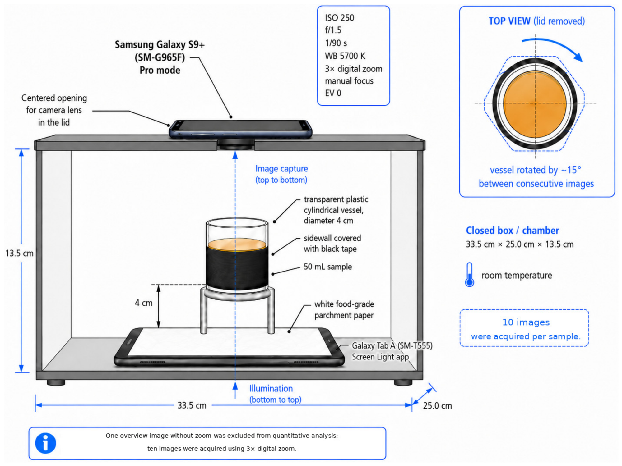
Digital images were acquired in a closed imaging chamber constructed from a box with dimensions of 33.5 × 25.0 × 13.5 cm. A Samsung Galaxy Tab A tablet (SM-T555; Samsung Electronics Co., Ltd., Suwon, Republic of Korea) was fixed centrally to the bottom of the chamber and used as the transmitted-light source. The Screen Light application, version 1.3.2 (JK.Fantasy; developer Sheng Wen Liao, Hsinchu City, Taiwan) was set to a uniform white background at maximum screen brightness. A sheet of white food-grade parchment paper was placed directly over the tablet screen to diffuse the emitted light, homogenize the illuminated field, and prevent the tablet pixel matrix from being visibly reproduced in images acquired using 3× digital zoom. The box remained closed during image acquisition to limit interference from ambient illumination.

The entire prepared solution (50 mL) was transferred to a transparent cylindrical plastic measurement vessel with an internal diameter of 4 cm. Because the same solution volume and vessel geometry were used for every sample, the liquid-column height was constant across the series. The lateral wall was covered with opaque black tape to reduce lateral illumination and reflections. The vessel was positioned on a dedicated holder with its base 4 cm above the tablet surface. A viewing aperture was made in the chamber lid, and the smartphone was positioned so that the camera lens was aligned with the center of the sample.

Images were recorded with a Samsung SM-G965F smartphone (Samsung Electronics Co., Ltd., Suwon, Republic of Korea) using the camera application in Pro mode. The acquisition parameters were fixed at ISO 250, an aperture of f/1.5, a shutter time of 1/90 s, and a white-balance setting of 5700 K. Exposure compensation was maintained at 0 EV. The image-adjustment controls for tint, contrast, saturation, highlights, and shadows were all set to 0, corresponding to the factory-default values. Manual focus (MF) was set at the second tick mark on the camera application’s unitless scale; no physical unit was displayed for this scale. For each concentration, one overview photograph was first acquired without digital zoom for documentation and excluded from quantitative analysis. Ten photographs of the samples were then captured using a 3× digital zoom setting. After each acquisition, the vessel was rotated by approximately 15° while all other geometrical and camera settings were kept unchanged. The images had a resolution of 3024 × 3024 pixels and were stored as RGB JPEG files. All measurements were performed at room temperature. A schematic representation of the acquisition chamber, illumination geometry, sample positioning, and smartphone alignment is provided in Figure 1.

2.3. Image Selection, Masking, and Region of Interest

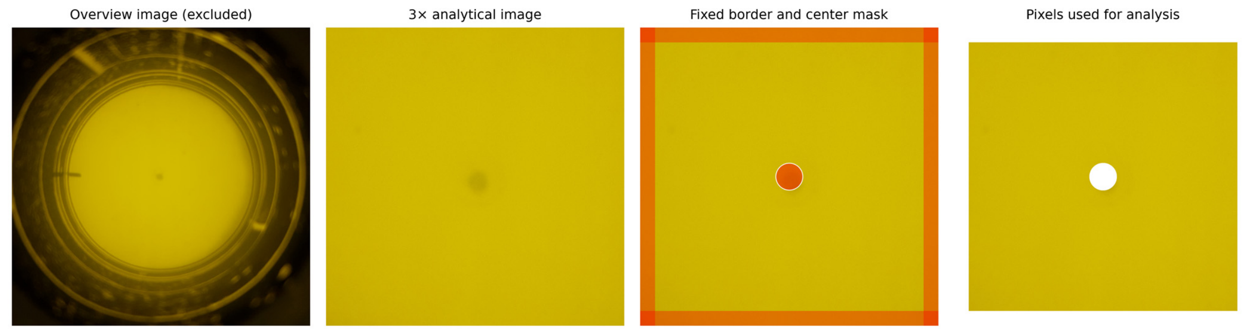
The 110 magnified images were included in the dataset. Each image was subjected to an identical deterministic mask as shown in Figure 2. First, a 150-pixel border was excluded to reduce the influence of edge darkening and residual vessel boundaries. Second, a circular region with a radius of 140 pixels centered on the image was excluded because it contained a factory-made center mark in the vessel. The mark was unrelated to the optical properties of honey and could otherwise introduce an artificial population of darker pixels. No concentration-dependent or manually adjusted segmentation was applied.

2.4. RGB Histogram Construction and Statistical Descriptors

For each retained image region, separate 256-bin histograms were calculated for the R, G, and B channels. For channel $c$, the normalized histogram probability $p_c\left(i\right)$ at intensity level $i$ satisfied Equation (1). The channel mean, variance, standard deviation, entropy, and energy were calculated according to Equations (2), (3), (4), (5) and (6), respectively, where $c$ ∈ {R, G, B} and $i$ ∈ {0, …, 255}. Terms with $p_c\left(i\right)=0$ were omitted from the entropy summation. Entropy followed Shannon’s definition, whereas skewness and excess kurtosis used bias-corrected sample formulas [58,59].

$${\displaystyle \sum _{i=0}^{255}}{p}_c\left(i\right)=1$$

(1)

$${\mu }_c={\displaystyle \sum _{i=0}^{255}}i\hspace{0.17em}{p}_c\left(i\right)$$

(2)

$${\sigma }_c^2={\displaystyle \sum _{i=0}^{255}}{\left(i-{\mu }_c\right)}^2{p}_c\left(i\right)$$

(3)

$${\sigma }_c=\sqrt{{\sigma }_c^2}$$

(4)

$$H_c=-{\displaystyle \sum _{\begin{array}{c}i=0\\ p_c\left(i\right)>0\end{array}}^{255}}{p}_c\left(i\right){\mathrm{l}\mathrm{o}\mathrm{g}}_2{p}_c\left(i\right)$$

(5)

$$E_c={\displaystyle \sum _{i=0}^{255}}{p}_c{\left(i\right)}^2$$

(6)

The complete candidate pool contained 102 descriptors organized into five families: location and percentiles, dispersion and width, distribution shape, information and peak structure, and inter-channel descriptors. The composition of the candidate pool is summarized in

Table 2. Summary of the 102 candidate descriptors extracted from whole-image RGB histograms.

Family	Included Descriptors	Analytical Purpose	n
Location and percentiles	Per channel: mean, median (P50), mode, P1, P5, P10, P25, P75, P90, P95, and P99	Location and shift of the intensity distribution	33
Dispersion and width	Per channel: variance, standard deviation, IQR, P95−P5 width, P99−P1 width, and FWHM	Within-image variability and histogram spread	18
Distribution shape	Per channel: skewness and excess kurtosis	Asymmetry and tail/peak shape	6
Information and peak	Per channel: entropy, energy, and dominant-peak height	Distribution concentration and peak prominence	9
Inter-channel	Ratios and differences for mean, median, mode, P10, P25, P75, and P90; six unstable B-denominator ratios excluded	Relative color balance between R, G, and B	36
Total candidate pool	Complete set entering the nested feature-selection workflow	Candidate predictors before fold-specific selection	102

. This grouping was used both for interpretation and for feature-family ablation experiments. Ratios with a blue-channel denominator were regularized using a small numerical constant to prevent division by zero. Because B_mode, B_p10, and B_p25 were frequently zero at low adulterant levels, the six corresponding R/B and G/B ratios were excluded from the candidate pool. Blue-channel ratios and shape descriptors were therefore interpreted cautiously and were not considered independently conclusive.

A total of 102 candidate descriptors entered the nested modeling workflow. Predictor ranking and subset size (5, 10, 20, 40, or all 102 descriptors) were determined exclusively within each inner cross-validation loop. Therefore, the models were not forced to use the full set and the withheld outer-test concentration did not contribute to feature selection. Complete feature names, mathematical definitions, units, and family assignments are provided in Supplementary Table S2.

2.5. Whole-Image and Random Patch Representations

Whole-image histograms were used as the primary representation because the imaged liquid region was nearly homogeneous and whole-image aggregation was expected to reduce pixel-level noise. Five non-overlapping 30 × 30-pixel patches were nevertheless extracted from each image as a planned methodological comparison with the earlier patch-oriented workflow reported by Wójcik et al. [50], yielding 550 technical subsamples. The earlier study used a separately prepared sample series following the same preparation scheme. The present comparison tested whether local sampling remained advantageous under fixed white-light illumination, locked camera settings, and the same deterministic exclusion criteria used for whole images; it was not intended to create additional independent experimental units. Patch coordinates were generated deterministically with a fixed seed.

The five patches extracted from each image remained linked to that image, and all images originating from the same concentration-specific preparation remained in the same outer fold. Patch predictions were first averaged at the image level and then at the concentration level before performance metrics were calculated. This hierarchical procedure prevented patches and images derived from the same physical preparation from being treated as independent test observations.

2.6. Descriptor Usefulness and Orientation-Level Technical Repeatability

Descriptor usefulness was evaluated at the concentration level. For each feature, the ten rotated technical images were summarized by their mean and standard deviation. Monotonic association with nominal syrup addition was quantified using Spearman’s rank correlation coefficient ρ_S. Technical repeatability across sample orientations was summarized by the median coefficient of variation and ICC(1,1) [60]. Signal separation was expressed as the ratio S_B/W between the standard deviation of the concentration-level means and the pooled within-level standard deviation. The transparent descriptive score used in Section 3.3 was defined as follows:

$$\mathrm{U}\mathrm{t}\mathrm{i}\mathrm{l}\mathrm{i}\mathrm{t}\mathrm{y}\left(j\right)=\left|{\rho }_S\left(j\right)\right|\times \mathrm{l}\mathrm{n}\left[1+S_{B/W}\left(j\right)\right]\times \mathrm{I}\mathrm{C}\mathrm{C}\left(1,1\right)\left(j\right)$$

(7)

The logarithm in Equation (7) limits domination by extremely large signal-to-within ratios; no min–max normalization or fitted weighting coefficients were used. The utility score was used only to order descriptive responses and was not interpreted as an independent feature contribution. A descriptor was considered promising when it combined a stable concentration trend with low orientation variability and when its predictive value was supported by nested modeling, restricted-feature analysis, or explainability results. Because many neighboring percentiles were strongly correlated, interpretation emphasized descriptor families and repeated patterns rather than isolated causal effects.

2.7. Regression Models

Five regression approaches were compared. Partial least-squares regression (PLSR) represented a supervised linear latent-component method appropriate for collinear predictors; unlike principal component analysis, PLSR constructs components using covariance with the response [61,62]. Support vector regression (SVR) was evaluated with linear and radial-basis-function (RBF) kernels. Random forest (RF), gradient boosting (GB), and extreme gradient boosting (XGBoost) represented nonlinear tree ensembles with distinct bagging, sequential boosting, and regularization strategies [63,64,65,66,67].

Candidate feature subsets for PLSR and SVR contained 5, 10, 20, 40, or all 102 descriptors. PLSR evaluated one to six latent components. SVR evaluated linear and radial-basis-function kernels over the predefined C, epsilon, and gamma values. The tree-ensemble search used deterministic candidate profiles spanning ensemble size, feature-subset size, tree depth, leaf or child constraints, regularization, and row and feature subsampling. Each outer fold evaluated 16 random forest, 15 gradient boosting, and 16 XGBoost profiles in every inner split. All candidates were evaluated exclusively within the inner training partitions of the nested design; the withheld outer concentration remained inaccessible until the selected pipeline had been refitted on the complete outer-training partition. When mean inner RMSE values differed by no more than 0.01 percentage point, the predefined tie rule favored fewer descriptors, shallower depth, stronger regularization, and then fewer trees. Complete candidate definitions and scores are archived in the reproducibility package.

2.8. Group-Aware Validation and Performance Metrics

The ten images of one concentration were never divided between training and test subsets because they were repeated photographs of one physical preparation. The outer loop left out one complete concentration-specific preparation at a time and repeated the procedure for all 11 levels. Within each outer training set, five deterministic inner folds held out paired low- and high-concentration levels. Variance filtering, univariate ranking, feature selection, scaling, and estimator fitting used only the corresponding inner-training data. The candidate with the lowest mean inner RMSE was selected and refitted on the complete outer-training partition before prediction of the ten images from the omitted concentration. This fully nested concentration-grouped design prevented replicate leakage and separated model selection from outer evaluation [52,53,54,55,56,68,69].

For each outer fold, the ten image predictions were averaged to obtain one concentration-level estimate. RMSE_nested-LOCO, MAE_nested-LOCO, and R²_nested-LOCO were calculated once from the eleven outer concentration-level predictions using Equations (8)–(10) [70]. Descriptive 95% nonparametric bootstrap intervals were calculated from these eleven outer predictions. Concentration-level residuals and SD_orientation values are reported in Supplementary Table S4. SD_orientation is the standard deviation among the ten rotated images of the same physical preparation and is not an uncertainty estimate for independently prepared samples. Residual predictive deviation (RPD_nested-LOCO) was calculated as RPD_nested-LOCO = s_y/RMSE_nested-LOCO, where s_y is the sample standard deviation of the eleven nominal reference levels.

$$\mathrm{R}\mathrm{M}\mathrm{S}\mathrm{E}=\sqrt{{\displaystyle \frac{1}{N}}{\displaystyle \sum _{j=1}^N}{\left(y_j-{\widehat{y}}_j\right)}^2}$$

(8)

$$\mathrm{M}\mathrm{A}\mathrm{E}={\displaystyle \frac{1}{N}}{\displaystyle \sum _{j=1}^N}\left|y_j-{\widehat{y}}_j\right|$$

(9)

$$R^2=1-{\displaystyle \frac{{\displaystyle {\sum }_{j=1}^N}{\left(y_j-{\widehat{y}}_j\right)}^2}{{\displaystyle {\sum }_{j=1}^N}{\left(y_j-\bar{y}\right)}^2}}$$

(10)

Here, N denotes the number of evaluated concentration levels, $y_j$ is the nominal gravimetric addition level, ${\widehat{y}}_j$ is the corresponding outer concentration-level prediction, and $\widehat{y}$is the mean reference level. Overall metrics used N = 11, whereas RMSE_{nested-LOCO,5–45} used the nine internal levels from 5% to 45%. The independent evaluation unit was therefore the concentration-specific preparation, not an individual image or patch.

Four quantities were kept distinct throughout the manuscript: prediction error (RMSE_nested-LOCO and MAE_nested-LOCO), orientation variability (SD_orientation and orientation range), the resolution-based uncertainty of the nominal gravimetric preparation, and sample-preparation variability. The last quantity could not be estimated because only one physical mixture was prepared per level. Nested LOCO evaluates a withheld level within the prepared series; it does not measure performance on a newly and independently prepared mixture or on a broader honey population.

After nested performance estimation, a final all-data refit was created for each algorithm. Candidate configurations were compared by concentration-wise selection cross-validation on the complete series, and the selected pipeline was fitted to all 110 images. RMSE_selection-CV was used solely for selecting the archived configuration. It is not an independent performance estimate and does not replace RMSE_nested-LOCO reported in Section 3.4.

2.9. Restricted-Feature Reference Model Design

To determine whether the broader multidescriptor representation provided improved predictive performance relative to simpler color summaries, four feature representations were compared: (i) an ordinary least squares (OLS) model using G_mean as the sole predictor; (ii) the complete set of 22 direct G-channel descriptors; (iii) the three channel means R_mean, G_mean, and B_mean; and (iv) models derived from the full candidate pool of 102 descriptors. For the three multivariable representations, PLSR, SVR, RF, GB, and XGBoost were tuned using the same concentration-grouped validation logic as in the primary analysis. Feature ranking, subset selection, scaling, and hyperparameter selection were repeated within the corresponding training partitions to avoid information leakage. The predefined G_mean OLS model involved no feature selection or hyperparameter tuning.

Nested-LOCO metrics were used to compare the predictive performance of the four feature representations, whereas RMSE_selection-CV was used only to identify the final all-data configuration within each multivariable representation. Thus, RMSE_selection-CV was not treated as an independent estimate of predictive performance.

A pixelwise sRGB-to-CIELAB analysis was not reconstructed from channel means because such a transformation would be mathematically invalid. The RGB-to-CIELAB transformation is nonlinear and must be applied to the original pixel-level RGB values using a defined colorimetric conversion and reference white; CIELAB descriptors therefore cannot be obtained by transforming summary RGB means. A direct pixel-level CIELAB analysis is consequently identified as a separate future comparison rather than approximated from the available RGB summary descriptors.

2.10. Explainable Artificial Intelligence and Descriptor-Family Analysis

One final all-data model was selected and refitted for each of the five algorithms after nested performance estimation. For descriptor j and method m, the mean absolute SHAP importance, within-method normalized importance, performance-derived method weight, and the performance-weighted cross-model score were defined by Equations (11), (12), (13) and (14), respectively:

$$A_{jm}={\displaystyle \frac{1}{110}}{\displaystyle \sum _{i=1}^{110}}\left|{\varphi }_{ijm}\right|$$

(11)

$$S_{jm}={\displaystyle \frac{A_{jm}}{{\displaystyle {\sum }_{l=1}^{p_m}}{A}_{lm}}}$$

(12)

$$w_m={\displaystyle \frac{{\mathrm{R}\mathrm{M}\mathrm{S}\mathrm{E}}_{\mathrm{n}\mathrm{e}\mathrm{s}\mathrm{t}\mathrm{e}\mathrm{d}\text{-}\mathrm{L}\mathrm{O}\mathrm{C}\mathrm{O},m}^{-2}}{{\displaystyle {\sum }_{l=1}^5}{\mathrm{R}\mathrm{M}\mathrm{S}\mathrm{E}}_{\mathrm{n}\mathrm{e}\mathrm{s}\mathrm{t}\mathrm{e}\mathrm{d}\text{-}\mathrm{L}\mathrm{O}\mathrm{C}\mathrm{O},l}^{-2}}}$$

(13)

$$C_j={\displaystyle \sum _{m=1}^5}{w}_m{S}_{jm}$$

(14)

Here, φ_ijm denotes the SHAP value for image i, descriptor j, and method m, and p_m the number of descriptors retained in the final model for method m, RMSE_{nested-LOCO,m} is RMSE_nested-LOCO for method m. In Equation (13), the index l runs over the five regression methods in the normalization sum. PLSR and linear SVR were decomposed exactly in their transformed linear coordinate systems, whereas interventional TreeSHAP was applied for random forest, gradient boosting, and XGBoost with the 110 transformed observations as the empirical background dataset [71,72]. Fold-wise descriptor inclusion frequency and SHAP-effect direction were reported separately and were not incorporated into C_j. VIP, permutation importance, descriptor-family ablation, and the restricted-feature comparisons were retained as independent corroborating analyses [73,74]. SHAP and the other importance measures describe how fitted models distribute predictive information; they do not establish independent or causal effects for highly correlated variables [57,75]. Descriptor-family ablation re-evaluated PLSR and SVR using location/percentile, dispersion/width, shape, information/peak, and inter-channel descriptors under the same nested LOCO structure.

2.11. Software and Reproducibility

Image decoding, descriptor extraction, descriptive analyses, explainability summaries, and figure generation were performed in Python 3.13.5 on Linux x86_64. This environment used NumPy 2.3.5, pandas 2.2.3, SciPy 1.17.0, Pillow 12.2.0, OpenCV 4.13.0, scikit-image 0.26.0, SHAP 0.50.0, and Matplotlib 3.10.8 [76,77,78,79,80]. The audited whole-image and patch nested-model outputs and the final serialized refits were regenerated from the canonical feature tables in Python 3.12.13 using NumPy 2.5.1, pandas 2.2.3, SciPy 1.18.0, joblib 1.5.3, scikit-learn 1.8.0, and XGBoost 3.1.3. Separate exact environment locks and run manifests are archived. A fixed modeling seed of 20260720 was used for stochastic estimators, and a separate seed of 20260721 was used for deterministic patch sampling and repeated permutation procedures. Whole-image JPEGs were decoded using OpenCV, whereas the historical patch-table extraction used Pillow. The fixed whole-image mask retained 7,358,187 pixels and used Pillow’s inclusive filled-ellipse rasterization for the central exclusion. Histogram FWHM was measured in intensity-bin units; exact boundary conventions are supplied with the executable descriptor code.

The reproducibility package contains processed whole-image and patch feature tables, group identifiers, deterministic patch coordinates, fixed masks, model-search configurations, every candidate score, fold-wise selected features and hyperparameters, out-of-fold predictions, final refitted model objects, executable analysis scripts, environment locks, checksums, manuscript-ready tables, and figure files. These materials are available at https://github.com/GosiaDz/honey-main-files (accessed on 14 August 2026). The standardized raw-JPEG archive and image inventory are available separately at https://github.com/GosiaDz/honey-images (accessed on 14 August 2026).

3. Results

3.1. Image-Set Verification and Technical Repeatability

The archive contained 121 images: 11 concentration levels with 11 files per level. For every concentration, the unzoomed overview image, standardized in the repository as Dxx_overview.jpg, showed the complete vessel and was excluded. The remaining ten images acquired using 3× digital zoom yielded the intended analytical set of 110 images. All photographs had identical dimensions (3024 × 3024 pixels), and no byte-identical duplicate images were detected.

The color field was visually homogeneous, with a small central vessel mark and mild edge darkening. Applying the fixed mask removed these non-sample structures without concentration-dependent adjustment. Technical repeatability was high for mean channel intensity. Across concentration levels, the median coefficients of variation were approximately 0.05% for R, 0.08% for G, and 0.77% for B. The larger relative variability of B partly reflected its very low absolute intensity at the lowest addition levels.

3.2. Evolution of RGB Distributions with Syrup Addition

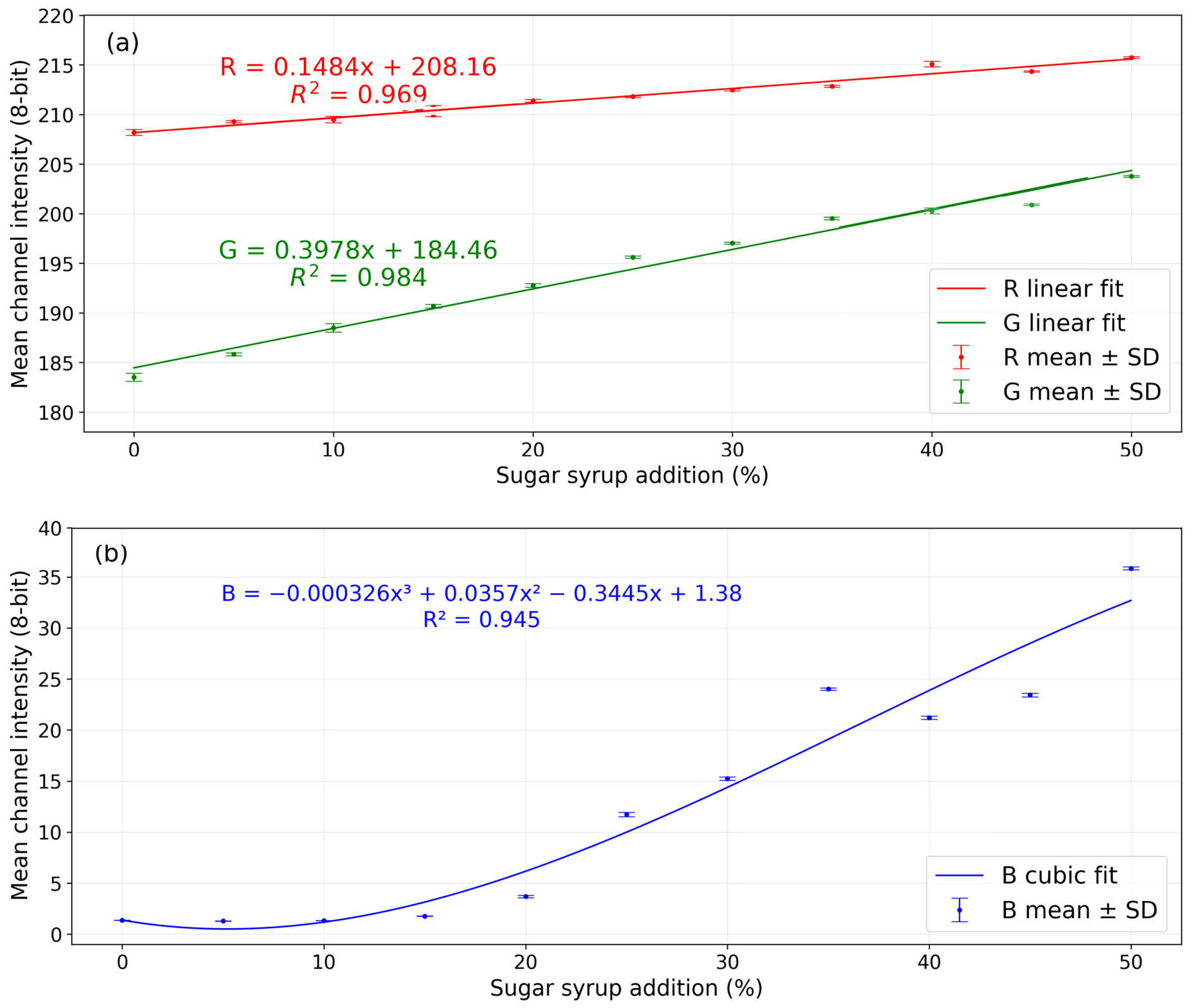
The mean R and G intensities increased across the concentration series, whereas B showed a low-intensity plateau followed by a strong, non-linear rise from approximately 20–25% sugar syrup addition onward. Mean G increased from 183.52 at 0% to 203.76 at 50%, mean R increased from 208.19 to 215.74, and mean B increased from 1.37 to 35.85. To visualize these univariate responses, least-squares trend models were fitted to the concentration-level means (Figure 3). Linear models described the R- and G-channel responses with R² values of 0.969 and 0.984, respectively, whereas an illustrative cubic polynomial was used for the B channel (R² = 0.945). These curves are descriptive trend fits and are distinct from the multivariate predictive models evaluated in Section 3.4. At low concentration levels, approximately one-third or more of valid pixels were recorded at B = 0, indicating channel clipping; consequently, B-based effects were interpreted cautiously.

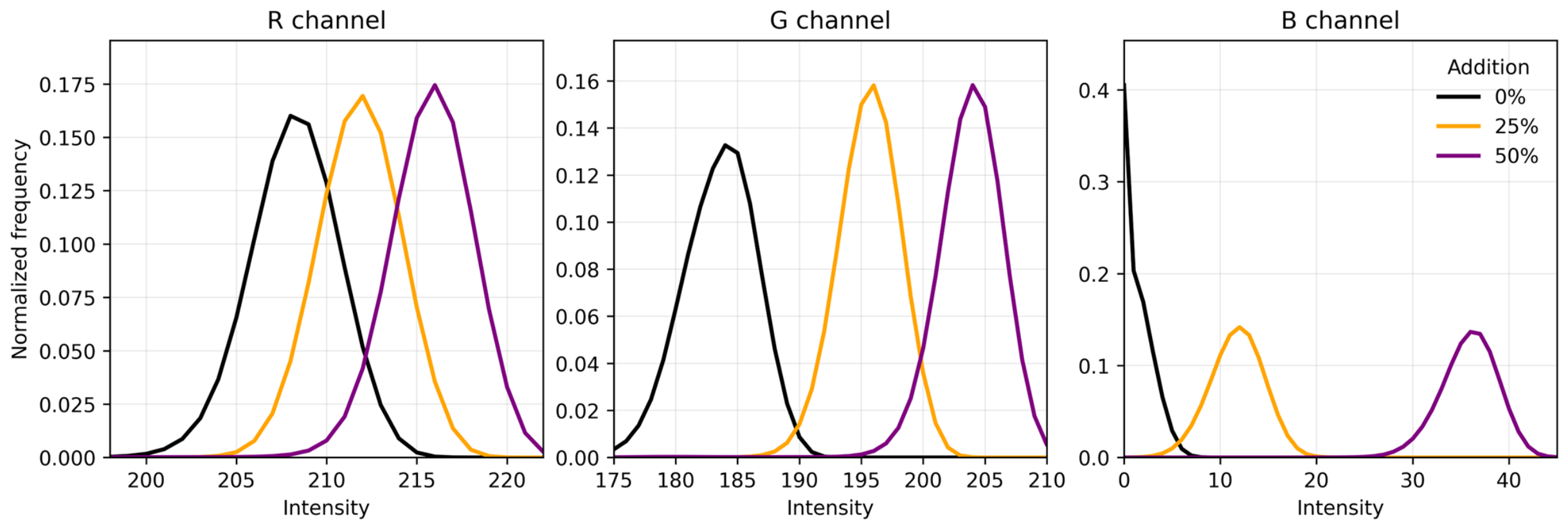
Histogram shifts were most regular in the G channel. The fitted G-channel slope (0.3978 intensity units per percentage point) was approximately 2.7 times as large as the corresponding R-channel slope (0.1484), indicating a stronger green-channel response over the investigated concentration range. The concentration-level means of G_mean and G_p95 were strictly monotonic in the present dataset (Spearman ρ = 1.000). R-channel location descriptors also showed strong monotonic relationships, whereas the B-channel response remained non-linear and exhibited local deviations from the fitted cubic trend, particularly between 35% and 45% syrup addition. This further supports the interpretation of the curves in Figure 3 as descriptive visualizations rather than calibration models. Distribution-shape and dispersion features were generally less consistent. Overall, the histograms showed that the dominant image-derived response was a shift in the location of the intensity distribution rather than a large broadening or restructuring of the narrow color distribution.

Table 3. Concentration-level R-channel descriptors averaged across ten technical images. Histogram width was defined as P95−P5; ΔMean denotes the shift in channel mean relative to the 0% reference sample.

Adulterant (%)	Mean	Median	SD	Skew.	Kurt.	Entropy	Energy	Width	Peak Position	ΔMean vs. 0%
0	208.19	208.30	2.50	−0.280	0.644	3.358	0.114	8.10	208.50	0.00
5	209.28	209.00	2.53	−0.701	4.195	3.334	0.117	7.80	209.00	1.09
10	209.50	209.60	2.42	−0.209	0.353	3.312	0.118	7.80	209.60	1.30
15	209.95	210.00	2.35	−0.311	1.672	3.259	0.122	7.90	210.00	1.75
20	211.38	211.30	2.45	−0.515	2.994	3.306	0.118	7.60	211.60	3.19
25	211.81	212.00	2.36	−0.279	1.318	3.268	0.121	7.80	212.00	3.61
30	212.49	212.80	2.39	−0.433	2.212	3.282	0.120	7.20	212.90	4.29
35	212.83	213.00	2.32	−0.447	2.565	3.236	0.124	7.50	213.00	4.64
40	215.08	215.10	2.47	−0.871	5.942	3.295	0.120	7.80	215.20	6.89
45	214.34	214.30	2.51	−1.453	11.147	3.264	0.123	7.20	214.60	6.15
50	215.74	216.00	2.61	−2.001	16.166	3.278	0.123	7.40	216.00	7.55

,

Table 4. Concentration-level G-channel descriptors averaged across ten technical images. Histogram width was defined as P95−P5; ΔMean denotes the shift in channel mean relative to the 0% reference sample.

Adulterant (%)	Mean	Median	SD	Skew.	Kurt.	Entropy	Energy	Width	Peak Position	ΔMean vs. 0%
0	183.52	183.70	2.96	−0.341	0.213	3.596	0.096	9.60	184.50	0.00
5	185.83	186.00	2.88	−0.670	2.280	3.530	0.103	9.20	186.10	2.31
10	188.50	188.70	2.69	−0.358	0.490	3.454	0.108	8.90	188.90	4.98
15	190.68	190.90	2.59	−0.519	1.614	3.389	0.113	8.60	191.00	7.16
20	192.78	193.00	2.68	−0.473	2.099	3.441	0.108	8.60	193.00	9.25
25	195.62	195.90	2.54	−0.350	1.111	3.378	0.112	8.50	196.00	12.10
30	197.03	197.00	2.64	−0.435	1.587	3.425	0.109	8.20	197.00	13.50
35	199.52	199.90	2.48	−0.538	2.456	3.327	0.117	7.50	200.00	16.00
40	200.29	200.50	2.56	−0.830	4.970	3.347	0.116	7.70	200.70	16.77
45	200.90	201.00	2.71	−1.372	9.322	3.379	0.114	8.20	201.00	17.38
50	203.76	204.00	2.84	−1.724	12.335	3.418	0.112	8.70	204.00	20.24

and

Table 5. Concentration-level B-channel descriptors averaged across ten technical images. Histogram width was defined as P95−P5; ΔMean denotes the shift in channel mean relative to the 0% reference sample.

Adulterant (%)	Mean	Median	SD	Skew.	Kurt.	Entropy	Energy	Width	Peak Position	ΔMean vs. 0%
0	1.37	1.00	1.51	1.012	0.385	2.282	0.253	4.00	0.00	0.00
5	1.29	1.00	1.47	1.066	0.518	2.223	0.266	4.00	0.00	−0.08
10	1.34	1.00	1.50	1.029	0.410	2.257	0.259	4.00	0.00	−0.03
15	1.76	1.10	1.67	0.758	−0.129	2.521	0.201	5.00	0.00	0.39
20	3.69	3.80	2.36	0.361	−0.322	3.201	0.119	8.00	3.30	2.32
25	11.73	12.00	2.81	−0.161	−0.004	3.535	0.100	9.20	12.00	10.36
30	15.24	15.10	2.98	−0.113	−0.072	3.622	0.094	10.00	15.30	13.87
35	24.02	24.00	2.83	−0.260	0.080	3.538	0.100	9.40	24.40	22.65
40	21.22	21.20	2.98	−0.211	0.085	3.614	0.095	10.00	21.70	19.85
45	23.44	23.70	2.97	−0.206	−0.005	3.611	0.095	9.70	23.90	22.07
50	35.85	36.00	2.97	−0.363	0.342	3.602	0.097	9.20	36.40	34.47

summarize the principal R-, G-, and B-channel descriptors averaged across the ten 3× digital-zoom images at each concentration. The corresponding concentration-level normalized histograms are shown in Figure 4.

3.3. Usefulness and Stability of Statistical Descriptors

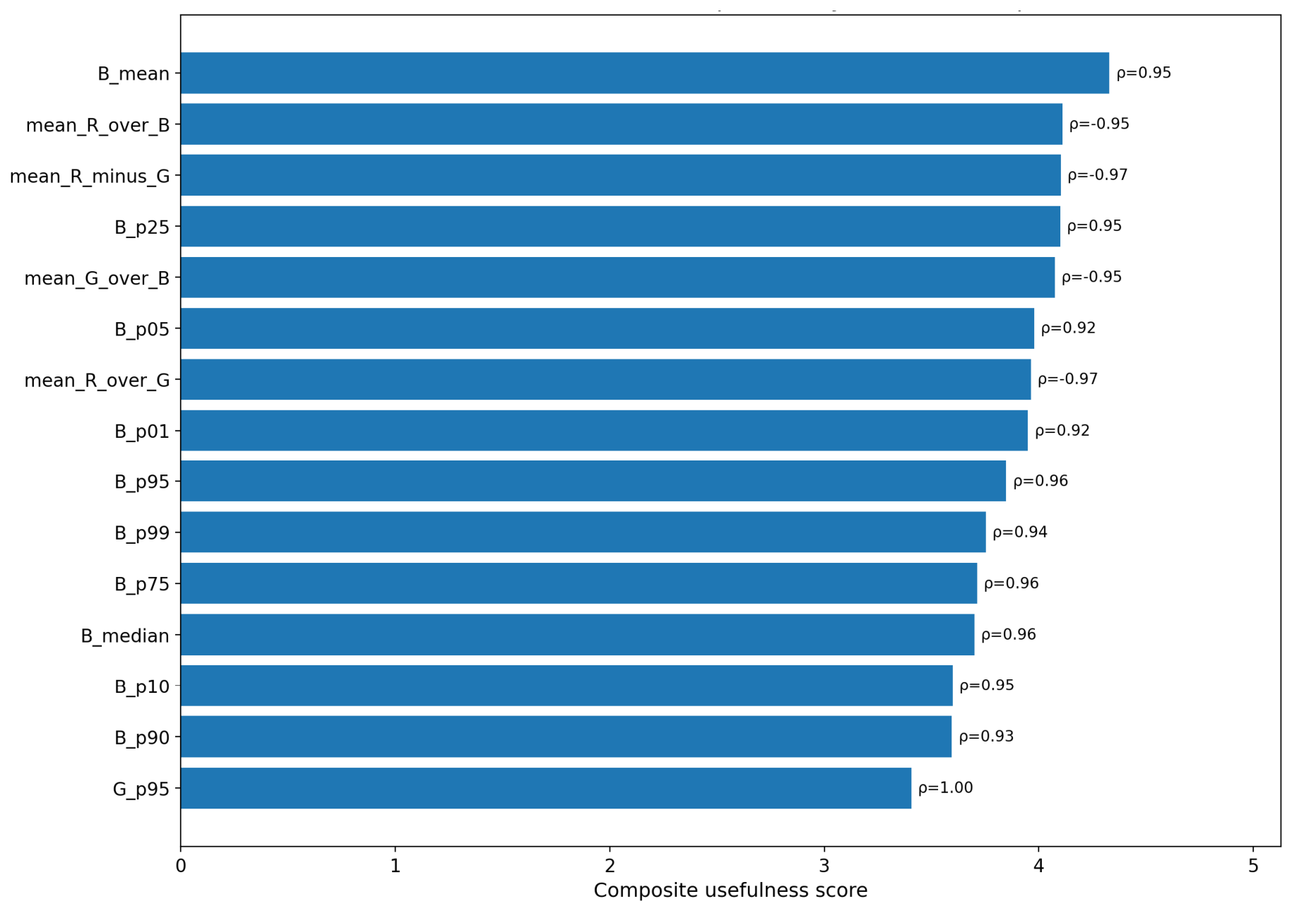
Feature usefulness depended on both effect magnitude and repeatability. Several B-channel location descriptors achieved very large between-to-within variability ratios because technical variability was small compared with the concentration-dependent increase. Mean B had Spearman correlation of ρ = 0.945, ICC (1,1) = 0.9999, and a between-to-within variability ratio of 96.5. The R−G mean difference and R/G mean ratio showed strong negative monotonic relationships (ρ = −0.973) and similarly high repeatability. G-channel location features exhibited perfect rank monotonicity and low coefficients of variation, making them particularly attractive from an interpretability perspective. Representative statistics are summarized in

Table 6. Representative descriptor usefulness and orientation-level technical-repeatability statistics.

Feature	Family	Spearman Correlation ρ	Pearson Correlation r	Median CV (%)	ICC(1,1)	Between/Within
Mean G	location percentiles	1.000	0.992	0.085	0.9988	29.2
P95 G	location percentiles	1.000	0.993	0.000	0.9988	29.2
Mean R	location percentiles	0.991	0.984	0.047	0.9944	13.4
Mean B	location percentiles	0.945	0.944	0.769	0.9999	96.5
P95 B	location percentiles	0.963	0.955	0.000	0.9996	53.4
Mean(R−G)	interchannel	−0.973	−0.972	0.320	0.9998	67.0
Mean R/Mean G	interchannel	−0.973	−0.971	0.032	0.9997	57.9
Entropy B	information peak	0.845	0.899	0.742	0.9985	25.5
Entropy G	information peak	−0.718	−0.743	1.252	0.7384	1.7
SD R	dispersion width	0.118	0.171	3.348	0.3660	0.8

.

The transparent utility ranking combined absolute monotonic association, the log-transformed signal-to-within ratio, and ICC according to Equation (7). Location/percentile and selected inter-channel descriptors occupied the highest positions. The score is descriptive: it does not quantify an independent predictive contribution of each descriptor. The logarithmic transformation reduces the disproportionate influence of very large ratios, particularly those observed for low-intensity B-channel descriptors. The resulting ranking is shown in Figure 5.

3.4. Nested Comparison of Regression Methods

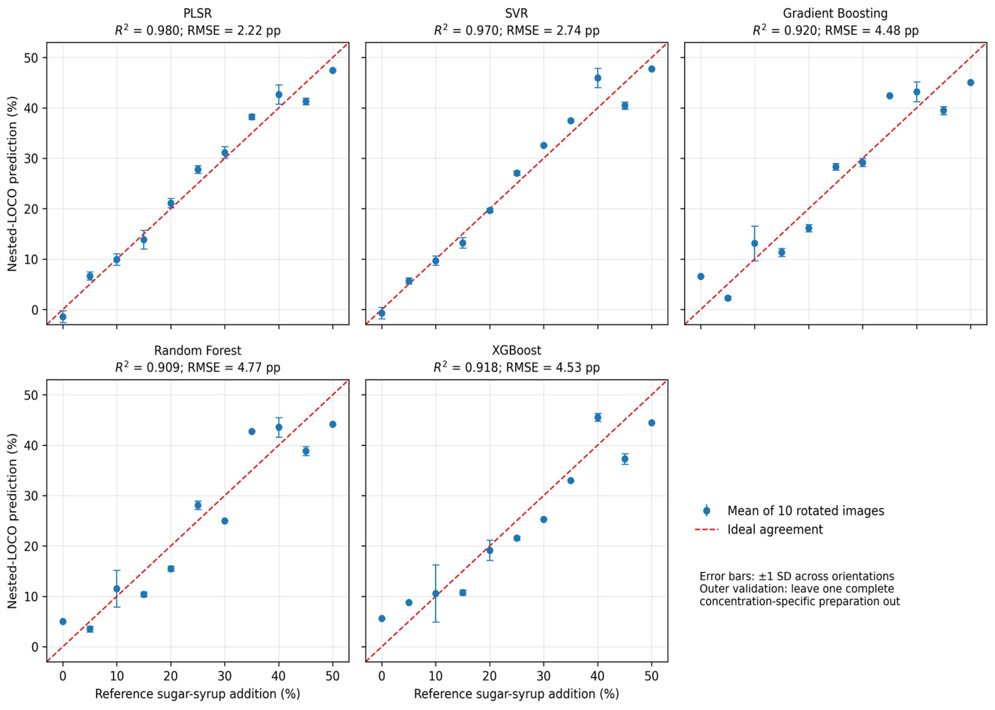
Under nested leave-one-concentration-out validation, PLSR achieved the lowest prediction error among the primary full-feature models, with RMSE_nested-LOCO = 2.22 percentage points and R²_nested-LOCO = 0.980; SVR ranked second. Both methods outperformed the three tree ensembles (

Table 7. Concentration-level performance under nested leave-one-concentration-out cross-validation.

Model	R2nested-LOCO	RMSEnested-LOCO (pp)	95% Bootstrap CI	MAEnested-LOCO (pp)	RMSEnested-LOCO,5–45 (pp)	SDorientation (pp)	Max Orientation Range (pp)	RPDnested-LOCO
PLSR	0.980	2.22	1.60–2.76	1.96	2.25	1.01	5.06	7.47
SVR	0.970	2.74	1.54–3.80	2.16	2.93	0.70	4.64	6.05
GB	0.920	4.48	3.39–5.48	4.11	4.13	0.88	8.35	3.70
XGBoost	0.918	4.53	3.36–5.56	4.01	4.25	0.94	13.79	3.66
RF	0.909	4.77	3.71–5.73	4.41	4.61	0.81	9.25	3.48

). Performance for the internal 5–45% range is reported separately to distinguish interpolation from boundary extrapolation. The 95% bootstrap intervals are descriptive because only 11 concentration-specific preparations were available. SD_orientation and maximum orientation range describe variability among rotated images of the same physical preparation and should not be interpreted as confidence intervals for prediction of new preparations. Concentration-level predictions are shown in Figure 6. The corresponding RPD_nested-LOCO values confirmed the same ranking: PLSR and SVR showed the strongest scale-relative predictive performance, while all three tree ensembles also achieved RPD_nested-LOCO above 3.

The mean SD_orientation values for PLSR and SVR were 1.01 and 0.70 percentage points, respectively, and their maximum orientation ranges were 5.06 and 4.64 percentage points. These metrics characterize prediction variability associated with vessel rotation within the same physical preparation. They should not be interpreted as standard errors, confidence intervals, or estimates of variability among independently prepared samples.

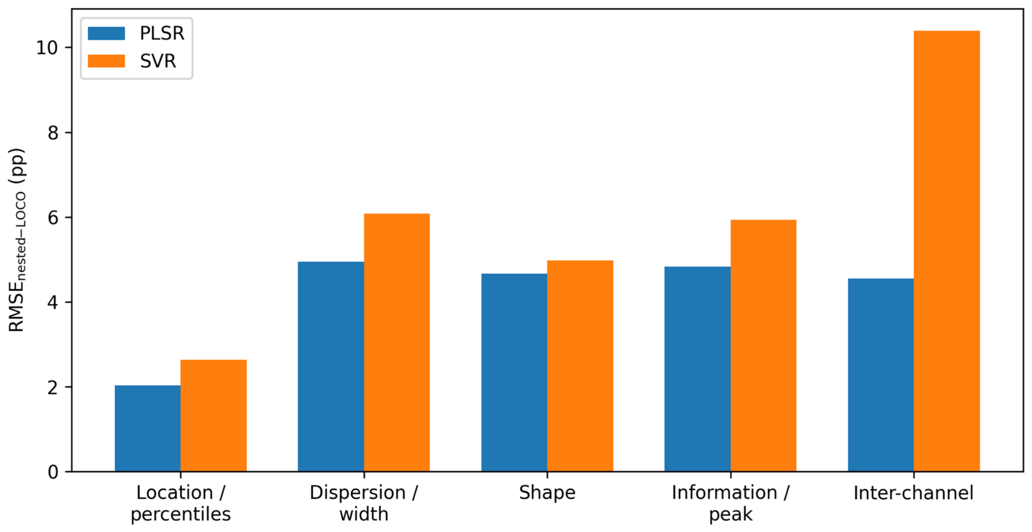
3.5. Feature-Family Ablation

Descriptor-family ablation was used to assess whether predictive information was concentrated in histogram location or distributed across the other descriptor families. PLSR and SVR were therefore re-evaluated using one family at a time under the same nested LOCO cross-validation. Location and percentile descriptors contained most of the usable predictive information. PLSR restricted to the 33 location/percentile descriptors achieved R²_nested-LOCO = 0.984, RMSE_nested-LOCO = 2.03, and MAE_nested-LOCO = 1.67 percentage points, slightly improving upon the full-feature PLSR model. The corresponding SVR achieved R²_nested-LOCO = 0.972 and RMSE_nested-LOCO = 2.64 pp. Models based only on dispersion/width, shape, information/peak, or inter-channel descriptors produced substantially larger errors. In particular, the inter-channel-only SVR was unstable (RMSE_nested-LOCO = 10.39 pp), demonstrating that ratios and differences were useful mainly in combination with direct channel-location variables rather than as an isolated representation. Numerical results and their graphical comparison are provided in

Table 8. Feature-family ablation results for PLSR and SVR.

Feature Family	Candidate Features	Model	R2nested-LOCO	RMSEnested-LOCO (pp)	MAEnested-LOCO (pp)
Location and percentiles	33	PLSR	0.984	2.03	1.67
		SVR	0.972	2.64	1.91
Dispersion and width	18	PLSR	0.902	4.95	3.86
		SVR	0.852	6.08	4.62
Distribution shape	6	PLSR	0.913	4.66	3.76
		SVR	0.901	4.98	4.15
Information and peak	9	PLSR	0.907	4.83	4.31
		SVR	0.860	5.93	4.42
Inter-channel	36	PLSR	0.917	4.55	3.86
		SVR	0.568	10.39	6.48

and Figure 7, respectively.

3.6. Restricted-Feature Reference Analyses

The restricted comparison was motivated by the feature-ranking and stability results. Several G-channel location descriptors occupied leading positions, were frequently selected, and showed stable concentration-dependent responses. The comparison therefore tested whether prediction was driven mainly by G_mean, by additional information in the full G-channel histogram, by the three RGB means, or by complementary descriptors selected from the broader candidate space.

Under fully nested LOCO evaluation, G-channel-only models achieved RMSE_nested-LOCO values of 1.67 pp for PLSR and 1.88 pp for SVR, compared with 2.25 and 1.99 pp for the corresponding RGB-mean models. The predefined G_mean ordinary least-squares reference achieved RMSE_nested-LOCO = 2.48 pp. These nested results show that the green-channel response carried strong predictive information and that a multidescriptor representation of its histogram provided useful information beyond that captured by G_mean alone. The restricted representations are reported as secondary sensitivity analyses and do not replace the prespecified primary full-feature comparison.

Table 9. Final configurations selected for the full and restricted feature representations.

Model	Rank Within Method	Feature Representation	Retained Descriptors	RMSEselection-CV (pp)
OLS	1	G_mean	1	2.230 *
SVR	1	Full descriptor pool	102 of 102	1.340
	2	G-channel descriptors	10 of 22	1.455
	3	RGB channel means	3	1.556
PLSR	1	G-channel descriptors	20 of 22	1.604
	2	Full descriptor pool	40 of 102	1.607
	3	RGB channel means	3	1.666
Random Forest	1	Full descriptor pool	40 of 102	3.562
	2	G-channel descriptors	5 of 22	4.207
	3	RGB channel means	3	4.302
Gradient Boosting	1	Full descriptor pool	40 of 102	3.630
	2	G-channel descriptors	22 of 22	3.902
	3	RGB channel means	3	4.005
XGBoost	1	G-channel descriptors	22 of 22	3.850
	2	RGB channel means	3	4.263
	3	Full descriptor pool	40 of 102	4.289

* For OLS, 2.230 pp is the concentration-grouped selection-CV error of the single predefined G_mean configuration; it is not RMSE_nested-LOCO.

summarizes the final configurations identified by full-dataset concentration-grouped selection cross-validation. RMSE_selection-CV is reported only for configuration selection and is not an independent test-performance estimate. Models selected from the full descriptor pool gave the lowest RMSE_selection-CV for SVR, RF, and GB; the restricted G-channel representation was marginally lower for PLSR and XGBoost. The predefined G_mean OLS reference involved no feature or hyperparameter search.

3.7. Performance-Weighted Explainability Analysis

The explainability analysis integrated all five final models rather than relying on SHAP values from gradient boosting alone. Method weights derived from RMSE_nested-LOCO were 42.40% for PLSR, 27.78% for SVR, 10.42% for gradient boosting, 9.19% for random forest, and 10.21% for XGBoost. The reconstruction error was below 2.3 × 10⁻⁵ for every implementation, confirming numerical consistency of the decomposition.

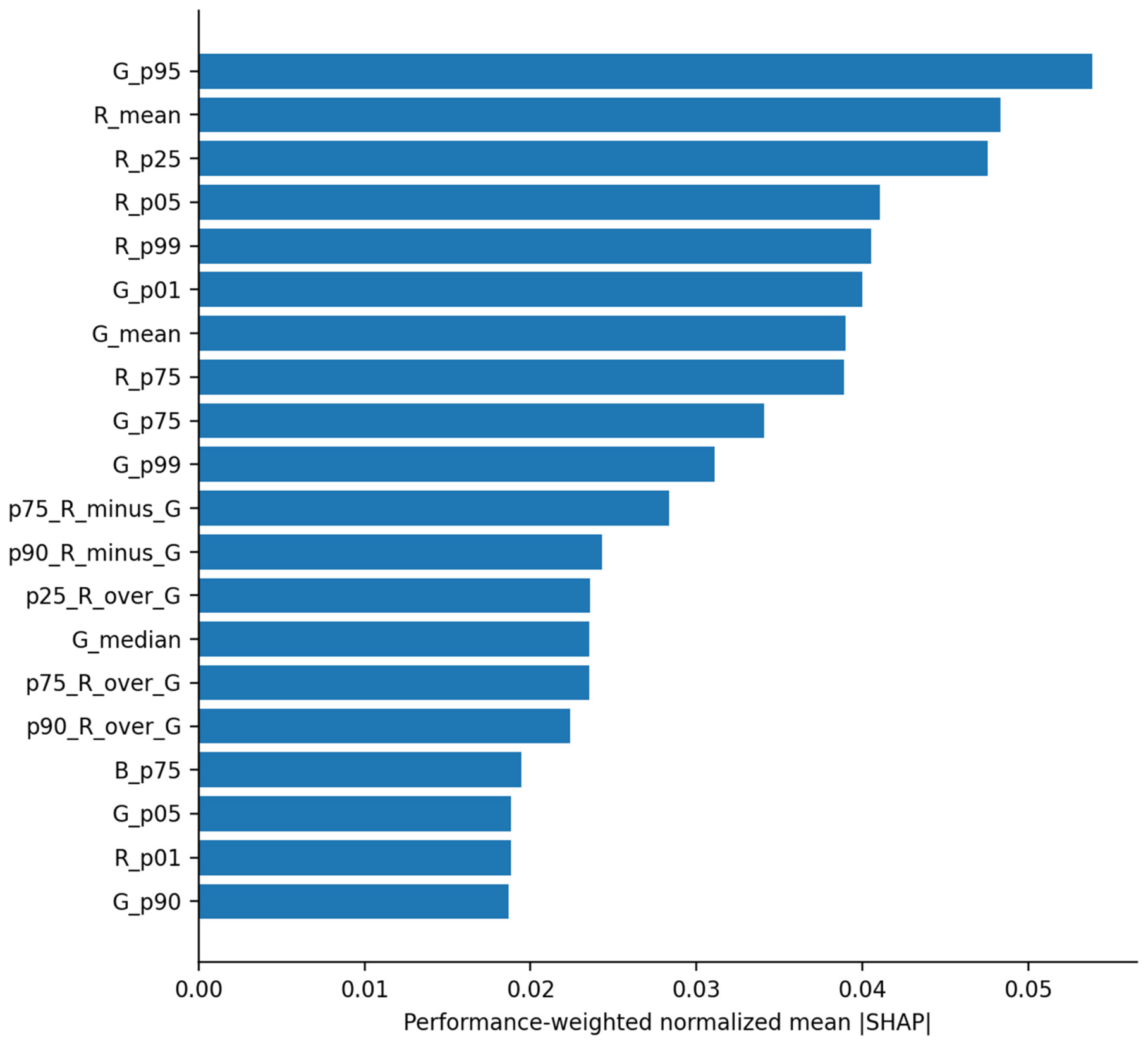
The performance-weighted SHAP consensus ranked G_p95, R_mean, R_p25, R_p05, and R_p99 highest. Location and percentile descriptors accounted for 67.7% of the total consensus score, followed by inter-channel descriptors at 27.2%; dispersion, shape, and information/peak families together contributed approximately 5%. Several leading location descriptors had the same positive direction across all five methods. Sign reversals for other neighboring percentiles are consistent with information sharing among correlated predictors and emphasize that an individual SHAP sign should not be interpreted as evidence of an independent chemical mechanism. Figure 8 presents the highest-ranked descriptors.

Selection stability was evaluated separately. G_mean, G_p75, G_p90, and G_p95 were included in 100% of outer models across all five methods, and G_mode reached 98.2%. The high stability of the G family explains the strong restricted-feature results, while the high SHAP ranks of several R descriptors show that the broader RGB space can provide complementary information in selected algorithms. VIP, permutation importance, and family ablation supported the dominant role of location variables but were not averaged into the SHAP score. Exact consensus scores, descriptor families, and model-specific effect directions are reported in Supplementary Table S6.

At nominal addition levels of 0–15%, 31–42% of valid image pixels had a blue-channel intensity of zero, indicating substantial lower-bound clipping. Six ratios with frequently zero B-channel descriptors in the denominator had already been excluded a priori. The remaining B-channel features were retained in the candidate pool but interpreted cautiously.

A post-hoc nested sensitivity analysis showed that excluding five clipping-sensitive B-channel shape/information descriptors changed RMSE_nested-LOCO only slightly, from 2.22 to 2.18 for PLSR and from 2.74 to 2.69 for SVR. Excluding all direct and derived B-related descriptors yielded RMSE_nested-LOCO values of 1.78 and 1.80, respectively. These results show that prediction did not depend on clipped B-channel structure; however, the no-B analysis was initiated after inspection of the data and is therefore reported as a diagnostic sensitivity analysis rather than as a newly selected primary model.

3.8. Whole-Image Versus Patch-Based Modeling

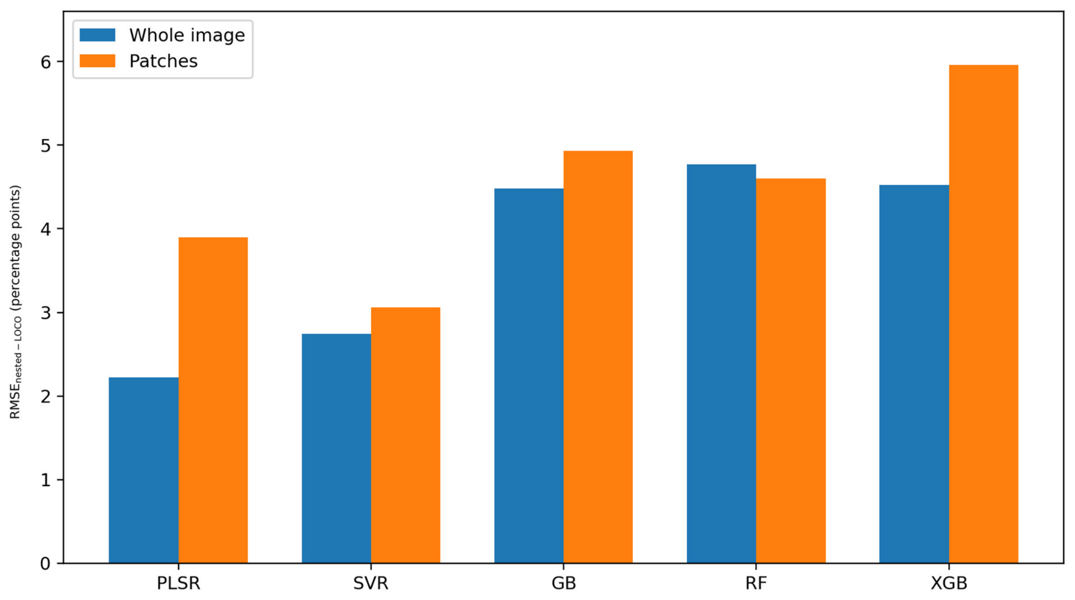
The patch analysis assessed whether local color summaries preserved predictive accuracy under the same concentration-grouped evaluation. The 550 patches remained technical subsamples of 11 physical preparations. Whole-image descriptors produced lower RMSE_nested-LOCO for PLSR, SVR, GB, and XGBoost in the matched representation comparison, whereas patch-based Random Forest improved modestly. Patch models also showed greater orientation variability. Under the present controlled acquisition protocol with fixed smartphone settings, local patch sampling therefore offered no general advantage over whole-image histograms. The numerical comparison is reported in

Table 10. Comparison of whole-image and patch-based performance under nested LOCO cross-validation. Errors and SD_orientation are expressed in percentage points of syrup addition.

Model	Whole R2nested-LOCO	Whole RMSEnested-LOCO (pp)	Whole MAEnested-LOCO (pp)	Patch R2nested-LOCO	Patch RMSEnested-LOCO (pp)	Patch MAEnested-LOCO (pp)	Patch SDorientation (pp)
PLSR	0.980	2.22	1.96	0.939	3.90	3.48	1.24
SVR	0.970	2.74	2.16	0.963	3.06	2.26	1.65
GB	0.920	4.48	4.11	0.903	4.93	3.96	1.48
RF	0.909	4.77	4.41	0.915	4.60	3.70	1.67
XGBoost	0.918	4.53	4.01	0.858	5.96	5.07	1.24

and visualized in Figure 9.

3.9. Final All-Data Model Refits

After nested performance estimation, one final whole-image model bundle per algorithm was selected and refitted to all 110 analytical images.

Table 11. Final whole-image all-data model configurations selected by concentration-grouped selection cross-validation and refitted to all 110 analytical images. RMSE_selection-CV was used only for configuration selection and is not an independent test-set estimate.

Model	Retained Descriptors	Final Selected Configuration	RMSE selection-CV (pp)
PLSR	40	6 latent components; scale = False after fold-local standardization	1.607
SVR	102	linear kernel; C = 0.1; epsilon = 0.1	1.340
RF	40	n_estimators = 300; max_depth = 8; min_samples_leaf = 3; max_features = 0.8	3.562
GB	40	n_estimators = 200; learning_rate = 0.05; max_depth = 3; min_samples_leaf = 2; subsample = 0.7	3.630
XGBoost	40	n_estimators = 300; learning_rate = 0.03; max_depth = 4; min_child_weight = 5; subsample = 0.7; colsample_bytree = 0.5; reg_lambda = 10; tree_method = hist; max_bin = 64	4.289

reports the best configuration among the predefined candidate profiles together with its RMSE_selection-CV. These values answer a configuration-selection question and are not independent performance estimates.

For the linear PLSR and SVR refits, each retained descriptor was standardized according to Equation (15), where x_j is the measured descriptor, μ_j and s_j are the all-data training mean and standard deviation, and z_j is the standardized value. Prediction then follows Equation (16), where p is the number of descriptors retained in the final model, w_j—the model coefficient for standardized descriptor, b₀—the intercept, $\widehat{y}$—the predicted syrup addition level. RF averages fitted regression trees as in Equation (17), where M the number of trees. GB and XGBoost follow the general additive form given in Equation (18), in which F₀ is the initial prediction, η is the learning rate, and h_m denotes the contribution of the tree added at boosting stage m.

$$z_j={\displaystyle \frac{x_j-{\mu }_j}{s_j}}$$

(15)

$$\widehat{y}=b_0+{\displaystyle \sum _{j=1}^p}{w}_j{z}_j$$

(16)

$${\widehat{y}}_{\mathrm{R}\mathrm{F}}\left(x\right)={\displaystyle \frac{1}{M}}{\displaystyle \sum _{m=1}^M}{T}_m\left(x\right)$$

(17)

$$F_M\left(x\right)=F_0\left(x\right)+\eta {\displaystyle \sum _{m=1}^M}{h}_m\left(x\right)$$

(18)

For concise comparison of the two explicit linear calibration functions,

Table 12. Principal parameters and largest standardized-coordinate coefficients of the final all-data PLSR and linear SVR models. Terms are listed in descending order of absolute coefficient magnitude.

Model	Final Specification	Intercept b0	Five Largest Standardized-Coordinate Terms
PLSR	p = 40; n_components = 6	25.0	+4.260473 zG_p95 −3.984216 zR_p99 +3.406883 zR_p05 −3.176364 zG_p01 +3.152930 zR_p25
Linear SVR	p = 102; kernel = linear; C = 0.1; ε = 0.1	24.7	+0.697515 zR_p75 +0.674334 zR_p25 +0.579621 zR_p95 +0.547492 zR_mean −0.544224 zB_kurtosis

Note: Complete PLSR and SVR coefficient vectors are archived. Owing to strong collinearity, coefficients are implementation parameters on the standardized scale and should not be interpreted as independent causal feature effects.

summarizes their dimensionality, final hyperparameters, intercepts, and the five standardized-coordinate terms with the largest absolute coefficients. Because the RGB descriptors are strongly collinear, these coefficients are model parameters in standardized coordinates and should not be interpreted as independent or causal feature effects. Complete coefficient vectors are archived.

3.10. Scope and Applicability of the Final Models

The equations, coefficients, and model specifications reproduce the final models fitted to the complete controlled dataset. The same scope restriction applies to PLSR, SVR, RF, GB, and XGBoost. Application requires the same sample-preparation procedure, image-acquisition system, masking protocol, descriptor definitions, feature ordering, and preprocessing transformations. These final models have not been externally validated for other honey types, adulterant products, preparation batches, imaging devices, or acquisition sessions. Complete selected descriptors, transformations, coefficients, fitted trees, metadata, and named-column prediction scripts are archived at https://github.com/GosiaDz/honey-main-files (accessed on 14 August 2026).

4. Discussion

4.1. Principal Findings and Methodological Contribution

The study shows that smartphone images acquired under fixed white-light and camera settings contain sufficient color-distribution information to estimate nominal syrup addition within the investigated series. The principal contribution is not the smartphone alone, but the combination of a broad, explicitly defined RGB histogram representation, concentration-grouped nested validation, and multi-model interpretation. This design converts a visually simple liquid field into auditable statistical predictors while preventing technical images from the same preparation from leaking across training and test sets.

PLSR and SVR were more accurate than the tree ensembles (Table 7). This hierarchy is consistent with an ordered, largely monotonic trajectory in highly collinear location descriptors and with the difficulty of tree models in extrapolating to withheld boundary levels.

4.2. Descriptor Representation and Interpretation

The restricted analyses clarify why the broad descriptor workflow remains useful. A single G_mean model already captured a strong concentration response, and the G-channel family improved on the RGB-mean representation across all evaluated algorithms. At the same time, selection from the full candidate pool produced the lowest or an essentially equivalent RMSE_selection-CV for four of five methods. The broad pool should therefore be viewed as a systematic screening space rather than a claim that every descriptor is necessary. It allows each algorithm to identify complementary information, whereas the G-only analysis identifies a compact and promising representation for future validation.

The SHAP consensus and independent stability analyses support interpretation at the group level. Location and percentile variables dominated, and green-channel descriptors were the most consistently selected. Several red-channel location descriptors nevertheless received high SHAP scores in the final models, indicating complementary information allocation. Because adjacent percentiles are strongly correlated, exact ranks and signs cannot establish independent chemical mechanisms. The defensible conclusion is that stable location shifts—especially within the G channel—carry the main predictive signal.

4.3. Whole-Image Representation and Technical Robustness

The patch experiment was a representation comparison, not an increase in sample size. For the nearly homogeneous liquid images, restricting analysis to small regions generally removed the averaging benefit of millions of valid pixels without adding meaningful spatial structure. Four of five algorithms were more accurate with whole-image descriptors in the matched comparison. The exception for Random Forest was modest and did not change the overall conclusion that, under the present fixed camera protocol, patch sampling was not generally advantageous.

The B-channel sensitivity analysis also helps distinguish predictive signal from recording artifacts. Substantial lower-bound clipping occurred at 0–15% addition, so B-derived shape and information statistics should not be interpreted as robust markers. The small effect of removing five clipping-sensitive B features and the favorable no-B diagnostic results show that the main relationship was not dependent on the clipped blue distribution. The no-B result remains post hoc and does not replace the prespecified primary analysis.

4.4. Comparison with Imaging–AI Literature

The studies summarized in

Table 13. Comparison of quantitative honey-imaging studies using artificial-intelligence or machine-learning regression. RMSE values for an absolute adulterant level reported on a percentage scale are expressed uniformly in percentage points (pp).

Algorithm	Key Information	Reported RMSE (pp)	Our RMSE selection-CV (pp)	Our RMSEnested-LOCO (pp)	Ref.
Deep neural network regression	Smartphone RGB; 7 illuminations; 0–50%; external test	0.46	—	—	[50]
PLSR	Vis–NIR; 2 honey types; lower-cost honey; test set	2.784	1.604	2.22	[16]
PLSR	HSI, 400–1000 nm; fructose/sucrose; calibration/validation	5.26	1.604	2.22	[20]
SVR	Vis–NIR; Gaussian kernel; test set	1.894	1.340	2.74	[16]
RF	Vis–NIR; 500 trees; test set	8.475	3.562	4.77	[16]
Stacking ensemble	HSI; 32 concentration levels; test set and 10-fold CV	0.493 (test); 1.27 (10-fold CV)	—	—	[17]
OLS	No comparable quantitative honey-imaging RMSE found	—	2.230	2.48	—
GB	No comparable quantitative honey-imaging RMSE found	—	3.630	4.48	—
XGBoost	No comparable quantitative honey-imaging RMSE found	—	3.850	4.53	—

share a common analytical concept: information obtained by imaging honey is combined with artificial-intelligence or machine-learning regression to construct a quantitative model of adulteration level. The studies differ in the spectral and spatial information recorded, the adulterant system, the concentration grid, and the validation strategy; the comparison therefore positions the present workflow methodologically rather than treating the reported errors as a universal ranking.

Wójcik et al. [50] used smartphone RGB images acquired under seven background-illumination colors and a pixel- and patch-oriented deep neural network with NN-based nonlinear processing. The study used a separately prepared series following the same concentration scheme and evaluated the best image model on an external test set. In contrast, the present work uses one fixed white illumination, locked acquisition settings, a deterministic mask, explicit histogram descriptors, and models whose input variables and contributions can be inspected directly.

Calle et al. [16] combined Vis–NIR spectra with PLSR, SVR, RF, and shrinkage regression to quantify lower-cost honey added to orange-blossom and sunflower honeys. Their spectrometer recorded thousands of spectral variables, and the authors used separate training and test sets after model optimization. The present method uses only three smartphone color channels but expands them into interpretable distribution descriptors and keeps all technical images of each physical preparation together during validation.

Shao et al. [20] acquired hyperspectral images over 400–1000 nm for honey adulterated with fructose syrup or sucrose solution. PCA, wavelength selection, LIBSVM classification, and PLSR quantification were applied after a calibration/validation split. Compared with this spectrally richer system, the present workflow uses inexpensive RGB acquisition and evaluates both latent-variable and nonlinear ensemble regressors under concentration-grouped validation.

Lanjewar et al. [17] combined hyperspectral imaging, Savitzky–Golay preprocessing, PCA, multiple base regressors, and stacking generalization across 32 sugar-concentration levels. This ensemble exploited substantially higher spectral dimensionality and model complexity than the present RGB workflow. Its strong predictive performance therefore demonstrates the potential of instrument-rich ensemble modeling but does not represent an equivalent acquisition or validation setting.

Within the algorithms shared with the literature comparison, the present RMSE_selection-CV values were lower for PLSR, SVR, and RF than the corresponding reported values in Table 13. The separate RMSE_nested-LOCO column provides the more conservative group-aware estimate from the present study. The tree-based models were less accurate than PLSR and SVR in the current dataset. However, their inclusion extends the methodological comparison, particularly because directly comparable quantitative RMSE results for GB and XGBoost in honey imaging were not identified in the reviewed literature. The present results may therefore serve as a preliminary reference for the application of these approaches to this specific problem.

4.5. Limitations, Transferability, and Future Development

The experimental hierarchy is the central limitation. The 110 images and 550 patches derive from only 11 physical preparations, with one preparation per nominal level. Concentration is therefore inseparable from preparation-specific effects, and nested LOCO estimates prediction of an omitted level within this single controlled series rather than performance on a newly prepared sample. The design cannot quantify between-preparation variability or population-level uncertainty.

Generality is further limited by the use of a single buckwheat honey sample, one commercial synthetic product, dilution in distilled water, one imaging chamber, one smartphone, and one acquisition protocol. The current results should not be interpreted as a universal honey-authentication method or as evidence of transferability to other matrices, devices, days, operators, or illumination systems. However, these findings provide a useful proof of concept for the future development of rapid, simple, and accessible image-based methods for detecting alterations in food products.

The next validation stage should include several independently prepared mixtures at every level, multiple honey and adulterant lots, different acquisition sessions and operators, and external devices. These experiments should test calibration transfer and should compare the compact G-channel representation, the full candidate pool, and pixelwise CIELAB descriptors under a prespecified selection protocol. Only such independent validation can establish repeatability of sample preparation, reproducibility across systems, and practical decision limits.

Within its defined scope, the workflow remains useful as a rapid screening proof of concept. Histogram extraction is computationally inexpensive, and model inputs are inspectable. In the future, smartphones equipped with appropriate software may become useful screening tools for assessing the quality of a wide range of food products.

5. Conclusions

This controlled proof-of-concept study combined a broad set of interpretable RGB histogram descriptors with concentration-grouped nested validation. Keeping all technical images from each physical preparation in the same fold prevented replicate leakage and ensured that performance estimates were based on 11 out-of-fold concentration-level predictions. The primary analysis compared five regression algorithms using fold-specific feature selection from the complete pool of 102 RGB descriptors. In this comparison, PLSR achieved the best predictive performance (R²_nested-LOCO = 0.980; RMSE_nested-LOCO = 2.22 percentage points), followed by SVR, whereas the tree-based ensemble models were less accurate. The multidescriptor models provided a more comprehensive representation of the calibration dataset than models based only on mean RGB intensities because they captured changes in histogram location, distribution shape, dispersion, and inter-channel relationships. Secondary restricted-feature analyses showed that most of the predictive information was concentrated in G-channel location and percentile descriptors and that the G-channel descriptor family was more informative than either G_mean alone or the three mean RGB intensities. The conclusions remain limited to the investigated honey–adulterant series and acquisition protocol. Independent sample preparations, broader range of honey and adulterant matrices, and validation across devices and acquisition sessions are required before practical analytical deployment. Nevertheless, the proposed approach demonstrates the potential for developing rapid, accessible, and cost-effective screening methods based on minimal and straightforward sample preparation followed by digital imaging for detecting alterations in food products, including those resulting from the presence of additives or adulterants.

References

1. Walker, M.J.; Cowen, S.; Gray, K.; Hancock, P.; Burns, D.T. Honey authenticity: The opacity of analytical reports—Part 1, defining the problem. npj Sci. Food 2022, 6, 11. [Google Scholar] [CrossRef] [Scilit]
2. Walker, M.J.; Cowen, S.; Gray, K.; Hancock, P.; Burns, D.T. Honey authenticity: The opacity of analytical reports—Part 2, forensic evaluative reporting as a potential solution. npj Sci. Food 2022, 6, 12. [Google Scholar] [CrossRef] [Scilit]
3. Danieli, P.P.; Lazzari, F. Honey traceability and authenticity: Review of current methods most used to face this problem. J. Apic. Sci. 2022, 66, 101–119. [Google Scholar] [CrossRef] [Scilit]
4. Valverde, S.; Ares, A.M.; Elmore, J.S.; Bernal, J. Recent trends in the analysis of honey constituents. Food Chem. 2022, 387, 132920. [Google Scholar] [CrossRef] [Scilit]
5. Vázquez, L.; Armada, D.; Celeiro, M.; Dagnac, T.; Llompart, M. Authenticity of honey: Characterization, bioactivities and sensorial properties. Foods 2022, 11, 1301. [Google Scholar] [CrossRef] [Scilit]
6. Zábrodská, B.; Vorlová, L. Adulteration of honey and available methods for detection—A review. Acta Vet. Brno 2014, 83, S85–S102. [Google Scholar] [CrossRef] [Scilit]
7. Soares, S.; Amaral, J.S.; Oliveira, M.B.P.P.; Mafra, I. A comprehensive review on the main honey authentication issues: Production and origin. Compr. Rev. Food Sci. Food Saf. 2017, 16, 1072–1100. [Google Scholar] [CrossRef] [Scilit]
8. Biswas, A.P.; Tasnim, M.; Süfer, Ö.; Das, S.C.; Sarker, S.; Zhang, M.; Islam, N. Honey adulteration detection: A comprehensive review of traditional and modern techniques. J. Food Meas. Charact. 2026, 20, 3929–3964. [Google Scholar] [CrossRef] [Scilit]
9. Zhang, X.-H.; Gu, H.-W.; Liu, R.-J.; Qing, X.-D.; Nie, J.-F. A comprehensive review of the current trends and recent advancements on the authenticity of honey. Food Chem. X 2023, 19, 100850. [Google Scholar] [CrossRef] [Scilit]
10. Minho, L.A.C.; Conceição, J.L.; Barboza, O.M.; Santos Junior, A.F.; dos Santos, W.N.L. Robust DEEP heterogeneous ensemble and META-learning for honey authentication. Food Chem. 2025, 482, 144001. [Google Scholar] [CrossRef] [Scilit]
11. Gerginova, D.; Kurteva, V.; Simova, S. Optical rotation—A reliable parameter for authentication of honey? Molecules 2022, 27, 8916. [Google Scholar] [CrossRef] [Scilit]
12. Gbashi, S.; Njobeh, P.B. Enhancing food integrity through artificial intelligence and machine learning: A comprehensive review. Appl. Sci. 2024, 14, 3421. [Google Scholar] [CrossRef] [Scilit]
13. Schoder, D. Honey fraud as a moving analytical target: Omics-informed authentication within a multi-layer analytical framework. Foods 2026, 15, 712. [Google Scholar] [CrossRef] [Scilit]
14. Fragkos, N.; Bouzembrak, Y.; Erasmus, S.W. The role of artificial intelligence in combating food fraud: A systematic literature review. Crit. Rev. Food Sci. Nutr. 2026, advance online publication. 1–19. [Google Scholar] [CrossRef] [Scilit]
15. Phillips, T.; Abdulla, W. A new honey adulteration detection approach using hyperspectral imaging and machine learning. Eur. Food Res. Technol. 2023, 249, 259–272. [Google Scholar] [CrossRef] [Scilit]
16. Calle, J.L.P.; Punta-Sánchez, I.; González-de-Peredo, A.V.; Ruiz-Rodríguez, A.; Ferreiro-González, M.; Palma, M. Rapid and automated method for detecting and quantifying adulterations in high-quality honey using Vis-NIRs in combination with machine learning. Foods 2023, 12, 2491. [Google Scholar] [CrossRef] [Scilit]
17. Lanjewar, M.G.; Panchbhai, K.G.; Patle, L.B. Sugar detection in adulterated honey using hyperspectral imaging with stacking generalization method. Food Chem. 2024, 450, 139322. [Google Scholar] [CrossRef] [Scilit]
18. Al Noman, M.A.; Nijhum, A.B.; Hossain, I.; Islam, M.S.; Sifat, I.M.; Aziz, M.G.; Rahman, A. Non-destructive adulterants detection in various honey types in Bangladesh using UV–VIS–NIR spectroscopy coupled with machine learning algorithms. LWT 2025, 228, 118125. [Google Scholar] [CrossRef] [Scilit]
19. Ahmed, E. Detection of honey adulteration using machine learning. PLoS Digit. Health 2024, 3, e0000536. [Google Scholar] [CrossRef] [Scilit] [PubMed]
20. Shao, Y.; Shi, Y.; Xuan, G.; Li, Q.; Wang, F.; Shi, C.; Hu, Z. Hyperspectral imaging for non-destructive detection of honey adulteration. Vib. Spectrosc. 2022, 118, 103340. [Google Scholar] [CrossRef] [Scilit]
21. Razavi, R.; Esmaeilzadeh Kenari, R. Ultraviolet–visible spectroscopy combined with machine learning as a rapid detection method to predict adulteration of honey. Heliyon 2023, 9, e20973. [Google Scholar] [CrossRef] [Scilit] [PubMed]
22. Hao, S.; Yuan, J.; Wu, Q.; Liu, X.; Cui, J.; Xuan, H. Rapid identification of corn sugar syrup adulteration in wolfberry honey based on fluorescence spectroscopy coupled with chemometrics. Foods 2023, 12, 2309. [Google Scholar] [CrossRef] [Scilit]
23. Geană, E.-I.; Isopescu, R.; Ciucure, C.-T.; Gîjiu, C.L.; Joșceanu, A.M. Honey adulteration detection via ultraviolet-visible spectral investigation coupled with chemometric analysis. Foods 2024, 13, 3630. [Google Scholar] [CrossRef] [Scilit] [PubMed]
24. David, M.; Berghian-Grosan, C.; Magdas, D.A. Honey differentiation using infrared and Raman spectroscopy analysis and the employment of machine-learning-based authentication models. Foods 2025, 14, 1032. [Google Scholar] [CrossRef] [Scilit]
25. Kou, Z.; Chen, G.; Li, S.; Yang, Z.; Ouyang, L.; Gong, Y. Identification of honey adulterated with syrup by Raman spectroscopy and chemometrics. Food Sci. 2024, 45, 254–260. [Google Scholar] [CrossRef]
26. Ennahli, S.; Ajal, E.A.; Bajoub, A.; Hssaini, L. Rapid prediction of honey adulteration using machine learning-assisted FTIR spectroscopy and chemometrics. Food Control 2026, 187, 112146. [Google Scholar] [CrossRef] [Scilit]
27. Wu, X.; Xu, B.; Luo, H.; Ma, R.; Du, Z.; Zhang, X.; Liu, H.; Zhang, Y. Adulteration quantification of cheap honey in high-quality Manuka honey by two-dimensional correlation spectroscopy combined with deep learning. Food Control 2023, 154, 110010. [Google Scholar] [CrossRef] [Scilit]
28. Boateng, A.A.; Sumaila, S.; Lartey, M.; Oppong, M.B.; Opuni, K.F.M.; Adutwum, L.A. Evaluation of chemometric classification and regression models for the detection of syrup adulteration in honey. LWT 2022, 163, 113498. [Google Scholar] [CrossRef] [Scilit]
29. Rachineni, K.; Kakita, V.M.R.; Awasthi, N.P.; Shirke, V.S.; Hosur, R.V.; Shukla, S.C. Identifying type of sugar adulterants in honey: Combined application of NMR spectroscopy and supervised machine learning classification. Curr. Res. Food Sci. 2022, 5, 272–277. [Google Scholar] [CrossRef] [Scilit]
30. Martinello, M.; Stella, R.; Baggio, A.; Biancotto, G.; Mutinelli, F. LC-HRMS-based non-targeted metabolomics for the assessment of honey adulteration with sugar syrups: A preliminary study. Metabolites 2022, 12, 985. [Google Scholar] [CrossRef] [Scilit]
31. Hansen, J.; Kunert, C.; Raezke, K.-P.; Seifert, S. Detection of sugar syrups in honey using untargeted liquid chromatography–mass spectrometry and chemometrics. Metabolites 2024, 14, 633. [Google Scholar] [CrossRef] [Scilit]
32. Nyarko, K.; Mensah, S.; Greenlief, C.M. Examining the use of polyphenols and sugars for authenticating honey on the U.S. market: A comprehensive review. Molecules 2024, 29, 4940. [Google Scholar] [CrossRef] [Scilit]
33. Akyıldız, İ.E.; Uzunöner, D.; Raday, S.; Acar, S.; Erdem, Ö.; Damarlı, E. Identification of the rice syrup adulterated honey by introducing a candidate marker compound for brown rice syrups. LWT 2022, 154, 112618. [Google Scholar] [CrossRef] [Scilit]
34. Punta-Sánchez, I.; Dymerski, T.; Calle, J.L.P.; Ruiz-Rodríguez, A.; Ferreiro-González, M.; Palma, M. Detecting honey adulteration: Advanced approach using UF-GC coupled with machine learning. Sensors 2024, 24, 7481. [Google Scholar] [CrossRef] [Scilit]
35. Egido, C.; Saurina, J.; Sentellas, S.; Núñez, O. Honey fraud detection based on sugar syrup adulterations by HPLC-UV fingerprinting and chemometrics. Food Chem. 2024, 436, 137758. [Google Scholar] [CrossRef] [Scilit]
36. Pourmoradian, A.; Barzegar, M.; Gharaghani, S.; Sahari, M.A. Honey adulteration detection using the HS-SPME-IMS technique combined with chemometric analysis. Food Chem. X 2025, 32, 103365. [Google Scholar] [CrossRef] [Scilit]
37. Bodor, Z.; Benedek, C.; Urbin, Á.; Szabó, D.; Sipos, L. Colour of honey: Can we trust the Pfund scale?—An alternative graphical tool covering the whole visible spectra. LWT 2021, 149, 111859. [Google Scholar] [CrossRef] [Scilit]
38. Zangirolami, M.S.; Valderrama, P.; Santos, O.O. Bibliometric study and potential applications in smartphone-based digital images: A perspective from 2013 to 2024. Food Chem. 2025, 482, 144106. [Google Scholar] [CrossRef] [Scilit]
39. Meenu, M.; Kurade, C.; Neelapu, B.C.; Kalra, S.; Ramaswamy, H.S.; Yu, Y. A concise review on food quality assessment using digital image processing. Trends Food Sci. Technol. 2021, 118, 106–124. [Google Scholar] [CrossRef] [Scilit]
40. Wu, D.; Sun, D.-W. Colour measurements by computer vision for food quality control—A review. Trends Food Sci. Technol. 2013, 29, 5–20. [Google Scholar] [CrossRef] [Scilit]
41. Fan, Y.; Li, J.; Guo, Y.; Xie, L.; Zhang, G. Digital image colorimetry on smartphone for chemical analysis: A review. Measurement 2021, 171, 108829. [Google Scholar] [CrossRef] [Scilit]
42. Capitán-Vallvey, L.F.; López-Ruiz, N.; Martínez-Olmos, A.; Erenas, M.M.; Palma, A.J. Recent developments in computer vision-based analytical chemistry: A tutorial review. Anal. Chim. Acta 2015, 899, 23–56. [Google Scholar] [CrossRef] [Scilit]
43. Roda, A.; Michelini, E.; Zangheri, M.; Di Fusco, M.; Calabria, D.; Simoni, P. Smartphone-based biosensors: A critical review and perspectives. TrAC Trends Anal. Chem. 2016, 79, 317–325. [Google Scholar] [CrossRef] [Scilit]
44. Teye, E.; Amuah, C.L.Y.; Lamptey, F.P.; Obeng, F.; Nyorkeh, R. Artificial intelligence for honey integrity in Ghana: A feasibility study on the use of smartphone images coupled with multivariate algorithms. Smart Agric. Technol. 2024, 8, 100453. [Google Scholar] [CrossRef] [Scilit]
45. Kwiek, P.; Jakubowska, M. Color standardization of chemical solution images using template-based histogram matching in deep learning regression. Algorithms 2024, 17, 335. [Google Scholar] [CrossRef] [Scilit]
46. Brar, D.S.; Aggarwal, A.K.; Nanda, V.; Kaur, S.; Saxena, S.; Gautam, S. Detection of sugar syrup adulteration in unifloral honey using deep learning framework: An effective quality analysis technique. Food Humanit. 2024, 2, 100190. [Google Scholar] [CrossRef] [Scilit]
47. Ilias, B.; Abdelaziz, B.; Anas, E.-N.; Douzi, S.; Douzi, H. Leveraging RegNet and CBAM for precise detection of honey adulteration using thermal imaging. Sci. Rep. 2025, 15, 36555. [Google Scholar] [CrossRef] [Scilit]
48. Shen, C.; Wang, R.; Nawazish, H.; Wang, B.; Cai, K.; Xu, B. Machine vision combined with deep learning-based approaches for food authentication: An integrative review and new insights. Compr. Rev. Food Sci. Food Saf. 2024, 23, e70054. [Google Scholar] [CrossRef] [Scilit] [PubMed]
49. Shi, S.; Zhang, K.; Tian, N.; Jin, Z.; Liu, K.; Huang, L.; Tian, X.; Cao, C.; Zhang, Y.; Jiang, Y. Spectroscopic techniques combined with chemometrics for rapid detection of food adulteration: Applications, perspectives, and challenges. Food Res. Int. 2025, 211, 116459. [Google Scholar] [CrossRef] [Scilit]
50. Wójcik, S.; Ciepiela, F.; Jakubowska, M. Computer vision analysis of sample colors versus quadruple-disk iridium–platinum voltammetric e-tongue for recognition of natural honey adulteration. Measurement 2023, 209, 112514. [Google Scholar] [CrossRef] [Scilit]
51. Arrighi, L.; de Moraes, I.A.; Zullich, M.; Simonato, M.; Barbin, D.F.; Barbon Junior, S. Explainable artificial intelligence techniques for interpretation of food models: A review. Artif. Intell. Rev. 2026, 59, 176. [Google Scholar] [CrossRef] [Scilit]
52. Kapoor, S.; Narayanan, A. Leakage and the reproducibility crisis in machine-learning-based science. Patterns 2023, 4, 100804. [Google Scholar] [CrossRef] [Scilit] [PubMed]
53. Roberts, D.R.; Bahn, V.; Ciuti, S.; Boyce, M.S.; Elith, J.; Guillera-Arroita, G.; Hauenstein, S.; Lahoz-Monfort, J.J.; Schröder, B.; Thuiller, W.; et al. Cross-validation strategies for data with temporal, spatial, hierarchical, or phylogenetic structure. Ecography 2017, 40, 913–929. [Google Scholar] [CrossRef] [Scilit]
54. Varma, S.; Simon, R. Bias in error estimation when using cross-validation for model selection. BMC Bioinform. 2006, 7, 91. [Google Scholar] [CrossRef] [Scilit]
55. Varoquaux, G. Cross-validation failure: Small sample sizes lead to large error bars. NeuroImage 2018, 180, 68–77. [Google Scholar] [CrossRef] [Scilit]
56. Rosenblatt, M.; Tejavibulya, L.; Jiang, R.; Noble, S.; Scheinost, D. Data leakage inflates prediction performance in connectome-based machine learning models. Nat. Commun. 2024, 15, 1829. [Google Scholar] [CrossRef] [Scilit] [PubMed]
57. Dormann, C.F.; Elith, J.; Bacher, S.; Buchmann, C.; Carl, G.; Carré, G.; Marquéz, J.R.G.; Gruber, B.; Lafourcade, B.; Leitão, P.J.; et al. Collinearity: A review of methods to deal with it and a simulation study evaluating their performance. Ecography 2013, 36, 27–46. [Google Scholar] [CrossRef] [Scilit]
58. Shannon, C.E. A mathematical theory of communication. Bell Syst. Tech. J. 1948, 27, 379–423, 623–656. [Google Scholar] [CrossRef] [Scilit]
59. Joanes, D.N.; Gill, C.A. Comparing measures of sample skewness and kurtosis. J. R. Stat. Soc. Ser. D 1998, 47, 183–189. [Google Scholar] [CrossRef] [Scilit]
60. Koo, T.K.; Li, M.Y. A guideline of selecting and reporting intraclass correlation coefficients for reliability research. J. Chiropr. Med. 2016, 15, 155–163. [Google Scholar] [CrossRef] [Scilit] [PubMed]
61. Wold, S.; Sjöström, M.; Eriksson, L. PLS-regression: A basic tool of chemometrics. Chemom. Intell. Lab. Syst. 2001, 58, 109–130. [Google Scholar] [CrossRef] [Scilit]
62. Jolliffe, I.T.; Cadima, J. Principal component analysis: A review and recent developments. Philos. Trans. R. Soc. A 2016, 374, 20150202. [Google Scholar] [CrossRef] [Scilit] [PubMed]
63. Cortes, C.; Vapnik, V. Support-vector networks. Mach. Learn. 1995, 20, 273–297. [Google Scholar] [CrossRef] [Scilit]
64. Breiman, L. Random forests. Mach. Learn. 2001, 45, 5–32. [Google Scholar] [CrossRef] [Scilit]
65. Friedman, J.H. Greedy function approximation: A gradient boosting machine. Ann. Stat. 2001, 29, 1189–1232. [Google Scholar] [CrossRef] [Scilit]
66. Chen, T.; Guestrin, C. XGBoost: A scalable tree boosting system. In Proceedings of the 22nd ACM SIGKDD International Conference on Knowledge Discovery and Data Mining, San Francisco, CA, USA, 13–17 August 2016; pp. 785–794. [Google Scholar] [CrossRef] [Scilit]
67. Breiman, L. Statistical modeling: The two cultures. Stat. Sci. 2001, 16, 199–231. [Google Scholar] [CrossRef] [Scilit]
68. Boulesteix, A.-L.; Binder, H.; Abrahamowicz, M.; Sauerbrei, W. On the necessity and design of studies comparing statistical methods. Biom. J. 2018, 60, 216–218. [Google Scholar] [CrossRef] [Scilit]
69. Sauerbrei, W.; Abrahamowicz, M.; Altman, D.G.; le Cessie, S.; Carpenter, J. STRengthening analytical thinking for observational studies: The STRATOS initiative. Stat. Med. 2014, 33, 5413–5432. [Google Scholar] [CrossRef] [Scilit]
70. Hyndman, R.J.; Koehler, A.B. Another look at measures of forecast accuracy. Int. J. Forecast. 2006, 22, 679–688. [Google Scholar] [CrossRef] [Scilit]
71. Lundberg, S.M.; Lee, S.-I. A unified approach to interpreting model predictions. In Advances in Neural Information Processing Systems 30; Curran Associates, Inc.: Red Hook, NY, USA, 2017; pp. 4765–4774. [Google Scholar]
72. Lundberg, S.M.; Erion, G.; Chen, H.; DeGrave, A.; Prutkin, J.M.; Nair, B.; Katz, R.; Himmelfarb, J.; Bansal, N.; Lee, S.-I. From local explanations to global understanding with explainable AI for trees. Nat. Mach. Intell. 2020, 2, 56–67. [Google Scholar] [CrossRef] [Scilit] [PubMed]
73. Fisher, A.; Rudin, C.; Dominici, F. All models are wrong, but many are useful: Learning a variable’s importance by studying an entire class of prediction models simultaneously. J. Mach. Learn. Res. 2019, 20, 1–81. [Google Scholar]
74. Molnar, C. Interpretable Machine Learning: A Guide for Making Black Box Models Explainable, 2nd ed.; Leanpub: Victoria, BC, Canada, 2022. [Google Scholar]
75. Aas, K.; Jullum, M.; Løland, A. Explaining individual predictions when features are dependent: More accurate approximations to Shapley values. Artif. Intell. 2021, 298, 103502. [Google Scholar] [CrossRef] [Scilit]
76. Pedregosa, F.; Varoquaux, G.; Gramfort, A.; Michel, V.; Thirion, B.; Grisel, O.; Blondel, M.; Prettenhofer, P.; Weiss, R.; Dubourg, V.; et al. Scikit-learn: Machine learning in Python. J. Mach. Learn. Res. 2011, 12, 2825–2830. [Google Scholar]
77. Virtanen, P.; Gommers, R.; Oliphant, T.E.; Haberland, M.; Reddy, T.; Cournapeau, D.; Burovski, E.; Peterson, P.; Weckesser, W.; Bright, J.; et al. SciPy 1.0: Fundamental algorithms for scientific computing in Python. Nat. Methods 2020, 17, 261–272. [Google Scholar] [CrossRef] [Scilit] [PubMed]
78. Harris, C.R.; Millman, K.J.; van der Walt, S.J.; Gommers, R.; Virtanen, P.; Cournapeau, D.; Wieser, E.; Taylor, J.; Berg, S.; Smith, N.J.; et al. Array programming with NumPy. Nature 2020, 585, 357–362. [Google Scholar] [CrossRef] [Scilit] [PubMed]
79. McKinney, W. Data structures for statistical computing in Python. In Proceedings of the 9th Python in Science Conference, Austin, TX, USA, 28 June–3 July 2010; pp. 56–61. [Google Scholar]
80. Hunter, J.D. Matplotlib: A 2D graphics environment. Comput. Sci. Eng. 2007, 9, 90–95. [Google Scholar] [CrossRef] [Scilit]
Figure 1. Schematic representation of the controlled digital image-acquisition system. The Samsung Galaxy S9+ smartphone was positioned on the chamber lid with its rear camera aligned with the central opening and the sample axis. The honey–syrup mixture was illuminated from below using a Galaxy Tab A screen covered with white food-grade parchment paper. Ten images were acquired using 3× digital zoom, with the vessel rotated by approximately 15° between consecutive acquisitions.
Applsci 16 08452 g001
Figure 2. Image-selection and masking workflow. The unzoomed overview image was excluded. The sample image was acquired using 3× digital zoom, after which an identical border crop and circular center mask were applied to all images. White areas in the final panel represent excluded pixels.
Applsci 16 08452 g002
Figure 3. Mean RGB channel intensity as a function of sugar syrup addition: (a) R- and G-channel responses with least-squares linear fits; (b) B-channel response with an illustrative cubic polynomial fit. Points represent concentration-level means, and error bars indicate standard deviations across ten vessel orientations. Fitted equations and coefficients of determination are shown in the panels. The lines are descriptive univariate trends and are not the multivariate predictive models evaluated in Section 3.4.
Applsci 16 08452 g003
Figure 4. Concentration-level mean normalized RGB histograms for selected adulterant levels. The plotted distributions were calculated after fixed border and center masking.
Applsci 16 08452 g004
Figure 5. Descriptive usefulness ranking of statistical RGB descriptors. Annotations show Spearman ρS. The score was used only for transparent descriptive ordering and is not an independent feature-importance measure.
Applsci 16 08452 g005
Figure 6. Concentration-level predictions from the five regression methods under nested leave-one-concentration-out cross-validation. Points show mean predictions for the withheld concentration; error bars show SDorientation across ten rotated technical images. The dashed line denotes ideal (y = x) agreement.
Applsci 16 08452 g006
Figure 7. Feature-family ablation results for PLSR and SVR. Lower values indicate better concentration-level prediction.
Applsci 16 08452 g007
Figure 8. Performance-weighted cross-model SHAP ranking of the highest-ranked RGB descriptors.
Applsci 16 08452 g008
Figure 9. Whole-image and patch-based concentration-level RMSEnested-LOCO under nested LOCO cross-validation for all five regression algorithms. Five deterministic non-overlapping 30 × 30-pixel patches were extracted from each image.
Applsci 16 08452 g009