GIS-Based Evaluation for Identifying Road Sections Vulnerable to Extreme Winter Weather Conditions

Abstract

Road infrastructures are fundamental for ensuring connectivity, safety, and the efficient functioning of transportation networks. However, extreme weather conditions, particularly low temperatures and ice formation, pose significant risks to user safety and road conditions. This research focuses on the development of a geospatial model designed to identify road sections exposed to these harsh weather conditions. The model integrates different sources of information, including meteorological and satellite data, topographic information, and road maintenance plans, through a consistent methodology for data processing and analysis. A combination of geospatial analysis and advanced processing techniques was employed to identify and map regions most vulnerable to the formation of ice. The results show good spatial agreement between the areas identified by the model and the available local information, supporting its ability to characterize areas with greater susceptibility to winter-related hazards. This work highlights the potential of the developed geospatial model to support the planning of preventive and maintenance measures on roads. By providing spatial information on susceptibility to low temperatures and ice formation, the model can serve as a decision-support tool for road management, contributing to the planning of targeted interventions and improved road safety. Overall, this study underscores the importance of integrating advanced geospatial techniques into infrastructure management to improve response strategies in the face of extreme weather events.

1. Introduction

Transportation networks are crucial for the ongoing development of modern society. With the aim of ensuring citizens’ well-being, transport systems must operate effectively under adverse and extreme weather conditions while minimizing response times to such events [1]. Given their significance, investing in both new and existing infrastructure is essential to support community and national growth, fostering empowerment within the framework of sustainable development. Despite the positive impacts commonly associated with these infrastructures, such as job creation, connecting isolated areas or improving logistics, they are also responsible for significant negative effects linked to the excessive consumption of natural resources and the emission of worrying amounts of greenhouse gases (GHGs) [2].

In addition to the above, it is worth highlighting that transportation networks (more specifically road infrastructure) constitute one of the sectors that suffer most from climate change and the effects of extreme meteorological events [3,4]. Roads now face intensifying weather extremes, such as rising temperatures, heavy rainfall, flooding, landslides, snow and ice, and freeze–thaw cycles that accelerate deterioration, disrupt mobility, and inflate maintenance and repair costs. These impacts compromise infrastructure resilience and safety and carry wider economic, emergency response, and connectivity consequences. Because they are designed for typical weather, current and projected climate change threatens transport efficiency and infrastructure responsiveness [5].

Focusing on road networks, ice formation poses a critical challenge, impacting both driver safety and pavement integrity. This phenomenon can lead to road closures, significant traffic congestion, and prolonged travel times, increasing operational and maintenance costs. In this context, since the mid-20th century, road salt has been extensively used to enhance road safety by aiding in the melting of ice and snow [6,7]. This technique, which involves dispensing salt or other chemical products (potassium acetate or calcium chloride) capable of reducing the formation of ice on road surfaces, also has a negative impact on them due to structural damage to pavements and the detrimental impacts on the environment (such as the contamination of underground structures, water networks and vegetation) after prolonged use [8,9].

Similarly, extreme high temperatures adversely affect pavements, significantly shortening their lifespan and potentially compromising user safety and the uninterrupted operation of the network. In addition, global warming and the expected increase in the intensity and frequency of hot spells will also contribute to putting large areas of road infrastructure outside of the operating conditions they were built for [10].

The increased occurrences of extreme cold and ice episodes has prompted blanket preventive measures that ignore the specific needs of individual road sections, reducing their efficacy and driving up maintenance costs. Reliance on one-size-fits-all strategies either overestimates risk or ignores local conditions, leading to neglected critical road stretches and unnecessary treatment elsewhere (wasting resources and raising operational expenses). Indeed, operation and maintenance costs for roads and railways in the EU reached €38.30 billion in 2016, a figure that continues to grow amid climate change and rising traffic volumes [11,12]. Identifying the road segments most vulnerable to extreme cold exposure is therefore crucial in order to apply appropriate preventive measures and optimize maintenance resources. Key challenges include pronounced microclimatic variability (elevation, slope orientation, and shading), scarce high-resolution weather and pavement data (temperature, humidity, radiation, wind, and topography), and the imperative to integrate findings into real-time road management systems.

Considering the current challenges associated with winter road maintenance, the present research is motivated by the following key premises:

• Maintaining roads in a safe condition for users remains a complex challenge, requiring significant investment and time, yet not always ensuring an effective solution.
• Road infrastructure is highly vulnerable to extreme weather conditions, which can threaten service continuity and user safety if responses are not timely and adequate. Therefore, understanding the behavior of the road network and identifying the most suitable solutions for specific events is crucial.
• Efficient management of the road system under extreme conditions is crucial for ensuring transportation continuity and enhancing its resilience.
• There is a clear need for an integrated digital infrastructure capable of managing and analyzing the wide range of available data from the road sector in order to provide an effective and data-driven diagnosis of the road segments most exposed to weather events (especially cold mode).

Based on these starting points, this work develops functionalities for the intelligent analysis and monitoring of road infrastructures using geospatial data to identify sections most vulnerable to extreme cold. Consequently, several Geographical Information System (GIS)-based analyses were performed in the case study to detect areas requiring targeted winter interventions. The research outputs are intended to support road authorities in prioritizing actions under winter conditions by identifying road segments with higher susceptibility to ice formation, thereby providing additional spatial information for targeted winter maintenance planning. Section 2 reviews and assesses the data integrated into the geospatial model and its processing methodology. Section 3 presents the results of integrating this information into the geospatial viewer. Finally, the study discusses and evaluates the spatial consistency of the model and suggests directions for future research.

2. Materials and Methods

The proposed methodology was implemented using a combination of established Geographic Information System (GIS) platforms and custom processing workflows. QGIS version 4.0.2 (QGIS Development Team, Open Source Geospatial Foundation, Beaverton, OR, USA) and ArcGIS Pro version 3.7 (Esri, Redlands, CA, USA) were employed for the integration, management, and spatial analysis of the different datasets, while several GRASS GIS version 8.4.2 (Open Source Geospatial Foundation, Beaverton, OR, USA) tools and QGIS plugins were used to perform specific geoprocessing tasks. In addition, custom scripts written in Python version 3.13.3 (Python Software Foundation, Wilmington, DE, USA) were developed within the QGIS environment to automate data preprocessing, variable extraction, normalization, and the generation of the final winter risk maps, ensuring a consistent and reproducible analytical workflow.

2.1. Preliminary Datasets

One of the first steps in this development was the compilation and analysis of the different sources of information required for the geospatial assessment. These include the Spanish road network infrastructure, digital elevation data, satellite-derived land surface temperature, precipitation records, climatic zoning, shadow maps, winter maintenance plans, previous scientific studies, and information collected through consultations with personnel responsible for road protection and winter maintenance, together with field observations from known problematic areas. All this set of information has been contrasted, validated and classified according to its importance and relevance for the spatial analysis.

2.1.1. Road Infrastructure

The aforementioned intelligent GIS-based evaluation has been performed for the specific case of Spain, which has a diverse and multifunctional road network classified into different types of infrastructures according to their functionality, characteristics and ownership. The main classes are divided into two large groups: interurban roads (which connect cities and towns) and urban roads (within population centers). These are designed to optimize connectivity between regions, cities and rural areas, while supporting urban traffic in the country’s largest metropolises [13]. At the national level, the Road Law (25/1988), which regulates construction and maintenance, and the Road Safety Law (17/2005), which is focused on accident prevention, stand out. In addition, each Autonomous Community establishes its own road regulations, as well as mobility plans, conservation regulations and road safety standards adapted to their needs. The country also follows the Climate Change Law (7/2021), which promotes resilience and sustainability in infrastructure planning and complies with European directives on road safety, air quality and water management which are integrated into its national and regional legislation [14,15,16].

As a preliminary and main step in this research, the road vector layer of the case under study was included in the GIS platform. For the country of Spain, this spatial layer is provided by the National Geographic Institute (IGN), including an associated database that details essential information such as typology, order, or name, among other data, of each of the roads that make up the global network in the region [17]. This file is constantly updated, which makes it a source of geographic reference information crucial for a rigorous and precise analysis.

Before analysis, the road network was filtered according to its functional classification, retaining only the main road categories (motorways, highways, and national roads), while excluding secondary and local roads. This selection was made to ensure consistency with the large-scale scope of the study and to focus the analysis on the road infrastructure with the greatest strategic and traffic relevance. The selected roads were then segmented into 100 m sections to ensure that the assessment accounted for local variations along each route, enabling a more detailed evaluation of the risks and vulnerabilities of each segment under adverse weather conditions. However, in those sections where information proved critical, smaller segments were retained to avoid the loss of valuable details.

2.1.2. Historical Data from Weather Stations

Once the base layer of the road network was defined, the climatic assessment of the study area was carried out using data from the State Meteorological Agency (AEMET). This complex and detailed process required different techniques and tools to transform specific data (before being homogenized) into a continuous climate model, providing an accurate view of the climatic conditions in Spain. AEMET has an extensive network of meteorological stations throughout the country, whose coordinates can be consulted through the Ministry for the Ecological Transition and the Demographic Challenge (MITECO) [18]. These stations provide key information on climate variables such as temperature, precipitation, humidity, and other essential indicators.

Over 3000 historical weather-station record files were downloaded (some spanning more than ten years of data). To manage this large volume, a console script was created that automatically converts the files to standardized CSV format, thus facilitating their subsequent analysis.

With the weather station records correctly associated and georeferenced in the map of the country, a climate layer in GeoJSON format was generated. However, a key challenge in climate analysis is that weather station data is limited to some specific points. In this sense, to achieve a more continuous climate representation of the whole area, Inverse Distance Weighting (IDW) and Kriging techniques were applied to develop a continuous surface of climatic variables throughout the country, allowing the analysis and visualization of climatic phenomena such as the spatial distribution of minimum temperatures, risk areas for extreme cold temperatures, frequency of frost or seasonal weather activity and trends in areas without meteorological information [19,20].

To assess the reliability of the interpolated climate surface, a holdout cross-validation was performed. Of the historical station records initially downloaded, 718 stations had sufficiently complete and valid temperature records to be included in this assessment. A total of 75% of these stations (538) were used to interpolate the continuous temperature surface via both IDW and Kriging, while the remaining 25% (180 stations) were withheld and compared against the interpolated estimates. IDW achieved an RMSE of 1.88 °C and an MAE of 1.38 °C, while Kriging achieved an RMSE of 1.84 °C and an MAE of 1.40 °C. Given the comparable performance of both methods, Kriging was adopted as the primary interpolation method for the continuous climate surface.

Despite interpolation, climate data are noisy and anomaly-laden. In addition, the age and reliability of stations varies, with limited records at some and data gaps due to breakdowns. The uneven distribution and limited number of stations make it difficult to accurately estimate climate in intermediate areas. Methods such as Kriging with height predictor did not achieve sufficiently accurate results, especially in estimating precipitation, where errors are even greater. For these reasons, a systematic evaluation has been carried out, discarding meteorological data in some parts of the analysis and including new data from alternative sources (described in the following subsection).

2.1.3. Satellite Climatological Images

Due to the limitations previously discussed regarding weather stations, satellite thermal images were used to carry out a more detailed analysis of climatic conditions. The main objective was to obtain more precise and homogeneous information that would allow overcoming the deficiencies of weather stations and facilitate a better assessment of risk on the roads. For this analysis, thermal images from the MODIS satellite were used, providing daily steps and night-time temperature data, useful for identifying areas that maintain lower and higher temperatures for prolonged periods [21]. To ensure a representative characterization of long-term climatic conditions, the analysis was based on a 10-year time series covering the period from January 2014 to January 2024. This approach aims to improve the accuracy of the assessment of conflict areas, prioritizing those where low temperatures may pose an additional hazard to road safety.

In addition, satellite images from the GPM IMERG V6 product (National Aeronautics and Space Administration (NASA), Greenbelt, MD, USA) were used to analyze precipitation over the same 10-year period (January 2014–January 2024) [22]. This evaluation enabled the identification of areas with the highest average precipitation during the study period, providing complementary information for the winter risk assessment.

2.1.4. Shaded Areas

In order to satisfactorily fulfil the objective of this research, it is advisable to take into account the shady areas of the region due to their propensity to ice formation. For this assessment, a thorough analysis was carried out using a shadow map obtained from the Digital Terrain Model (DTM) provided by the IGN at a scale of 1:25.000 (MDT25).

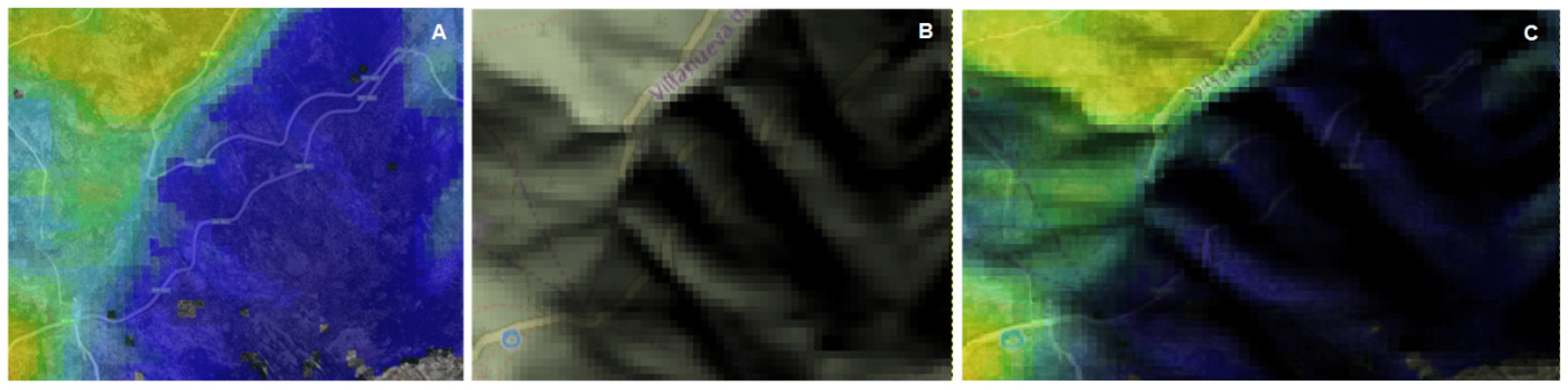
To improve the detection of these shady areas, complementary data were considered, paying special attention to the orientation of slopes. In addition, to validate the influence of these areas, a visual comparison was made using thermal images from the Landsat 8 satellite. Figure 1 presents thermal capture (A), a map with the areas identified as shaded in the same region (B), as well as an overlay of both images (C). When both images are superimposed, a clear spatial correspondence is observed, with the colder areas represented in the thermal image showing good agreement with the areas identified as shaded. This comparison supports the relevance of shading for identifying road sections that may be more susceptible to ice formation under specific local conditions. However, while this spatial relationship appears relevant at a local scale, its relevance diminishes when applied to larger-scale studies, as is the case in the present research.

2.1.5. Humidity Areas and Rainfall

The accumulation of water masses and humidity are factors that influence the severity of weather conditions and their effects on road infrastructure. After reviewing the previous literature and studies, a lack of consensus is observed on the actual influence of rivers, streams and reservoirs on extreme weather events. This uncertainty is due to the contradictory properties of water, which has both cooling capacities and buffering properties [23,24,25,26].

On the one hand, water can contribute to the cooling of an area through evaporation processes. This phenomenon can be especially significant in areas close to bodies of water, where evaporation can reduce the temperature of the surrounding air and, consequently, increase the probability of ice formation under specific conditions. However, this same capacity can vary depending on other environmental factors, such as air temperature and relative humidity. On the other hand, in situations of sudden temperature drops, water also acts as a thermal buffer. Due to its greater heat capacity, areas influenced by water tend to experience slower cooling. This means that, although the surrounding air cools quickly, water slows down the cooling process of the surface, which could limit ice formation in some circumstances [27,28].

The complexity of the interaction between water and weather conditions suggests that there is no direct element that links it to ice formation on pavements. However, the level of rainfall is found to be an influencing factor to be considered in order to characterize areas with a greater propensity for ice formation. Despite this, its influence is not considered to be of special significance in most existing studies [29,30].

2.1.6. Climatic Areas

Another important piece of information to consider in the present GIS analysis is the classification of climatic zones, established by the Technical Building Code (CTE) (Energy Savings DB H1), for Spain, as this categorization provides significant information about the severity of weather conditions [31,32].

Each climate zone is defined not only by its average temperature, but also by other relevant factors, such as humidity, solar radiation and frost duration [31]. Regarding cold mode, the classification is constituted by fives zones, where “zone 1” corresponds to the areas with milder climatic conditions, characterized by moderate winters and higher temperatures. As progression toward “zone 5” occurs, climatic conditions become increasingly extreme, characterized by severe winters with significantly low temperatures and an elevated risk of adverse meteorological events. In the context of this study, the incorporation of these climatic zones provides an additional input for identifying areas with a higher susceptibility to ice formation and other cold-weather-related hazards.

2.1.7. Winter Road Maintenance Plans

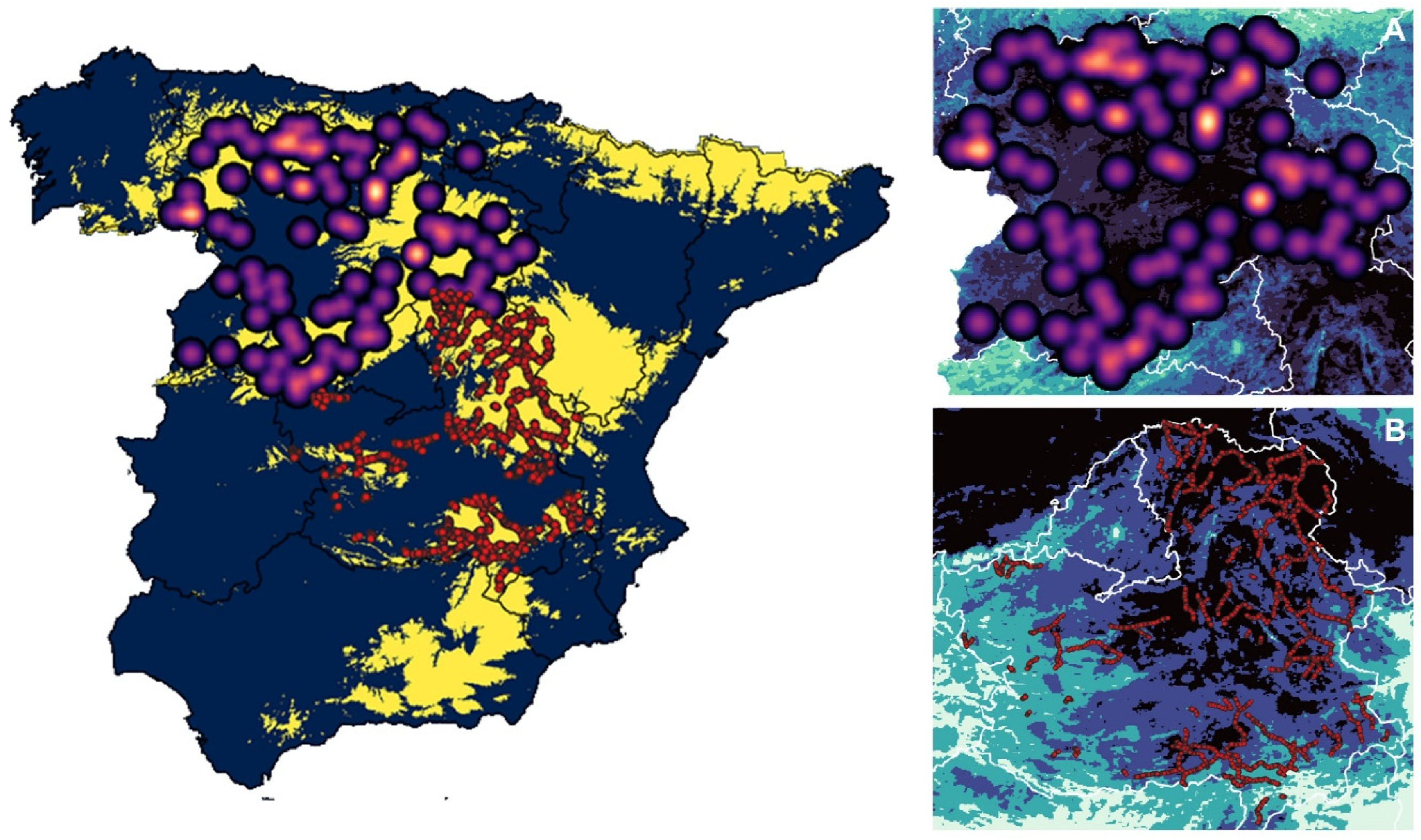
The winter maintenance plans developed by the different autonomous communities of Spain provide a useful source of information, as they not only describe winter conditions but also detail the resources available to address them, such as salt supplies, machinery, and road-clearing strategies. For this reason, a comprehensive analysis has been conducted on the resources available in each region to mitigate extreme weather conditions, with particular emphasis on cold temperatures and ice formation. As an example, Figure 2 illustrates: (A) the area of influence of existing silos overlaid with satellite temperature data for the community of Castilla y León, and (B) the integration of complex winter sections with satellite information for the community of Castilla-La Mancha. The area of influence of each silo was delineated using a weighted Voronoi approach, in which the standard Voronoi tessellation was adapted to account for differences in servicing capacity among silos. Segments served by multiple nearby silos or comprising high road-density sectors were assigned proportionally smaller influence areas, reflecting their comparatively lower per-silo servicing capacity, while isolated silos covering larger or lower-density sectors retained proportionally larger influence areas. Figure 2 also includes height (addressed in the following point) and its spatial co-occurrence with the location of the salt silos and some of the defined winter risk areas (in this case for the community of Castilla-La Mancha).

2.1.8. Height

Beyond the information derived from the road maintenance plans, another important aspect is the height (altitude) of the different sectors of the country. Therefore, this information (taken from the Digital Terrain Model—MDT25 of the IGN) has been processed and incorporated into the present geospatial evaluation. Figure 2 highlights (in yellow) all areas located above 850 m in elevation. An analysis of these zones reveals that the previously identified critical sections align closely with these high-altitude regions. This strong spatial correlation suggests that altitude is a significant factor in the occurrence of winter-related issues, reinforcing its role as a key indicator for assessing the risk of ice and snow across different areas.

However, it is important to note that while climatic zones are classified based on altitude for each province, the elevations specified in the Technical Building Code do not precisely correspond to the actual elevations observed in winter-affected areas. Although climatic zone 5 includes most of the identified sections, a significant number of areas below 850 m (in the regions evaluated) in altitude may also experience severe weather conditions. This suggests that factors beyond altitude may influence the severity of winter conditions.

2.2. Processing Methodology

2.2.1. Multivariate Analysis of Information

Multivariate analysis of geospatial data allows variables such as elevation, temperature, and precipitation to be combined with the objective of identifying complex patterns. Using raster layers, where each cell represents a geographic feature, techniques such as map algebra are applied to perform mathematical operations and obtain accurate results.

One of the initial steps in this context is the normalization of data, considered a crucial process in geospatial analysis, especially when working with multiple variables. This procedure ensures that all layers are standardized to a comparable range, which is essential for conducting meaningful analysis. In this sense, one of the most common methods for normalizing data is Min–Max scaling, which adjusts the values of each layer within a specific range, usually between 0 and 1 (Equation (1)). In the normalization process, each layer is evaluated independently, calculating its minimum and maximum values. The Min–Max scaling equation is then applied to each cell, transforming all values in the range 0 to 1. This provides a cohesive dataset that can be used for further analysis without the influence of scaling discrepancies:

$$X_{\mathit{standardized}}= {\displaystyle \frac{X- X_{min}}{X_{max}-X_{min}}}$$

(1)

where $X$ is the original value and $X_{min}$ and $X_{max}$ are the minimum and maximum values of the layer respectively [33].

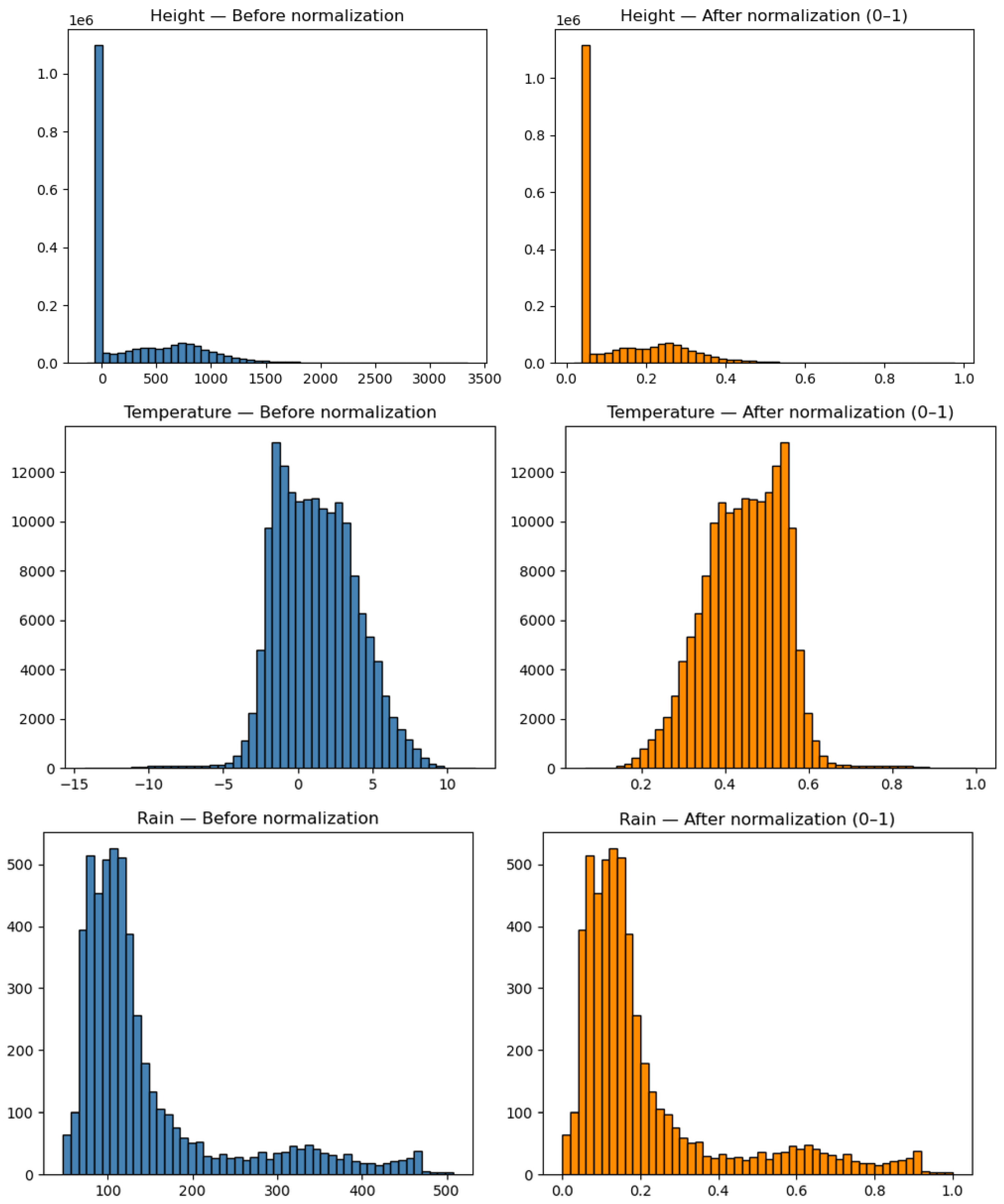
Figure 3 illustrates the effect of Min–Max normalization on the distribution of the three variables retained in the final risk index (height, temperature, and rainfall). As expected from a linear transformation, the shape of each distribution is preserved after normalization, with values rescaled to the 0–1 range. Height and rainfall exhibit a right-skewed distribution, reflecting the predominance of lowland areas and low-to-moderate precipitation values across the study area, while temperature shows an approximately symmetric distribution.

Normalization is treated as a prerequisite for index construction rather than a modeling step. Its sole purpose is to ensure numerical comparability among variables with different physical units, without implying equal physical importance.

2.2.2. Map Algebra

Map algebra has been implemented for its powerful benefits in geospatial analysis, allowing mathematical operations to be performed on raster layers by assigning weights to different variables [34]. To ensure that the weighting system is relevant and effective, a prior process of identifying key variables that should receive a higher weighting, based on their statistics and correlation, was carried out.

• Spatial assessment analysis

When multiple raster layers are available, it is essential to analyze the correlation between them to determine which ones are most strongly related to the variable of interest. This analysis allows for assigning higher weights to layers that have a closer relationship to the target variable, which can improve the accuracy of the final model.

To establish the correlation between raster variables, a data extraction process was performed, involving the creation of a point layer in ArcGIS Pro version 3.7 (Esri, Redlands, CA, USA). By applying an approach based on the Nyquist theorem and random sampling, a layer was generated that ensures an optimal amount and coverage of data. This approach ensures that the information extracted from the raster layers is representative and suitable for subsequent analysis [35].

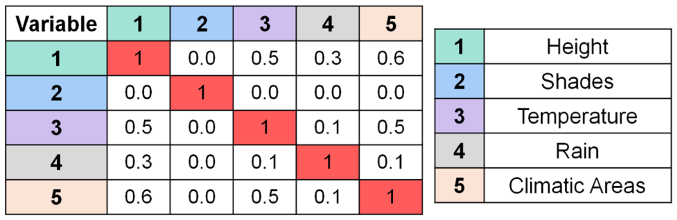
Based on the analysis of the datasets considered above, the data included in the raster layers in this research are the height (topography), shadows, precipitation, climate areas and temperature. With the data organized in a common framework, a joint correlation analysis can be conducted. This analysis involves comparing pairs of variables (layers) and examining their distribution within a two-variable system. Through this approach, the behavior of the variables concerning a linear function has been assessed, enabling the calculation of the determination coefficient (R²) for each pair. Figure 4 presents the correlation matrix data for the variables.

From the correlation matrix data, it can be observed that Variable 1 has a significant relationship with more than two variables, which highlights its influence on the general model and suggests that this variable has a considerable weight in the impact on the study areas. Conversely, Variables 3 and 5 show a strong relationship both between themselves and with Variable 1, implying that they should be assigned similar weights in the model. In contrast, Variables 4 and 2 contribute minimally to explaining the phenomenon under study, indicating their less significant influence. Based on the above, an initial model has been proposed to adjust the weighting system according to the results obtained in the correlation analysis.

Statistical significance was assessed for each pairwise relationship shown in Figure 4, using an F-test on the second-order polynomial fit (

Table 1. R² values (second-order polynomial fit) and statistical significance for each pairwise variable relationship shown in Figure 4. * low significance, ** moderate significance, *** high significance, and n.s. (not significant).

Variable Pair	R2	p-Value	Significance
Height—Shades	0.000	0.515	n.s.
Height—Temperature	0.554	<0.001	***
Height—Rain	0.314	<0.001	***
Height—Climatic Areas	0.643	<0.001	***
Shades—Temperature	0.007	<0.001	***
Shades—Rain	0.004	<0.001	***
Shades—Climatic Areas	0.018	<0.001	***
Temperature—Rain	0.131	<0.001	***
Temperature—Climatic Areas	0.565	<0.001	***
Rain—Climatic Areas	0.109	<0.001	***

). All relationships were statistically significant (p < 0.001) except for the Height–Shades pair (p = 0.515, n.s.), consistent with its negligible R² value. It should be noted that, given the large sample size used in this analysis, statistical significance is reached even for weak relationships (e.g., R² < 0.05); therefore, the R² values reported in Figure 4 remain the primary indicator of the practical strength of each relationship, with statistical significance provided as complementary confirmation.

• Principal Component Analysis (PCA)

In this study, Principal Component Analysis (PCA) is used exclusively as an exploratory tool to assess redundancy, collinearity, and relative influence among variables. PCA results do not directly define the structure of the winter risk equation but inform variable selection and weighting decisions.

This distinction is essential: the final risk index is not a PCA-derived score, but a weighted combination of selected variables guided by exploratory analysis and operational reasoning.

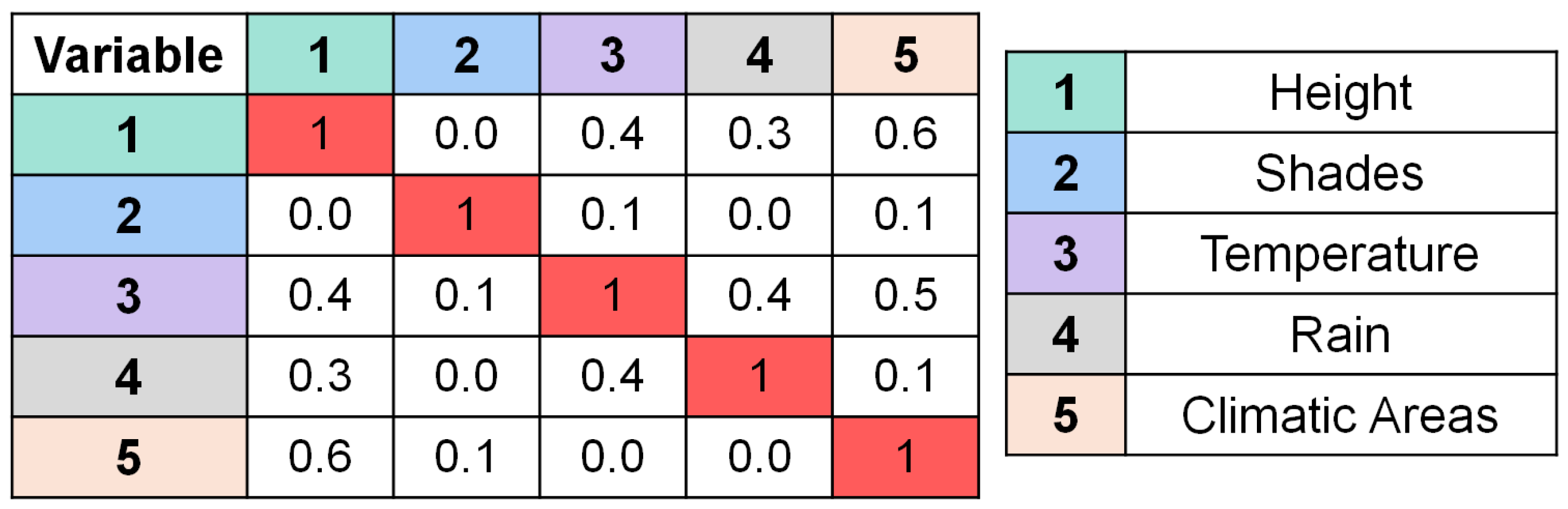
This method allows the identification of the variables (raster layers) that better explain the variability in the data set. PCA contributes to identify the most influential layers within the study, allowing for the appropriate assignment of weights in the final model. PCA reveals significant correlations between several bands obtained, showing that the increase or decrease of a variable (band) affects or is influenced by another variable [36,37,38]. To define the assignment of weights, an exhaustive analysis of the bands obtained in the PCA was carried out. By comparing the different bands and calculating their correlation, a matrix was generated that allows the identification, through the R² values, of the degree of significance of each variable with respect to a second-order polynomial model.

The correlation matrix (Figure 5) reveals that Variable 1 is the most significant, with a strong connection to Variables 3, 4 and 5. Variable 3 also contributes relevant information on Variable 1 and 4, while Variable 5 is strongly dependent on Variable 1. In contrast, Band 2 has a minimal contribution, suggesting its possible exclusion or assignment of a very low weight. Therefore, on a large scale, this factor does not have significant relevance in identifying the risk addressed in this work.

Table 2. Eigenvalues and percentage of variance explained by each principal component.

Principal Component	Eigenvalue	% Variance	% Cumulative Variance
PC1	1.629	51.17	51.17
PC2	0.532	16.70	67.87
PC3	0.488	15.33	83.20
PC4	0.421	13.22	96.41
PC5	0.114	3.59	100.00

reports the eigenvalues and the percentage of variance explained by each principal component, calculated from the standardized (z-score) input variables to avoid scale-dependent bias. The first component accounts for 51.17% of the total variance, followed by 16.70% for the second and 15.33% for the third, together explaining 83.20% of the cumulative variability in the dataset. No single component dominates disproportionately, indicating that the variability in the dataset is distributed across multiple environmental factors rather than driven by a single variable with a large numerical scale.

2.2.3. Variable Selection and Normalization

After compiling and analyzing the influence of each of the inputs considered for the assessment of winter risk in road infrastructure, the following conclusions have been drawn:

-

The observed spatial relationship between winter maintenance plans and Climate Zone 5 indicates that the areas identified for winter maintenance are generally associated with the most climatically severe regions. However, climatic zoning alone is insufficient to explain the spatial occurrence of winter hazards, as ice formation is also influenced by local factors such as topography, altitude, precipitation, and surface temperature. This finding highlights the need to integrate multiple geospatial variables to achieve a more accurate identification of vulnerable road sections.

-

Climate zone 4 exhibits transitional characteristics with climate zone 5, frequently experiencing comparable climatic conditions. Therefore, its inclusion in the analysis is critical, as it encompasses numerous sections susceptible to similar winter-related issues.

-

Climate zones 3, 2, and 1 are excluded from the present analysis due to their low likelihood of experiencing snow and ice-related issues. This indicates that winter-related risks are generally more prevalent in regions with higher altitude and greater climatic severity.

-

The strong correlation between altitude and temperature confirms the expected climatic relationship between both variables. Nevertheless, they were retained in the model because they provide complementary information, with altitude representing long-term spatial susceptibility and temperature capturing the dynamic meteorological conditions associated with winter hazards.

-

Despite the existing correlation with the climatic zones defined by the CTE, a more flexible categorization is required to allow for better differentiation between the different affected areas.

-

Based on all correlation analyses, the variables to be considered in the geospatial analysis for winter mode are, in order of priority, satellite temperature, altitude, climatic zones 5 and 4, and rains. It should be mentioned that shadows have been discarded due to the low correlation that exists when the analysis is carried out on a large scale. Therefore, despite the significant correlation observed in Section 2.1.4, the inclusion of this factor is not deemed appropriate given the scale of the present study. It is worth noting that climatic zones do not correlate strongly with the shadow layer, which is expected given the difference in spatial scale and nature between both variables: climatic zones represent a coarse, regionally aggregated classification (five categories at national scale, following CTE criteria), whereas the shadow layer reflects fine-scale, local topographic shading effects. This scale mismatch, rather than indicating an inconsistency in the climatic zone variable, supports its retention as an independent, non-redundant input, distinct from the locally-derived shadow information.

-

Based on the previous matrix analyses, the variables most influential in identifying the risk pursued in this research are deduced. Given the difficulty of establishing a direct relationship between these results and assigning their relevance in risk estimation, it is considered appropriate to give equal weight to temperature and altitude variables, and to a lesser extent to precipitation. Likewise, climatic zones are only considered when delimiting the sectors corresponding to zones 4 and 5.

To evaluate the robustness of this correlation- and experience-based weighting scheme, an entropy weighting method was additionally applied to the same normalized variables (height, temperature, and rainfall). This approach, based on Shannon’s entropy, assigns weights according to the information content and variability of each variable, independently of expert judgement. The resulting entropy-derived weights were 0.523 for height, 0.343 for temperature, and 0.134 for rainfall. This confirms the same overall hierarchy adopted in the heuristic model, with rainfall retaining the lowest weight among the three variables. However, the entropy method attributes a somewhat larger relative weight to rainfall than the heuristic scheme (0.134 vs. 0.048, normalized), and a less equal distribution between height and temperature than initially assumed. These results support the general validity of the correlation-based weighting adopted in Equation (2), while suggesting that the relative contribution of rainfall may warrant further refinement in future iterations of the model.

The entropy-derived weights were not directly incorporated into the final risk index because the entropy method evaluates the relative information content and spatial variability of each variable, rather than its physical or operational relevance to winter road hazards. In the present study, entropy weighting was therefore used as an independent robustness assessment of the weighting hierarchy adopted from the combined correlation analysis, PCA results, physical interpretation, and operational considerations. The consistency between both approaches, particularly the dominant contribution of altitude and temperature and the lower relative importance of rainfall, provides additional support for the adopted weighting structure. Nevertheless, future developments of the model could evaluate entropy-derived weights as an alternative configuration and compare their performance against independent observations of winter-related road events.

In this way, the result of quantifying the risk associated to winter conditions can be summarized as Equation (2) shows:

$$R_W=N_H+N_T+(0.1·N_R)$$

(2)

where $R_W$ is the winter risk and $N_H$, $N_T$, and $N_R$ are the normalized values of the variables height, temperature and rains, respectively.

It must be also mentioned that rainfall data were originally provided in geographic coordinates (WGS84), with a native cell size of 0.1° (129 columns × 79 rows, 10,191 cells), consistent with the resolution of the source climatic dataset. Snow-risk zones were derived from national cartographic sources in a projected coordinate system, with a native cell size of 3440.13 m (300 columns × 251 rows, 75,300 cells). Both grids, together with the remaining raster layers described in Section 2.1, were resampled and reprojected to a common analysis grid, in a shared projected coordinate system, prior to the correlation and map algebra analysis described in Section 2.2, ensuring spatial consistency across all variables despite differences in native source resolution.

2.3. Quantitative Validation Methodology

The spatial consistency of the winter risk model was quantitatively evaluated using independent spatial datasets not involved in the model construction. Validation was performed by assessing the spatial association between the continuous winter risk index, the ice-related observation centroids and the winter maintenance infrastructure (salt silos).

The adopted validation strategy is grounded in the concept of spatial enrichment and exposure consistency, commonly used when the target variable represents persistent susceptibility rather than discrete event prediction. In the absence of exhaustive road-level observations of winter hazard occurrences, this validation focuses on assessing whether independent indicators of winter-related exposure and operational response are preferentially concentrated within the highest risk classes defined by the model. This approach enables an objective evaluation of the model’s ability to capture long-term spatial patterns of winter risk using independent datasets of different nature.

As defined in the previous section, the winter risk model produces a continuous scalar field $R\left(x\right)$ over the spatial domain $\mathsf{\Omega }\subset {\mathbb{R}}^2$, where higher values indicate increased susceptibility to winter-related hazards. To enable an objective comparison between the spatial distribution of independent point-based observations and the risk surface, the continuous index was partitioned into equal-area quantile classes. This approach ensures that each class represents the same proportion of the study area and therefore provides a known baseline probability under spatial randomness.

Formally, the spatial domain was divided into $K$ quantiles as the following Equation (3) presents:

$${\mathsf{\Omega }}_k=\left\{x\in \mathsf{\Omega }|Q_{k-1}<R\left(x\right)\le Q_k\right\}, \left|{\mathsf{\Omega }}_k\right|={\displaystyle \frac{1}{K}}\left|\mathsf{\Omega }\right|$$

(3)

where $Q_k$ denotes the $k$-th quantile of the cumulative distribution of $R\left(x\right)$. In this study, $K=5$ (quintiles), so that each class represents 20% of the total area.

To quantify the degree of spatial association between observed ice-related events and high-risk areas, an enrichment metric (Lift) was computed. Lift is defined as the ratio between the observed proportion of events located within a given risk class and the proportion of area occupied by that class (Equation (4)):

$$Lift\left(Q_i\right)={\displaystyle \frac{P\left(event|Q_i\right)}{P\left(Q_i\right)}}$$

(4)

where $P\left(Q_i\right)$ is the fraction of the $i$-th quantile area. Lift values close to unity indicate spatial independence, whereas values greater than one indicate a positive spatial association between observed events and areas classified as high risk by the model.

Two independent datasets were therefore considered for validation. First, ice-related observation (points extracted from road sections included in the official winter maintenance plans) were treated as realizations of winter hazard occurrences, and their distribution across risk quantiles was evaluated using the enrichment-based metric described above. Second, winter maintenance silos were used as an independent operational dataset reflecting long-term infrastructure planning. Although silos are not expected to coincide exactly with hazardous road sections, their spatial distribution relative to high-risk areas provides complementary validation of the model. In this case, enrichment within the upper risk quantiles (Q5 and Q4–Q5) was evaluated to assess whether infrastructure is preferentially located in areas identified as most susceptible to winter hazards.

This validation framework enables an objective assessment of the model’s predictive consistency using independent datasets of different nature, combining physical observations and operational decision-making while relying on reproducible, enrichment-based spatial metrics.

3. Results

3.1. Global Winter Risk Map

As explained before, the spatial analysis for the creation of the winter risk map has considered several crucial layers of information for the identification and assessment of the area’s most vulnerable to severe cold conditions. Based on this initial data, a series of preliminary correlation maps have been generated.

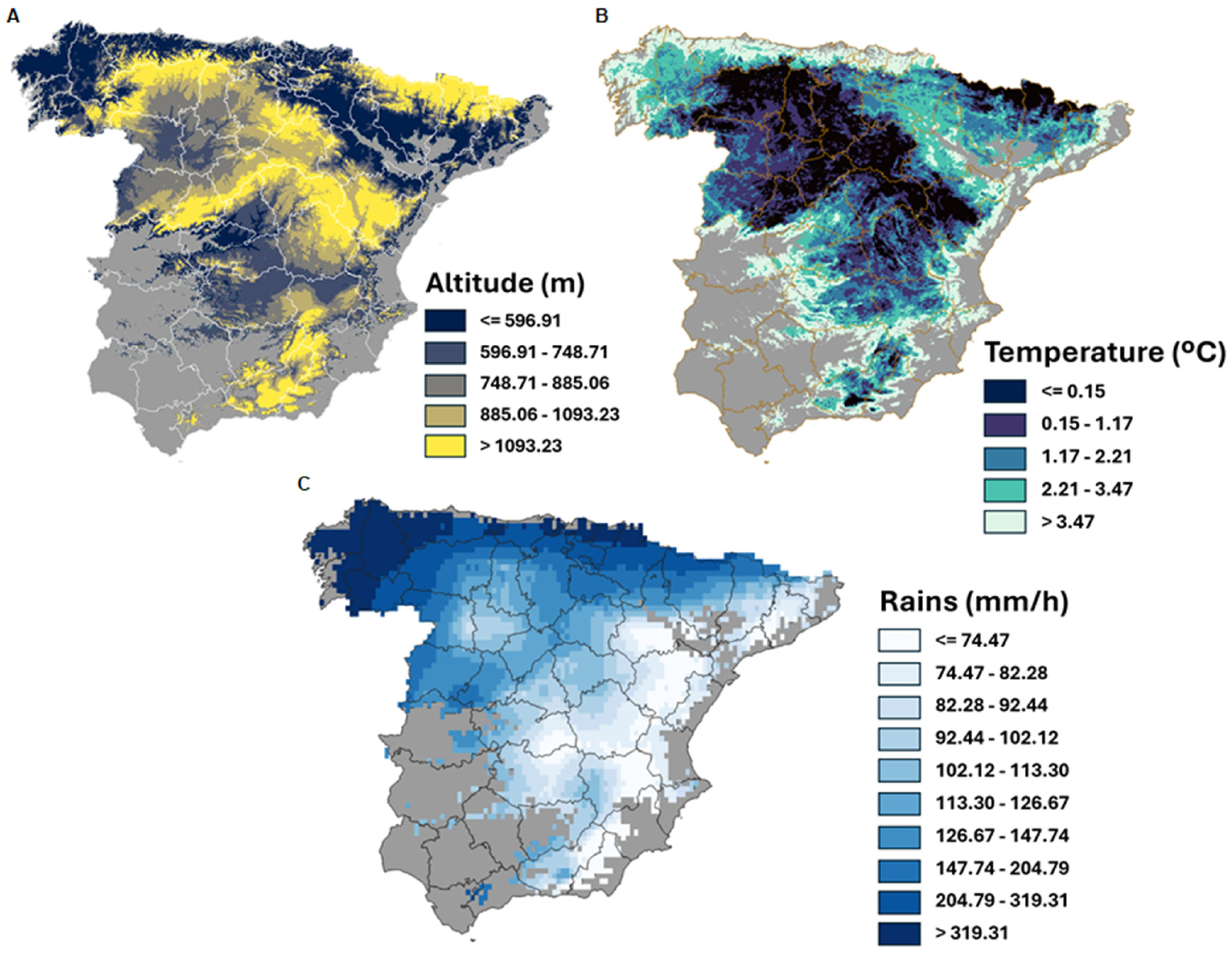
• An altitude map (Figure 6A) that provides a comprehensive view of how these factors influence winter risk. Higher altitude areas are usually more prone to extreme conditions, such as snow accumulation and frost.
• A temperature map, derived from the satellite thermal data, was generated (Figure 6B), selecting only the relevant data corresponding to areas exceeding the identified risk threshold. This filtering process excluded non-critical temperatures, allowing a focus on the lowest values, which indicate higher winter risk. This refinement enabled a more targeted analysis of areas requiring priority attention.
• A rain map (Figure 6C), also obtained from the satellite information, where precipitation data has been filtered to focus only on the area of interest, discarding values that do not contribute to the winter risk assessment. This approach has facilitated a clearer understanding of how snowfall impacts the areas of greatest risk, allowing for more accurate and efficient resource planning.

Figure 6. (A) Altitude map; (B) temperature distribution; and (C) Rains map of the case under study, average rainfall for the month of January over the last 10 years (GPM IMERG V6). Data for each variable are shown for the selected climatic zones.

Figure 6. (A) Altitude map; (B) temperature distribution; and (C) Rains map of the case under study, average rainfall for the month of January over the last 10 years (GPM IMERG V6). Data for each variable are shown for the selected climatic zones.

Finally, using the winter risk index defined in Section 2.2, a global winter risk map was generated for the national road network. The variables considered were normalized: altitude values were scaled from 0 (lowest) to 1 (highest), temperature values were inversely normalized so that lower temperatures (higher risk) approach 1, and rainfall was normalized with a reduced weight of 0.1 due to its minor influence on the assessed risk. The resulting index ranges from 0 to 1, with higher values indicating greater exposure to winter-related hazards [35].

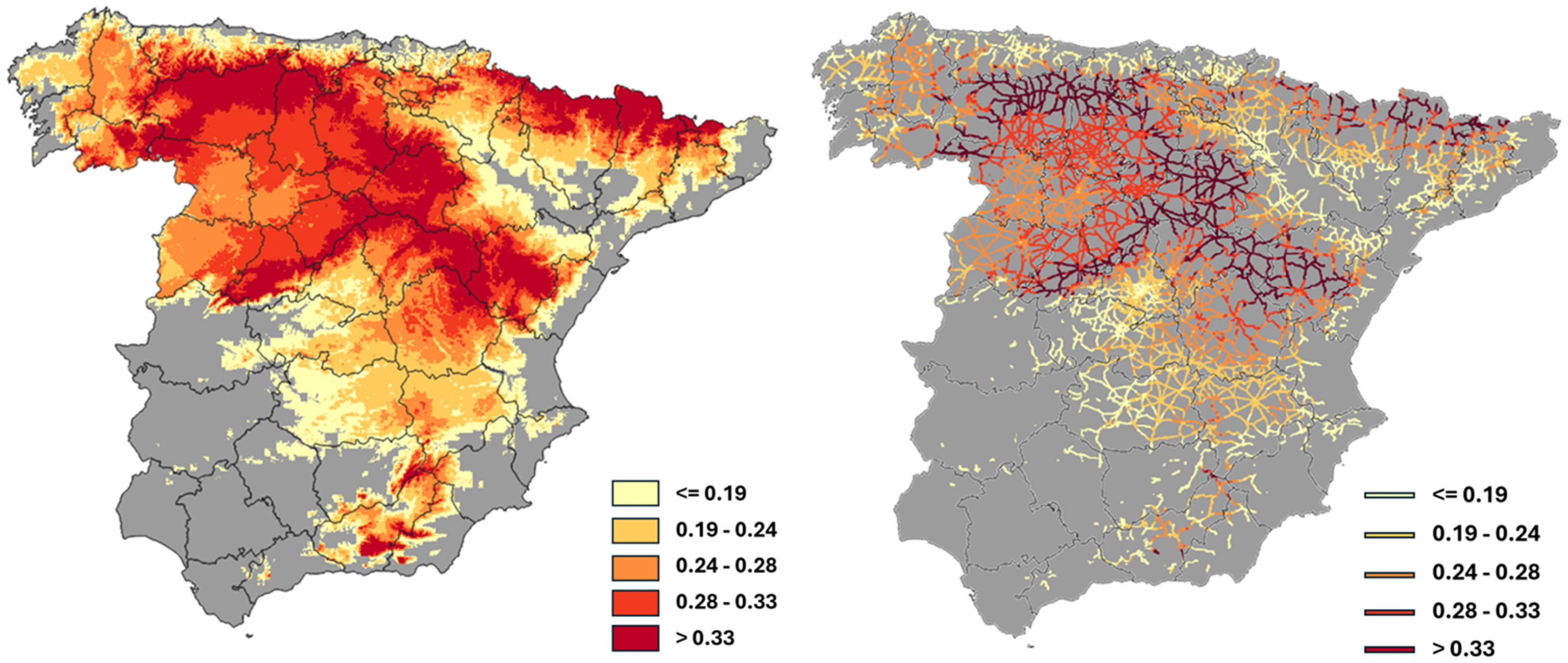
The final winter risk map and its implementation on the global road infrastructure of the country are presented in Figure 7. As mentioned, results are shown normalized to a range from 0 to 1, where 1 represents the highest risk level and 0 the lowest one.

Figure 7. Final winter risk map (left) and its application to the road infrastructure of the case under study (right).

Figure 7. Final winter risk map (left) and its application to the road infrastructure of the case under study (right).

3.2. In-Depth Analysis of a Specific Sector

Based on the final map included in the previous section, a more detailed analysis has been conducted on one of the areas at highest risk of exposure to cold weather conditions. Therefore, the region of Ávila (at the center of the country) has been chosen, as it includes different risk levels, with a significant portion of its area falling under the highest risk category. This province, located within the Castilla y León community, experiences a Mediterranean continental climate, heavily influenced by its altitude, leading to cold winters and hot summers. The area faces several meteorological issues in winter due to its altitude and location, with extreme temperatures that can drop below −10 °C in some parts, especially in the mountains. However, there are notable variations between its different areas, which affect the distribution of winter risk.

Although the detailed spatial analysis focuses on the province of Ávila, the quantitative validation of the winter risk index incorporates independent observational and operational datasets that extend beyond its administrative boundaries into adjacent regions of Castilla y León and Castilla-La Mancha. This broader spatial extent reflects the regional organization of winter maintenance infrastructure and the spatial distribution of ice-related observations, which are not confined to provincial limits. Incorporating these datasets allows for a more robust and representative evaluation of the model’s predictive consistency under comparable climatic and geomorphological conditions.

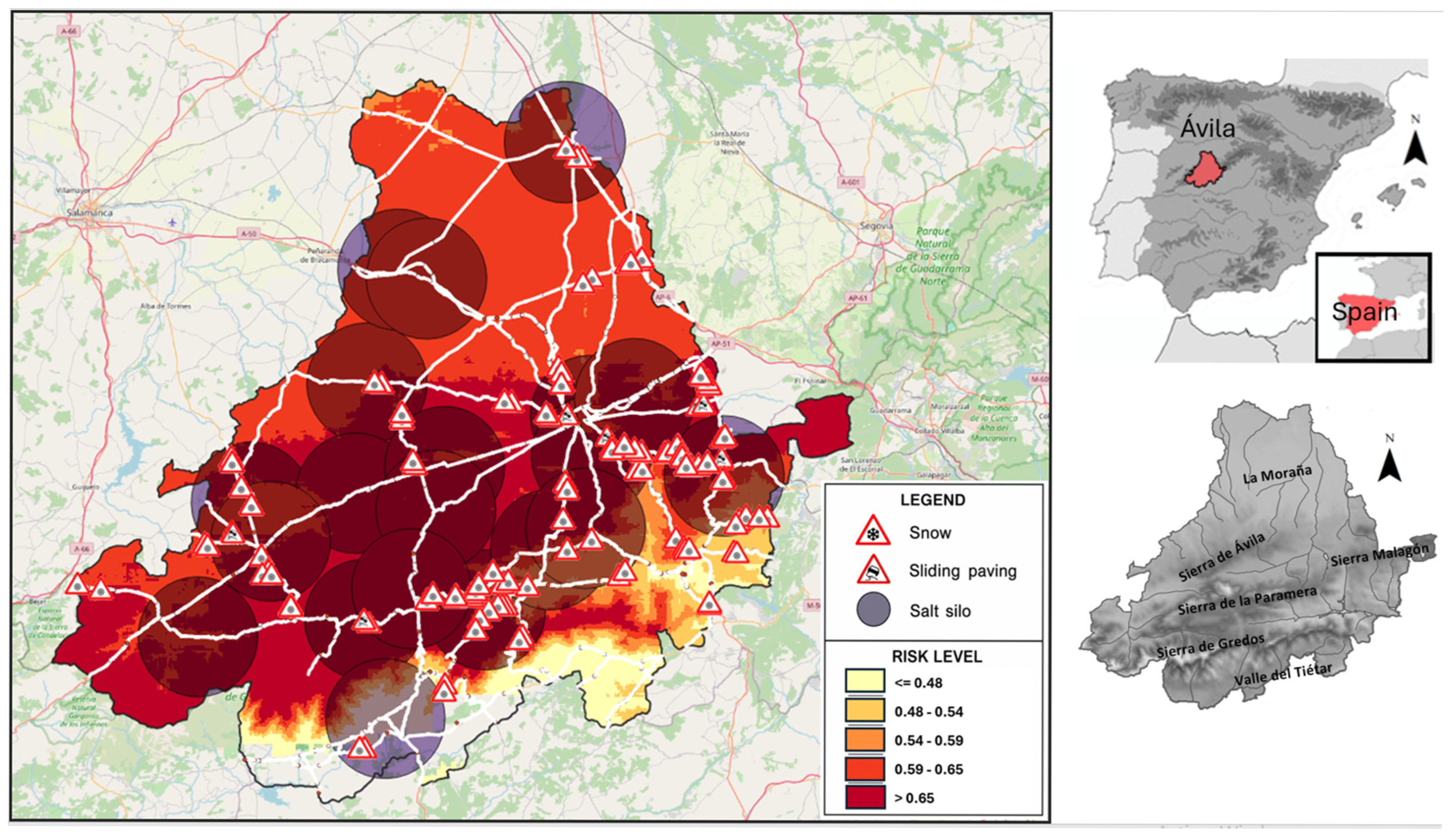
As can be observed in Figure 8, the highest-risk zones lie in the Sierra de Gredos, Sierra de Ávila, and the province’s central area. The Sierra de Gredos in the south endures long, sub-zero winters and heavy snowfall at high altitudes, increasing avalanche risk. Likewise, the Sierra de Ávila and Paramera range in the center-northwest suffer constant frost and frequent snow due to their medium-high elevations and climatic barrier effect. In the central Amblés Valley and Ávila city, both above 1000 m, intense frosts and recurrent snowfalls are common. Conversely, La Moraña to the north experiences lower altitudes and less winter precipitation (though frost persists), while the Tiétar Valley benefits from milder conditions thanks to mountain shelter, reducing low-altitude snowfalls. Overall, altitude, continentality, precipitation patterns, and cold winds drive Ávila’s winter risk, concentrating it in high, exposed terrain and sparing the northern plains and Tiétar Valley.

In order to validate the winter risk geospatial model in the aforementioned province of Ávila, two key elements in road management and prevention were analyzed; ice warning signs and the distribution of salt silos.

Ice warning signs mark road segments prone to winter hazards such as ice sheets or snow accumulation. Installed by road authorities in locations with persistent winter hazards, such as high-altitude or low-sunlight areas, these signs provide an additional empirical benchmark for model validation. Their locations (Figure 8) were manually identified using online cartographic services and incorporated into the GIS database. Comparing their spatial distribution with the winter risk map confirms a strong correspondence between the model-identified high-risk zones and the actual warning sign locations.

Additionally, an analysis of the salt silo’s locations (provided by the Junta de Castilla y León) was conducted. These silos are critical for winter road management, as they store and distribute materials for preventive and corrective road treatment during extreme cold events. The study examined the location and capacity of these silos in relation to areas with the highest snowfall and frost occurrences. As can also be deduced from Figure 8, the greatest number and density of silos are found in the area categorized as greatest risk (>0.65).

To complement the visual inspection shown in Figure 8, quantitative validation metrics were computed for both ice-related observation centroids and winter maintenance silos. Thus,

Table 3. Summary of the ice-related observation centroids.

Id	Metric	Value
0	Valid centroids (N)	13,081.00
1	Excluded centroids (NoData)	0.00
2	Centroids in Q5 (%)	54.36
3	Centroids in Q4–Q5 (%)	100.00
4	Lift (Q5)	2.72
5	Lift (Q4–Q5)	2.50

summarizes the quantitative validation results obtained using ice-related observation centroids. A total of 13,081 valid centroids were evaluated, with 54.36% falling within the highest winter risk class (Q5), yielding a lift value of 2.72. All centroids were located within the combined upper risk classes (Q4–Q5), indicating a strong spatial association between observed ice-related hazards and areas classified as high risk by the model.

In addition,

Table 4. Validation reports of winter maintenance silos.

Id	Validation Type	Metric	Value
0	Winter maintenance silos	Silos (N)	116.00
1	Winter maintenance silos	Silos in Q5 (%)	48.28
2	Winter maintenance silos	Silos in Q4–Q5 (%)	85.34
3	Winter maintenance silos	Lift (Q5)	2.41
4	Winter maintenance silos	Lift (Q4–Q5)	2.13

reports the corresponding validation metrics for winter maintenance silos. Approximately 48.28% of the silos are located within Q5, resulting in a lift value of 2.41, while 85.34% fall within the combined upper risk classes (Q4–Q5). Although silo placement reflects long-term operational planning rather than direct hazard observations, these results indicate a consistent alignment between the modeled winter risk patterns and preventive infrastructure distribution.

Together, these results provide quantitative evidence of a spatial association between the modeled winter susceptibility patterns, the available ice-related observations, and the distribution of winter maintenance infrastructure at a regional scale.

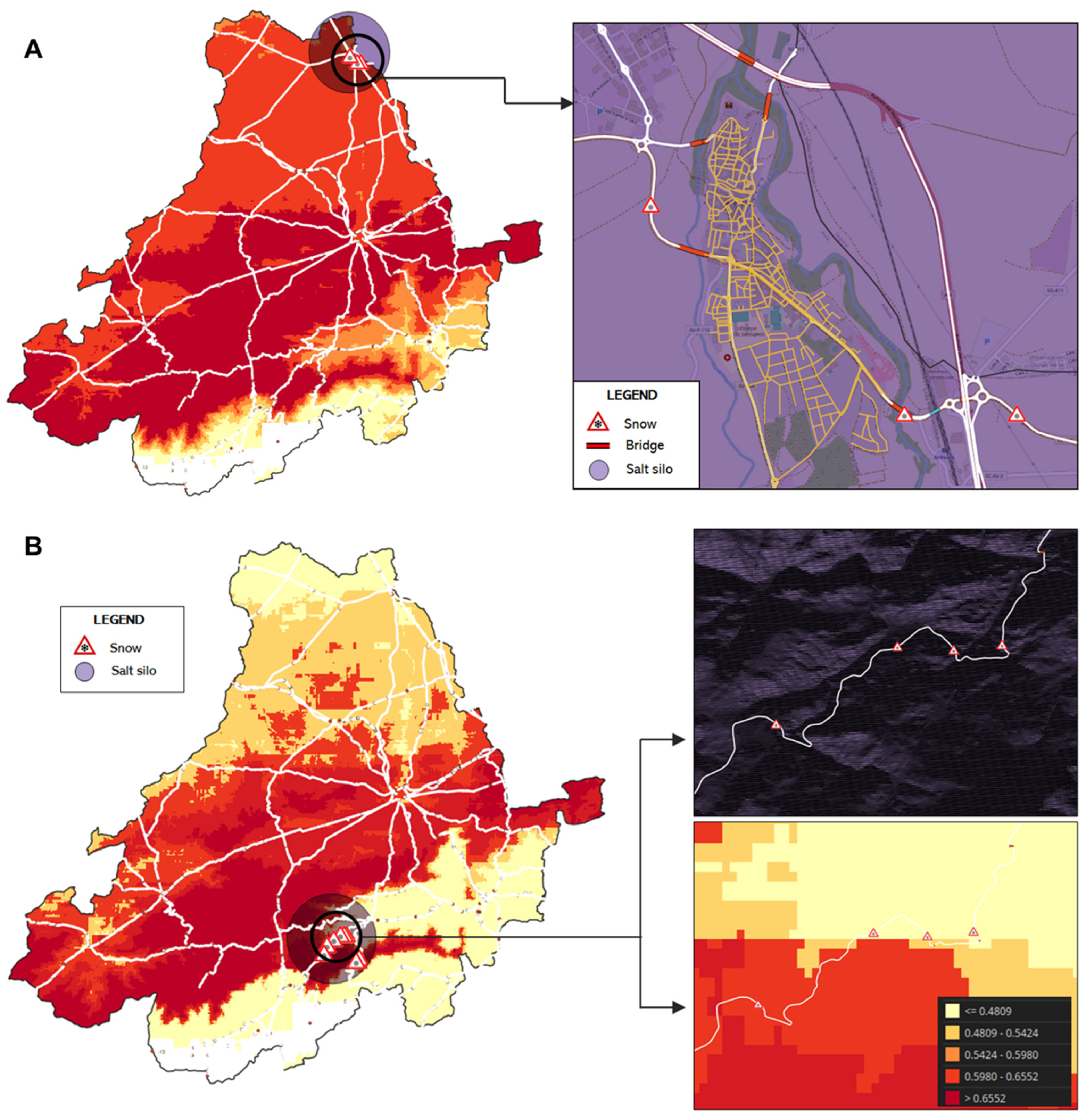
In general terms, strong spatial correspondence is observed between the concentration of warning signs for ice or snow conditions and salt silos and the areas identified as most at risk by the developed geospatial model. In any case, all indicators of the region’s winter plans fall within the areas marked as at risk in the viewer shown in Figure 8. However, it is interesting to conduct a more detailed analysis in areas that, despite being consistent with the model results, are not located in the highest risk zone (dark red). This occurs in the northernmost part of the province, categorized with a risk of 0.59–0.65 (not the most extreme risk), but where the location of a salt silo and several warning signs of possible ice or snow formation are detected (Figure 9A).

Upon closer examination of the designated area, the presence of elevated structures, such as bridges and overpasses, was identified using automatically classified road infrastructure data obtained from online cartographic services. These elements, exposed to extreme weather conditions, lose heat more quickly than ground contact surfaces, increasing their vulnerability to ice formation. Consequently, they pose additional hazards under extremely low-temperature conditions compared to the conventional road network.

To further evaluate the performance of the proposed methodology, an additional area within the study region was selected for detailed analysis. This area was chosen because it presents a high concentration of warnings and interventions included in the provincial winter maintenance plan, providing an opportunity to compare the model predictions with existing operational practices. A more detailed analysis of the specified area using the GIS-based model indicates that it is not situated in a region with relevant terrain features or crossing infrastructure as in the previous scenario. Given this, and to further refine the assessment, the shadow map generated from the Digital Terrain Model (MDT25) was integrated into the analysis. Upon examining Figure 9B, spatial correspondence is observed between the locations of snow warning signs and the shadowed areas, which are represented by darker black regions on the shadow map. This spatial correspondence suggests that terrain-induced shading may contribute to local snow persistence and associated winter hazard conditions.

4. Discussion and Conclusions

4.1. Spatial Performance and Interpretation of the Geospatial Model

The geospatial evaluation included in this research is designed to systematically identify and assess the road infrastructure segments most vulnerable to extreme weather conditions, focusing on prolonged exposure to low temperatures (winter mode). These adverse climatic conditions can significantly impact road safety and operational efficiency, increasing the likelihood of hazardous driving conditions, disruptions in traffic flow, and potential infrastructure degradation. Ensuring the resilience of road networks in the face of such environmental challenges is critical for maintaining safe and reliable transportation systems, particularly in regions prone to harsh winter conditions.

To achieve this objective, the developed model integrates the key climatic and environmental variables influencing winter road risk. By incorporating these key factors, the model is able to generate a detailed and data-driven winter risk assessment of the entire territory of Spain. The final output is presented in the form of a winter risk map, which visually represents the varying levels of exposure and vulnerability across the assessed road network. Given that in many cases the practices included in winter viability plans are carried out in a generalized and conservative manner, this map serves as an essential decision-making tool for road authorities and infrastructure managers, enabling them to prioritize maintenance efforts, implement targeted mitigation strategies, and enhance overall road safety during winter months.

The quantitative validation based on independent observational and operational datasets supports the internal consistency of the proposed winter risk index. Although the model is not intended to predict individual hazard events, but rather to characterize persistent spatial exposure patterns, the systematic concentration of ice-related observations and winter maintenance infrastructure within the highest-risk classes suggests that the index effectively captures long-term spatial exposure to winter hazards. The agreement between model outputs and operational planning decisions further indicates that the risk patterns identified by the model are meaningful at a regional scale.

In addition to providing a broad-scale assessment of winter risk, the model leverages its interactive capabilities to allow users to conduct detailed analyses of specific areas of interest. This functionality enables users to closely examine critical sections of the road network and identify additional factors that may contribute to an elevated risk level. By zooming into a particular area, users can assess micro-scale conditions that may not be fully captured in the broader risk classification. Key aspects that can be evaluated include the extent and persistence of shadowed areas, as well as the presence of unusual or site-specific elements within the road infrastructure that could exacerbate winter hazards. This level of granularity ensures that the risk assessment process remains dynamic and adaptable, accommodating site-specific considerations that may not be immediately apparent in the overall winter risk map. Ultimately, this feature strengthens the geospatial model utility as a decision-support system, helping to improve winter road safety by facilitating proactive maintenance strategies, targeted intervention measures, and optimized resource allocation.

The results also provide insight into the different spatial roles of the variables considered in the winter risk assessment. Altitude emerges as one of the dominant factors because it represents a persistent influence on regional winter susceptibility, being generally associated with lower air and surface temperatures and with environmental conditions that may favor frost and snow persistence. Although altitude and temperature are correlated, their roles are complementary rather than redundant: altitude represents a relatively stable territorial control, whereas satellite-derived temperature captures the spatial expression of thermal conditions during the analyzed period. The relevance of geographical parameters, including altitude, in explaining spatial variations in road surface temperature has also been highlighted in previous GIS-based road weather studies [39]. In contrast, the lower relevance of the shadow layer at the national scale appears to be mainly related to its strongly localized nature. Terrain-induced shading depends on local topography, road orientation, surrounding obstacles, and solar geometry, and its influence may therefore become diluted when assessed across a heterogeneous national territory. Previous route-based studies have demonstrated that shading and sky-view conditions can significantly influence local road surface temperature distributions [40], supporting the relevance of these factors at detailed spatial scales. Similarly, GIS-based assessments of winter snow susceptibility have identified elevation and slope aspect as relevant environmental controls, partly through their influence on solar exposure and local thermal conditions [41]. Therefore, the limited contribution of shading to the national-scale index should not be interpreted as an absence of physical influence, but rather as evidence of its scale-dependent character.

4.2. Model Validation and Future Developments

The overall results of the geospatial model show a consistent spatial correspondence between the areas classified as high risk and the winter viability plans implemented in the different regions. This agreement supports the ability of the proposed framework to identify spatial patterns associated with increased susceptibility to adverse winter conditions. A representative example is observed in the province of Ávila, where areas identified by the model as having higher winter risk show good spatial agreement with existing winter mitigation actions and operational infrastructure. These results provide additional evidence of the spatial consistency of the proposed risk index and its potential to complement existing regional knowledge and support decision-making processes.

Although the quantitative validation performed in this study shows a consistent spatial association between the highest-risk classes and independent indicators related to winter exposure and maintenance infrastructure, the scope of these results should be clearly acknowledged. The validation framework primarily evaluates the spatial consistency of the susceptibility patterns represented by the index and does not constitute a complete assessment of its temporal predictive performance against observed winter events. A more comprehensive predictive validation would require independent and temporally referenced datasets, such as georeferenced historical records of road icing events, winter-related accidents, or specific winter maintenance interventions. The lack of such information with homogeneous spatial and temporal coverage at the national scale represents a limitation of the present study. Future incorporation of these datasets would allow the ability of the index to anticipate specific events to be evaluated and would complement the spatial validation developed in this work.

From an operational perspective, the GIS-based framework offers practical advantages for refining winter road maintenance strategies. Current winter management practices often rely on broad preventive measures, such as the widespread application of chemical anti-icing agents across extensive road sections. Although effective, these approaches can be resource-intensive and may exceed actual needs in certain locations. By providing a higher-resolution spatial assessment of winter risk, the model enables the identification of specific road segments where interventions are most critical. This supports a more targeted allocation of resources, reducing unnecessary chemical usage while ensuring adequate protection in the most vulnerable areas. Moreover, the spatially explicit nature of the model allows winter mitigation strategies to be adjusted dynamically in response to evolving weather conditions and localized terrain influences. To facilitate the practical implementation of the proposed framework, the winter risk classification can be directly linked to differentiated maintenance strategies. Road sections classified as high risk should be prioritized for continuous monitoring, preventive anti-icing treatments before forecast freezing events, and rapid deployment of maintenance crews during adverse weather conditions. Medium-risk sections may be managed through scheduled inspections and preventive treatments when meteorological forecasts indicate a high probability of ice formation, while low-risk sections can be addressed through routine surveillance and corrective interventions only when required. Although the proposed methodology supports this prioritization process, the specific de-icing procedures, treatment frequencies, and chemical application rates should be defined by the corresponding road authorities according to local regulations, pavement characteristics, traffic intensity, meteorological forecasts, and the type of de-icing agents employed.

Beyond the current capabilities of the geospatial framework, further advancements are considered to enhance its applicability and overall versatility. Several key aspects have been identified as priority areas for improvement, ensuring that the developed model continues to evolve and provide increasingly valuable insights for road infrastructure management under extreme weather conditions.

• One significant area for future development is the expansion of shadow mapping and the identification of unique elements within road infrastructure. While the model already incorporates certain terrain-based factors, refining the assessment of shadowed areas and their duration (along with incorporating additional structural elements such as bridges, tunnels, and embankments) can further improve the precision of the risk estimation. To achieve this, a more detailed weighting system should be developed, allowing these factors to be integrated into the overall risk model based on their specific influence on winter hazard formation. In this sense, a further improvement would consist of explicitly incorporating bridges, viaducts and other elevated structures into the winter risk model through a dedicated correction factor, enabling a quantitative assessment of their influence on ice formation and allowing comparison between models with and without structural corrections.
• Additionally, to increase the geospatial system versatility and extend its utility beyond winter risk assessment, the incorporation of summer-mode risk estimation is proposed. This enhancement would focus on evaluating exposure to high temperatures and its effects on road infrastructure, particularly in regions where extreme heat poses significant challenges. High temperatures can contribute to asphalt degradation, pavement softening, and an increased likelihood of thermal expansion-induced structural failures. By developing a complementary risk assessment model for heat-related hazards, the model could assist in prioritizing maintenance efforts and implementing proactive strategies to ensure road network resilience under both extreme cold and extreme heat conditions.

In general terms, the approach presented in this research provides additional spatial information for identifying road sections that may be particularly susceptible to adverse winter conditions. By supporting the identification of higher-risk areas, the geospatial model can contribute to the planning of preventive measures and pavement maintenance. Its spatially explicit framework provides a data-driven basis for refining current strategies and supporting the prioritization of interventions where they may be most needed. In this context, the proposed approach may contribute to more targeted resource allocation and decision-making related to road safety and infrastructure maintenance. Overall, the methodology provides a framework for complementing existing winter maintenance practices with spatially differentiated information on winter susceptibility.

The model’s ability to assess winter risk with greater accuracy not only helps prioritize the allocation of resources but also contributes to more effective decision-making in terms of road safety and infrastructure preservation. Ultimately, the presented analysis allows for the optimization of existing practices and the implementation of more effective, site-specific measures based on predictive data. As a result, this development significantly contributes to enhancing the safety, sustainability, and operational efficiency of road networks exposed to winter conditions.

A final issue that should be discussed is the ecological perspective. As commented, in addition to improving operational efficiency, the proposed risk-based maintenance strategy has the potential to reduce the environmental impacts associated with winter road maintenance. By enabling interventions to be concentrated on the road sections with the highest probability of icing, the methodology may reduce unnecessary applications of de-icing agents on low-risk segments. This targeted approach could contribute to minimizing soil and water contamination, vegetation damage, and the corrosion of road infrastructure and vehicles, while also lowering material consumption and associated operational costs. However, quantifying these environmental benefits would require detailed information on de-icing agent application rates, maintenance operations, and environmental impact models, which are beyond the scope of the present study.

In this sense, it would be interesting to investigate (as future work) the environmental and economic benefits derived from the optimized allocation of winter maintenance resources. Integrating the proposed GIS-based risk assessment with maintenance records, de-icing agent consumption data, and environmental impact assessment methodologies would enable the quantification of reduction in chemical use, greenhouse gas emissions, and ecological impacts associated with winter road maintenance.

References

1. Allard, R.F. Climate change adaptation: Infrastructure and extreme weather. In Industry, Innovation and Infrastructure; Springer International Publishing: Cham, Switzerland, 2021; pp. 105–116. [Google Scholar]
2. International Energy Agency (IEA). Transport Sector CO2 Emissions by Mode in the Sustainable Development Scenario, 2000–2030; IEA: Paris, France, 2022. [Google Scholar]
3. Martín, B.; Ortega, E.; Cuevas-Wizner, R.; Ledda, A.; De Montis, A. Assessing road network resilience: An accessibility comparative analysis. Transp. Res. Part D Transp. Environ. 2021, 95, 102851. [Google Scholar] [CrossRef]
4. Neumann, J.E.; Chinowsky, P.; Helman, J.; Black, M.; Fant, C.; Strzepek, K.; Martinich, J. Climate effects on US infrastructure: The economics of adaptation for rail, roads, and coastal development. Clim. Change 2021, 167, 44. [Google Scholar] [CrossRef] [PubMed]
5. de Abreu, V.H.S.; Santos, A.S.; Monteiro, T.G.M. Climate change impacts on the road transport infrastructure: A systematic review on adaptation measures. Sustainability 2022, 14, 8864. [Google Scholar] [CrossRef]
6. Fay, L.; Shi, X. Environmental impacts of chemicals for snow and ice control: State of the knowledge. Water Air Soil Pollut. 2012, 223, 2751–2770. [Google Scholar] [CrossRef]
7. Kenzhebayeva, A.; Bakbolat, B.; Sultanov, F.; Daulbayev, C.; Mansurov, Z. A mini-review on recent developments in anti-icing methods. Polymers 2021, 13, 4149. [Google Scholar] [CrossRef] [PubMed]
8. Jiang, Q.; Chen, M.; Zhao, Y.; Wu, S.; Fan, Y.; Gan, Z.; Zhang, Y. Comprehensive assessment of the durability deterioration of asphalt pavement in salt environment: A literature review. Case Stud. Constr. Mater. 2022, 17, e01706. [Google Scholar] [CrossRef]
9. Szklarek, S.; Górecka, A.; Wojtal-Frankiewicz, A. The effects of road salt on freshwater ecosystems and solutions for mitigating chloride pollution-A review. Sci. Total Environ. 2022, 805, 150289. [Google Scholar] [CrossRef] [PubMed]
10. Russo, S.; Sillmann, J.; Sippel, S.; Barcikowska, M.J.; Ghisetti, C.; Smid, M.; O’Neill, B. Half a degree and rapid socioeconomic development matter for heatwave risk. Nat. Commun. 2019, 10, 136. [Google Scholar] [CrossRef] [PubMed]
11. Mulholland, E.; Feyen, L. Increased risk of extreme heat to European roads and railways with global warming. Clim. Risk Manag. 2021, 34, 100365. [Google Scholar] [CrossRef]
12. Sultana, M.; Rahman, A.; Chowdhury, S. A review of performance based maintenance of road infrastructure by contracting. Int. J. Product. Perform. Manag. 2013, 62, 276–292. [Google Scholar] [CrossRef]
13. Gutiérrez, J.; Condeço-Melhorado, A.; Martín, J.C. Using accessibility indicators and GIS to assess spatial spillovers of transport infrastructure investment. J. Transp. Geogr. 2010, 18, 141–152. [Google Scholar] [CrossRef]
14. López-Ruiz, M.; Martínez, J.M.; Pérez, K.; Novoa, A.M.; Tobías, A.; Benavides, F.G. Impact of road safety interventions on traffic-related occupational injuries in Spain, 2004–2010. Accid. Anal. Prev. 2014, 66, 114–119. [Google Scholar] [CrossRef] [PubMed]
15. Vaiana, R.; Perri, G.; Iuele, T.; Gallelli, V. A comprehensive approach combining regulatory procedures and accident data analysis for road safety management based on the European Directive 2019/1936/EC. Safety 2021, 7, 6. [Google Scholar] [CrossRef]
16. Ruiz, M.M. Climate change, energy transition and territorial decentralisation in Spain. Rev. D’estudis Autonòmics Fed. 2023, 127–155. [Google Scholar]
17. Velasco Tirado, A.; Sevilla Sánchez, C. Educational Resources of Cartography and Geography in the IGN of Spain. Abstr. ICA 2019, 1, 381. [Google Scholar] [CrossRef]
18. AEMET; Agencia Estatal de Meteorología. Estaciones Climatológicas de la Agencia Estatal de Meteorología (AEMET). Available online: https://www.miteco.gob.es/es/cartografia-y-sig/ide/descargas/otros.html (accessed on 1 July 2024).
19. Panigrahi, N. Inverse distance weight. In Encyclopedia of Mathematical Geosciences; Springer International Publishing: Cham, Switzerland, 2021; pp. 666–672. [Google Scholar]
20. Raheem, A.M.; Naser, I.J.; Ibrahim, M.O.; Omar, N.Q. Inverse distance weighted (IDW) and kriging approaches integrated with linear single and multi-regression models to assess particular physico-consolidation soil properties for Kirkuk city. Model. Earth Syst. Environ. 2023, 9, 3999–4021. [Google Scholar] [CrossRef]
21. Mukherjee, R.; Liu, D. Downscaling MODIS spectral bands using deep learning. GIScience Remote Sens. 2021, 58, 1300–1315. [Google Scholar] [CrossRef]
22. Venkatesh, K.; Maheswaran, R.; Devacharan, J. Framework for developing IDF curves using satellite precipitation: A case study using GPM-IMERG V6 data. Earth Sci. Inform. 2022, 15, 671–687. [Google Scholar] [CrossRef]
23. Pielke, R.A.; Avissar, R.; Raupach, M.; Dolman, A.J.; Zeng, X.; Denning, A.S. Interactions between the atmosphere and terrestrial ecosystems: Influence on weather and climate. Glob. Change Biol. 1998, 4, 461–475. [Google Scholar] [CrossRef]
24. Viviroli, D.; Archer, D.R.; Buytaert, W.; Fowler, H.J.; Greenwood, G.B.; Hamlet, A.F.; Huang, Y.; Koboltschnig, G.; Litaor, M.I.; López-Moreno, J.I.; et al. Climate change and mountain water resources: Overview and recommendations for research, management and policy. Hydrol. Earth Syst. Sci. 2011, 15, 471–504. [Google Scholar] [CrossRef]
25. Jandaghian, Z.; Colombo, A. The Role of Water Bodies in Climate Regulation: Insights from Recent Studies on Urban Heat Island Mitigation. Buildings 2024, 14, 2945. [Google Scholar] [CrossRef]
26. Qiao, Y.; Sun, H.; Qi, J.; Liu, S.; Li, J.; Ji, Y.; Wang, H.; Peng, Y. Examining water bodies’ cooling effect in urban parks with buffer analysis and random forest regression. Urban Clim. 2025, 59, 102301. [Google Scholar] [CrossRef]
27. Sarsembayeva, A.; Collins, P.; Saginov, Z.; Mussakhanova, S. The impact of the temperature and humidity state of the road on heat and mass transfer in winter. Technobius 2022, 2, 29. [Google Scholar] [CrossRef]
28. Chow, W.K.; Beebe, N.W.; Ambrose, L.; Pickering, P.; Cooper, R.D. Seasonal assessment on the effects of time of night, temperature and humidity on the biting profile of Anopheles farauti in north Queensland, Australia using a population naive to malaria vector control pressures. Malar. J. 2023, 22, 85. [Google Scholar] [CrossRef] [PubMed]
29. Bowen, E.G. Radar observations of rain and their relation to mechanisms of rain formation. J. Atmos. Terr. Phys. 1951, 1, 125–140. [Google Scholar] [CrossRef]
30. Hazra, A.; Mallick, C.; Mohan, G.M.; Vani, K.G.; Kumar, V.A.; Chowdhury, R.; Chaudhari, H.S.; Das, S.K.; Konwar, M.; Pokhrel, S.; et al. Understanding the impact of ice nucleation on lightning and rainfall: A case study. Atmos. Res. 2022, 278, 106350. [Google Scholar] [CrossRef]
31. Código Técnico de la Edificación, Documento de Apoyo al Documento Básico DB-HE Ahorro de Energía. 2020. Available online: https://www.codigotecnico.org/pdf/Documentos/HE/DBHE.pdf (accessed on 30 July 2026).
32. López-Ochoa, L.M.; Las-Heras-Casas, J.; López-González, L.M.; Olasolo-Alonso, P. Environmental and energy impact of the EPBD in residential buildings in hot and temperate Mediterranean zones: The case of Spain. Energy 2018, 161, 618–634. [Google Scholar] [CrossRef]
33. Raju, V.G.; Lakshmi, K.P.; Jain, V.M.; Kalidindi, A.; Padma, V. Study the influence of normalization/transformation process on the accuracy of supervised classification. In 2020 Third International Conference on Smart Systems and Inventive Technology (ICSSIT); IEEE: New York, NY, USA, 2020. [Google Scholar]
34. Mennis, J. Multidimensional map algebra: Design and implementation of a spatio-temporal GIS processing language. Trans. GIS 2010, 14, 1–21. [Google Scholar] [CrossRef]
35. Pfetsch, S.; Ragheb, T.; Laska, J.; Nejati, H.; Gilbert, A.; Strauss, M.; Baraniuk, R.; Massoud, Y. On the feasibility of hardware implementation of sub-Nyquist random-sampling based analog-to-information conversion. In 2008 IEEE International Symposium on Circuits and Systems (ISCAS); IEEE: New York, NY, USA, 2008; pp. 1480–1483. [Google Scholar]
36. Kurita, T. Principal component analysis (PCA). In Computer Vision: A Reference Guide; Springer International Publishing: Cham, Switzerland, 2021; pp. 1013–1016. [Google Scholar]
37. Abohassan, A.; El-Basyouny, K.; Kwon, T.J. Exploring the associations between winter maintenance operations, weather variables, surface condition, and road safety: A path analysis approach. Accid. Anal. Prev. 2021, 163, 106448. [Google Scholar] [CrossRef] [PubMed]
38. Mazziotta, M.; Pareto, A. Normalization methods for spatio-temporal analysis of environmental performance: Revisiting the Min–Max method. Environmetrics 2022, 33, e2730. [Google Scholar] [CrossRef]
39. Chapman, L.; Thornes, J.E. A geomatics-based road surface temperature prediction model. Sci. Total Environ. 2006, 360, 68–80. [Google Scholar] [CrossRef]
40. Hu, Y.; Almkvist, E.; Lindberg, F.; Bogren, J.; Gustavsson, T. The use of screening effects in modelling route-based daytime road surface temperature. Theor. Appl. Climatol. 2016, 125, 303–319. [Google Scholar] [CrossRef]
41. He, B.; Bai, M.; Liu, B.; Li, P.; Qiu, S.; Li, X.; Ding, L. Evaluation of Drifting Snow Susceptibility Based on GIS and GA-BP Algorithms. ISPRS Int. J. Geo-Inf. 2022, 11, 142. [Google Scholar] [CrossRef]
Figure 1. (A) Thermal image from the Landsat 8 satellite. (B) Areas identified as shady in the same region. (C) Overlay of both images.
Applsci 16 07768 g001
Figure 2. (Left): Spatial co-occurrence of height, salt silos and winter risk areas. Areas above 850 m are shown in yellow. The zones of influence of the silos in the region of Castilla y León are indicated in purple, while the red dots represent winter risk areas within the Community of Castilla-La Mancha. (Right): (A) Area of influence of the existing silos in the Community of Castilla y León overlaid with satellite temperature data. (B) Complex winter sections integrated with satellite information for the community of Castilla-La Mancha.
Applsci 16 07768 g002
Figure 3. Distribution of height, temperature, and rainfall before and after Min–Max normalization.
Applsci 16 07768 g003
Figure 4. Behavior of the variables in relation to a linear function.
Applsci 16 07768 g004
Figure 5. Behavior of the considered variables in relation to a linear function.
Applsci 16 07768 g005
Figure 8. Detail of the risk level of the area selected for in-depth risk assessment. * Risk levels are associated with the area analyzed. * The diameter of each displayed silo represents its estimated area of influence rather than its physical dimensions, as derived from the weighted Voronoi-based service area analysis.
Applsci 16 07768 g008
Figure 9. (A) Enlarged view of the specific area under evaluation; (B) Detailed view of the second area under evaluation, including the distribution of shades.
Applsci 16 07768 g009