Modelling Congestion Evolution in Railway Marshalling Yard Inbound Operations Under Irregular Train Arrivals

Abstract

Railway marshalling yard inbound operations are affected by irregular train arrivals, finite receiving-yard capacity, service interruptions, and boundary states carried across operating days. This study develops a hybrid fluid–queueing and simulation framework for analyzing congestion evolution in the arrival–technical-operation–hump-disassembly process. The framework integrates continuous arrival-input construction, boundary-state stability validation (PSSBV), and daily gated integer discrete-event simulation (DGDES). Circular kernel density estimation and observed train-level sequences represent non-stationary arrivals; PSSBV determines operationally reasonable initial conditions; and DGDES captures finite-capacity admission, FIFO outside holding, parallel technical operations, hump disassembly, and service-interruption windows. The framework is evaluated under deterministic and stochastic service-time conditions using continuous-operation data from a large Chinese marshalling yard and field-observed occupancy and waiting-time indicators. The results show that congestion is driven less by daily arrival volume alone than by the interaction of concentrated arrivals, pre-disassembly backlog, residual in-yard occupancy, and insufficient hump-disassembly clearance capacity. The simulated outside holding rate follows fluctuations in the field-based track–time load ratio and is closely associated with disassembly waiting time, system sojourn time, and pre-disassembly queue length. Lagged analysis indicates that previous-day saturation and residual workload can increase next-day outside holding risk. Stochastic service times produce similar high-risk patterns while increasing variability and tail-risk exposure. The proposed threshold–probability diagnostic framework supports rapid congestion-risk identification and dispatching-oriented control under continuous and uncertain operating conditions.

1. Introduction

Marshalling yards are key hub nodes in freight railway networks. They are commonly located near major cities, large industrial areas, or intersections of trunk railway lines, and perform essential functions such as waggon-flow consolidation, train classification, and operational transfer. However, freight railway systems differ in their dependence on marshalling yard operations. Japanese freight railways tend to reduce their reliance on yard-based classification by operating more direct train services [1], whereas European single-waggon load networks are mainly organized around planned trains, node connections, and timetable constraints [2]. In contrast, North American freight railways and Chinese railway freight transportation rely more heavily on marshalling yard classification and on-site dispatching decisions in daily operations. In North American systems, traffic fluctuations and uneven arrivals can reduce wagon cycle efficiency and increase capacity pressure at classification yards [3,4]. In China, marshalling yard operations account for approximately 30% of total transportation time, and processes such as train-block planning, classification-track allocation, train disassembly, and train makeup directly affect railcar dwell time and yard operating efficiency [5,6]. Dispatching-driven freight railway systems tend to generate more irregular arrival patterns, thereby amplifying operational disturbances in marshalling yard operations [7].

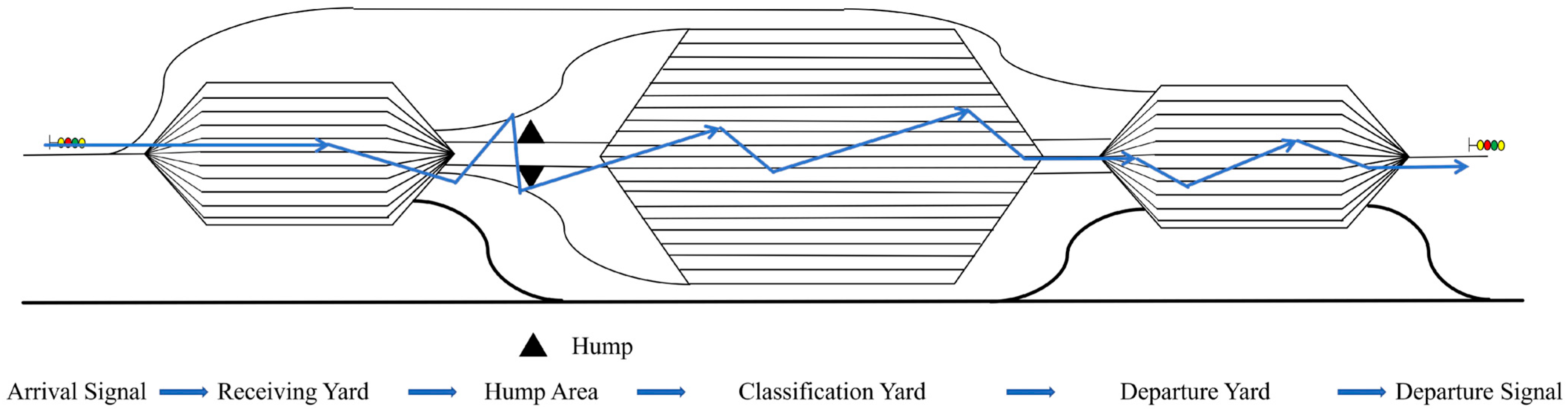
A typical marshalling yard consists of several functionally connected yards and operating facilities, including the receiving yard, hump, classification yard, and departure yard, as illustrated in Figure 1. After arriving at the yard, trains first enter the receiving yard, occupy arrival tracks, and undergo technical operations before being processed by hump disassembly. The marshalling yard inbound operations considered here refer to the arrival–technical-operation–hump-disassembly process.

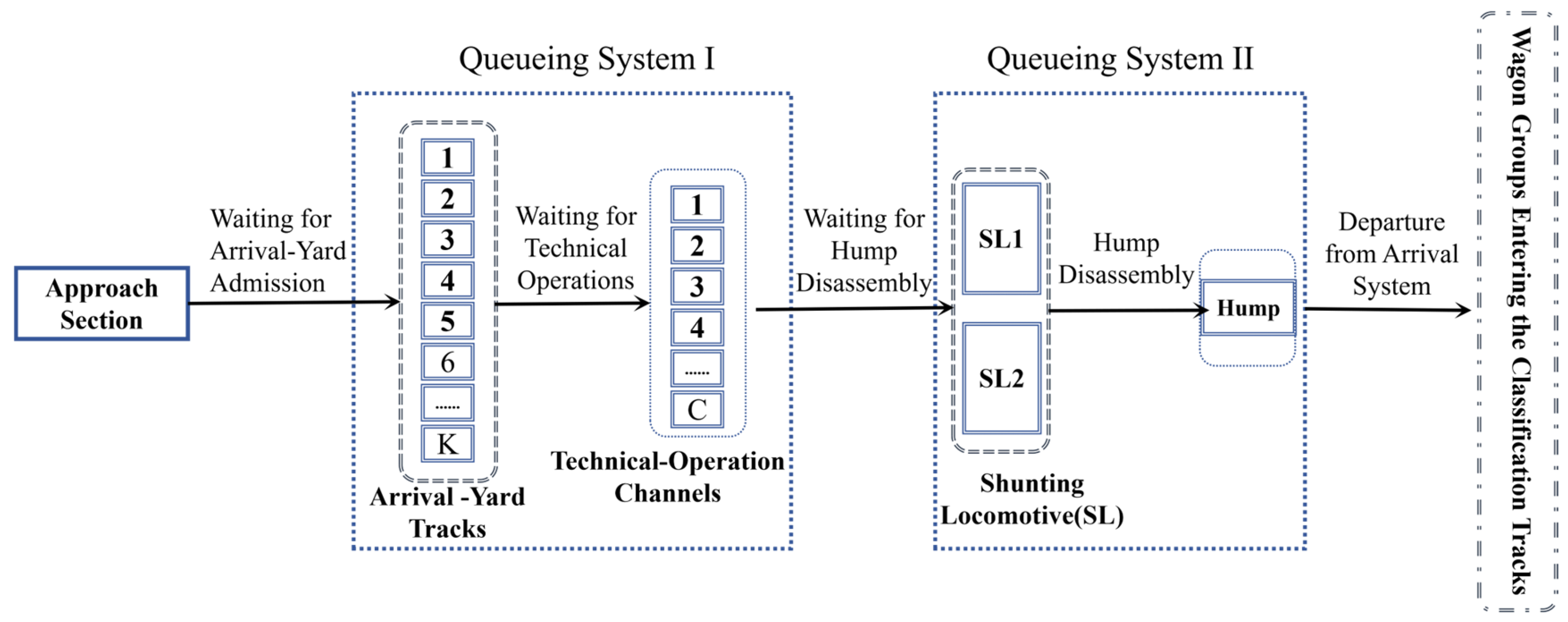
Based on this physical operating process, the arrival–operation subsystem considered in this study is abstracted as an arrival–technical-operation–hump-disassembly queueing system, as shown in Figure 2. Among these stages, hump disassembly is usually the key bottleneck where capacity constraints and congestion accumulation are most likely to occur [8].

Existing approaches to marshalling yard dispatching and capacity assessment often rely on fixed service times, static capacity assumptions, or experience-based rules. Although these methods are useful for conventional planning and operational evaluation, they provide limited support for explaining how congestion develops during continuous operation. In marshalling yard inbound operations, congestion may result from the combined effects of irregular train arrivals, finite receiving-yard capacity, time-varying clearance capacity, service-interruption windows, and residual states carried over from previous operating periods. When arrival fluctuations are not well matched with available processing capacity, trains may be delayed before entering the yard, leading to outside holding and reduced operational efficiency at the railway hub.

In this paper, we aim to develop a hybrid fluid–queueing and simulation framework for analyzing congestion evolution in the arrival–operation system of railway marshalling yards under irregular train arrivals. The framework represents stage-specific operating states, finite-capacity constraints, and time-varying service capacity along the arrival–technical-operation–hump-disassembly chain. It further validates long-term system stability under continuous operation, identifies residual-state propagation, and explains how internal queue accumulation spills over into outside holding.

The rest of this paper is organized as follows. Section 2 reviews related studies on marshalling yard operations, arrival variability, queueing models, and simulation-based risk analysis. Section 3 presents the modelling framework, including the multi-stage queueing formulation, periodic boundary steady-state validation (PSSBV), and daily gated integer discrete-event simulation (DGDES) procedure. Section 4 presents the case study and simulation results, including data description, input modelling, deterministic-service analysis, and stochastic-service Monte Carlo analysis. Section 5 summarizes the main conclusions and practical implications.

2. Literature Review

2.1. Train Management and Dispatching in Marshalling Yards

Marshalling yard management has traditionally focused on throughput capacity, waggon turnaround time, track and classification-line utilization, and operational deviations, and has gradually evolved from empirical rules and static capacity assessment toward dynamic rescheduling and real-time decision support for multi-stage, resource-constrained yard operations [9]. Based on North American classification-yard practice, Ref. [3] emphasized that bottleneck management is a key approach to improving terminal performance, indicating that marshalling yard capacity is often dominated by a limited number of critical processes. Ref. [10] summarized shunting-yard operations from both theoretical and practical perspectives, showing that marshalling yard dispatching has gradually developed into a research area supported by optimization, simulation, and rule-based control. Studies on hump-yard operational planning have shown that inbound train humping, car classification, outbound train formation, movement sequencing, and classification-track capacity constraints are closely related to waggon dwell time and yard operating performance [11,12]. Research has also emphasized dynamic rescheduling, resource coordination, and deviation management, with Ref. [8] showing that arrival delays, resource skill patterns, and resource rescheduling significantly affect overall classification-yard performance. Ref. [13] further demonstrates from a decision-support perspective that yard management under operational deviations and disturbances requires more real-time diagnostic and response mechanisms.

2.2. Arrival Variability and Irregularity

Arrival variability and uncertainty are important factors affecting marshalling yard performance, as uncertainty in the arrival process can significantly influence capacity utilization and delay levels in classification yards [14]. Ref. [15] further quantified, through simulation, the effects of classification-track length constraints and arrival variability on railway hump-yard capacity. Yard arrival prediction and operational deviation response studies further suggest that arrival rhythm, yard clearance capacity, and downstream train connections are closely coupled. Short-term arrival concentration, peak clustering, and residual queues from previous periods may therefore jointly contribute to congestion risk in yard operations [16,17].

In transportation systems, arrival irregularity is commonly described from two complementary perspectives: interval variability and count dispersion. The coefficient of variation in headways has been widely used in transport reliability studies to measure fluctuations in departure or arrival intervals, and related research has shown that headway irregularity is closely associated with service reliability and operational control performance [18,19,20]. In addition to interval-based measures, the dispersion of arrival counts within fixed time windows can be used to identify short-term traffic clustering. In point-process statistics, the index of dispersion for counts is commonly defined as the variance-to-mean ratio of arrival counts, and is used to assess whether a counting process is overdispersed or underdispersed relative to a Poisson benchmark [21,22]. In traffic-flow studies, vehicle-arrival variability has been characterized through the statistical properties of time headways, including the coefficient of variation in vehicle headways [23]. Arrival dispersion has also been expressed as the variance-to-mean ratio of arrival counts within fixed time intervals and incorporated into delay-related formulations [24].

2.3. Non-Stationary Queues and Fluid Approximations

The arrival–operation system examined in this paper involves non-stationary train arrivals, time-varying service capacity, finite-capacity blocking, and residual-state carryover during continuous operation. These characteristics make traditional steady-state queueing models insufficient for describing the dynamic evolution of queues and congestion. Non-stationary queueing models and fluid approximations therefore provide a useful theoretical basis for capturing time-dependent workload accumulation, bottleneck formation, and system-state evolution.

Ref. [25] developed a fluid model for multi-server queues under time-varying arrival and service conditions. Ref. [26] further extended time-varying multi-server fluid queues to network settings, providing a theoretical basis for analyzing time-dependent congestion in multi-stage serial–parallel systems. Fluid-limit analysis has also been extended to multiclass many-server queues with time-varying inputs and general reneging distributions, indicating that fluid approximations can be applied to more complex dynamic service systems [27].

For engineering-oriented approximations of non-stationary queues, Ref. [28] proposes the stationary backlog-carryover approach, which emphasizes the transfer of backlog across periods under temporary overload. This idea is closely related to the residual-queue propagation mechanism considered in marshalling yard operations, where unfinished workload at the boundary of one day may affect the congestion state of subsequent days. Refs. [29,30] provides practical methods for estimating non-stationary queueing performance from the perspectives of approximate modelling and staffing under time-varying demand. Studies on waiting-time and queue-length approximations under periodic or time-varying arrival rates have shown that robust approximations and fluid-based methods can characterize both average performance and periodic distributions in dynamic systems [31,32].

2.4. Discrete-Event Simulation, Analytical Modelling, and Risk Diagnosis

For systems involving complex operating rules, capacity blocking, and institutional service-window constraints, discrete-event simulation (DES) is an important tool for performance evaluation. DES can represent detailed event logic, resource occupation, queue evolution, and operational disruptions at the entity level. However, simulation alone often provides limited mechanistic explanation and may make it difficult to derive generalizable diagnostic indicators. From the perspective of simulation optimization, Refs. [33,34] note that combining simulation models with analytical approximations can improve the balance among operational realism, interpretability, and optimization capability.

In railway-yard applications, rule-based DES, AnyLogic-based yard simulation, and decision-support models for operational deviations and delays have been used to evaluate hump operations, yard clearance capacity, and operational risk [4,11,13]. At the same time, classical simulation methodology provides a foundation for defining performance indicators, designing stochastic experiments, and conducting robustness analysis in complex systems [35,36,37].

Overall, existing studies have advanced the analysis of marshalling yard operations and time-varying queueing systems. However, the continuous-operation evaluation of the arrival–technical-operation–hump-disassembly chain under irregular arrivals remains insufficiently addressed. In particular, arrival irregularity, finite-capacity blocking, service-interruption windows, and residual-state carryover have not been sufficiently integrated into a unified framework for explaining congestion evolution and identifying system risk.

3. Methodology

Based on the system abstraction introduced in Section 1 and established fluid–queueing, periodic-state, and discrete-event simulation principles, this section develops an application-specific methodological framework for analyzing congestion evolution in marshalling yard inbound operations. The section first formulates a fluid–queueing model to describe flow conservation and bottleneck formation. It then introduces a periodic boundary steady-state validation method to assess long-term stability and determine consistent initial states. Finally, a gated integer discrete-event simulation model is developed to simulate train-level operations under capacity limits and service-interruption constraints. The main notation and performance indicators used in the model are summarized in

Table 1. Nomenclature.

Notation	Description
$t$	Time within an operating day $t=0$ corresponds to 20:00
$T$	Length of an operating day $T=1440$min
$d$	Operating-day index
$\lambda \left(t\right)$	Non-stationary arrival intensity; trains/min; constructed by STEP or circular KDE
$A_d\left(t\right)$	Arrival count in minute $t$ of day $d;$ obtained from observed arrival data
$r_d\left(t\right)$	Fractional residual used when converting fluid arrivals into integer train arrivals
$C_Y$	Capacity of the receiving yard; $C_Y=12$ tracks in this study
$C_T$	Number of parallel technical-operation channels; $C_T=4$ in this study
$C_D$	Number of hump-disassembly servers; $C_D=1$ in this study
$S_T$	Technical-operation service time; observed mean value 36.57 min or random variable
$S_D$	Hump-disassembly service time; observed mean value 15.60 min or random variable
$u_T\left(t\right)$	Availability function of technical operations; $u_T\left(t\right)=1$ when available and 0 during shift-handover windows
$u_D\left(t\right)$	Availability function of hump disassembly; $u_D\left(t\right)=1$ when available and 0 during shift-handover and meal-break windows
${\eta }_T\left(t\right)$	Nominal processing capacity of the technical-operation stage; ${ \eta }_T\left(t\right)=C_T/S_T$ trains/min
${\eta }_D\left(t\right)$	Nominal processing capacity of the hump-disassembly stage; ${ \eta }_D\left(t\right)=C_D/S_D$ trains/min
$E_T$	Nominal daily capacity of technical operations; $E_T={\int }_0^T{u}_T\left(t\right)·{\eta }_T\left(t\right)dt=150.9$ trains/day
$E_D$	Nominal daily capacity of hump disassembly; $E_D={\int }_0^T{u}_D\left(t\right)·{\eta }_D\left(t\right)dt=84.6$ trains/day
$Q_{out}\left(t\right)$	Outside holding queue length at time $t;$ FIFO discipline
$Q_T\left(t\right)$	Work-in-process in the technical-operation stage, including waiting and in-service trains
$Q_{sT}\left(t\right)$	Number of trains in technical service at time $t$
$Q_D\left(t\right)$	Work-in-process in the disassembly stage, including waiting and in-service trains
$Q_{sD}\left(t\right)$	Number of trains in disassembly service at time $t$
$Q_{arr}\left(t\right)$	Total in-yard occupancy at time $t$
$Q_{wT}\left(t\right)$	Technical waiting queue length at time $t$
$Q_{wD}\left(t\right)$	Disassembly waiting queue length at time $t$
$I\left(t\right)$	Remaining processing-time vector of technical-operation and disassembly channels; $I\left(t\right)=\left(i_1\left(t\right),...,i_{C_{\mathcal{I}}}\left(t\right),i_{C_{\mathcal{D}}}\left(t\right)\right)$
$x_d$	Boundary state at the beginning of day $d,$ including queues, service states, remaining processing times, and fractional residuals
$F(·)$	One-day boundary-state evolution operator; $x_{d+1}=F\left(x_d\right)$
${CV}_{IA}$	Coefficient of variation in inter-arrival times
${Fano}_w$	Fano factor under window length $w;$ used to measure arrival clustering over fixed time windows
$N_{arr}\left(d\right)$	Total arrivals on day $d,$ including admitted and outside-held trains
$N_{dep}\left(d\right)$	Throughput on day $d,$ defined as the number of trains completing hump disassembly
$N_T^{star}\left(d\right)$	Number of trains starting technical service on day $d;$ used in Little-type calculations
$N_D^{star}\left(d\right)$	Number of trains starting disassembly service on day $d;$ used in Little-type calculations
$N_{out}\left(d\right)$	Number of trains entering outside holding on day $d$
${\overline{Q}}_{arr}^{\left(d\right)}$	Average in-yard occupancy on day $d;$ ${\overline{Q}}_{arr}^{\left(d\right)}=A_{arr}\left(d\right)/T$
$R_{out}\left(d\right)$	Outside holding rate on day $d;$ $R_{out}\left(d\right)=N_{out}\left(d\right)/N_{arr}\left(d\right)$
$W_{out}\left(d\right)$	Mean outside waiting time on day $d;$ $W_{out}\left(d\right)=A_{out}\left(d\right)/N_{out}\left(d\right)$ min
$W_{qT}\left(d\right)$	Mean technical waiting time on day $d;$ $W_{qT}\left(d\right)=A_{wT}\left(d\right)/N_T^{start}\left(d\right)$ min
$W_{qD}\left(d\right)$	Mean disassembly waiting time on day $d;$ $W_{qD}\left(d\right)=A_{wD}\left(d\right)/N_D^{start}\left(d\right)$ min
$W_{sys}\left(d\right)$	Mean system sojourn time on day $d;$ $W_{sys}\left(d\right)=A_{arr}\left(d\right)/N_{dep}\left(d\right)$ min
$A_{arr}\left(d\right)$	Cumulative area of total in-yard occupancy on day $d;$ $A_{arr}\left(d\right)={\int }_0^T{Q}_{arr}^{\left(d\right)}\left(t\right)dt$ train·min
$A_{out}\left(d\right)$	Cumulative area of the outside holding queue on day $d;$ $A_{out}\left(d\right)={\int }_0^T{Q}_{out}^{\left(d\right)}\left(t\right)dt$ train·min
$A_{wT}\left(d\right)$	Cumulative area of the technical waiting queue on day $d;$ $A_{wT}\left(d\right)={\int }_0^T{Q}_{wT}^{\left(d\right)}\left(t\right)dt$ train·min
$A_{wD}\left(d\right)$	Cumulative area of the disassembly waiting queue on day $d;$ $A_{wD}\left(d\right)={\int }_0^T{Q}_{wD}^{\left(d\right)}\left(t\right)dt$ train·min

.

3.1. Flow Conservation, Blocking, and Time-Varying Capacity Under Service Interruptions

3.1.1. Construction of the Fluid Arrival Process

The train arrival process at a marshalling yard is jointly affected by real-time dispatching decisions, section capacity, operational coordination with upstream and downstream stations, and temporary transportation adjustments. Therefore, it generally does not satisfy the assumptions of a stationary Poisson process or identically distributed arrivals. This non-stationary feature is further confirmed by the empirical analysis in Section 4. Accordingly, a time-varying arrival intensity function, λ(t), is used to represent the arrival process and to characterize the non-stationary input load under realistic dispatching conditions.

To preserve the descriptive capability of a continuous arrival-rate function while maintaining the discrete entity nature of trains, this paper adopts a “residual accumulation–integer conversion” mechanism to transform the continuous arrival flow into integer train arrivals. Under a discrete time step $\mathsf{\Delta }t$, the expected number of arrivals in each time step, $\lambda \left(t\right)\mathsf{\Delta }t$, is calculated and accumulated in a residual variable. When the accumulated residual $r_d\left(t\right)$ reaches or exceeds one, the corresponding integer number of train arrivals is generated; the generated integer part is then subtracted from the residual, and the remaining fractional part is carried over to the next time step. The mechanism is expressed in Equations (1)–(3), where $\lfloor \cdot \rfloor$ denotes the floor operator.

$$r_d(t+\mathsf{\Delta }t)=r_d\left(t\right)+\lambda \left(t\right)\mathsf{\Delta }t$$

(1)

$${\mathit{A}}_{\mathit{d}}(\mathit{t})=\lfloor {\mathit{r}}_{\mathit{d}}\left(\mathit{t}+\mathsf{\Delta }\mathit{t}\right)\rfloor$$

(2)

$$r_d(t+\mathsf{\Delta }t)\leftarrow {\mathit{r}}_{\mathit{d}}\left(\mathit{t}+\mathsf{\Delta }\mathit{t}\right)-{\mathit{A}}_{\mathit{d}}\left(\mathit{t}\right)$$

(3)

The choice of $\mathsf{\Delta }t$ affects how the continuous arrival intensity is converted into integer train arrivals, and its influence on the baseline simulation results should therefore be assessed through sensitivity analysis. Meanwhile, $\mathsf{\Delta }t$ should not be excessively large, because $\lambda \left(t\right)\mathsf{\Delta }t$ may exceed one during high-intensity periods and may cause two train arrivals to be generated at the same time through residual accumulation. This is inconsistent with the train-by-train arrival and admission process in actual yard operations. This mechanism avoids directly feeding continuous fluid quantities into the queueing system, which would otherwise violate the discreteness of train entities. At the same time, it preserves the intraday time-varying structure of the arrival intensity, thereby providing a consistent input basis for the subsequent unified modelling framework.

3.1.2. Flow Conservation and Two-Stage Fluid Equations

(1) Flow conservation

After admission to the arrival yard, trains remain within the in-yard system until hump disassembly is completed. The total in-yard occupancy is given by the sum of the technical-operation-stage content and the disassembly stage content as in Equation (4).

$$Q_{arr}\left(t\right)=Q_T\left(t\right)+Q_D\left(t\right)$$

(4)

When $Q_{arr}\left(t\right)$ reaches the arrival-yard capacity ${\mathit{C}}_{\mathit{Y}}$, additional arriving trains cannot be admitted immediately and are assigned to the outside holding queue ${\mathit{Q}}_{\mathit{out}}\left(\mathit{t}\right)$ under the FIFO rule. This relationship reflects the flow-conservation structure of the arrival–operation system.

(2) Two-stage fluid equations

Let ${\mathit{\varphi }}_{\mathit{T}}\left(\mathit{t}\right)$ and ${\mathit{\varphi }}_{\mathit{D}}\left(\mathit{t}\right)$ denote the completion flow rate of the technical-operation stage and the outflow rate of the hump-disassembly stage, respectively. The fluid approximation of the two-stage arrival–operation system is formulated as follows:

$${\displaystyle \frac{\mathit{d}{\mathit{Q}}_{\mathit{T}}(\mathit{t})}{\mathit{dt}}}={\mathit{\lambda }}_{\mathit{in}}(\mathit{t})-{\mathit{\varphi }}_{\mathit{T}}(\mathit{t})$$

(5)

$${\displaystyle \frac{\mathit{d}{\mathit{Q}}_{\mathit{D}}(\mathit{t})}{\mathit{dt}}}={\mathit{\varphi }}_{\mathit{T}}(\mathit{t})-{\mathit{\varphi }}_{\mathit{D}}(\mathit{t})$$

(6)

$${\mathit{\varphi }}_{\mathit{T}}(\mathit{t})=\min \left\{{\mathit{\mu }}_{\mathit{T}}\left(\mathit{t})·{\mathit{\eta }}_{\mathit{T}}\right(\mathit{t}),{ \mathit{Q}}_{\mathit{T}}\left(\mathit{t}\right)\right\}$$

(7)

$${\mathit{\varphi }}_{\mathit{D}}(\mathit{t})=\min \left\{{\mathit{\mu }}_{\mathit{D}}\left(\mathit{t})·{\mathit{\eta }}_{\mathit{D}}\right(\mathit{t}),{ \mathit{Q}}_{\mathit{D}}\left(\mathit{t}\right)\right\}$$

(8)

$${\mathit{\lambda }}_{\mathit{in}}\left(\mathit{t})=\mathit{\lambda }\right(\mathit{t})·1\left\{{\mathit{Q}}_{\mathit{arr}}(\mathit{t})<{\mathit{C}}_{\mathit{Y}}\right\}$$

(9)

Equation (5) describes the evolution of the fluid content in the technical-operation stage as the difference between the effective inflow rate ${\mathit{\lambda }}_{\mathit{in}}\left(\mathit{t}\right)$ and the technical completion rate ${\mathit{\varphi }}_{\mathit{T}}\left(\mathit{t}\right)$.

Equation (6) describes the evolution of the disassembly stage fluid content as the difference between the inflow from the technical stage ${\mathit{\varphi }}_{\mathit{T}}\left(\mathit{t}\right)$ and the disassembly outflow rate ${\mathit{\varphi }}_{\mathit{D}}\left(\mathit{t}\right)$.

Equations (7) and (8) specify the actual processing rates of the technical-operation and hump-disassembly stages as the minimum between the available service capacity and the current fluid content, while incorporating the effects of shift handovers, meal breaks, and other service-interruption windows on time-varying service capacity.

Equation (9) defines $1\left\{{\mathit{Q}}_{\mathit{arr}}(\mathit{t}) <{ \mathit{C}}_{\mathit{Y}}\right\}$ as an indicator function describing whether the arrival yard has available capacity. When ${\mathit{Q}}_{\mathit{arr}}(\mathit{t}) <{ \mathit{C}}_{\mathit{Y}}$, arriving trains can enter the yard and ${\mathit{\lambda }}_{\mathit{in}}\left(\mathit{t}) = \mathit{\lambda }\right(\mathit{t})$. Otherwise, the effective inflow into the yard becomes zero, and newly arriving trains are held outside the yard.

3.2. Steady-State Validation and Arrival-Irregularity Diagnosis

3.2.1. Long-Term Stability and Periodic Steady State

For the marshalling yard arrival–operation system, long-term behaviour should be evaluated not only by instantaneous congestion levels but also by whether the system remains bounded over successive operating days. The system state at the daily boundary is used to characterize residual conditions carried over to the next operating day, and the one-day evolution from operating day $\mathit{d}$ to operating day $\mathit{d} + 1$ can be expressed as Equation (10):

$$x_{d+1}=F\left(x_d\right)$$

(10)

If there exists a boundary state $x^{\mathrm{*}}$ satisfying:

$$F\left(x^{\mathrm{*}}\right)=x^{\mathrm{*}}$$

(11)

then the system reaches a fixed-point state at the daily scale. If there exists a period length $\mathit{L}$ satisfying:

$$F^{\left(L\right)}\left(x^{*}\right)=x^{*}$$

(12)

then the system follows a periodic trajectory with period $\mathit{L}$.

For marshalling yard operations, a fixed point or periodic boundary trajectory does not imply the absence of queueing within an operating day. Rather, it indicates that residual queues and unfinished workloads remain bounded across successive days, so that the system can maintain long-term operational stability. Conversely, if outside holding, in-yard occupancy, or remaining workload continues to increase over consecutive days, the arrival pattern is not well matched with the available service capacity, and the system can be regarded as overloaded or unstable.

3.2.2. Arrival-Irregularity Metrics

(1) Coefficient of variation in inter-arrival times ($C{V}_{IA}$)

The indicator $\mathit{C}{\mathit{V}}_{\mathit{IA}}$ measures the dispersion of inter-arrival times. Let ${\mathsf{\Delta }}_{\mathit{i}}$ denote the sequence of inter-arrival times between adjacent trains on operating day $d$. The $\mathit{C}{\mathit{V}}_{\mathit{IA}}$ is defined in Equation (13):

$$C{V}_{IA}(d)={\displaystyle \frac{std\left({\mathsf{\Delta }}_i\right)}{mean\left({\mathsf{\Delta }}_i\right)}}$$

(13)

where $std\left({\mathsf{\Delta }}_i\right)$ and $mean\left({\mathsf{\Delta }}_i\right)$ are the standard deviation and mean of the inter-arrival-time sequence, respectively. A larger $C{V}_{IA}$ indicates stronger fluctuation in arrival rhythm and less regular arrival spacing, whereas a smaller $C{V}_{IA}$ suggests a more stable arrival process closer to uniform arrivals.

(2) Fano factor ($Fan{o}_w$)

To further measure the clustering of arrival counts within fixed time windows, each operating day is divided into equal-length windows. In this study, the window length $\mathrm{w}$ is set to 30 min. Let $N_j$ denote the number of train arrivals in the $j$-th time window of operating day, where $j=1,2,\dots ,J$, and $J=1440/w$. The Fano factor is defined in Equation (14):

$$Fan{o}_w(d)={\displaystyle \frac{Var\left(N_j\right)}{E\left(N_j\right)}}$$

(14)

where $var\left(N_j\right)$ and $E\left(N_j\right)$ denote the variance and mean of arrival counts across all time windows, respectively. When $Fan{o}_w>1$, the arrival process exhibits overdispersion and evident clustering. When $Fan{o}_w\approx 1$, the arrival-count fluctuation is close to that of a Poisson arrival process. When $Fan{o}_w<1$, the arrivals are relatively more evenly distributed across time windows.

3.2.3. Periodic Boundary Steady-State Validation (PSSBV) Algorithm

To avoid the bias introduced by arbitrary initial boundary conditions in simulations over consecutive operating days and to assess whether the system can sustain long-term operation under given arrival inputs and service-capacity settings, this study incorporates the initial state of each operating day into the boundary-state representation. This boundary state captures cross-day residual conditions, including queues, service states, remaining processing times, and unfinished workloads carried over from the previous day. Based on this representation, a periodic boundary steady-state validation algorithm (PSSBV) is developed, and its detailed procedure is shown in

Table 2. Specific steps of the PSSBV algorithm.

Step	Processing and Calculation Steps
Initialization.	Set $k=0;$ specify the tolerance $\epsilon ;$ the maximum number of iterations $K_{\mathrm{m}\mathrm{a}\mathrm{x}};$ the maximum period length $L_{\mathrm{m}\mathrm{a}\mathrm{x}};$ define the historical boundary-state set as $H=\left\{x_0\right\}.$
Arrival-input processing	For $\lambda \left(t\right),$ determine the arithmetic residual-phase length $L_r.$ For $A_d\left(t\right),$ set $L_r=1.$
Daily state mapping	Run a one-day simulation under the given arrival input, service-capacity settings, service-interruption windows, and operating rules, and update the boundary state as $x_{k+1}=F\left(x_k\right).$
Fixed-point identification	If the fixed-point residual satisfies $Re{s}^k=\Vert x_{k+1}-x_k\Vert \le \epsilon ,$ then output the fixed-point boundary state $x^{*}=x_k,$ and terminate the algorithm.
Periodic-state identification	For $L=2,\dots ,L_{max},$ if there exists a period length $L$ such that $Re{s}^k=\Vert x_{k+1}-x_k\Vert \le \epsilon ,$ then output the periodic trajectory with period $L;$ if $L_r=1,$ terminate the algorithm.
Phase-matched comparison	For $L_r>1,$ examine phase-compatible candidate lengths $L={mL}_r,$ where $m=1, 2,\dots ,\lfloor L_{max}/L_r\rfloor .$ If $k+1\ge L$ and $Re{s}^{k,L}=\Vert x_{k+1}-x_{k+1-L}\Vert \le \epsilon ,$ output the boundary-state trajectory with recurrence length $L$ and terminate the algorithm.
Stability diagnosis	If the boundary state continues to increase, exceeds the predefined stability range, or no fixed point or periodic trajectory is identified when $k=K_{max},$ the system is classified as unstable or overloaded. Otherwise, update $k\leftarrow k+1,$ add $x_{k+1}$ to the historical state set $H,$ and return to daily state mapping.

.

It should be noted that the treatment of the arrival residual depends on the input representation. When $\lambda \left(t\right)$ input is used, the arrival residual $r_d\left(t\right)$ is updated across time steps and transferred across operating-day boundaries, and is included in the boundary-state comparison. Cross-day residual accumulation may cause some operating days to generate one additional whole train. Therefore, even when the same continuous daily arrival–intensity profile is repeatedly applied, the integer train-arrival events entering the daily state mapping $x_{k+1}=F\left(x_k\right)$ may pass through different residual phases.

Let the mean daily arrival volume be

$$\overline{N}=q+{\displaystyle \frac{a}{b}}$$

(15)

where $q$ is the integer part and $\mathrm{a}/\mathrm{b}$ is the fractional part expressed in lowest terms, representing the initial arrival residual $r_d\left(t\right)$ transferred across operating-day boundaries. The arrival residual returns to the same arithmetic phase after $b$ daily iterations; therefore, the arithmetic phase length is

$$L_r=b$$

(16)

For the $A_d\left(t\right)$ sequence, trains enter the daily mapping directly according to their specified arrival times. In this case, $r_d\left(t\right)$ is neither updated nor transferred. It therefore has no effect on the boundary-state residual calculation. For unified implementation, the discrete-input case can be regarded as having phase, equivalently

$$L_r=1$$

(17)

Therefore, given the arithmetic phase length ${\mathrm{L}}_{\mathrm{r}}$, the main role of PSSBV is to verify whether the operational boundary state returns after one or more complete residual-phase cycles while remaining bounded, and output the corresponding nonzero initial boundary state.

3.3. Gated Integer Discrete-Event Simulation Model

3.3.1. State Variables, Event Mechanism, and Train-Entity Control Rules

(1) State variables

To describe the discrete operation process of the “arrival–technical-operation–disassembly” system, three types of core state variables are defined in the simulation: queue states, service states, and aggregate system states. The queue states include outside holding $Q_{out}\left(t\right)$, technical-operation waiting $Q_{wT}\left(t\right)$, and disassembly waiting $Q_{wD}\left(t\right)$. The service states record the numbers of trains undergoing technical operations $Q_{sT}\left(t\right)$ and hump disassembly $Q_{sD}\left(t\right)$, which are constrained by the technical-operation capacity $C_T$ and the disassembly capacity ${\mathit{C}}_{\mathit{D}}$, respectively. During service-interruption windows, trains already in service continue to occupy their assigned resources, and the remaining processing-time vector $I\left(t\right)$ is retained until service becomes available again. The aggregate system state is represented by the total in-yard occupancy $Q_{arr}\left(t\right)$, which measures the number of trains occupying receiving-yard resources. It can be expressed as the sum of trains waiting for and undergoing technical operations and hump disassembly:

$$Q_{arr}\left(t\right)=Q_T\left(t\right)+Q_D\left(t\right)=\left(Q_{wT}\left(t\right)+Q_{sT}\left(t\right)\right)+\left(Q_{wD}\left(t\right)+Q_{sD}\left(t\right)\right)$$

(18)

In addition, the model records the arrival residual $r_d\left(t\right)$ and the entry timestamps of trains in the outside holding queue $Q_{out}\left(t\right)$, which are used to calculate waiting times, cross-day residual states, and boundary-state updates.

(2) Key discrete events

The main discrete events in the simulation are defined as follows,

Arrival event. When an arriving train is waiting for admission, the model first checks the available capacity of the receiving tracks. If the yard is not full, the train enters the technical-operation waiting queue; otherwise, it joins the outside holding queue.

Outside-to-yard admission event. When in-yard occupancy is released and the outside holding queue is nonempty, the earliest waiting train is admitted into the yard according to the FIFO rule.

Technical-operation start event. If the technical waiting queue is nonempty, at least one technical channel is idle, and the system is within an available technical-operation period, that is, $u_T\left(t\right)=1$, the train starts technical service.

Technical-operation completion event. When the remaining processing time of a technical operation reaches zero, the train leaves the technical service state and enters the disassembly waiting queue.

Disassembly start event. If the disassembly waiting queue is nonempty, the disassembly resource is idle, and the system is within an available disassembly period, that is, $u_D\left(t\right)=1$, the train starts disassembly service.

Disassembly completion event. When the remaining disassembly processing time reaches zero, the train leaves the arrival system, releases the disassembly resource, and releases the corresponding in-yard occupancy.

(3) Train-Entity Control Rules

The gated train-entity control rule is a key feature of the gated integer discrete-event simulation model (DGDES), distinguishing it from both purely continuous queueing approximations and conventional aggregate discrete queueing models. In this study, “gated whole-train service” means that each train occupies and releases resources as an indivisible operational unit. In the stochastic-service simulation, each train is assigned an independently sampled technical-operation and hump-disassembly service time. Once a train starts technical service or hump disassembly, it continuously occupies the corresponding service resource until the operation is completed. If a service-interruption window occurs during this period, the train remains in service and the occupied resource cannot be assigned to another train. The release of in-yard occupancy is also gated. A train releases its occupied arrival track only after hump disassembly is completed and the train leaves the arrival system.

3.3.2. Simulation Procedure and Output Indicators

Based on the state definitions and event rules described above, the detailed DGDES steps are shown in

Table 3. The detailed steps of the DGDES procedure.

Step	Specific Contents
Step 1	Initialization. For operating day $\mathrm{d},$ specify the system parameters $c_T$ and $c_D,$ service-time settings $S_T$ and $S_D,$ service-interruption windows, and the initial boundary state $x_d.$ The statistical variables are then initialized, including, $A_{wT},$ $A_{wD},$ $A_{arr},$ $A_{out},$ $N_{arr},$ $N_{out},$ $N_T^{start},$ $N_D^{start},$ $N_{dep}.$
Step 2	Arrival and admission decision. At each time step, arrivals are generated according to $\lambda \left(t\right),$ or the empirical arrival sequence $A_d\left(t\right).$ The arrival residual $r_d\left(t\right)$ is updated when the intensity-based input is used. If ${Q_{arr}\left(t\right)<C}_Y,$ the arriving train is admitted to the receiving yard and added to the technical waiting queue $Q_{wT}\left(t\right);$ otherwise, it joins the outside holding queue $Q_{out}\left(t\right).$
Step 3	Outside-to-yard FIFO admission When capacity becomes available in the arrival yard and $Q_{out}\left(t\right)\ge 1,$ the earliest waiting train in the outside holding queue is admitted according to the FIFO rule.
Step 4	Service availability judgement. The service availability functions $u_T\left(t\right)$ and $u_D\left(t\right)$ are updated according to the predefined shift-handover and meal-break windows.
Step 5	Technical-operation progression. For the technical-operation stage, trains can start service only when $Q_{wT}\left(t\right)\ge 1,$ $Q_{sT}\left(t\right)<C_T$ and $u_T\left(t\right)=1.$ The number of trains starting technical service at time $t$ is defined as $b_T\left(t\right)=\mathrm{m}\mathrm{i}\mathrm{n}\left\{Q_{wT}\right(t),C_T-Q_{sT}(t\left)\right\}{1}_{\left\{u_T\right(t)=1\}}$ Accordingly, $Q_{wT}\left(t\right)$ decreases by $b_T\left(t\right),$ $Q_{st}\left(t\right)$ increases by $b_T\left(t\right),$ and $N_T^{start}\left(d\right)$ is updated. For trains in technical service, the remaining processing time $I_T\left(t\right)$ decreases only during available service periods, i.e., $I_T(t+∆t)=I_T\left(t\right)-u_T\left(t\right)∆t.$ Once $I_T\left(t\right)\le 0,$ the train leaves $Q_{sT}\left(t\right)$ and joins $Q_{wD}\left(t\right).$
Step 6	Disassembly progression. For the hump-disassembly stage, trains can start service only when $Q_{wD}\left(t\right)\ge 1,$ $Q_{sD}\left(t\right)<C_D$ and $u_D\left(t\right)=1.$ The number of trains starting disassembly service at time $\mathrm{t}$ is given by $b_D\left(t\right)=\mathrm{m}\mathrm{i}\mathrm{n}\left\{Q_{wD}\right(t),C_D-Q_{sD}(t\left)\right\}{1}_{\left\{u_D\right(t)=1\}}.$ Accordingly, $Q_{wD}\left(t\right)$ decreases by $b_D\left(t\right),$ $Q_{sD}\left(t\right)$ increases by $b_D\left(t\right),$ and $N_D^{start}\left(d\right)$ is updated. For trains in disassembly service, the remaining processing time $I_D\left(t\right)$ decreases only during available disassembly periods, i.e., $I_D(t+∆t)=I_D\left(t\right)-u_D\left(t\right)∆t.$ Once $I_D\left(t\right)\le 0,$ the train leaves $Q_{sD}\left(t\right),$ $N_{dep}\left(d\right)$ increases by one, and the corresponding in-yard occupancy $Q_{arr}\left(t\right)$ is released.
Step 7	Statistical output. At the end of the operating day, the model outputs the daily performance indicators, including cumulative queue and occupancy areas $A_{wT},$ $A_{wD},$ $A_{arr},$ and $A_{out};$ average waiting and sojourn times $W_{qT}\left(d\right),$ $W_{qD}\left(d\right)$ and $W_{sys}\left(d\right);$ count indicators $N_{arr},$ $N_{out},$ and $N_{dep};$ diagnostic indicators $C{V}_{IA}\left(d\right),$ ${Fano}_w\left(d\right),$ ${\overline{Q}}_{arr}^{\left(d\right)},$ and $R_{out}\left(d\right);$ and the next-day boundary state $x_{d+1}.$

.

Waiting times and system sojourn time are calculated using an area-to-count accounting scheme consistent with Little’s law [38]. The detailed calculation methods for these indicators are summarized in Table 1. The monthly means of $R_{out}\left(d\right)$, $W_{out}\left(d\right)$, and $A_{out}\left(d\right)$ are calculated as arithmetic means over all operating days in the monthly sample. Zero-event days are retained: $R_{out}\left(d\right)=0$ when no train enters outside holding, $W_{out}\left(d\right)=0$ when no train is released from the outside FIFO queue, and $A_{out}\left(d\right)=0$ when the outside queue remains empty. Therefore, ${\overline{W}}_{out}$ is an unconditional daily mean rather than an average restricted to days with outside holding.

4. Case Study and Results

4.1. Data Description and Input Modelling

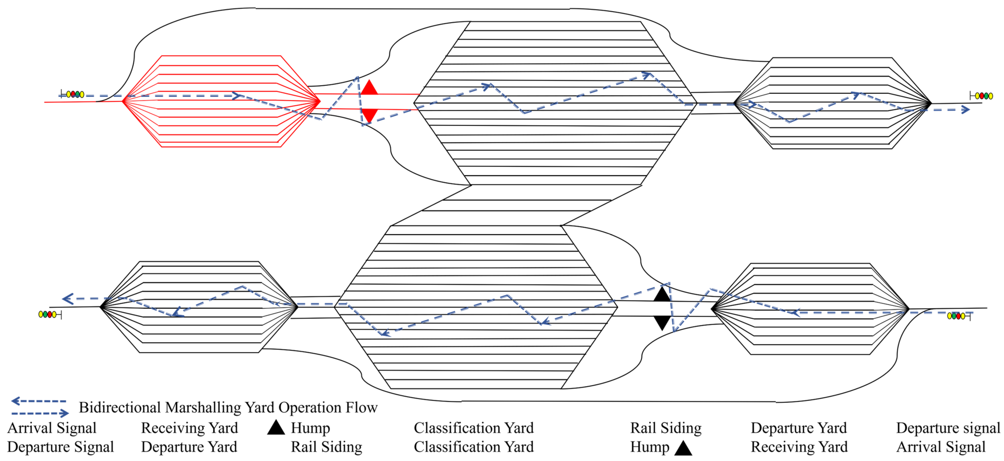
The simulation experiments are based on field data from the up-direction arrival–operation subsystem of a large network-level marshalling yard in western China. The yard has a three-level, seven-yard physical layout, and the study scope corresponds to the up-direction arrival subsystem highlighted in red in Figure 3. This subsystem includes train arrival, technical operations in the receiving yard, and hump disassembly. The dataset contains complete train arrival timestamps over consecutive operating days, together with train-level service-time records for both technical operations and hump disassembly.

Although the case-study yard has a complex physical layout, the hump-disassembly stage is represented as a single effective server in the DGDES model, with the hump service capacity set as $C_D=1$. This abstraction is consistent with the yard’s actual double-push and single-release operating mode, in which only one train can occupy the hump-release process at a time within each directional system.

The main empirical sample covers 31 consecutive operating days in January 2024. According to the timetable-adjustment practice of Chinese railways, January is usually the early stage after the implementation of a new-train working diagram, when operational uncertainty is relatively high. It also overlaps with the Spring Festival travel peak period, making January a relevant high-pressure case month. To examine cross-month consistency, the March 2024 dataset within the same timetable-adjustment period is further introduced as a comparison sample, when operations are relatively more stable after a period of adaptation. In accordance with the station’s shift-handover arrangement, 20:00 is defined as the starting point of each operating day. All arrival timestamps are converted into accumulated minutes from 20:00 on the first operating day to construct a continuous operational time series.

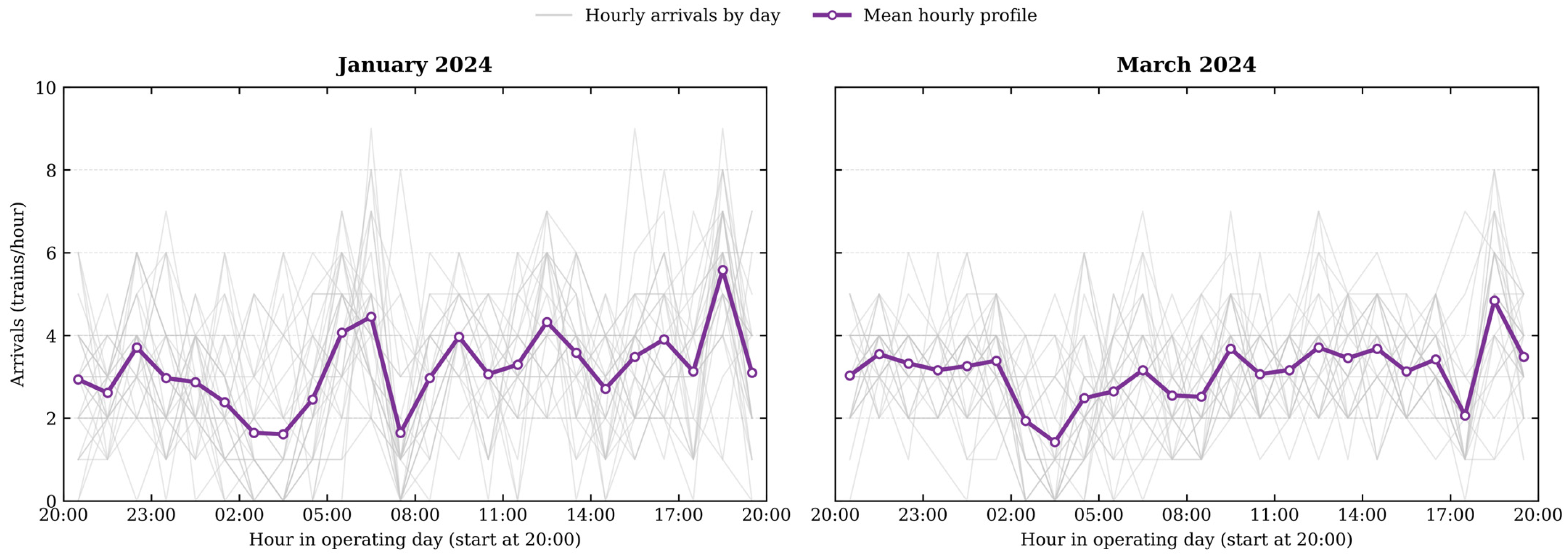
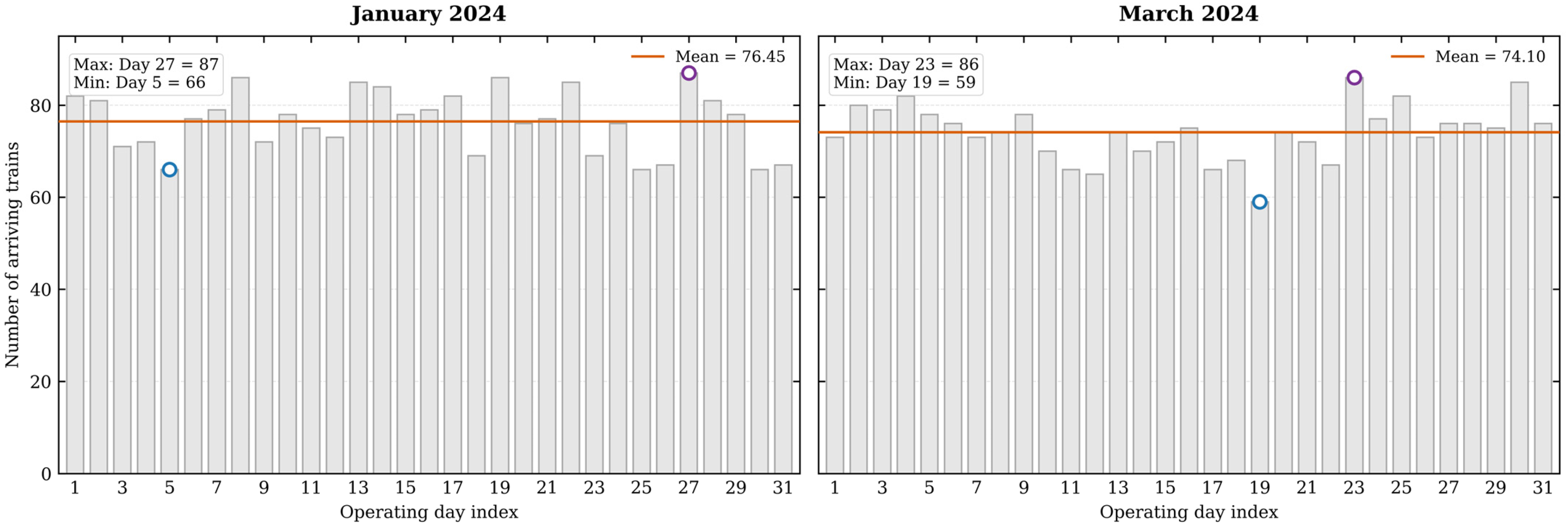
Figure 4 compares the hourly arrival patterns and mean hourly profiles for January and March, showing the intraday variation in train arrivals in the two months. Figure 5 presents the daily total arrivals for the corresponding operating days, further illustrating the cross-day fluctuation in arrival volume.

Two types of arrival inputs are used in the experiments. The first is the baseline-day average arrival intensity, $\lambda \left(t\right)$, which is used for periodic boundary steady-state validation. The second is the empirical daily arrival sequence, $A_d\left(t\right)$, used for continuous-operation simulation under observed input disturbances.

(1) Construction of the Baseline-Day Arrival-Rate Function

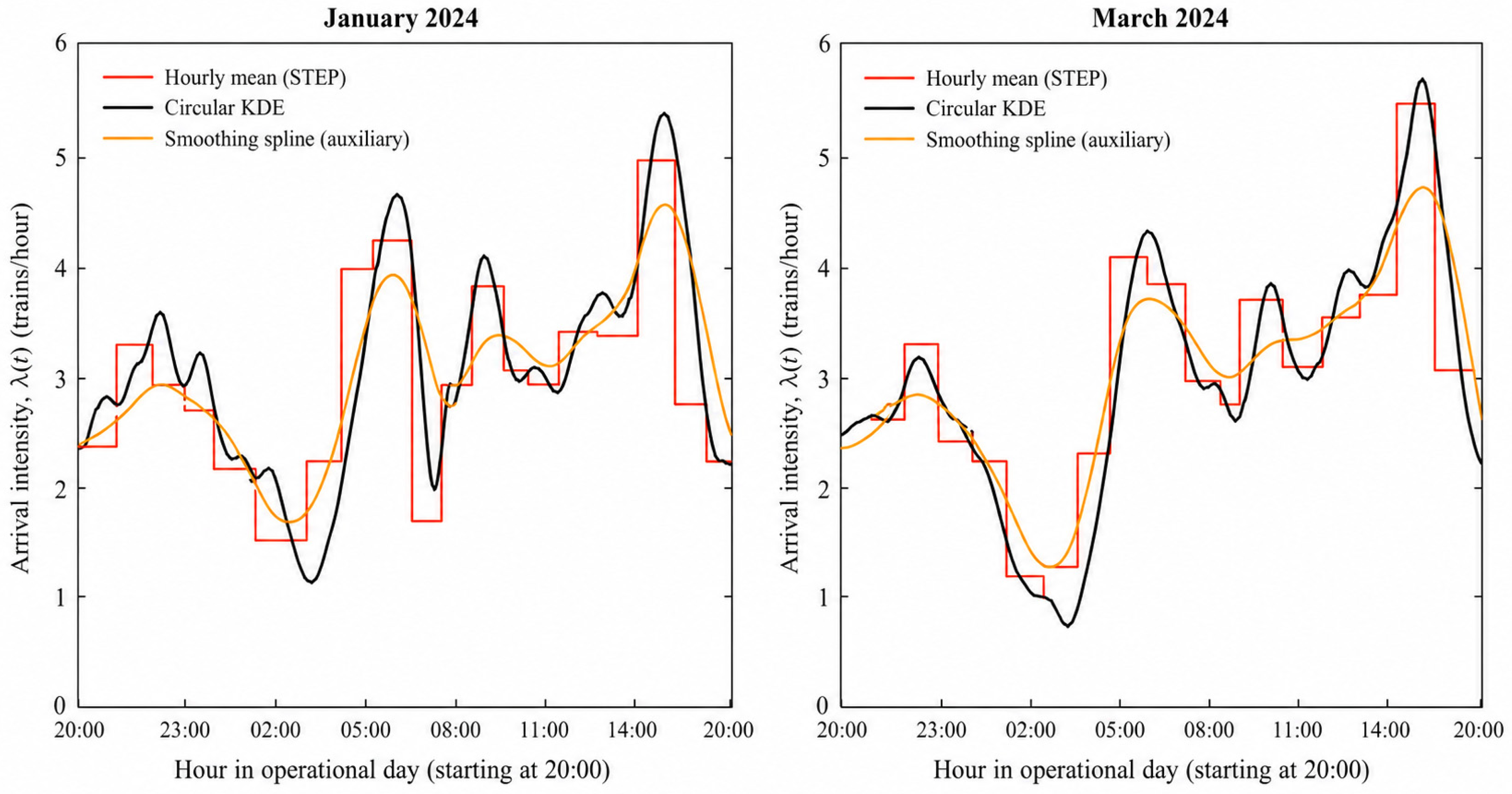
For the baseline-day arrival input, this study uses STEP and circular kernel density estimation (KDE) to construct the arrival-rate function, with a smoothing spline included for comparison, as shown in Figure 6.

The STEP method constructs a piecewise-constant arrival intensity from the mean hourly arrival counts over all operating days in each monthly sample, thereby preserving the hourly peak–valley structure of the arrival process. By contrast, circular KDE estimates a continuous non-stationary arrival-rate function from train arrival times on a minute-level grid [39]. Since each operating day starts at 20:00, historical arrival times are first converted into intraday times ${\mathrm{t}}_{\mathrm{i}}\in [0,T)$, where $T=1440$ min. The circular KDE intensity is then formulated as in Equation (19):

$${\lambda }_{KDE}(t)={\displaystyle \frac{{\overline{N}}_{arr}}{n}}{\sum }_{i=1}^n{\sum }_{m=-M}^M{\displaystyle \frac{1}{h\sqrt{2\pi }}}{e}^{{\left(-\left(t-t_i+m·T\right)\right)}^2/2h^2}$$

(19)

where ${\overline{N}}_{arr}$ is the mean daily number of arrivals, $n$ denotes the total number of pooled arrival samples in each monthly dataset, rather than the number of operating days, and $M$ is the truncation order of the periodic extension.

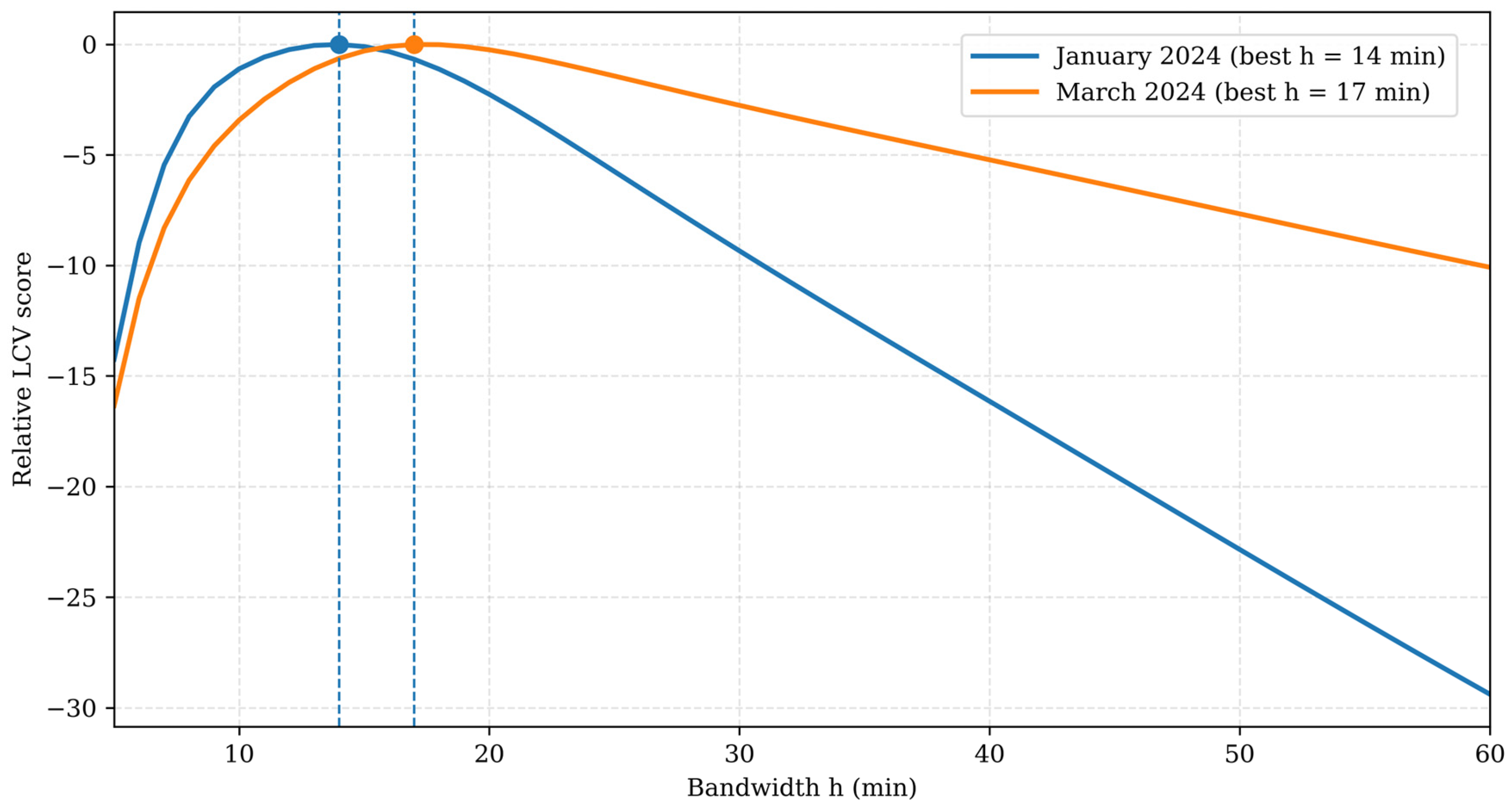
The bandwidth $\mathrm{h}$ is selected by leave-one-out likelihood cross-validation (LCV) [40] over a candidate range of 5–60 min. The optimal bandwidths are 14 min for January and 17 min for March, as shown in Figure 7. For the Gaussian kernel, most of the effective smoothing weight is concentrated within approximately $\pm 3·\mathrm{b}\mathrm{a}\mathrm{n}\mathrm{d}\mathrm{w}\mathrm{i}\mathrm{d}\mathrm{t}\mathrm{h}$, corresponding to 42 min and 51 min, respectively. Since one operating-day period is 1440 min, the adjacent periodic copies are sufficient to ensure boundary continuity, while higher-order extensions are too distant to make a meaningful contribution to the fitted intensity. Additional tests with $M=2$and $M=3$ produced negligible differences in the fitted arrival–intensity curves. Therefore, $M=1$ is adopted to maintain continuity across adjacent operating days by including the current operating day and its two immediately adjacent periodic copies.

Compared with spline-smoothed hourly counts, circular KDE directly uses train event-time information and avoids secondary smoothing. It therefore preserves the main daily peak pattern while better retaining short-term clustering and fluctuation characteristics. Accordingly, circular KDE is adopted as the main arrival-rate input for the subsequent fluid–queueing and discrete-event simulation analyses.

(2) Service-Time Parameterization

Based on the empirical service-time data, the technical-operation process includes 1804 observations with a mean of 36.57 min, ranging from 12.00 to 136.00 min, while the hump-disassembly process includes 624 observations with a mean of 15.60 min, ranging from 6.69 to 29.13 min. Accordingly, two service-time scenarios are designed: a deterministic-service scenario, in which the technical-operation and hump-disassembly times are set to their sample means, and a stochastic-service scenario, in which service times are generated from the fitted empirical distributions.

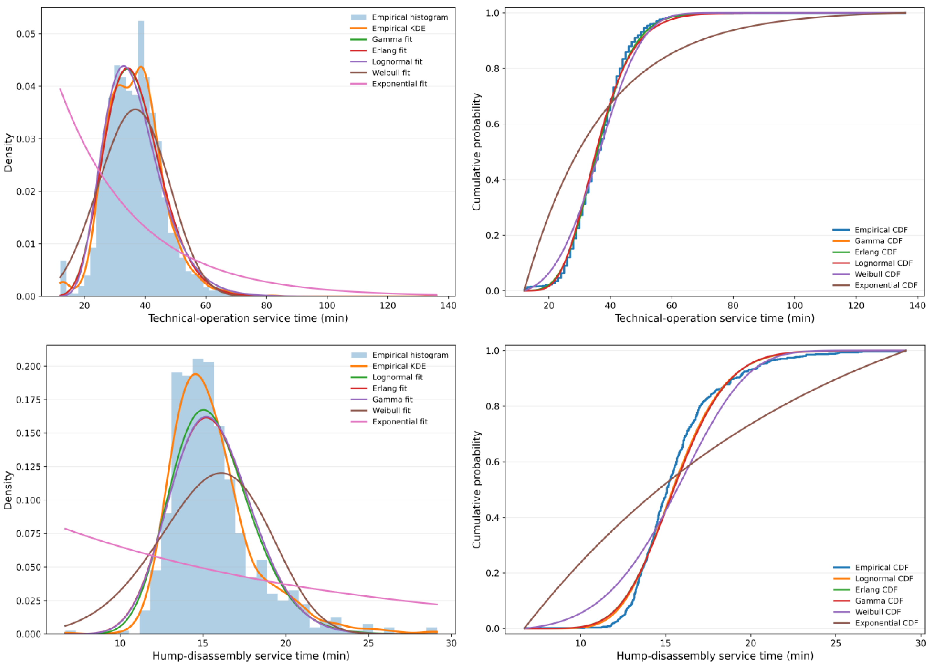
In the stochastic-service scenario, empirical distribution analysis and parametric fitting are conducted for the technical-operation and hump-disassembly service times. The PDF and CDF comparisons are shown in Figure 8. Both samples exhibit positive and right-skewed distributions. The technical-operation service time shows a wider dispersion range and a longer right tail, while the hump-disassembly service time is more concentrated around its peak interval. The Gamma/Erlang and Lognormal distributions capture the main distributional characteristics more effectively. Overall, the Gamma/Erlang family shows better agreement with the technical-operation service-time distribution, whereas the Lognormal distribution provides the best fit for the hump-disassembly service time, particularly in the tail region of the CDF.

The goodness of fit is further evaluated using the Akaike information criterion (AIC) and Bayesian information criterion (BIC) [41,42]. As shown in

Table 4. Parameter estimates and AIC/BIC comparison.

Process	Model	Parameter 1	Parameter 2	AIC	BIC
Technical operation	Gamma	shape $\alpha =14.864$	scale $\theta =2.460$	13,152.87	13,163.86
	Erlang	$k=15$	$\theta =2.438$	13,150.94	13,156.44
	Lognormal	mean $\mu =3.5653$	standard deviation σ = 0.2667	13,218.19	13,229.18
	Weibull	shape $A=40.0622$	scale $B=3.6778$	13,436.99	13,447.99
	Exponential	-	$\theta =25.546$	15,135.70	15,141.20
Hump disassembly	Lognormal	mean $\mu =2.7348$	standard deviation $\sigma =0.1567$	2874.96	2883.83
	Erlang	$k=$39	$\theta =0.400$	2898.65	2903.08
	Gamma	shape $\alpha =39.401$	scale $\theta =0.396$	2900.61	2909.48
	Weibull	shape $A=16.7436$	scale $B=5.3252$	3130.72	3139.59
	Exponential	-	$\theta =17.727$	3803.89	3808.32

, the technical-operation service time is better described by the Gamma/Erlang distribution family than by other distributions. Although the Erlang distribution gives slightly lower AIC and BIC values, it is a special case of the Gamma distribution with an integer-valued shape parameter. Considering their nearly identical fitting performance and the greater flexibility of the continuous-shape parameter, the Gamma distribution is adopted for technical-operation service-time sampling. For the hump-disassembly service time, the Lognormal distribution gives the lowest AIC and BIC values among all candidate distributions, indicating the best overall fit.

This stage-specific distribution selection is also consistent with the operational characteristics of the two service processes. Technical operations usually consist of several relatively standardized inspection and preparation activities, and their total duration tends to exhibit a moderately right-skewed distribution with relatively limited tail fluctuation; therefore, the Gamma distribution provides a suitable representation.

In contrast, hump-disassembly duration may vary with operational complexity, including train composition, the number of waggons, and the number of shunting movements, which may contribute to its right-skewed distribution and variability. Accordingly, technical-operation times are sampled from a truncated Gamma distribution over [12.00, 136.00] min, while hump-disassembly times are sampled from a truncated Lognormal distribution over [6.69, 29.13] min. This treatment avoids unrealistic negative service times and excessively extreme long-tail samples, provides a more robust statistical basis for the subsequent Monte Carlo simulation, and maintains the modelling consistency of treating each train as an indivisible service unit. Although these internal train attributes are not explicitly modelled as covariates, their aggregate effects are statistically embedded in the observed train-level hump-disassembly service-time distribution.

4.2. Baseline Simulation Analysis

Before the periodic boundary steady-state validation, a zero-initial single-day baseline simulation is conducted to compare the STEP and circular KDE arrival representations under the basic equipment-capacity configuration. All simulation experiments are implemented in MATLAB R2024a (MathWorks, Natick, MA, USA), and the DGDES procedure is used to evaluate the corresponding daily operating indicators.

To improve the empirical credibility of the model, the baseline simulation results are compared with the available field-observed indicators. The field data provide daily average values for the main observable operating indicators, including arrival volume, completed disassemblies, ${\overline{Q}}_{arr}$, $W_{qD}$, and $W_{sys}$.

Since $R_{out}$ was not included in the unified field statistical records of yard operations, a track–time load ratio is introduced as a supplementary saturation indicator to help verify the reasonableness of the simulated Rout. For operating day $d$, the track–time load ratio is defined as

$${\rho }_Y\left(d\right)=N_{arr}\left(d\right)\cdot W_{sys}\left(d\right)/C_Y\times 24\times 60$$

(20)

This indicator is not equivalent to the directly observed outside holding rate, but it provides supplementary evidence for evaluating the saturation level of the arrival–operation system.

As shown in

Table 5. Baseline simulation, field comparison, and Δt sensitivity results.

Arrival Input	$∆\mathit{t}$	Range of $\mathit{\lambda }\left(\mathit{t}\right)\mathsf{\Delta }\mathit{t}$	${\overline{\mathit{Q}}}_{\mathit{a}\mathit{r}\mathit{r}}$	${\mathit{W}}_{\mathit{q}\mathit{D}}$	${\mathit{W}}_{\mathit{q}\mathit{T}}$	${\mathit{W}}_{\mathit{s}\mathit{y}\mathit{s}}$	${\mathit{\rho }}_{\mathit{Y}}$/${\mathit{R}}_{\mathit{o}\mathit{u}\mathit{t}}$
January observed mean	1 min	—	7	74.84	2	132.8	58.76%
March observed mean	1 min	—	5.42	49.10	1.35	106.56	45.68%
January STEP	hourly	—	3.487	12.21	1.73	72.77	0
March STEP	hourly	—	3.215	8.51	1.71	68.07	0
January circular KDE	30 s	0.0095–0.0467	3.463	12.36	0.687	72.27	0
	1 min	0.0190–0.0933	3.458	12.27	1.095	72.93	0
	5 min	0.0953–0.4664	3.489	13.06	1.068	72.81	0
	10 min	0.1907–0.9296	3.540	14.26	1.068	73.88	0
	15 min	0.2879–1.3913	3.566	15.22	0.865	75.51	0
March circular KDE	30 s	0.0117–0.0394	3.255	9.07	1.43	68.93	0
	1 min	0.0234–0.0789	3.255	9.07	1.43	68.93	0
	5 min	0.1172–0.3944	3.222	8.67	1.47	68.22	0
	10 min	0.2344–0.7888	3.283	9.81	1.54	69.53	0
	15 min	0.3516–1.1831	3.267	9.34	1.82	68.19	0

, ${\rho }_Y$ is 58.76% in January and 45.68% in March, indicating a higher operating pressure in January. Under zero initial conditions, both the STEP and circular KDE baseline simulations produce substantially lower waiting-time indicators than the field-observed values, especially for $W_{qD}$, and $W_{sys}$. The $∆t$ sensitivity results for both months remain stable from 30 s to 10 min, with $\lambda \left(t\right)\mathsf{\Delta }t<1$ and only minor changes in $Q_{arr}$, $W_{qD}$, and $W_{sys}$. When $∆t$ = 15 min, $\lambda \left(t\right)\mathsf{\Delta }t$ exceeds one in both months, implying that more than one train arrival may be generated within a single time step through residual accumulation. Therefore, $∆t$ = 1 min is retained as the baseline setting for the subsequent simulations.

4.3. PSSBV Periodicity and Boundary-State Stability Analysis

In this section, the average baseline-day arrival input is repeatedly used to drive the PSSBV iteration, with the DGDES procedure serving as the day-level state-evolution kernel for computing the boundary mapping. The objective is to determine whether the boundary state remains bounded under the given arrival level, equipment capacity, and institutional service rules. This provides consistent nonzero initial boundary states for continuous-operation simulation and also evaluates whether the current arrival demand is compatible with the available processing capacity for long-term stable operation.

In the implementation, $L_{max}$ was set to 200. Because railway working diagrams are periodically adjusted, extending the search far beyond this horizon would provide limited operational meaning under an unchanged arrival-input assumption.

For the monthly baseline cases, the fitted continuous arrival intensity $\lambda \left(t\right)$ was repeatedly applied. The mean daily arrival volumes are

$${\overline{N}}_{arr}^{Jan}={\displaystyle \frac{2370}{31}}=76+{\displaystyle \frac{14}{31}}$$

(21)

$${\overline{N}}_{arr}^{Mar}={\displaystyle \frac{2297}{31}}=74+{\displaystyle \frac{3}{31}}$$

(22)

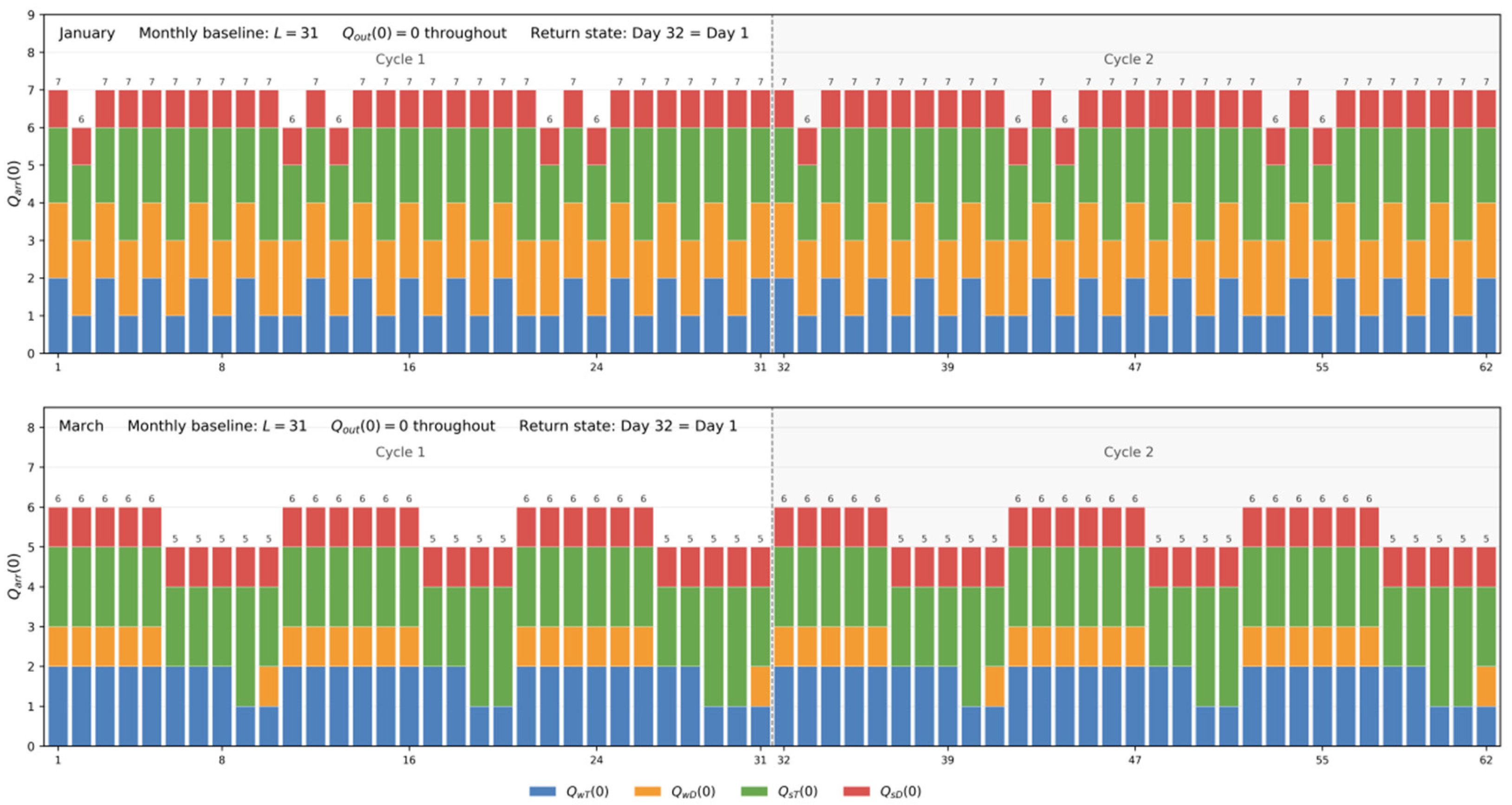
giving an arithmetic residual-phase length of $L_r=$ 31 for both months. After one complete residual-phase cycle, the boundary states remained bounded and returned to the corresponding initial phase, allowing phase-consistent nonzero boundary states to be obtained. Figure 9 shows the two-cycle evolution of periodic boundary states. For January, $Q_{arr}$ mainly fluctuates between six and seven trains, whereas for March it mainly varies between five and six trains. In both months, $Q_{out}$ remains zero throughout the periodic trajectory. These results indicate that the queueing-state variation is limited and that the detected recurrence is governed mainly by the cross-day accumulation of $r_d\left(t\right)$. Consequently, $L_r=$ 31 is consistent with $L=31$ identified by PSSBV.

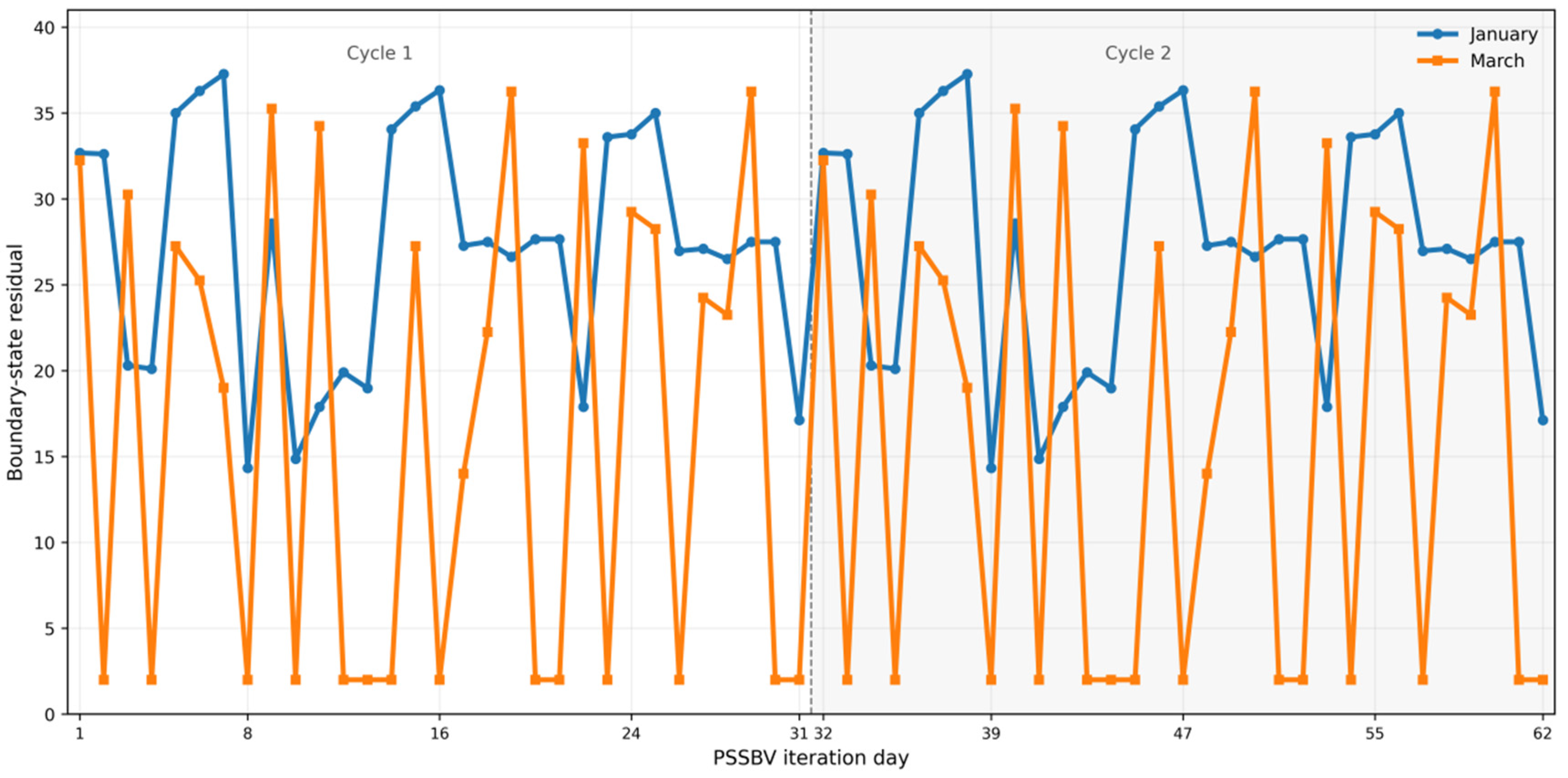
As shown in Figure 10, the boundary-state residuals for the two baseline months are evaluated after one complete arrival residual phase cycle. The results show that the residuals satisfy the prescribed convergence tolerance and that the boundary states close, ${F^{\left(L\right)}\left(x^{*}\right)=F}^{\left(Lr\right)}\left(x^{*}\right)=x^{\mathrm{*}}$.

Based on the identified periodic boundary trajectories, the 20:00 boundary states used as consistent nonzero initial conditions can be expressed as follows. For the January baseline input, $Q_{arr}=7$, $Q_{out}=0$, $Q_{wT}=2$, $Q_{wD}=2$, $Q_{sT}=2$, and $Q_{sD}=1$, the arrival residual is $r\left(0\right)=$ 14/31, the remaining processing time of the disassembly server is $I_D\left(0\right)=6.00$ min, and the remaining-processing-time vector of the four technical-operation channels is ${\mathit{I}}_{\mathit{T}}\left(0\right) = [0, 21, 6, 0]$ min. For the March baseline input, ${\mathit{Q}}_{\mathit{arr}} = 6$, ${\mathit{Q}}_{\mathit{out}} = 0$, ${\mathit{Q}}_{\mathit{wT}} = 2$, ${\mathit{Q}}_{\mathit{wD}} = 1$, ${\mathit{Q}}_{\mathit{sT}} = 2$, and ${\mathit{Q}}_{\mathit{sD}} = 1$, $\mathit{r}\left(0\right) = 3/31$ ${\mathit{I}}_{\mathit{D}}\left(0\right) = 6.25$ min, and ${\mathit{I}}_{\mathit{T}}\left(0\right) = [32.25, 0, 14.25, 0]$ min.

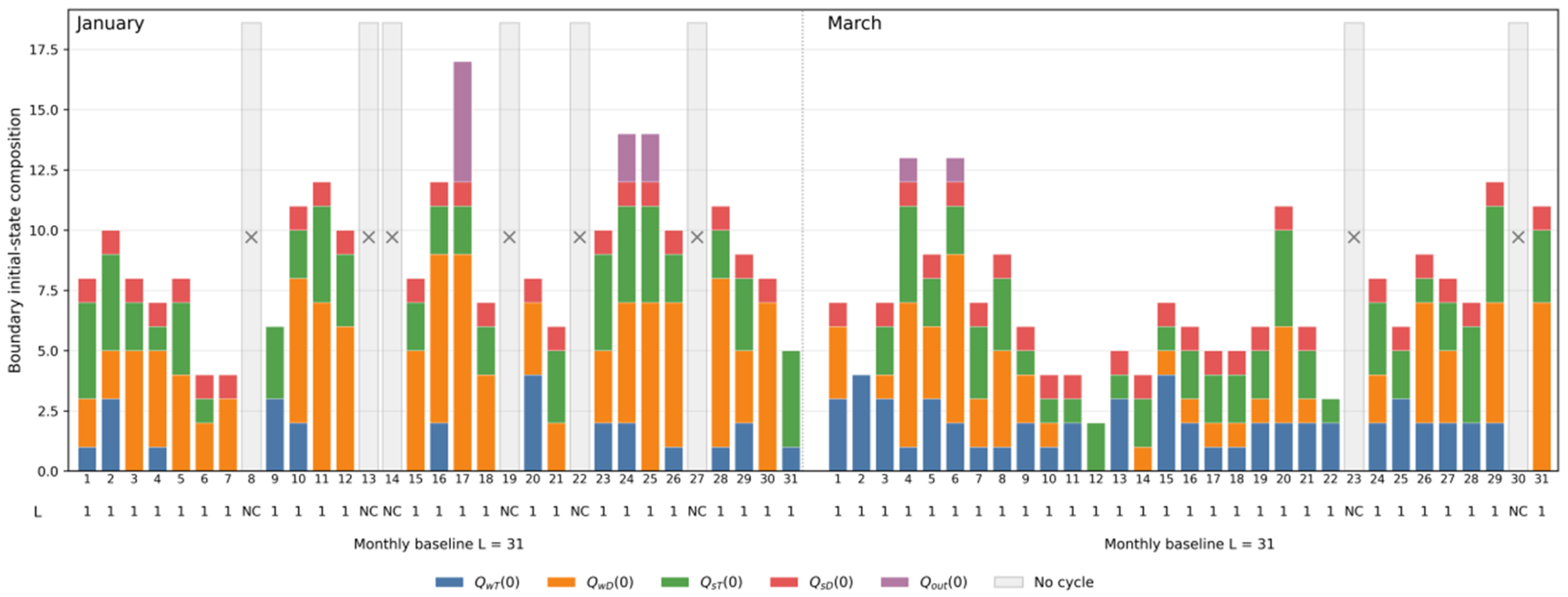
To further examine periodicity and stability under discrete arrival inputs, Figure 11 presents the daily template analysis based on the empirical train-level arrival sequences $A_d\left(t\right)$ for January and March. In this test, actual daily arrival template is repeatedly used as the input and evaluated using the PSSBV procedure. Because arrivals are triggered directly at their specified times, $r_d\left(t\right)=0$ and the arithmetic residual-phase length is $L_r=$ 1. Most templates converge to a one-day fixed boundary state with $L=1$, whereas a small number of templates are classified as NO_CYCLE.

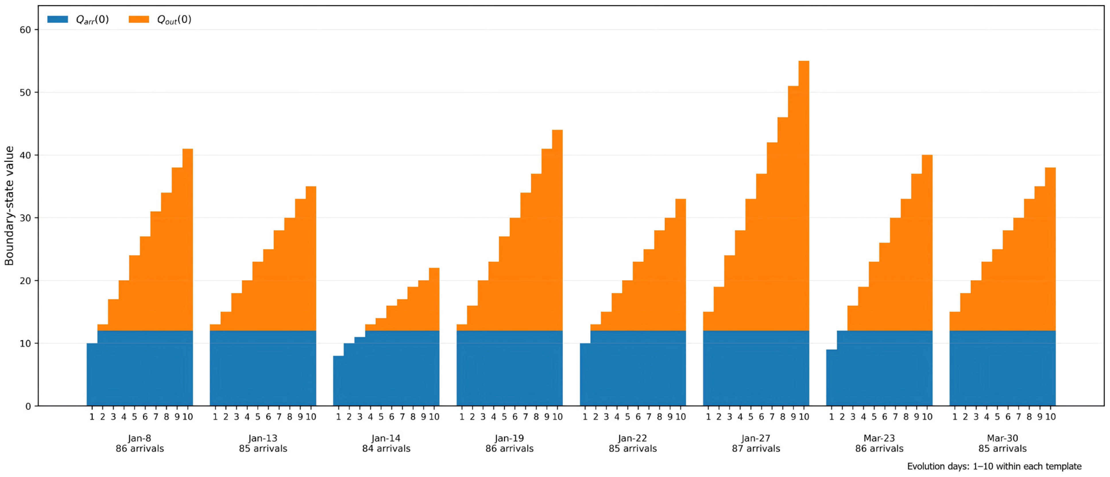
For the NO_CYCLE templates, Figure 12 further shows the boundary evolution of in-yard occupancy and outside holding during the first ten repeated evolution days. These templates generate stronger capacity pressure: $Q_{arr}\left(0\right)$ rapidly approaches the receiving-yard capacity $C_Y$, while $Q_{out}\left(0\right)$ begins to accumulate continuously. Therefore, NO_CYCLE represents an overloaded boundary evolution state rather than a closed periodic trajectory.

These results indicate that PSSBV can consistently determine the stability of both fitted continuous arrival inputs and discrete train-level sequences. Any closed periodic boundary trajectory identified by the method depends on the input structure and the corresponding operational-state configuration, rather than on an intrinsic physical cycle of the yard.

4.4. Deterministic-Service Simulation Results

This section conducts continuous-operation simulations under deterministic-service conditions using the empirical daily arrival sequence $A_d\left(t\right)$. The monthly baseline nonzero boundary state obtained from the PSSBV procedure is used as the initial condition, and the DGDES model is applied to simulate the day-to-day evolution of the arrival–operation system.

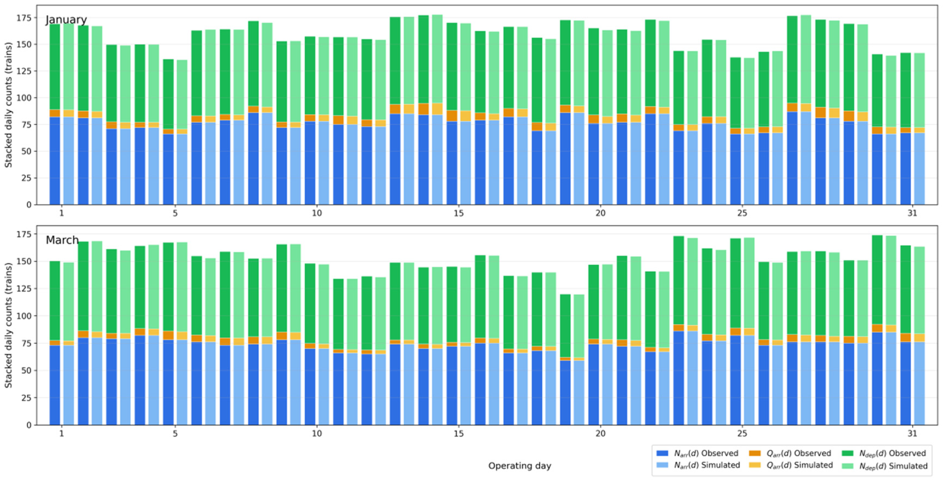
For the January and March baseline arrival–intensity inputs $\lambda \left(t\right)$, PSSBV identifies initial boundary occupancies of $Q_{arr}=7$ and $Q_{arr}=6$, respectively. Initialized with these nonzero states, the 31-day DGDESs yield mean day-start occupancies of ${\overline{Q}}_{arr}(0)=9.52$ for January and ${\overline{Q}}_{arr}(0)=7$ for March. As shown in

Table 6. Comparison of field-observed and deterministic-service simulation results.

Indicator		January Observed	Deterministic Service Times	Difference	March Observed	March Deterministic	Difference
Mean daily arrivals (trains/day)	${\overline{N}}_{arr}$	76.45	76.45	0.00	74.10	74.10	0
Mean completed disassemblies (trains/day)	${\overline{N}}_{dep}$	76.52	76.52	0.00	73.96	73.94	0.02
Mean in-yard occupancy (trains)	${\overline{Q}}_{arr}$	6.83	6.62	0.21	5.42	5.06	0.36
Mean technical waiting time (min)	${\overline{W}}_{qT}$	2.01	1.93	0.08	1.35	1.21	0.14
Mean disassembly waiting time (min)	${\overline{W}}_{qD}$	74.85	68.43	6.42	49.10	42.32	6.78
Mean system sojourn time (min)	${\overline{W}}_{sys}$	132.80	124.05	8.75	106.56	97.42	9.14
Mean outside holding rate (%)	${\overline{R}}_{out}$	--	4.52	--	--	1.89	--
Mean outside waiting time (min)	${\overline{W}}_{out}$	--	7.73	--	--	2.19	--
Mean outside holding area (train·min)	${\overline{A}}_{out}$	--	78.90	--	--	26.90	--
Mean CVIA	${\overline{CV}}_{IA}$	1.064	1.064	0	0.87	0.87	0
Mean Fano	${\overline{Fano}}_w$	0.922	0.922	0	0.64	0.64	0
Mean initial in-yard occupancy (trains)	${\overline{Q}}_{arr}\left(0\right)$	9.12	9.52	−0.40	7.40	7.00	0.4
Mean initial disassembly waiting queue (trains)	${\overline{Q}}_{wD}\left(0\right)$	5.18	5.16	0.02	2.60	2.26	0.34

, the DGDES results under deterministic-service conditions are generally consistent with the available field records for both months. The model preserves the observed daily arrival level ${\overline{N}}_{arr}$, and the simulated number of completed disassemblies ${\overline{N}}_{dep}$ is also close to the field value. For the main congestion-related indicators, the simulated mean in-yard occupancy ${\overline{Q}}_{arr}$ is close to the observed level, and the difference in technical-operation waiting time is relatively small. However, the disassembly waiting time ${\overline{W}}_{qD}$ and system sojourn time ${\overline{W}}_{sys}$ are underestimated in both January and March. Nevertheless, the DGDES can reasonably reproduce the average operating level of the system and provides a basis for analyzing congestion evolution under continuous-operation conditions.

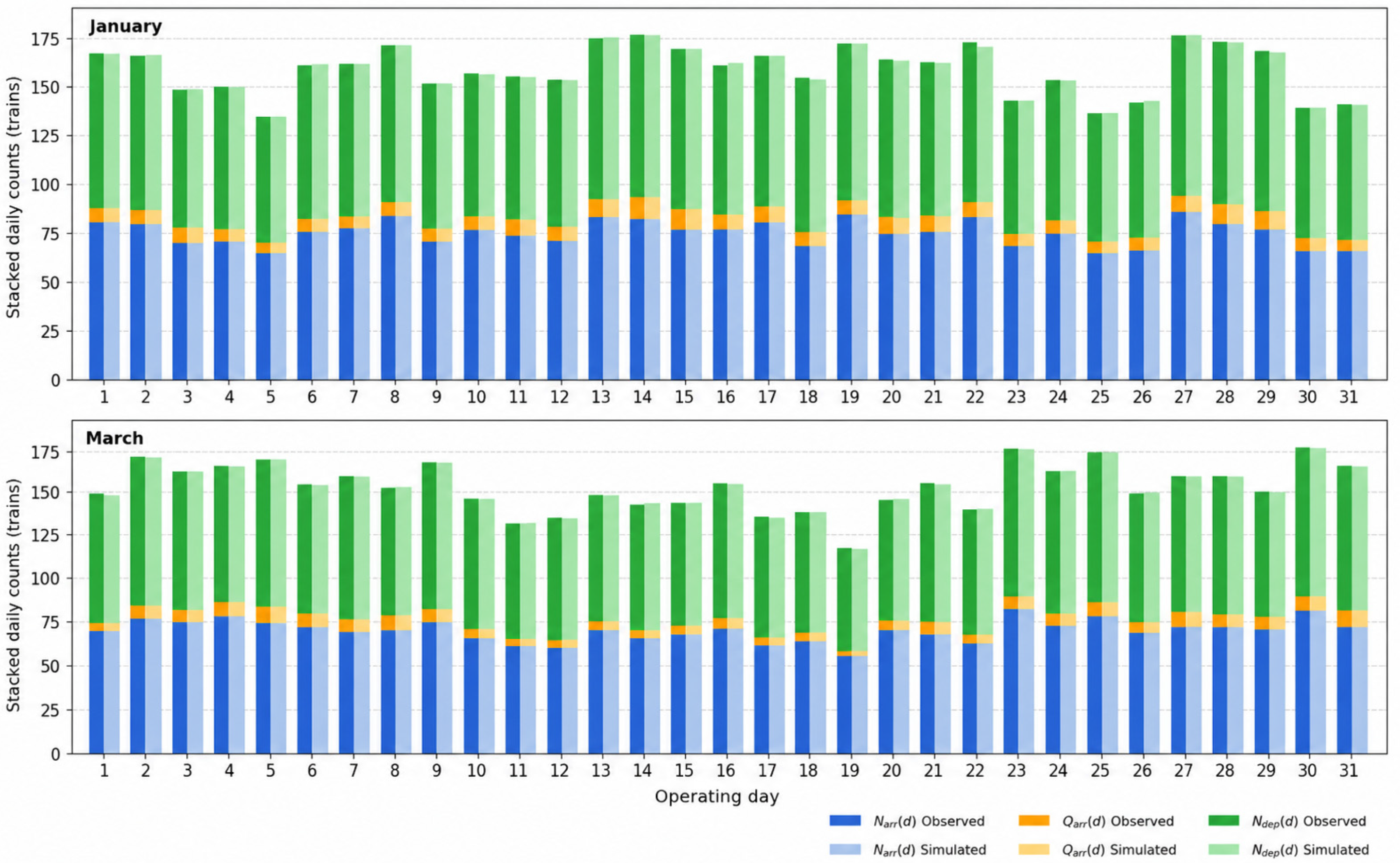
Figure 13 further compares the observed and simulated daily operating indicators. The results show that, under deterministic-service conditions, the DGDES model can reproduce the daily operating scale and the main day-to-day fluctuation patterns. The simulated daily arrivals are fully consistent with the empirical arrival input, while the completed disassemblies and mean in-yard occupancy generally follow the observed daily variations. This indicates that the DGDES model can reasonably describe the continuous day-to-day evolution of the arrival–operation system when the actual daily arrival sequence and the PSSBV-derived boundary state are used.

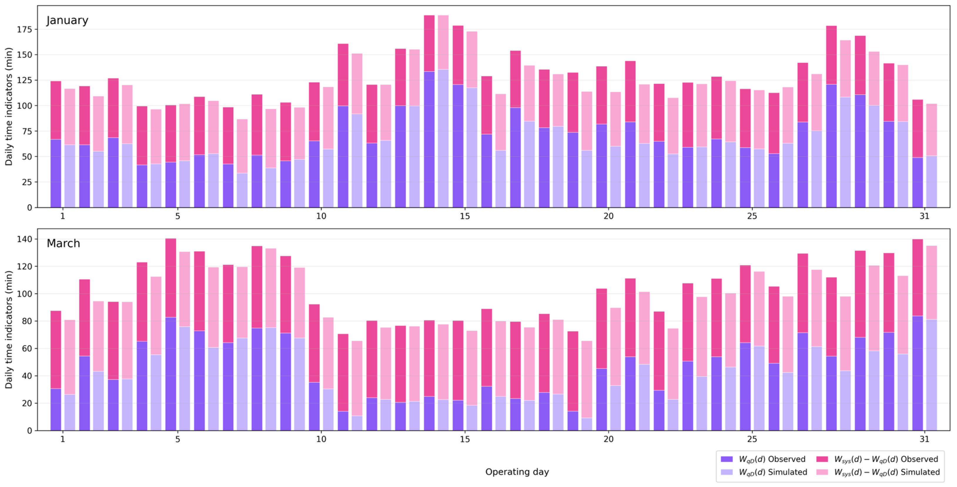
Figure 14 compares the observed and simulated daily waiting-time indicators. The DGDES model still captures the main temporal fluctuation patterns of these two indicators, especially the relative changes between low-delay and high-delay operating days. However, the simulated values of $W_{qD}\left(d\right)$ and $W_{sys}\left(d\right)$ are generally lower than the observed values in both months. This underestimation is consistent with the results in Table 6 and suggests that the deterministic-service setting, which uses mean service times, cannot reasonably reproduce the delay amplification caused by service-time variability and short-term operational disturbances in actual yard operations.

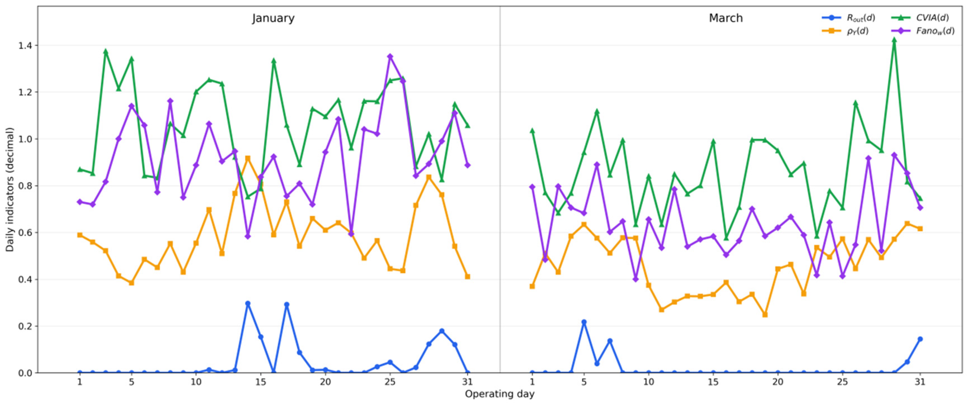
Because systematic field records of $R_{out}\left(d\right)$ are unavailable, ${\rho }_Y\left(d\right)$, ${CV}_{IA}$ and ${Fano}_w$ are used to support the interpretation of simulated outside holding risk. As shown in Figure 15, $R_{out}\left(d\right)$ and ${\rho }_Y\left(d\right)$ exhibit broadly consistent high-risk fluctuations. January shows a higher congestion level, whereas March remains relatively lower for most operating days. However, ${CV}_{IA}$ and ${Fano}_w$ do not always coincide with high outside holding risk. This indicates that, especially when the system is already operating under a high workload, arrival irregularity alone cannot fully explain the formation of outside holding risk.

To further quantify the linear and monotonic associations among candidate risk indicators, Pearson and Spearman correlation coefficients are calculated using the monthly samples [43]. As shown in

Table 7. Pearson and Spearman correlations between ${\mathrm{R}}_{\mathrm{o}\mathrm{u}\mathrm{t}}\left(\mathrm{d}\right)$ and congestion-risk indicators.

Variable	Pearson with ${\mathit{R}}_{\mathit{o}\mathit{u}\mathit{t}}\left(\mathit{d}\right)$	Spearman with ${\mathit{R}}_{\mathit{o}\mathit{u}\mathit{t}}\left(\mathit{d}\right)$	Interpretation
${\rho }_Y\left(d\right)$	0.591	0.630	positive correlation
${CV}_{IA}$	−0.106	0.004	negligible
${Fano}_w$	0.029	0.255	weak positive correlation
$Q_{arr}\left(0\right)$	0.510	0.676	positive correlation
$Q_{wD}\left(0\right)$	0.612	0.675	positive correlation
$W_{qD}\left(d\right)$	0.651	0.711	strong positive correlation
$W_{sys}\left(d\right)$	0.633	0.709	strong positive correlation
$N_{arr}\left(d\right)$	0.202	0.244	weak positive correlation

, $R_{out}\left(d\right)$ is positively correlated with ${\rho }_Y\left(d\right)$. Stronger correlations are observed for the waiting-time and residual-state indicators, especially $W_{qD}\left(d\right)$ and $W_{sys}\left(d\right)$ and $Q_{arr}\left(0\right)$. In contrast, the correlations between $R_{out}\left(d\right)$ and $N_{arr}\left(d\right)$, ${CV}_{IA}$ and ${Fano}_w$ are relatively weak.

In addition, lagged correlation coefficients are calculated to examine the cross-day propagation of congestion risk. As shown in

Table 8. Lagged correlations with current-day outside holding.

Lagged Variable	Pearson with ${\mathit{R}}_{\mathit{o}\mathit{u}\mathit{t}}\left(\mathit{d}\right)$	Spearman with ${\mathit{R}}_{\mathit{o}\mathit{u}\mathit{t}}\left(\mathit{d}\right)$	Interpretation
${\rho }_Y(d-1)$	0.539	0.572	positive correlation
${Fano}_w(d-1)$	0.170	0.326	weak positive correlation
$Q_{arr}(d-1)$	0.353	0.500	positive correlation
$Q_{wD}(d-1)$	0.383	0.452	positive correlation
$W_{qD}(d-1)$	0.490	0.569	positive correlation
$W_{sys}(d-1)$	0.482	0.586	positive correlation
$N_{arr}(d-1)$	0.422	0.390	weak positive correlation
$R_{out}(d-1)$	0.288	0.505	positive lag correlation

, the previous-day saturation level ${\rho }_Y(d-1)$, $W_{qD}(d-1)$, $W_{sys}(d-1)$, and $Q_{wD}(d-1)$ are all positively correlated with the current-day outside holding rate $R_{out}\left(d\right)$.

Based on the above results,

Table 9. Percentile-based case-specific diagnostic intervals for congestion-risk indicators.

Indicator Group		Reference Range ${<\mathit{P}}_{75}$	Warning Range $[{\mathit{P}}_{75},{\mathit{P}}_{90})$	High-Risk Tail ${\ge \mathit{P}}_{90}$	Role in Stochastic-Risk Diagnosis
Direct congestion output	$R_{out}\left(d\right)$	$<$0.013	[0.013, 0.136)	$\ge$0.136	Primary DGDES-based outside-holding risk indicator
Field-derived saturation proxy	${\rho }_Y\left(d\right)$	$<$0.590	[0.590, 0.714)	$\ge$0.714	Field-consistency indicator reflecting yard operating pressure
Daily occupancy state	${\overline{Q}}_{arr}^{\left(d\right)}$	$<$7.03	[7.03, 7.97)	$\ge$7.97	Daily in-yard occupancy pressure
Boundary residual state	$Q_{arr}\left(0\right)$	$<$10.22	[10.22, 11.00)	$\ge$11.00	Cross-day in-yard residual indicator
Boundary residual state	$Q_{wD}\left(0\right)$	$<$6.13	[6.13, 7.71)	$\ge$7.71	Pre-disassembly residual and bottleneck-pressure indicator
Waiting-time consequence	$W_{qD}\left(d\right)$	$<$73.39	[73.39, 96.68)	$\ge$96.68	Disassembly bottleneck congestion consequence
Waiting-time consequence	$W_{sys}\left(d\right)$	$<$132.34	[132.34, 153.04)	$\ge$153.04	Overall system-delay consequence
Lagged propagation	${\rho }_Y(d-1)$	$<$0.589	[0.589, 0.717)	$\ge$0.717	Previous-day saturation propagation indicator
Lagged propagation	$W_{qD}(d-1)$	$<$73.02	[73.02, 98.19)	$\ge$98.19	Previous-day disassembly delay propagation indicator
Lagged propagation	$W_{sys}(d-1)$	$<$131.82	[131.82, 154.24)	$\ge$154.24	Previous-day system-delay propagation indicator
Lagged propagation	$Q_{arr}^{(d-1)}\left(0\right)$	$<$5.66	[5.66, 7.41)	$\ge$7.41	Previous-day pre-disassembly residual propagation indicator

summarizes the case-specific diagnostic intervals for congestion-risk indicators. ${CV}_{IA}$ and ${Fano}_w$ are retained as auxiliary indicators for monitoring arrival-pattern variability and capacity matching. However, because their direct correlations with $R_{out}\left(d\right)$ are relatively weak, they are not included in the final risk-diagnostic intervals.

Since unified operational thresholds are not available for these congestion indicators, a percentile-based diagnostic method is adopted. The 75th percentile is used as the lower bound of the warning interval because it represents the upper quartile of the sample distribution, indicating that the indicator has exceeded the level of most operating days. The 90th percentile is used as the lower bound of the high-risk tail interval because it identifies the most severe operating states in the upper 10% of the sample. For the 62 operating days considered in this study, the $P_{90}$ threshold corresponds to approximately six high-tail operating days, which helps identify severe congestion while avoiding excessive dependence on a few extreme observations. Therefore, the $P_{75}$ and $P_{90}$ thresholds provide a practical balance between early warning and high-risk identification.

It should be noted that the intervals in Table 9 are case-specific and are determined by the yard layout, equipment capacity, operating rules, and empirical samples used in this study. When the proposed framework is applied to other marshalling yards, timetable periods, capacity configurations, or operating rules, the diagnostic intervals should be recalibrated using local DGDES outputs and field data.

4.5. Stochastic-Service Monte Carlo Analysis and Tail-Risk Assessment

To evaluate the effect of service-time randomness on congestion evolution and tail-risk exposure, this section uses a DGDES model with stochastic technical-operation and hump-disassembly service times to conduct 1000 Monte Carlo replications for the January and March empirical datasets under continuous-operation conditions. Specifically, $S_T$ and $S_D$ are generated according to the following truncated distributions:

$$\begin{array}{c}{S}_T\sim Truncated-Gamma(14.864, 2.460; 12.00, 136.00),\\ S_D\sim Truncated-Gamma(2.7348, 0.1567; 6.69, 29.13).\end{array}$$

During repeated simulations, the empirical arrival sequence $A_d\left(t\right)$ and the PSSBV-derived initial boundary state of the corresponding month are kept unchanged. To ensure reproducibility, a fixed base random seed was specified, and a distinct replication-specific seed was used for each run.

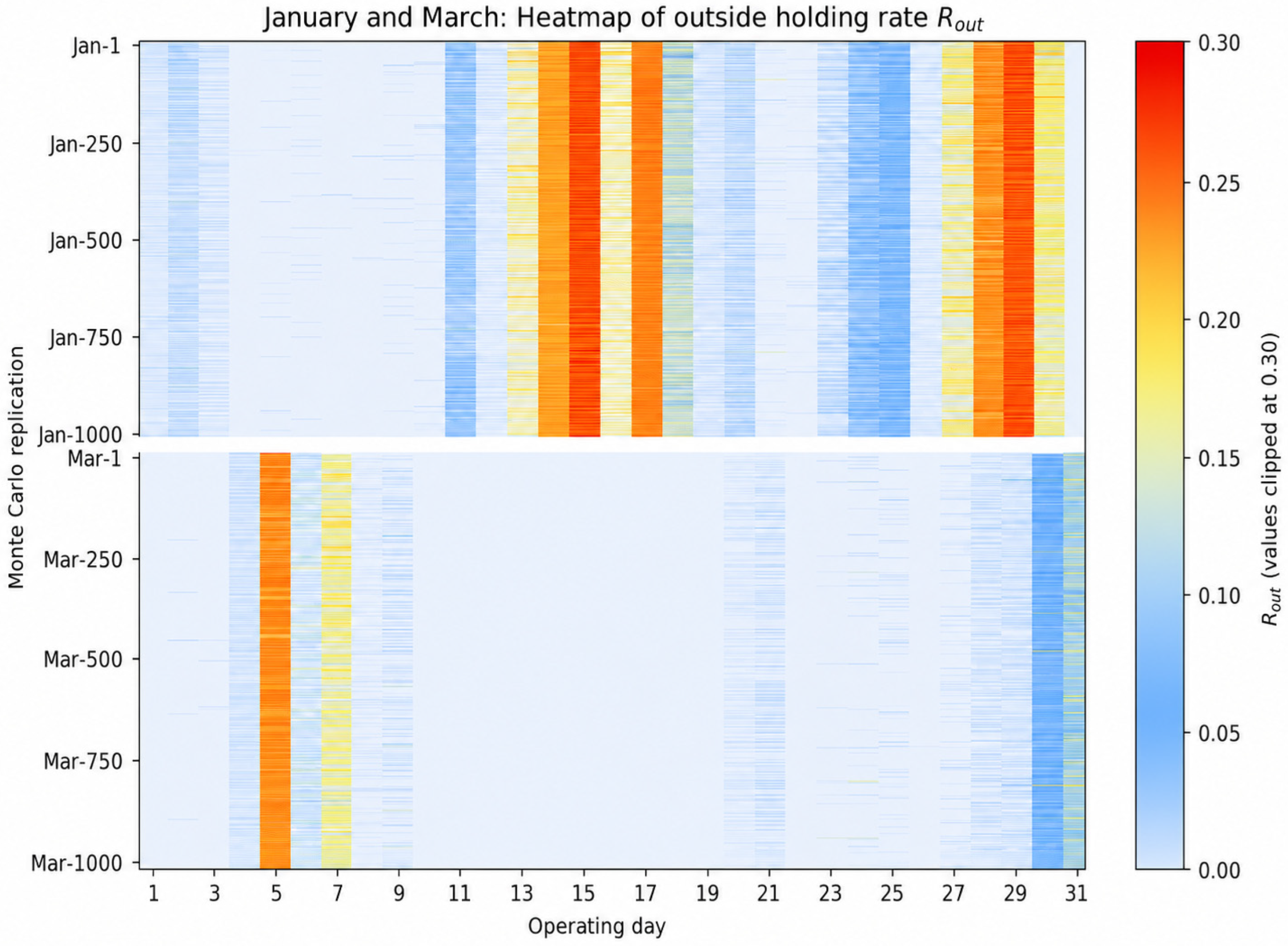
Figure 16 shows the heatmap of the outside holding rate $R_{out}\left(d\right)$ under 1000 Monte Carlo replications for January and March. The results show that high-$R_{out}\left(d\right)$ regions occur more frequently and are more concentrated in January. These operating days exhibit more evident outside holding risk. In contrast, severe outside holding patterns are much less frequent in March, indicating a more stable operating condition. Meanwhile, the high-risk regions identified under stochastic-service conditions are generally consistent with the $P_{90}$-level high-risk operating days identified under deterministic-service conditions.

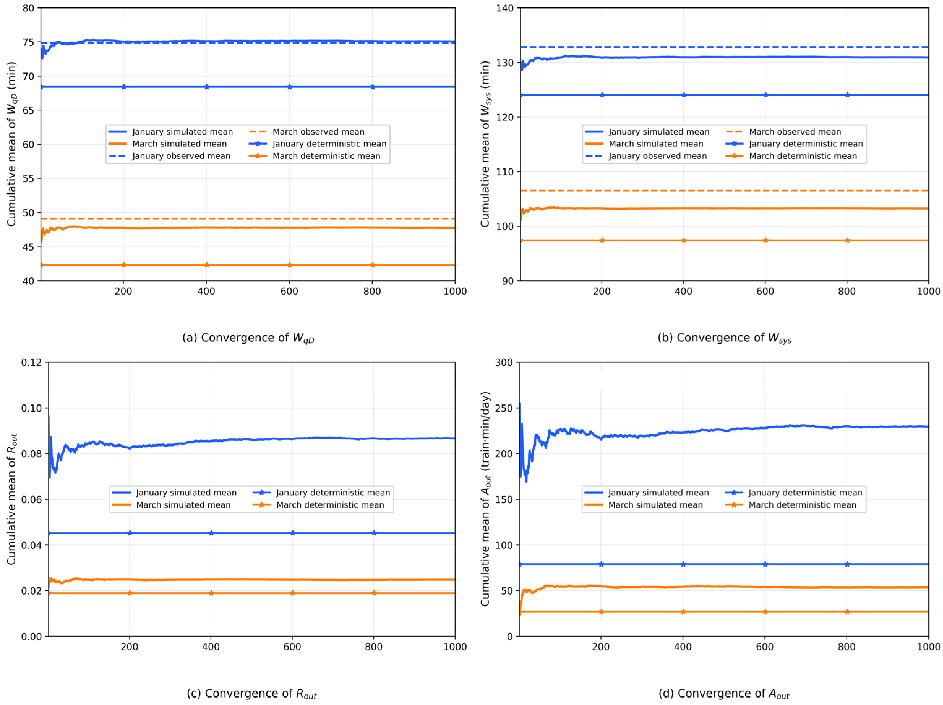
To further examine the statistical reliability of the DGDES-based stochastic simulation, the convergence behaviour of the main performance indicators is analyzed. As shown in Figure 17, the cumulative means of $W_{qD}\left(d\right)$, $W_{sys}\left(d\right)$, $R_{out}\left(d\right)$, and $A_{out}\left(d\right)$ gradually stabilize as the number of Monte Carlo replications increases. After approximately 500 replications, the variations in these indicators become limited, indicating that 1000 replications provided stable estimates for the reported indicators to obtain statistically stable stochastic-service simulation outputs.

Table 10. Comparison of field-observed and stochastic-service simulation results.

Indicator		January Observed	January Stochastic Mean	Difference	March Observed	March Stochastic Mean	Difference
Mean daily arrivals (trains/day)	${\overline{N}}_{arr}$	76.45	76.45	0	74.10	74.10	0
Mean completed disassemblies (trains/day)	${\overline{N}}_{dep}$	76.52	76.51	0.01	73.96	73.91	0.05
Mean in-yard occupancy (trains)	${\overline{Q}}_{arr}$	6.83	6.99	−0.16	5.42	5.36	0.06
Mean technical waiting time (min)	${\overline{W}}_{qT}$	2.01	2.00	0.01	1.35	1.33	0.02
Mean disassembly waiting time (min)	${\overline{W}}_{qD}$	74.85	75.07	−0.22	49.10	47.78	1.32
Mean system sojourn time (min)	${\overline{W}}_{sys}$	132.80	130.93	1.87	106.56	103.26	3.30
Mean outside holding rate (%)	${\overline{R}}_{out}$	--	8.67	--	--	2.48	--
Mean outside waiting time (min)	${\overline{W}}_{out}$	--	11.68	--	--	3.60	--
Mean outside holding area (train·min)	${\overline{A}}_{out}$	--	229.75	--	--	53.81	--
Mean CVIA	${\overline{CV}}_{IA}$	1.064	1.064	0	0.87	0.87	0
Mean Fano	${\overline{Fano}}_w$	0.922	0.922	0	0.64	0.64	0
Mean initial in-yard occupancy (trains)	${\overline{Q}}_{arr}\left(0\right)$	9.12	9.53	−0.41	7.40	7.30	0.1
Mean initial disassembly waiting queue (trains)	${\overline{Q}}_{wD}\left(0\right)$	5.18	5.18	0	2.60	2.48	0.12

compares the field observations, deterministic-service simulation results, and stochastic-service simulation results. The results show that introducing stochastic service times improves the agreement between the simulated and observed waiting-time indicators. For both January and March datasets, the observed–simulated differences in ${\overline{W}}_{qD}$ and ${\overline{W}}_{sys}$ are reduced compared with the deterministic-service setting. The stochastic-service simulation also provides closer estimates of ${\overline{Q}}_{arr}$ and ${\overline{W}}_{qT}$.

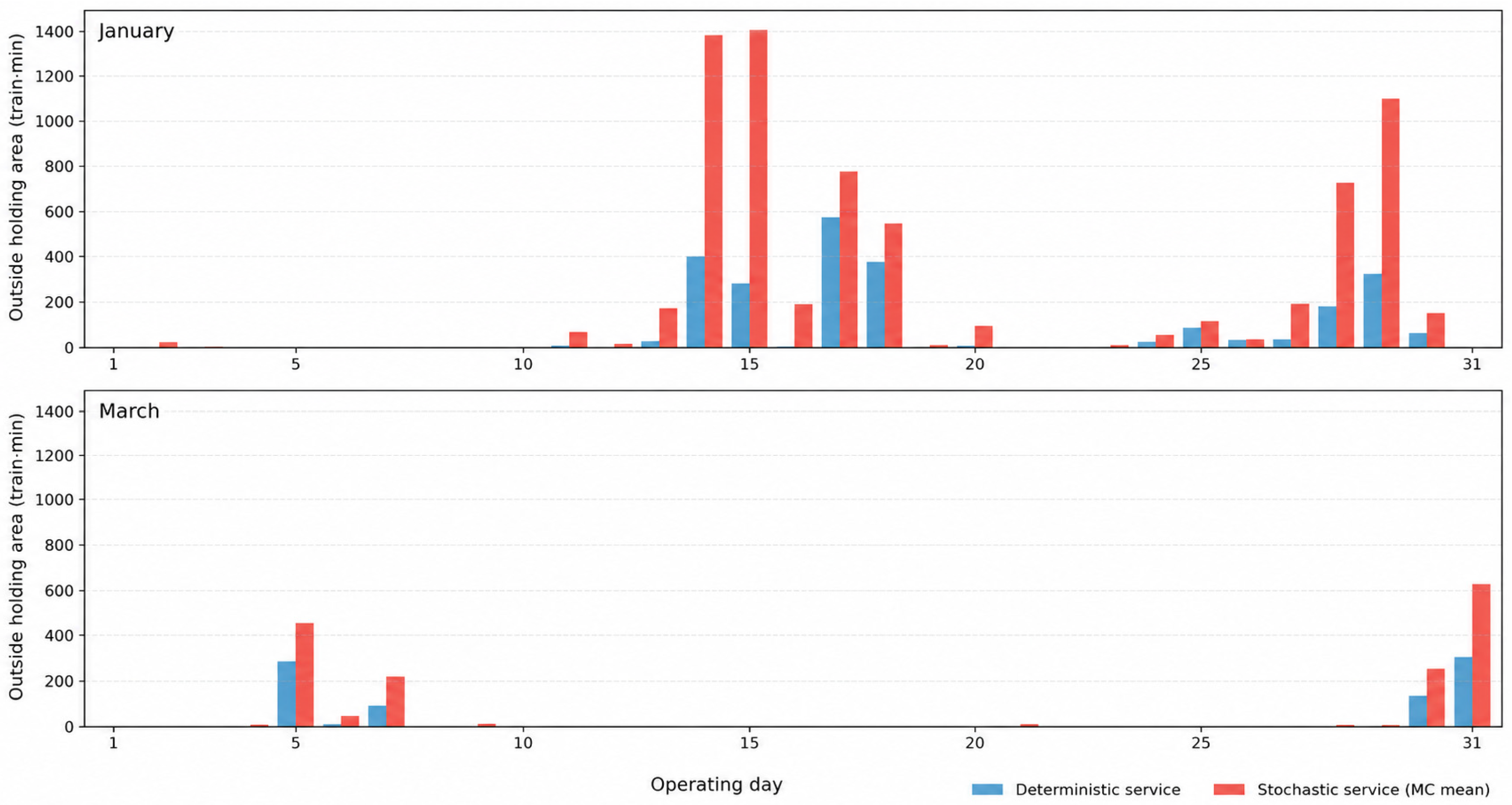
Meanwhile, the ${\overline{A}}_{out}$ increases much more than the regular waiting-time indicators after service-time randomness is introduced. To further explain this amplification effect, Figure 18 compares the $A_{out}\left(d\right)$ under deterministic and stochastic service-time settings for January and March. The results show that stochastic service times increase outside holding exposure in both months, but the amplification differs between the two datasets. The amplification of ${\overline{A}}_{out}$ in January is mainly caused by more trains being pushed into outside holding, together with longer outside waiting durations. For March, ${\overline{A}}_{out}$ increases by approximately 2.0 times, but this increase is mainly associated with longer waiting times for a limited number of outside-held trains, rather than a substantial increase in the number of trains entering outside holding.

This mechanism is more evident on high-risk operating days. For example, on Days 14 and 15 in January, both the number of outside-held trains and $W_{out}\left(d\right)$ increase markedly. As a result, $A_{out}\left(d\right)$ increases from 398 to 1394.76 train·min on Day 14 and from 281 to 1413.57 train·min on Day 15. In contrast, on Day 31 in March, the number of outside-held trains increases only slightly, from 11.00 to 12.28 trains, while $W_{out}\left(d\right)$ increases from 30.64 min to 46.83 min, causing $A_{out}\left(d\right)$ to increase from 304 to 628.40 train·min.

Figure 19 further compares the observed and stochastic-service simulated daily waiting-time indicators for the January and March datasets. The results show that the stochastic-service simulation captures the main day-to-day fluctuation patterns of both indicators. For both months, the simulated results reproduce the high-delay periods within the month. Compared with the deterministic-service results, the stochastic-service simulation is closer to the observed daily waiting-time levels and reduces the systematic underestimation of delay accumulation caused by fixed mean service times.

Based on the DGDES outputs, the percentile-based diagnostic interval method is further applied to identify the key congestion-risk indicators of the selected case, as summarized in

Table 11. Stochastic-service risk thresholds, tail-risk probabilities, and cluster-bootstrap 95% confidence intervals.

Indicator Group	Reference Range ${<\mathit{P}}_{75}$	High-Risk Tail ${\ge \mathit{P}}_{90}$	January ${\mathbf{P}(\mathit{X}\ge \mathit{P}}_{75})$	January ${\mathbf{P}(\mathit{X}\ge \mathit{P}}_{90})$	March ${\mathbf{P}(\mathit{X}\ge \mathit{P}}_{75})$	March ${\mathbf{P}(\mathit{X}\ge \mathit{P}}_{90})$
$R_{out}\left(d\right)$	$<$0.043	$\ge$0.192	34.84% [34.48, 35.18]	15.58% [15.26, 15.90]	15.19% [14.98, 15.39]	4.45% [4.27, 4.61]
${\rho }_Y\left(d\right)$	$<$0.589	$\ge$0.708	36.22% [35.89, 36.56]	18.19% [17.91, 18.46]	13.78% [13.45, 14.13]	1.81% [1.67, 1.95]
${\overline{Q}}_{arr}^{\left(d\right)}$	$<$7.11	$\ge$8.38	36.80% [36.46, 37.14]	17.36% [17.12, 17.60]	13.20% [12.92, 13.49]	2.65% [2.47, 2.82]
$Q_{arr}\left(0\right)$	$<$11.00	$\ge$12.00	42.78% [42.49, 43.07]	34.83% [34.60, 35.06]	17.25% [17.10, 17.41]	13.83% [13.67, 13.98]
$Q_{wD}\left(0\right)$	$<$6.00	$\ge$8.00	46.67% [46.34, 46.99]	23.70% [23.35, 24.05]	12.78% [12.57, 13.00]	5.39% [5.25, 5.54]
$W_{qD}\left(d\right)$	$<$76.41	$\ge$97.44	37.61% [37.27, 37.95]	17.88% [17.58, 18.16]	12.40% [12.09, 12.71]	2.12% [1.97, 2.28]
$W_{sys}\left(d\right)$	$<$132.61	$\ge$153.49	37.86% [37.51, 38.23]	18.01% [17.72, 18.30]	12.14% [11.82, 12.46]	1.99% [1.85, 2.15]
${\rho }_Y(d-1)$	$<$0.587	$\ge$0.711	38.04% [37.69, 38.40]	18.45% [18.17, 18.73]	11.96% [11.63, 12.30]	1.55% [1.43, 1.69]
$W_{qD}(d-1)$	$<$75.72	$\ge$97.47	39.65% [39.29, 40.01]	18.46% [18.15, 18.76]	10.36% [10.05, 10.68]	1.54% [1.41, 1.68]
$W_{sys}(d-1)$	$<$132.09	$\ge$153.61	39.83% [39.46, 40.21]	18.51% [18.21, 18.81]	10.18% [9.85, 10.52]	1.49% [1.37, 1.63]
$Q_{arr}^{(d-1)}(0)$	$<$6.00	$\ge$8.00	45.00% [44.66, 45.33]	22.84% [22.50, 23.18]	9.87% [9.65, 10.10]	2.48% [2.35, 2.62]

. After service-time randomness is introduced, the percentile thresholds of several core indicators show only limited changes compared with those in Table 9. In particular, the field-derived saturation ${\rho }_Y\left(d\right)$, the disassembly waiting time $W_{qD}\left(d\right)$, and the system sojourn time $W_{sys}\left(d\right)$ remain close to the original diagnostic intervals. This indicates that high waiting times and severe system delays are mainly governed by the arrival structure and the capacity constraints of the arrival–technical-operation–hump-disassembly operation chain, rather than by random service-time fluctuations alone.

To quantify the uncertainty of the estimated tail-risk probabilities, a trajectory-level cluster bootstrap was adopted [44]. For each indicator and threshold, the threshold-crossing proportion was first calculated over the complete 31-day trajectory within each replication and then averaged across the 1000 independent replications. In each bootstrap sample, complete 31-day simulation trajectories, rather than individual daily outcomes, were resampled as clusters. This treatment is consistent with the experimental structure because the system state is continuously transferred across operating days within each replication, resulting in serial dependence among daily outcomes, while all replications retain the same ordered empirical arrival sequence. The resulting 95% intervals therefore account for within-replication dependence and quantify uncertainty conditional on the fixed month-specific arrival sequence. Accordingly, the stochastic-service risk analysis provides not only diagnostic intervals based on the $P_{75}$/$P_{90}$ percentile thresholds, but also the occurrence probabilities and dependence-adjusted uncertainty intervals of different risk states. These results provide a quantitative basis for comparing congestion-risk exposure under different arrival conditions and identifying high-risk operating states.

5. Conclusions and Discussion

This study developed a hybrid fluid–queueing model and simulation-based analytical framework for analyzing congestion evolution in marshalling yard arrival operations under irregular train arrivals. The arrival–technical-operation–hump-disassembly process was modelled as a finite-capacity, multi-stage queueing system with time-varying service capacity, outside holding, gated whole-train operations, and boundary-state carryover. By integrating macroscopic mechanism analysis with train-level discrete-event simulation, the framework enables continuous-operation evaluation under practical resource and operational constraints.

Methodologically, the framework integrates two application-specific components based on established periodic-state and discrete-event simulation principles. PSSBV evaluates boundary-state stability and derives operationally reasonable initial conditions for continuous-operation simulation. DGDES then represents one-day state evolution through train admission, parallel technical operations, hump disassembly, institutional service-interruption windows, and FIFO outside holding. Their integration with the fluid–queueing representation connects congestion-mechanism analysis, boundary-state validation, and train-level performance evaluation within a computationally efficient framework. The model can also accommodate different railway operating modes by changing the arrival input. Empirical STEP, circular KDE, or observed train-level sequences can be used for dispatching-driven systems, while scheduled arrival times can be converted into deterministic periodic sequences for timetable-driven systems.

The results show that congestion is not determined solely by daily arrival volume or arrival irregularity. Although the system can maintain an approximate daily input–output balance, severe congestion emerges when concentrated arrivals interact with high residual occupancy, pre-disassembly backlog, and insufficient hump-disassembly clearance capacity. The main evolution mechanism can be summarized as follows: accumulated workload and arrival disturbances increase disassembly waiting, which raises in-yard occupancy and eventually causes congestion to spill over into outside holding.

The simulated outside holding rate $R_{out}\left(d\right)$ shows fluctuations consistent with the field-based track–time load ratio ${\rho }_Y\left(d\right)$, indicating that it serves as a useful simulation-based indicator of operational pressure. It is more strongly associated with $W_{qD}$, $W_{sys}$, and $Q_{wD}$ than with total arrivals or arrival-irregularity indicators. The lagged results further suggest that high saturation and residual workload on the preceding day can increase the likelihood of outside holding on the following day.

For diagnostic classification, these intervals should be interpreted jointly rather than independently. A high $R_{out}\left(d\right)$ with normal residual-state indicators may reflect same-day arrival concentration or temporary capacity mismatch, whereas high residual or waiting-time indicators with a low $R_{out}\left(d\right)$ may indicate internal congestion that has not yet spilled outside the yard. Congestion identification becomes more reliable when several residual-state, waiting-time, and lagged indicators enter warning or high-risk intervals simultaneously. $\mathit{C}{\mathit{V}}_{\mathit{IA}}$ and the $\mathrm{Fan}{\mathrm{o}}_{\mathrm{w}}$ factor remain useful for describing arrival variability, but their direct risk-discrimination ability weakens under high-load conditions.

After train-level service-time variability was introduced, the stochastic-service simulations reproduced the temporal evolution of congestion more closely while preserving the main locations of high-risk operating days. Service-time randomness therefore did not materially change the structural congestion pattern in the present case, but it increases the variability of waiting times and outside holding and makes tail-risk exposure more pronounced. The proposed threshold–probability diagnostic framework is consequently more suitable for operational risk identification than a single fixed threshold and can support rapid identification of high-risk operating days and proactive dispatching decisions under uncertain service conditions.

These findings have direct implications for congestion control. During low-risk periods, dispatching should focus on balancing the arrival rhythm and improving resource utilization. During warning and high-risk periods, priority should be given to reducing pre-disassembly backlog, maintaining the continuity of hump-disassembly operations, and coordinating yard admission to prevent internal congestion from spilling over into outside holding. A limitation of this study is the absence of cross-yard data comparison. Future research could incorporate data from multiple marshalling yards to compare their congestion characteristics under different operational and capacity conditions. In addition, future work could incorporate real-time operational data, rolling admission control, and dynamic disassembly–resource adjustment, and benchmark DGDES against an AnyLogic-based model to compare rapid risk assessment with detailed scenario simulation.

References

1. Iwasa, K. Rail freight in Japan—The situation today and challenges for tomorrow. Jpn. Railw. Transp. Rev. 2001, 26, 8–17. [Google Scholar]
2. European Commission, Directorate-General for Mobility and Transport. Study on Single Wagonload Traffic in Europe: Challenges, Prospects and Policy Options: Final Report; European Commission: Brussels, Belgium, 2015. [Google Scholar]
3. Dirnberger, J.R.; Barkan, C.P.L. Lean railroading for improving railroad classification terminal performance: Bottleneck management methods. Transp. Res. Rec. J. Transp. Res. Board 2007, 1995, 52–61. [Google Scholar] [CrossRef]
4. Zhao, J.; Dick, C.T. Quantifying the influence of volume variability on railway hump classification yard performance with AnyLogic simulation. Transp. Res. Rec. J. Transp. Res. Board 2023, 2677, 79–94. [Google Scholar] [CrossRef]
5. Xiao, J.; Pachl, J.; Lin, B.; Wang, J. Solving the block-to-train assignment problem using the heuristic approach based on the genetic algorithm and tabu search. Transp. Res. Part B Methodol. 2018, 108, 148–171. [Google Scholar] [CrossRef]
6. Zhang, H.; Lu, G.; Zhang, Y.; D’Ariano, A.; Wu, Y. Railcar itinerary optimization in railway marshalling yards: A graph neural network based deep reinforcement learning method. Transp. Res. Part C Emerg. Technol. 2025, 171, 104970. [Google Scholar] [CrossRef]
7. Dick, C.T. Influence of Traffic Complexity and Schedule Flexibility on Railway Classification Yard Capacity and Mainline Performance. Doctoral Dissertation, University of Illinois at Urbana, Champaign, IL, USA, 2019. Available online: https://hdl.handle.net/2142/105024 (accessed on 10 December 2025).
8. Preis, H.; Pollehn, T.; Ruf, M. Optimal resource rescheduling in classification yards considering flexible skill patterns. J. Rail Transp. Plan. Manag. 2023, 26, 100390. [Google Scholar] [CrossRef]
9. Deleplanque, S.; Hosteins, P.; Pellegrini, P.; Rodriguez, J. Train management in freight shunting yards: Formalisation and literature review. IET Intell. Transp. Syst. 2022, 16, 1286–1305. [Google Scholar] [CrossRef]
10. Boysen, N.; Fliedner, M.; Jaehn, F.; Pesch, E. Shunting yard operations: Theoretical aspects and applications. Eur. J. Oper. Res. 2012, 220, 1–14. [Google Scholar] [CrossRef]
11. Khadilkar, H.; Sinha, S.K. Rule-based discrete event simulation for optimising railway hump yard operations. In Proceedings of the 2016 IEEE International Conference on Industrial Engineering and Engineering Management (IEEM), Bali, Indonesia, 4–7 December 2016; pp. 1151–1155. [Google Scholar] [CrossRef]
12. Raut, S.; Sinha, S.K.; Khadilkar, H.; Salsingikar, S. A rolling horizon optimisation model for consolidated hump yard operational planning. J. Rail Transp. Plan. Manag. 2019, 9, 3–21. [Google Scholar] [CrossRef]
13. Vitković, N.; Marinković, D.; Stan, S.-D.; Simonović, M.; Miltenović, A.; Tomić, M.; Barać, M. Decision support system for managing marshalling yard deviations. Acta Polytech. Hung. 2024, 21, 121–134. [Google Scholar] [CrossRef]
14. Dick, C.T. Influence of mainline schedule flexibility and volume variability on railway classification yard performance. J. Rail Transp. Plan. Manag. 2021, 20, 100269. [Google Scholar] [CrossRef]
15. Zhao, J.; Dick, C.T. Quantifying the impact of classification track length constraints on railway gravity hump marshalling yard performance with AnyLogic simulation. Int. J. Comput. Methods Exp. Meas. 2022, 10, 345–358. [Google Scholar] [CrossRef]
16. Minbashi, N.; Sipilä, H.; Palmqvist, C.-W.; Bohlin, M.; Kordnejad, B. Machine learning-assisted macro simulation for yard arrival prediction. J. Rail Transp. Plan. Manag. 2023, 25, 100368. [Google Scholar] [CrossRef]
17. Minbashi, N.; Zhao, J.; Dick, C.T.; Bohlin, M. Enhancing freight train delay prediction with simulation-assisted machine learning. IET Intell. Transp. Syst. 2024, 18, 2359–2374. [Google Scholar] [CrossRef]
18. Soza-Parra, J.; Raveau, S.; Muñoz, J.C. Public transport reliability across preferences, modes, and space. Transportation 2022, 49, 621–640. [Google Scholar] [CrossRef]
19. Tirachini, A.; Godachevich, J.; Cats, O.; Muñoz, J.C.; Soza-Parra, J. Headway variability in public transport: A review of metrics, determinants, effects for quality of service and control strategies. Transp. Rev. 2022, 42, 337–361. [Google Scholar] [CrossRef]
20. Turnquist, M.A.; Blume, S.W. Evaluating potential effectiveness of headway control strategies for transit systems. Transp. Res. Rec. 1980, 746, 25–29. [Google Scholar]
21. Cox, D.R.; Lewis, P.A.W. The Statistical Analysis of Series of Events; Methuen: London, UK, 1966. [Google Scholar]
22. Rajdl, K.; Lansky, P.; Kostal, L. Fano Factor: A Potentially Useful Information. Front. Comput. Neurosci. 2020, 14, 569049. [Google Scholar] [CrossRef] [PubMed]
23. Luttinen, R.T. Statistical properties of vehicle time headways. Transp. Res. Rec. J. Transp. Res. Board 1992, 1365, 92–98. [Google Scholar]
24. Gartner, N.H.; Messer, C.J.; Rathi, A.K. (Eds.) Traffic Flow Theory: A State-of-the-Art Report; Federal Highway Administration: Washington, DC, USA, 2001.
25. Whitt, W. Fluid models for multiserver queues with abandonments. Oper. Res. 2006, 54, 37–54. [Google Scholar] [CrossRef]
26. Liu, Y.; Whitt, W. A network of time-varying many-server fluid queues with customer abandonment. Oper. Res. 2011, 59, 835–846. [Google Scholar] [CrossRef][Green Version]
27. Puha, A.L.; Ward, A.R. Fluid limits for multiclass many-server queues with general reneging distributions and head-of-the-line scheduling. Math. Oper. Res. 2022, 47, 1192–1228. [Google Scholar] [CrossRef]
28. Stolletz, R. Approximation of the non-stationary M(t)/M(t)/c(t)-queue using stationary queueing models: The stationary backlog-carryover approach. Eur. J. Oper. Res. 2008, 190, 478–493. [Google Scholar] [CrossRef]
29. Wang, W.-P.; Tipper, D.; Banerjee, S. A simple approximation for modeling nonstationary queues. In Proceedings of the IEEE INFOCOM ’96, San Francisco, CA, USA, 24–28 March 1996; pp. 255–262. [Google Scholar] [CrossRef]
30. Green, L.V.; Kolesar, P.J.; Whitt, W. Coping with time-varying demand when setting staffing requirements for a service system. Prod. Oper. Manag. 2007, 16, 13–39. [Google Scholar] [CrossRef]
31. Bogachev, M.I.; Kuzmenko, A.V.; Markelov, O.A.; Pyko, S.A. Approximate waiting times for queuing systems with variable long-term correlated arrival rates. Phys. A Stat. Mech. Its Appl. 2023, 614, 128513. [Google Scholar] [CrossRef]
32. Jennings, O.B.; Mandelbaum, A.; Massey, W.A.; Whitt, W. Server staffing to meet time-varying demand. Manag. Sci. 1996, 42, 1383–1394. [Google Scholar] [CrossRef]
33. Fu, M.C. Optimization for simulation: Theory vs. practice. INFORMS J. Comput. 2002, 14, 192–215. [Google Scholar] [CrossRef]
34. Osorio, C.; Bierlaire, M. A simulation-based optimization framework for urban transportation problems. Oper. Res. 2014, 61, 1333–1345. [Google Scholar] [CrossRef]
35. Banks, J.; Carson, J.S.; Nelson, B.L.; Nicol, D.M. Discrete-Event System Simulation, 5th ed.; Prentice Hall: Upper Saddle River, NJ, USA, 2010. [Google Scholar]
36. Law, A.M. Simulation Modeling and Analysis, 5th ed.; McGraw-Hill Education: New York, NY, USA, 2015. [Google Scholar]
37. Ross, S.M. Simulation, 5th ed.; Academic Press: Cambridge, MA, USA, 2013. [Google Scholar] [CrossRef]
38. Little, J.D.C. A proof for the queuing formula: L = λW. Oper. Res. 1961, 9, 383–387. [Google Scholar] [CrossRef]
39. Taylor, C.C. Automatic bandwidth selection for circular density estimation. Comput. Stat. Data Anal. 2008, 52, 3493–3500. [Google Scholar] [CrossRef]
40. Oliveira, M.; Crujeiras, R.M.; Rodríguez-Casal, A. A plug-in rule for bandwidth selection in circular density estimation. Comput. Stat. Data Anal. 2012, 56, 3898–3908. [Google Scholar] [CrossRef]
41. Akaike, H. A new look at the statistical model identification. IEEE Trans. Autom. Control 1974, 19, 716–723. [Google Scholar] [CrossRef]
42. Schwarz, G. Estimating the dimension of a model. Ann. Stat. 1978, 6, 461–464. [Google Scholar] [CrossRef]
43. Montgomery, D.C.; Runger, G.C. Applied Statistics and Probability for Engineers, 6th ed.; John Wiley & Sons: Hoboken, NJ, USA, 2014. [Google Scholar]
44. MacKinnon, J.G. Fast cluster bootstrap methods for linear regression models. Econ. Stat. 2023, 26, 52–71. [Google Scholar] [CrossRef]
Figure 1. Schematic layout of a marshalling yard.
Applsci 16 07553 g001
Figure 2. Queueing system for marshalling yard arrival operations.
Applsci 16 07553 g002
Figure 3. Layout of the case marshalling yard.
Applsci 16 07553 g003
Figure 4. Hourly arrival patterns and mean profile.
Applsci 16 07553 g004
Figure 5. Daily total arrivals for operational days.
Applsci 16 07553 g005
Figure 6. Comparison of baseline arrival intensity constructed by STEP, circular KDE and spline.
Applsci 16 07553 g006
Figure 7. LCV-based bandwidth selection for circular KDE.
Applsci 16 07553 g007
Figure 8. Empirical and fitted service-time distributions.
Applsci 16 07553 g008
Figure 9. Evolution of periodic boundary states.
Applsci 16 07553 g009
Figure 10. Boundary-state residual evolution.
Applsci 16 07553 g010
Figure 11. Daily template sensitivity analysis of PSSBV periodicity and boundary initial states.
Applsci 16 07553 g011
Figure 12. Boundary-state evolution under repeated NO_CYCLE daily templates.
Applsci 16 07553 g012
Figure 13. Daily operating indicators under deterministic-service conditions.
Applsci 16 07553 g013
Figure 14. Daily waiting-time indicators.
Applsci 16 07553 g014
Figure 15. Daily congestion-risk indicators.
Applsci 16 07553 g015
Figure 16. Heatmap of outside holding rate Rout(d) under 1000 Monte Carlo replications.
Applsci 16 07553 g016
Figure 17. Convergence analysis of key performance indicators.
Applsci 16 07553 g017
Figure 18. Comparison of daily outside holding area under deterministic and stochastic service-time.
Applsci 16 07553 g018
Figure 19. Observed and stochastic-service simulated daily waiting-time indicators.
Applsci 16 07553 g019