Subseasonal 2-m Temperature Prediction over East Asia Based on SwinUNet-AR

Abstract

This study focuses on subseasonal 2-m temperature prediction over East Asia for lead times of 1–6 weeks. Based on ERA5 reanalysis data from January 1982 to December 2024, multiple variables, including temperature, wind fields, and geopotential height, were selected as predictor fields. A SwinUNet-AR subseasonal prediction model integrating SwinUNet, AFNO, and Resize-Conv was constructed. The results indicate that the integrated architecture supports multiscale spatial representation, long-range dependency modeling, and high-resolution spatial reconstruction. Among different prediction strategies, simultaneous multi-lead prediction showed the most stable performance during Weeks 3–6. Multivariable input produced a statistically significant improvement in cumulative ACC during Weeks 3–6. The cumulative ACC increased by 0.07 compared with the scheme using only T2m as input, corresponding to an improvement of approximately 12.1%. The ablation experiments further indicate that the combined use of AFNO and Resize-Conv yields a modest improvement in medium- and extended-range forecast skill, particularly in cumulative ACC. Compared with the baseline SwinUNet, SwinUNet-AR reduced the mean RMSE by 0.02 °C during Weeks 3–4 and 0.03 °C during Weeks 5–6, while increasing the cumulative ACC during Weeks 3–6 by 0.04, corresponding to an improvement of approximately 7.4%. Compared with raw CFSv2 forecasts, SwinUNet-AR reduced the mean RMSE over Weeks 1–6 by 0.84 °C, corresponding to a reduction of approximately 44.9%. During Weeks 4–6, the mean RMSE was approximately 0.83 °C lower, corresponding to a reduction of about 40.8%. In terms of ACC, SwinUNet-AR achieved values comparable to those of CFSv2 during Weeks 4–6 and slightly higher values at some lead times. Overall, SwinUNet-AR shows potential for improving medium- and extended-range subseasonal 2-m temperature prediction over East Asia and provides a useful data-driven framework for regional subseasonal forecasting.

1. Introduction

In recent years, against the background of ongoing global warming, extreme temperature events have occurred frequently over East Asia. Regional mean temperatures have generally increased, and winter temperatures have repeatedly reached record-high levels. Meanwhile, severe cold surges still occur episodically. The coexistence of anomalous warmth and severe cold has increased temperature variability and complicated regional temperature prediction over East Asia. Pronounced temperature fluctuations on interannual and intraseasonal time scales not only increase the uncertainty of regional climate system evolution, but also pose serious challenges to power dispatching, agricultural production, transportation, and public safety. Therefore, improving temperature prediction skill over East Asia, particularly at lead times of several weeks, is important for understanding subseasonal temperature variability and could support disaster prevention, risk management, and socioeconomic planning [1,2,3].

Subseasonal prediction generally refers to forecasts on the time scale of 1–6 weeks. It lies between weather prediction and seasonal prediction and serves as an important bridge connecting weather and climate prediction [3,4,5]. Compared with weather forecasts within about two weeks, subseasonal prediction can provide a longer lead time for decision-making. Compared with monthly or seasonal climate predictions, subseasonal forecasts can describe the occurrence, development, and persistence of intraseasonal anomalies at a finer temporal resolution [6]. Subseasonal forecasts therefore have potential applications in agricultural planning, water-resource management, energy-system operation, and the assessment of persistent temperature anomalies. However, subseasonal prediction is also one of the most challenging components of current forecasting systems. Due to the strong nonlinearity and chaotic nature of the atmospheric system, the influence of initial conditions weakens markedly on the 1–6-week time scale, while slowly varying boundary forcings such as sea surface temperature, sea ice, and soil moisture have not yet fully established a dominant role. As a result, this time scale lacks both strong initial-condition constraints and stable boundary-signal support, leading to generally low forecast skill. It is therefore often referred to as the “predictability desert” [7,8]. This challenge is even more pronounced over East Asia, where the complex monsoon system interacts with mid- and high-latitude atmospheric circulation.

With the growing integration of artificial intelligence and atmospheric science, machine learning- and deep learning-based subseasonal prediction methods have become an active research topic. Compared with traditional statistical methods, artificial intelligence models can automatically extract complex nonlinear relationships and high-dimensional spatiotemporal features from large-scale historical data. Compared with dynamical prediction systems, they may also offer advantages in computational efficiency, multisource data integration, and rapid model development. Existing studies generally follow two approaches: post-processing dynamical-model outputs and developing direct data-driven subseasonal prediction models. Previous studies have shown that methods such as XGBoost, LSTM, CNN-LSTM, and U-Net can improve prediction skill to some extent in temperature and precipitation forecasting tasks. Meanwhile, the emergence of AI-based weather forecasting systems, such as Pangu-Weather, FengWu, FuXi, and GraphCast, has also accelerated advances in weather and climate prediction [9,10,11,12,13,14,15,16].

In addition to general deep learning forecasting frameworks, several network components originally developed in computer vision and scientific machine learning have shown potential for gridded geophysical prediction. SwinUNet combines the hierarchical representation capability of the Swin Transformer with a U-shaped encoder–decoder structure and has been widely used in dense prediction tasks because it can capture multiscale spatial features while maintaining computational efficiency. This structure is suitable for meteorological fields with both regional gradients and large-scale spatial organization. AFNO provides an efficient frequency-domain token-mixing mechanism and has been successfully applied in data-driven weather forecasting systems such as FourCastNet, demonstrating its ability to represent global interactions and large-scale atmospheric patterns [17]. Meanwhile, Resize-Conv has been introduced as an alternative to transposed convolution to reduce checkerboard artifacts during upsampling, which is particularly important for continuous gridded variables such as temperature fields where spatial smoothness and structural consistency need to be preserved [18]. These studies indicate that SwinUNet, AFNO, and Resize-Conv each address key challenges in gridded-field prediction, namely multiscale feature extraction, long-range dependency modeling, and high-resolution spatial reconstruction. However, their combined application to regional subseasonal 2-m temperature prediction over East Asia has not been fully explored.

AI-based subseasonal prediction is still at a relatively early stage. Existing models often show limited stability at longer lead times, difficulty in maintaining physical consistency, and limited ability to represent extreme events. Over-smoothing and amplitude attenuation are also common. Moreover, most models are designed for global forecasting or optimized primarily using domain-averaged statistical objectives and may not adequately capture the pronounced spatial heterogeneity of East Asia. In particular, current methods remain limited in representing long-range dependencies and extracting low-frequency signals during Weeks 3–6.

Although recent deep learning models have achieved substantial progress in medium-range and subseasonal weather forecasting [19,20], several gaps remain in regional subseasonal 2-m temperature prediction over East Asia. First, Swin Transformer introduced shifted-window attention for hierarchical multiscale representation, whereas SwinUNet incorporated Swin Transformer blocks into a U-shaped encoder–decoder architecture [21,22]. However, the original formulations of these architectures do not explicitly include frequency-domain modeling of large-scale, slowly varying signals relevant to East Asian subseasonal temperature predictability [23,24]. Second, AFNO provides an efficient mechanism for global token mixing in the Fourier domain [25] and has been successfully employed in FourCastNet for global high-resolution weather forecasting [17]. Nevertheless, AFNO-based architectures such as FourCastNet do not inherently include a U-shaped multiscale decoder with skip connections. Their direct application to a heterogeneous regional domain may therefore not fully balance global signal representation and the recovery of regional spatial details. Third, recent global AI forecasting systems include Pangu-Weather [9], FuXi [12], and GraphCast [16] for medium-range weather forecasting, FengWu-W2S [13] for seamless weather-to-subseasonal forecasting, and FuXi-S2S [20] for subseasonal forecasting. However, their prediction targets, spatial scales, model configurations, and verification settings differ from the regional weekly-mean subseasonal temperature prediction problem considered here. Therefore, there remains a need for a regional deep learning framework that can jointly represent multiscale spatial heterogeneity, large-scale low-frequency background signals, and smooth spatial reconstruction for East Asian subseasonal temperature prediction.

East Asia provides a particularly suitable yet challenging test region because its subseasonal temperature variability is influenced by complex interactions among the East Asian monsoon, land–sea thermal contrast, the Tibetan Plateau, midlatitude circulation anomalies, and regional topographic effects [23,24,26,27]. These factors lead to the coexistence of broad-scale coherent anomaly patterns and strong regional spatial heterogeneity. Accordingly, this study develops SwinUNet-AR as a task-oriented architecture for East Asian subseasonal 2-m temperature prediction. Compared with the standard SwinUNet architecture, the proposed model introduces AFNO at the bottleneck layer to enhance the representation of large-scale low-frequency signals and long-range spatial dependencies. In addition, Resize-Conv is adopted in the decoder to reduce checkerboard artifacts during upsampling [18] and support smoother reconstruction of continuous temperature fields. Unlike AFNO-based global architectures, SwinUNet-AR retains the hierarchical encoder–decoder structure and skip connections of SwinUNet, allowing the model to balance global signal extraction with the recovery of regional spatial details. The novelty of this study therefore lies not in proposing each module independently, but in designing and verifying a regional subseasonal forecasting framework that integrates multiscale spatial representation, frequency-domain modeling of low-frequency signals, and artifact-reduced spatial reconstruction for East Asia.

To address these issues, this study focuses on subseasonal 2-m temperature prediction over East Asia and constructs a deep learning model that integrates SwinUNet, AFNO, and Resize-Conv. The proposed model uses SwinUNet as the backbone to extract multiscale spatial features. An AFNO module is introduced into the bottleneck layer to enhance the representation of large-scale low-frequency signals and long-range dependencies. In the decoder, Resize-Conv is adopted to improve the recovery of high-resolution features, reduce upsampling artifacts, and enhance the reconstruction quality of spatial details. Based on ERA5 reanalysis data, this study constructs a multivariable sample dataset over East Asia, conducts systematic experiments on predictor selection, prediction strategies, and the contributions of key modules, and further compares the proposed model with the dynamical model CFSv2. The prediction performance of the proposed model is comprehensively evaluated at different lead times, with particular emphasis on Weeks 3–6. This study aims to develop and evaluate a deep learning framework for regional subseasonal temperature prediction over East Asia and to provide guidance for the development of regional AI-based forecasting systems.

2. Materials and Methods

2.1. Data and Preprocessing

This study used the ERA5 reanalysis dataset released by the European Centre for Medium-Range Weather Forecasts (ECMWF, Reading, UK) as the primary data source for subseasonal 2-m temperature prediction over East Asia. ERA5 integrates multisource information, including satellite observations, radiosonde observations, and surface observations, through advanced data assimilation and numerical modeling systems. It provides hourly estimates of a wide range of atmospheric, land, and oceanic variables with high spatial and temporal consistency. Previous studies have demonstrated the reliability and broad applicability of ERA5 in meteorological and climatological research, including global climate reanalysis, precipitation and climate monitoring, land-surface hydroclimate analysis, and regional weather and climate evaluation. Therefore, ERA5 was selected as the primary reference dataset for constructing predictor fields and verifying subseasonal 2-m temperature forecasts in this study [28,29,30]. The ERA5 data used in this study covered the period from January 1982 to December 2024. The original ERA5 data were 0.25° × 0.25° regridded to a regular 1.5° × 1.5° latitude–longitude grid over East Asia using bilinear interpolation, and daily mean fields were then constructed for subsequent model training and verification.

Figure 1 shows the geographical location of the study area and the model verification domain. The study area covers East Asia, including China, the Korean Peninsula, Japan, Mongolia, parts of Southeast Asia, and adjacent oceanic regions. This domain contains complex land–sea contrasts, the Tibetan Plateau, monsoon-influenced regions, and midlatitude circulation zones, which together contribute to strong spatial heterogeneity in subseasonal 2-m temperature variability. The ERA5 and CFSv2 fields used in this study were uniformly interpolated onto a regular 1.5° × 1.5° latitude–longitude grid over this domain to ensure consistent model training and verification.

To characterize the atmospheric thermal and dynamical background affecting subseasonal temperature variations over East Asia, multiple meteorological variables at the surface and at key pressure levels, including 850 hPa, 500 hPa, and 200 hPa, were selected as model input variables (

Table 1. Variable information of the reanalysis dataset.

Variables	Source	Levels	Unit	Resolution
T	ERA5	850, 500, 200 hPa	K
U	ERA5	850, 500, 200 hPa	m s−1
V	ERA5	850, 500, 200 hPa	m s−1
Z	ERA5	850, 500, 200 hPa	m2 s−1
Rh	ERA5	850, 500, 200 hPa	%	0.25 × 0.25°
T2m	ERA5	2 m	K
U10	ERA5	10 m	m s−1
V10	ERA5	10 m	m s−1
SP	ERA5	Surface	Pa

). These variables include temperature (T), zonal wind (U), meridional wind (V), geopotential height (Z), relative humidity (Rh), 2-m temperature (T2m), 10-m zonal wind (U10), 10-m meridional wind (V10), and surface pressure (SP). Among them, the 850-hPa level mainly reflects lower-tropospheric circulation and thermal transport characteristics, the 500 hPa level represents the mid-tropospheric circulation pattern, and the 200 hPa level provides important information on upper-level jets and large-scale atmospheric waves. Together, these variables form the multivariable gridded inputs used for subseasonal temperature prediction.

To improve the quality of model inputs and highlight predictable signals on the subseasonal time scale, all raw data were preprocessed in a unified manner. First, to reduce the influence of high-frequency weather-scale disturbances without introducing future information, a trailing 7-day moving average was applied to all input variables. For an initialization date (t), only data from (t − 6) to (t) were used, and no post-initialization data were included. Specifically, the daily values over seven consecutive days were averaged with equal weights, and a new time series was generated by moving the window forward day by day, as follows:

$$X_{filtered}\left(t\right)={\displaystyle \frac{1}{7}}{\displaystyle \sum _t^{t+6}} X\left(i\right)$$

(1)

To further clarify the construction of the input–target pairs, an initialization date (t) was defined for each sample. Under the default one-week historical input setting, the model input (X_t) was constructed from the 7-day mean multivariable ERA5 fields from day (t − 6) to day (t):

$$X_t={\displaystyle \frac{1}{7}}{\displaystyle \sum _{d=t-6}^t} V(d)$$

(2)

where (V(d)) denotes the daily ERA5 predictor field on day (d). The prediction target was not a daily value, but a non-overlapping weekly mean 2-m temperature field after the initialization date. For lead week (k), the target field was defined as

$$Y_t^{(k)}={\displaystyle \frac{1}{7}}{\displaystyle \sum _{d=t+7(k-1)+1}^{t+7k}} T2m(d),k=1,\dots ,6$$

(3)

Accordingly, Weeks 1 to 6 are defined as the non-overlapping 7-day means of days 1–7, 8–14, 15–21, 22–28, 29–35, and 36–42 after initialization, respectively, using forward-looking windows rather than centered averages.

On this basis, the input variables were further standardized to reduce the influence of differences in magnitude among different variables during model training. For temperature, wind, geopotential height, and surface pressure variables, Z-score standardization was applied using the mean and standard deviation calculated from the training period. Relative humidity was treated differently because it is a bounded percentage variable with a relatively stable physical range. Retaining its original percentage values helps preserve the physical meaning of humidity saturation and avoids changing the interpretation of dry and humid conditions. Since the magnitude of relative humidity is limited compared with variables such as geopotential height and surface pressure, retaining raw RH values did not introduce large-scale numerical imbalance in the input fields. In addition, the model contains normalization operations during feature extraction, which further reduces the potential influence of this scale difference on training stability. All other variables were standardized using the Z-score method:

$$X_{norm}={\displaystyle \frac{X-\mu }{\sigma }}$$

(4)

where μ denotes the sample mean and σ denotes the sample standard deviation. After the above preprocessing, the numerical scales of the different variables were made comparable, thereby improving the stability and convergence of model training.

In terms of sample construction and data splitting, the raw dataset spans from 1 January 1982 to 31 December 2024, containing a total of 15,706 daily samples. After applying the 7-day moving average, the total number of samples was reduced to 15,700. A chronological split was adopted between model development and independent testing. Data from 1982–2018 were used for model development and were randomly divided into training and validation subsets at a ratio of 9:1, whereas data from 2019–2024 were reserved as an independent chronological test set. Data from 1 January 1982 to 31 December 2018 were used as the training and validation period, containing 13,514 daily samples. After the moving-average processing, 13,508 samples were obtained and randomly divided into the training and validation sets at a ratio of 9:1, resulting in 12,157 training samples and 1351 validation samples. Data from 1 January 2019 to 31 December 2024 were selected as the test set, containing 2192 daily samples. After moving-average processing, 2186 samples were obtained. This splitting strategy ensures a sufficient number of training samples while enabling a relatively objective evaluation of the model’s generalization ability on recent independent samples. Samples whose target windows crossed the training–testing boundary were excluded to avoid information leakage between the training/validation and independent test periods. Although adjacent daily samples may share part of their input windows, this overlap only introduces temporal dependence and does not introduce future information into the predictors. The temporal split was designed to ensure chronological independence between model development and final evaluation. The period 1982–2018 was used for training and validation because it provides a long historical sample covering multiple interannual and decadal variability conditions, which is necessary for learning subseasonal temperature relationships from reanalysis data. The period 2019–2024 was reserved as an independent test period because it represents the most recent years in the dataset and was not used during model training or validation. This setting avoids information leakage from future samples into the training process and provides an out-of-sample evaluation of model generalization under recent climate conditions. The six-year test period also provides a relatively large number of daily initialization samples for evaluating weekly mean forecasts from Weeks 1 to 6.

For comparison with the proposed SwinUNet-AR model, CFSv2 2-m temperature forecasts were used as the dynamical-model benchmark. CFSv2 is a coupled dynamical prediction system developed by the National Centers for Environmental Prediction. Specifically, the dynamical benchmark was based on the NCEP CFSv2 operational real-time forecasts and historical reforecasts. The CFSv2 data used in this study include real-time forecasts for 2017–2024 and historical reforecasts for 1999–2017, with 32 ensemble members. The original CFSv2 forecasts are available at a 6-hourly temporal resolution. To obtain daily forecast fields, the four forecasts within each day were first averaged to produce daily means for each ensemble member.

To ensure a consistent verification framework with SwinUNet-AR, the CFSv2 daily forecasts were further aggregated into the same non-overlapping lead-week windows as the SwinUNet-AR targets. Specifically, Lead Week 1 was defined as forecast days 1–7, Lead Week 2 as forecast days 8–14, Lead Week 3 as forecast days 15–21, and so on until Lead Week 6, which corresponds to forecast days 36–42. The 32 ensemble members were averaged to obtain the deterministic ensemble-mean CFSv2 forecast. The CFSv2 fields were then interpolated onto the same 1.5° × 1.5° latitude–longitude grid as ERA5 using bilinear interpolation. The same East Asian verification domain and the same verification period were used for both SwinUNet-AR and CFSv2. Unless otherwise stated, the CFSv2 forecasts were evaluated as raw model outputs without additional bias correction. For the ACC comparison, CFSv2 anomalies were calculated relative to the CFSv2 lead-dependent model climatology derived from the historical reforecast period, while ERA5 anomalies were calculated relative to the ERA5 climatology over the same reference calendar periods. The real-time verification period was excluded from the climatology calculation.

2.2. SwinUNet-AR Model

For the task of subseasonal 2-m temperature prediction over East Asia, this study constructed a deep learning model named SwinUNet-AR (Figure 2), which integrates SwinUNet, AFNO, and Resize-Conv. The subseasonal time scale lies between weather processes and seasonal climate variability. The prediction target therefore includes both large-scale low-frequency anomaly signals and pronounced regional and local variations. Accordingly, the model should be capable of extracting multiscale spatial features, effectively representing long-range dependencies across regions, and maintaining the continuity and stability of spatial structures during output reconstruction. Traditional convolutional neural networks have certain limitations in terms of receptive field and global information modeling, whereas standard Transformers, despite their strong global modeling capability, are computationally expensive for high-resolution gridded-field prediction [31]. SwinUNet introduces the Swin Transformer into a U-shaped encoder–decoder framework, achieving a balance between hierarchical feature representation and computational efficiency, and thus provides a suitable backbone structure for regional meteorological gridded-field prediction. Therefore, this study adopted SwinUNet as the backbone network and made targeted modifications to its bottleneck layer and decoder for subseasonal temperature anomaly prediction, thereby forming the SwinUNet-AR model.

Rather than simply stacking AFNO onto SwinUNet, the proposed architecture places AFNO only at the bottleneck layer, where the spatial resolution is lowest and the feature representation is most suitable for extracting large-scale low-frequency signals. This design avoids excessive frequency-domain mixing at high-resolution layers while preserving the local and regional multiscale representations learned by the Swin Transformer encoder. In the decoder, Resize-Conv is introduced to improve the reconstruction of continuous gridded temperature fields and to reduce possible checkerboard artifacts caused by transposed convolution. For reproducibility, the main architectural settings of SwinUNet-AR are further specified as follows. The model uses a patch size of 4 × 4 and a patch embedding dimension of 96. The Swin Transformer encoder consists of four stages with depths of [2, 2, 2, 2], and the decoder depths are [1, 2, 2, 2]. The numbers of attention heads in the four encoder stages are [3, 6, 12, 24], and the local window size is 7 × 7. The MLP ratio is set to 4.0, QKV bias is used, patch normalization is enabled, and absolute position embedding is not used. The dropout, attention-dropout, and stochastic-depth rates were all set to 0.1. The AFNO module is inserted only at the bottleneck layer, with one lightweight AFNO block consisting of LayerNorm, two-dimensional Fourier transform, real- and imaginary-part linear mixing, inverse Fourier transform, dropout, and residual connection. In the decoder, the final upsampling is performed using two consecutive Resize-Conv blocks. Each Resize-Conv block uses bilinear interpolation for 2× upsampling, followed by a 3 × 3 convolution, GroupNorm, and GELU activation. A final 1 × 1 convolution maps the reconstructed feature maps to six output channels, corresponding to weekly mean T2m forecasts for lead weeks 1–6.

In terms of the overall architecture, the model first receives historical multivariable gridded fields as input, divides them into patches, and maps them into token sequences. Then, multiscale spatial features are extracted progressively through a hierarchical Swin Transformer encoder. The basic feature-extraction units in both the encoder and decoder are Swin Transformer blocks. These blocks perform multi-head self-attention within local windows and enable information exchange across windows through the shifted-window mechanism, thereby capturing both local structural features and cross-regional connections while controlling computational complexity. During the encoding process, the feature resolution is gradually reduced, while semantic information is progressively enhanced, allowing the model to extract hierarchical background features from local to regional scales for subseasonal temperature prediction. For the low-resolution features at the end of the encoder, an AFNO module is embedded at the bottleneck position to enhance the model’s direct representation of large-scale low-frequency anomalous structures over East Asia. Subsequently, with the assistance of skip connections, the decoder progressively restores the spatial resolution and adopts Resize-Conv instead of traditional transposed convolution for upsampling reconstruction. Finally, the model outputs six lead-week channels in one forward pass, corresponding to the non-overlapping weekly mean 2-m temperature forecast fields for lead weeks 1–6 as defined in Section 2.1.

The AFNO (Adaptive Fourier Neural Operator) module is mainly used to compensate for the limitation of local window attention in modeling global low-frequency modes [25]. For subseasonal prediction, predictable signals often appear as large-scale circulation anomalies, responses to slowly varying boundary forcings, and regionally coherent structures. Therefore, frequency-domain modeling is well suited for this task. Let the bottleneck-layer feature representation be $\mathrm{X}\in {\mathbb{R}}^{B\times L\times C}$, where $L=H·W$ denotes the flattened spatial dimension. It is first rearranged into a two-dimensional gridded feature representation ${\mathrm{X}}_g=\mathrm{r}\mathrm{e}\mathrm{s}\mathrm{h}\mathrm{a}\mathrm{p}\mathrm{e}(\mathrm{X})\in {\mathbb{R}}^{B\times C\times H\times W}$, and normalization is then applied to stabilize the feature scale across different samples and lead times. Subsequently, a two-dimensional real Fourier transform is performed on ${\mathrm{X}}_g$ to obtain the frequency-domain representation:

$$\widehat{X}=\mathcal{F}(X_g)\in {\mathbb{C}}^{B\times C\times H\times W_f},$$

(5)

In the frequency domain, AFNO applies learnable linear mixing to the real and imaginary parts separately. The results are then recombined into a new complex spectrum and mapped back to the spatial domain through the inverse Fourier transform. Finally, a residual connection is added to obtain the output:

$$\mathrm{Y}=\mathrm{X}+\mathrm{D}\mathrm{r}\mathrm{o}\mathrm{p}\left(\mathrm{F}\mathrm{l}\mathrm{a}\mathrm{t}\mathrm{t}\mathrm{e}\mathrm{n}({\mathrm{Y}}_g)\right)$$

(6)

where Y denotes the feature representation after frequency-domain mixing. The AFNO module is shown in Figure 3. In this study, AFNO provides complementary global-context modeling at the bottleneck layer, strengthening the model’s ability to capture low-frequency background signals during the medium- and extended-range subseasonal stages, thereby improving the stability of large-scale structures in the forecast fields.

In the decoding stage, Resize-Conv is adopted instead of traditional transposed convolution for upsampling to improve the spatial continuity of the output fields. For continuous gridded data such as temperature anomaly fields, transposed convolution can easily produce checkerboard artifacts when the kernel size and stride are not properly matched. These artifacts may damage the smoothness and structural consistency of the forecast fields and affect the stability of evaluation metrics such as the anomaly correlation coefficient. Resize-Conv decomposes the upsampling process into two steps: interpolation-based enlargement and convolutional reconstruction [32,33,34]. Let the input feature be ${\mathrm{F}}^{(t)}\in {\mathbb{R}}^{B\times C\times h\times w}$. One Resize-Conv operation can then be expressed as:

$${\mathrm{F}}^{\left(t+1\right)}=\varphi \left(\mathrm{G}\mathrm{N}\left({\mathrm{C}\mathrm{o}\mathrm{n}\mathrm{v}}_{3\times 3}\left({\mathrm{U}\mathrm{p}}_2({\mathrm{F}}^{(t)})\right)\right)\right)$$

(7)

where Up2(·) denotes bilinear interpolation upsampling, Conv3 × 3 denotes convolutional reconstruction, GN represents the normalization operation, and ϕ(·) is a nonlinear activation function. This structure first enlarges the feature map through interpolation and then applies convolution to integrate local information and recover spatial details, thereby reducing artifacts associated with transposed convolution.

In the proposed model, the decoder uses two stages of Resize-Conv to progressively restore the spatial resolution. Finally, a 1 × 1 convolution is used to map the reconstructed features into six output channels, producing the weekly mean 2-m temperature forecast fields for lead weeks 1–6:

$$\widehat{\mathrm{Y}}={\mathrm{C}\mathrm{o}\mathrm{n}\mathrm{v}}_{1\times 1}\left({\mathrm{F}}^{\left(2\right)}\right)\in {\mathbb{R}}^{B\times 6\times H\times W}$$

(8)

This design can restore spatial resolution while reducing nonphysical high-frequency noise and local artifacts, making the output fields more stable in terms of spatial phase, regional morphology, and continuity.

Overall, SwinUNet-AR uses SwinUNet as the backbone network. By introducing AFNO at the bottleneck layer, it enhances global low-frequency information modeling; by introducing Resize-Conv in the decoder, it improves the quality of spatial reconstruction. Thus, the model improves both feature representation and output reconstruction. The proposed model is well suited to the characteristics of subseasonal 2-m temperature prediction over East Asia, where large-scale low-frequency background signals coexist with local spatial differences, and provides a structural basis for improving medium- and extended-range forecast skill.

2.3. Experimental Design and Evaluation Metrics

To systematically evaluate SwinUNet-AR under a unified experimental framework, the experiments were organized into five sequential steps. First, different prediction strategies were compared to determine an appropriate output formulation for lead weeks 1–6. Second, the sensitivity to historical input length was examined. Third, input-variable ablation experiments were conducted to assess the incremental contributions of thermal, dynamical, circulation, and moisture-related predictors. Fourth, module ablation and multi-model comparisons were performed to evaluate the roles of AFNO, Resize-Conv, and the complete SwinUNet-AR architecture. Finally, statistical significance testing and comparison with CFSv2 were used to assess the robustness and relative performance of the proposed model. Except for the factor under examination, the model architecture, training settings, loss function, optimizer, and evaluation metrics were kept consistent across experiments.

All comparative experiments used the same training hyperparameters unless otherwise stated (

Table 2. Hyperparameter settings used for SwinUNet-AR model training.

Hyperparameter	Setting
Optimizer	AdamW
Initial learning rate	1 × 10−4
Optimizer parameters	β1 = 0.9, β2 = 0.999, ε = 1 × 10−8
Weight decay	1 × 10−4
Batch size	8
Maximum number of epochs	100
Loss function	Mean squared error (MSE)
Dropout rate	0.10
Learning-rate scheduler	Cosine annealing; minimum learning rate = 1 × 10−6
Early stopping criterion	Validation RMSE; patience = 15 epochs
Model selection	Checkpoint with the lowest validation RMSE
Training/validation split	9:1 split within 1982–2018
Random seed	42

), so that the differences among experiments mainly reflect the effects of prediction strategy, input-variable configuration, and model-structure design.

To objectively evaluate the model’s ability to predict subseasonal 2-m temperature over East Asia, RMSE and ACC were used as the primary evaluation metrics. RMSE was calculated from the predicted and ERA5 reference non-overlapping weekly mean 2-m temperature fields for each lead week to measure the magnitude of temperature errors. ACC was calculated from the corresponding weekly mean anomaly fields to evaluate the spatial agreement between the predicted and ERA5 reference anomaly patterns. These two metrics were selected because they represent two key aspects of subseasonal temperature prediction: error magnitude and anomaly-pattern consistency. Since this study focuses on deterministic weekly mean forecasts, probabilistic metrics such as CRPS were not used.

For the ACC calculation, the climatological reference was defined in a lead- and calendar-day-dependent manner. For each lead week and grid point, the ERA5 climatology was calculated using the 1982–2018 reference period, excluding the independent 2019–2024 test period to avoid information leakage. The ERA5 reference anomalies and SwinUNet-AR forecast anomalies were calculated relative to this ERA5-based climatology. For CFSv2, forecast anomalies were calculated relative to the corresponding lead-dependent model climatology derived from the 1999–2017 historical reforecast period. These separate anomaly definitions reduce the influence of mean-state differences among ERA5, SwinUNet-AR, and CFSv2 and provide a more appropriate basis for ACC comparison.

Since the study domain is represented on a regular latitude–longitude grid, grid-cell area decreases with increasing latitude. Direct spatial averaging would therefore overrepresent higher-latitude grid cells. Accordingly, cosine-latitude weighting was applied to both RMSE and ACC to obtain area-representative regional verification statistics.

RMSE is defined as:

$$RMSE=\sqrt{{\displaystyle \frac{1}{N_{forecasts}}}\sum _i \left({\displaystyle \frac{1}{N_{lat}{N}_{lon}}}\sum _j \sum _k L\left(j\right){\left(f_{i,j,k}-t_{i,j,k}\right)}^2\right)}$$

(9)

In this definition, $i=\mathrm{1,2},\dots ,N_{forecasts}$ denotes the forecast sample index, and $N_{forecasts}$ is the total number of forecast samples used for evaluation. $j=\mathrm{1,2},\dots ,N_{lat}$ denotes the latitudinal grid index, and $k=\mathrm{1,2},\dots ,N_{lon}$ denotes the longitudinal grid index. $f_{i,j,k}$ represents the predicted 2-m temperature of the i-th forecast sample at the grid point j,k, while $t_{i,j,k}$ represents the corresponding ERA5 reference weekly mean value for the same target lead week and grid point. RMSE measures the overall deviation between the predicted values and the corresponding ERA5 reference values.

The latitude weight Lj is defined as:

$$L\left(j\right)={\displaystyle \frac{\cos \left(lat(j)\right)}{\frac{1}{N_{lat}}{\displaystyle {\sum }_j^{N_{lat}}} \cos \left(lat(j)\right)}}$$

(10)

where lat(j) denotes the latitude corresponding to the j-th latitudinal grid, and L(j) is the area weight at that latitude. This weighting is used to reduce the influence of decreasing grid-cell area at higher latitudes on spatial statistics.

The latitude-weighted anomaly correlation coefficient, ACC, is defined as:

$$ACC={\displaystyle \frac{\sum _{i,j,k} L\left(j\right){f^{\prime }}_{i,j,k}{t^{\prime }}_{i,j,k}}{\sqrt{\sum _{i,j,k} L\left(j\right){f^{\prime 2}}_{i,j,k}\sum _{i,j,k} L\left(j\right){t^{\prime 2}}_{i,j,k}}}}$$

(11)

where ${f^{\prime }}_{i,j,k}$ and ${t^{\prime }}_{i,j,k}$ represent the anomalies of the forecast field and ERA5 reference field relative to their respective climatological means. ACC measures the spatial consistency between the forecast and ERA5 reference fields. A value closer to 1 indicates a higher similarity in spatial patterns.

Statistical significance assessment was conducted for the main model comparisons. For each initialization date in the independent test period, latitude-weighted RMSE and ACC were calculated for each model and each lead week. Paired differences were then calculated between the target model and the corresponding reference model. For ACC, the difference was defined as ΔACC = ACC_model − ACC_reference. For RMSE, the improvement was defined as ΔRMSE = RMSE_reference − RMSE_model, so that positive values indicate better performance of the target model. Considering the temporal dependence among daily initialization samples, a moving-block bootstrap method was used. The test samples were resampled along the time dimension using 14-day blocks, and the resampling procedure was repeated 5000 times. The 2.5th and 97.5th percentiles of the bootstrap distribution were used as the 95% confidence interval. A difference was considered statistically significant when the 95% confidence interval did not include zero.

3. Results

3.1. Comparison of Prediction Strategies

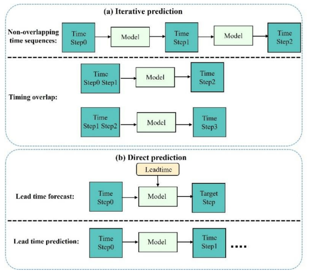
Considering that the prediction strategy directly affects how the model utilizes input information and influences the subsequent evaluation of model structures, this study first compares the forecast performance of different prediction strategies. Existing deep learning-based subseasonal prediction methods can generally be divided into two categories: iterative prediction and direct prediction (Figure 4).

Iterative prediction starts from the current atmospheric state and progressively generates future sequences through rolling recursion. Its advantage is that it more closely resembles the continuous evolution of atmospheric states. However, its limitation is that errors are propagated and gradually accumulated during multi-step recursion, which becomes particularly evident at longer lead times. In contrast, direct prediction does not rely on the prediction result from the previous step, but directly learns the mapping relationship between the current state and the target lead time. This strategy can, to some extent, avoid recursive error accumulation and also has relatively high computational efficiency. Based on this, the different prediction strategies were compared using their mean prediction skill over Weeks 1–6 to determine a temporal modeling strategy more suitable for subseasonal 2-m temperature prediction over East Asia.

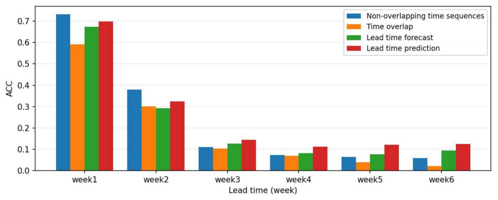
Figure 5 presents the mean ACC results of different prediction strategies for subseasonal 2-m temperature prediction over East Asia during the evaluation period from 2019 to 2024. To ensure a fair comparison, all experiments used the same model structure, input variables, and training strategy, with only the prediction strategy being changed. Overall, the prediction skill of all four strategies decreases markedly with increasing lead time, indicating that the predictable signals of 2-m temperature on the subseasonal time scale decay rapidly over time. However, different temporal-evolution modeling strategies show clear differences in their ability to maintain prediction skill.

The iterative and direct prediction strategies exhibit distinct lead-time-dependent characteristics. Iterative prediction progressively generates future states through rolling recursion, which is closer to the continuous evolution process of atmospheric states, and therefore performs relatively well at short lead times. Among them, the temporally non-overlapping iterative prediction strategy performs best during Weeks 1–2, with ACC values of approximately 0.73 and 0.38, respectively, which are clearly higher than those of the other methods. This indicates that this strategy can more effectively utilize neighboring state information and better capture short-term persistence characteristics. However, as the lead time increases, its prediction skill declines rapidly, reaching only about 0.06 by Week 6. This suggests that error accumulation caused by multi-step recursion clearly limits its medium- and extended-range prediction skill. In contrast, the temporally overlapping iterative prediction strategy shows the weakest overall performance, especially during Weeks 5–6, when the ACC decreases to approximately 0.04 and 0.02, respectively. This indicates that high-frequency rolling recursion is more likely to amplify local errors and is unfavorable for the stable extraction of subseasonal low-frequency signals.

Compared with iterative prediction, direct prediction shows better stability in the medium- and extended-range stages. Lead-time prompted prediction has slightly lower skill than the optimal method during Weeks 1–4, but its rate of skill decline is relatively slow, and it still maintains positive skill of approximately 0.09 by Week 6. Lead-time simultaneous prediction achieves the best overall performance, especially during Weeks 3–6, when it achieves higher ACC than the other prediction strategies. This suggests that direct prediction can, to some extent, avoid recursive error propagation and may better support the learning of slowly varying background signals associated with different target weeks. Overall, iterative prediction is more suitable for short-lead prediction tasks, whereas direct prediction has greater advantages for medium- and extended-range forecasts during Weeks 3–6. Since this study focuses on improving subseasonal prediction skill during Weeks 3–6, the subsequent experiments adopt the lead-time simultaneous prediction strategy with the best overall performance as the basic prediction framework; that is, forecasts for Weeks 1–6 are generated simultaneously through a single forward pass.

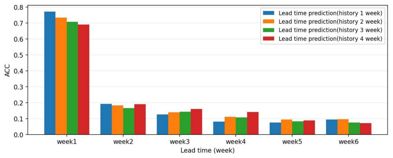
Based on the selected prediction strategy, the influence of different historical input lengths on model performance is further analyzed to clarify the model’s ability to utilize recent atmospheric states and low-frequency background information. Figure 6 shows the sensitivity experiment results for different historical input lengths under the lead-time simultaneous prediction framework, where h1–h4 represent historical information from the previous 1–4 weeks, respectively. The results indicate that a longer historical input does not necessarily lead to better performance; instead, the optimal historical input length varies with the target lead time. For Week 1 prediction, h1 performs best, with an ACC of approximately 0.77. As the historical window increases to h4, the skill decreases to approximately 0.69. This suggests that short-lead prediction mainly depends on recent atmospheric state information, while an excessively long history may introduce additional background differences and weaken the model’s response to the current dominant signals. During Weeks 3–4, however, longer historical windows provide clearer benefits. Among them, h4 achieves the highest skill, with ACC values of approximately 0.16 and 0.14 for Weeks 3 and 4, respectively, which are higher than the corresponding h1 values of approximately 0.12 and 0.08. This indicates that medium-range prediction relies more on the cumulative representation of low-frequency and slowly varying processes, and that appropriately extending the historical input length helps enhance the model’s ability to extract subseasonal predictable signals.

However, during Weeks 5–6, the benefit of increasing the historical input length diminishes and may even reverse. In Week 5, h2 performs slightly better, while in Week 6, h1 and h2 are relatively more stable, whereas h3 and h4 show decreased skill. This suggests that at longer lead times, although a longer historical window can provide more background information, it may also introduce irrelevant noise and redundant signals, thereby weakening the model’s generalization performance. Overall, the optimal historical input length varies clearly among different lead times: shorter historical inputs are more suitable for short-range forecasts, whereas longer historical inputs are more beneficial for medium-range prediction during Weeks 3–4. Although the 4-week historical input achieves better ACC during Weeks 3–4, it does not provide a consistent advantage across all lead weeks. In particular, its skill decreases during Weeks 5–6, suggesting that longer historical windows may introduce redundant or less relevant information at longer lead times. Therefore, the one-week historical input was retained as the default setting as a conservative and unified configuration for the following model-comparison experiments. This choice also reduces computational cost and memory consumption, which is important under the current experimental conditions. This setting is not intended to be optimal for every lead week; rather, it provides a consistent baseline for comparing input variables, model components, and CFSv2 under the same input-length condition.

3.2. Feature Ablation Experiments

After the prediction strategy was selected, feature-ablation experiments were conducted to examine the effects of different input-variable combinations on model performance. SwinUNet-AR was used as the common backbone in all experiments. The experiments differed only in their input-variable configurations. Specifically, the experiments began with a univariate setting using only T2m as input to evaluate the basic predictability of the near-surface temperature field itself. Vertical temperature information was then gradually introduced to examine the contribution of thermal features to subseasonal prediction. On this basis, dynamical and circulation-related factors, including wind fields, geopotential height, relative humidity, and surface pressure, were further added to construct multiple variable-combination schemes (

Table 3. Configuration of the ablation experiments.

Experiment	Model Input Variables	Number of Input Variables
T2m	T2m	1
T	T2m + T850, T500, T200	4
T-UV10	T + U10, V10	6
TUV	T-UV10 + U850, U500, U200 + V850, V500, V200	12
TUVZ	TUV + Z850, Z500, Z200	15
TUVZR	TUVZ + Rh850, Rh500, Rh200	18
ALL	TUVZR + SP	19

), and their prediction performance at different lead weeks was compared. Through this design, the incremental contributions of different predictor groups to the model’s medium- and extended-range prediction skill can be systematically evaluated, providing a basis for determining the default input configuration in subsequent experiments.

Table 4. Mean ACC values of the input-variable ablation experiments. The cumulative ACC is the sum of the mean ACC values for Weeks 3–6. Values are rounded to three decimal places.

Experiment	Week 3	Week 4	Week 5	Week 6	Cumulative ACC (Weeks 3–6)
T2m	0.178	0.144	0.128	0.104	0.554
T	0.197	0.159	0.134	0.107	0.597
T-UV10	0.193	0.159	0.134	0.107	0.593
TUV	0.198	0.158	0.136	0.111	0.603
TUVZ	0.199	0.162	0.138	0.105	0.604
TUVZR	0.201	0.158	0.139	0.114	0.612
ALL	0.200	0.163	0.142	0.118	0.621

presents the mean ACC results for subseasonal 2-m temperature prediction over East Asia during Weeks 3–6 under different meteorological-variable input configurations. To ensure a fair comparison, all experiments use the same model architecture and training strategy, with only the input-variable combination being changed, so as to quantify the contribution of different predictors to medium- and extended-range forecast skill. Overall, as the input variables are gradually expanded from a single near-surface temperature field to multivariable combinations containing thermal, dynamical, and circulation information, the prediction skill of the model during Weeks 3–6 generally increases. However, the gains associated with adding different variables are not strictly monotonic. The full-variable input scheme (ALL) achieves the best performance, with a cumulative ACC of 0.621 during Weeks 3–6, which is 0.067 higher than that obtained using only T2m. This indicates that multisource meteorological information can effectively enhance the model’s ability to extract predictable signals in the medium- and extended-range stages.

In terms of the role of different variable combinations, the ACC values at all lead weeks are lowest when only T2m is used, indicating that a single near-surface state is insufficient to fully represent the large-scale low-frequency background on which subseasonal temperature-anomaly evolution depends. After introducing vertical temperature information, the model skill improves markedly. The cumulative ACC of the T scheme during Weeks 3–6 increases to 0.597, suggesting that thermal-structure information can provide a more stable background constraint for prediction after Week 3. When wind-field variables are further added, the model performance shows a modest further improvement. For example, the cumulative ACC of the TUV scheme reaches 0.603, although the increase is relatively limited. This indicates that dynamical information contributes mainly through its synergistic representation with thermal structures rather than independently determining the forecast performance.

After further adding geopotential height and relative humidity, the model performance continues to improve. The cumulative ACC values of the TUVZ and TUVZR schemes reach 0.604 and 0.612, respectively, indicating that large-scale circulation patterns and humidity-related processes provide additional constraints for medium- and extended-range prediction. In particular, humidity information contributes more clearly to the improvement of Week 6 skill. Finally, the ALL scheme achieves the best performance, with the largest gains occurring during Weeks 4–6. This suggests that the complete variable combination not only improves the overall prediction skill, but also more effectively suppresses skill degradation at longer lead times. Overall, multivariable input can significantly improve subseasonal 2-m temperature prediction over East Asia. Among the input variables, vertical thermal-structure information provides the largest incremental contribution under the present sequential-addition design, while wind fields, geopotential height, and humidity variables offer further complementary constraints. Based on forecast skill and stability, the ALL scheme is adopted as the default input configuration in subsequent experiments. When input dimensionality and computational efficiency are also considered, TUVZR can be regarded as an alternative scheme with performance close to the optimum.

From a physical perspective, the feature-ablation results provide a preliminary indication of the incremental contributions of different predictor groups under the specified addition order. The improvement from T2m to T suggests that vertical thermal-structure information provides a larger incremental gain than near-surface temperature alone under the present addition order for Weeks 3–6 prediction. The further improvement after adding wind fields and geopotential height indicates that large-scale dynamical circulation and temperature advection provide additional predictive information. The increase after adding relative humidity and surface pressure suggests that moisture-related processes and near-surface pressure conditions also contribute to the maintenance of subseasonal temperature anomalies. Therefore, the model skill is not only derived from local temperature persistence, but also from the combined representation of thermal, dynamical, circulation, and moisture-related background conditions.

3.3. Module Ablation Results

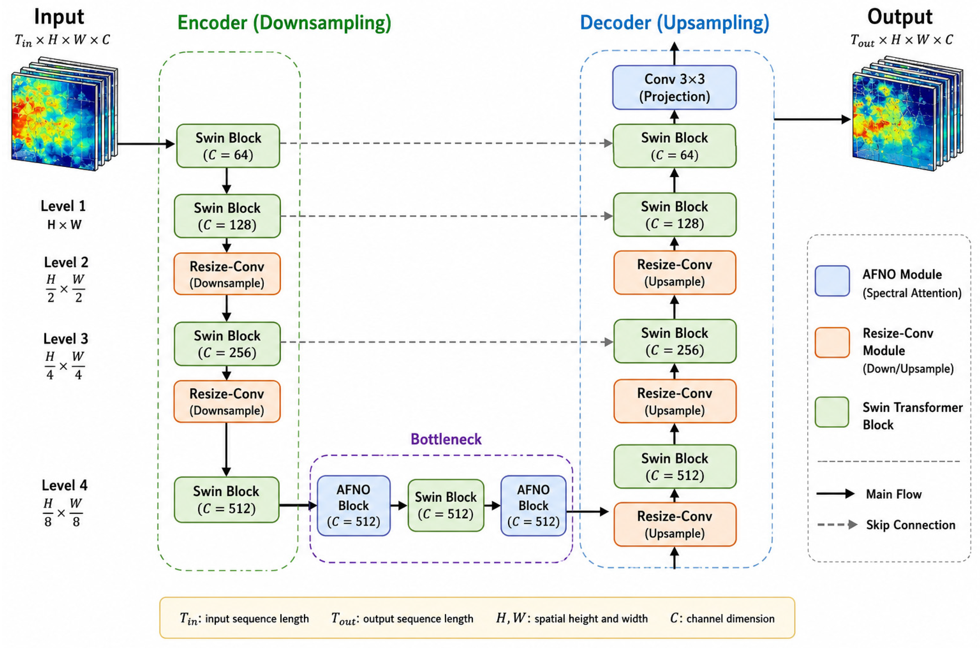
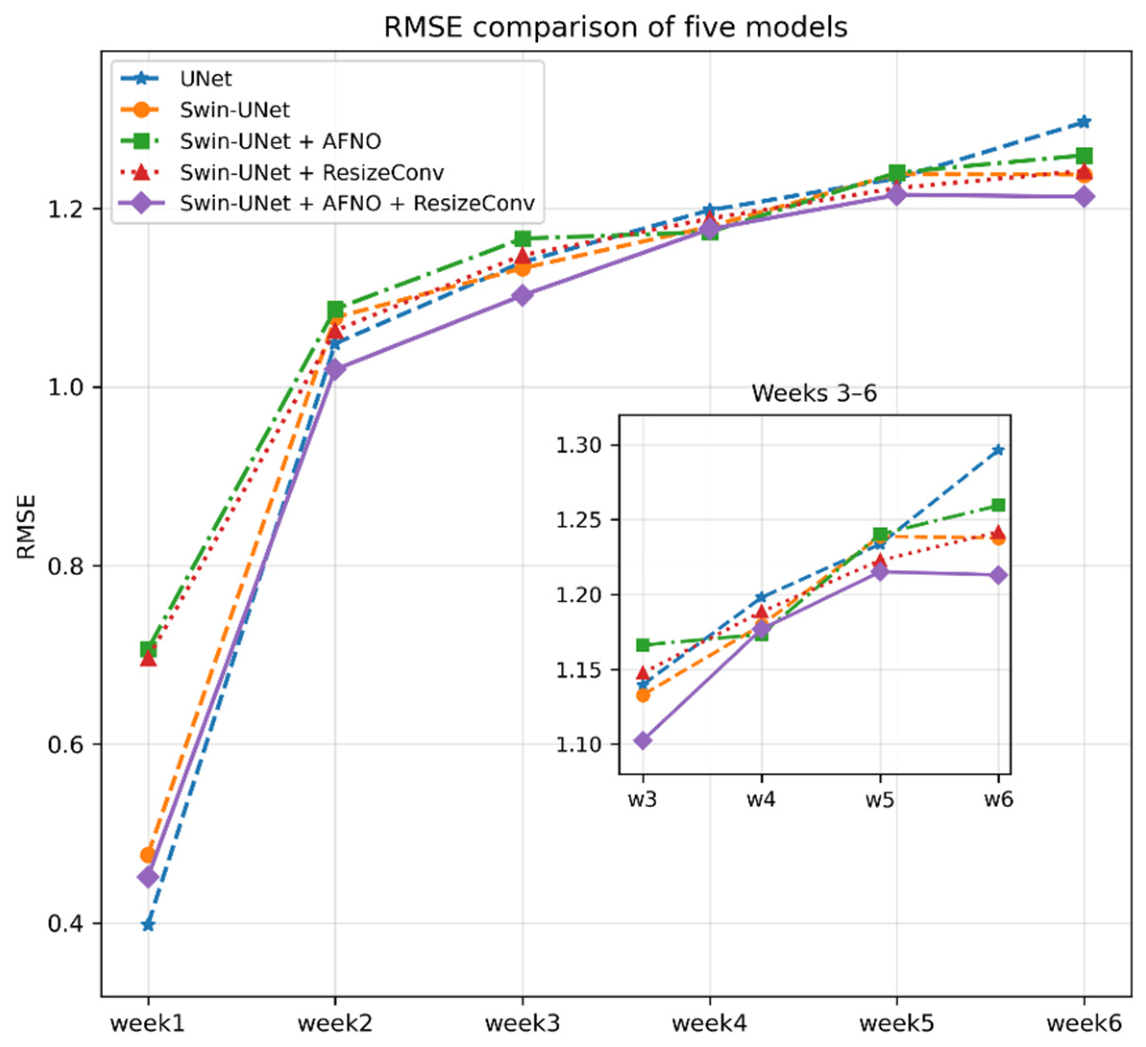
Based on the selected prediction strategy and input-variable combination, module-ablation experiments were then designed to evaluate the effects of the proposed architectural modifications. The baseline SwinUNet was used as the control model. Several comparative configurations were constructed by adding or removing AFNO and Resize-Conv from the baseline SwinUNet. All experiments adopted the same dataset split, input-variable configuration, training epochs, and optimization parameters. Differences in forecast skill among the model configurations for Weeks 1–6 were first compared using the RMSE curves shown in Figure 7. To further summarize the medium- and extended-range performance quantitatively,

Table 5. Results of the module ablation experiments.

AFNO	Resize-Conv	Mean RMSE (Weeks 3–4)	Mean RMSE (Weeks 5–6)	Cumulative ACC (Weeks 3–6)
×	×	1.16 °C	1.24 °C	0.58
√	×	1.17 °C	1.25 °C	0.57
×	√	1.17 °C	1.23 °C	0.58
√	√	1.14 °C	1.21 °C	0.62

Note: √ indicates that the corresponding module is included in the model, whereas × indicates that the corresponding module is not included. Bold values indicate the best performance among all module-ablation configurations.

presents the mean RMSE values for Weeks 3–4 and Weeks 5–6, together with the cumulative ACC for Weeks 3–6.

Overall, the RMSE values of the five models increase markedly with lead time, indicating that forecast errors in 2-m temperature prediction generally increase as the forecast range extends from Week 1 to Week 6. The RMSE values of all models are relatively low in Week 1, suggesting that short-lead prediction is mainly constrained by initial-condition information and short-term atmospheric persistence, and performance differences among the model architectures remain small. From Week 3 onward, structural differences among the models become more apparent as forecast errors increase. At this stage, differences among network structures in representing low-frequency background signals, improving spatial reconstruction quality, and suppressing error accumulation become more evident.

The week-by-week RMSE curves show that UNet achieves the lowest RMSE in Week 1, with a value of 0.40 °C, indicating that a simple convolutional structure can effectively capture short-term local temperature persistence at short lead times. However, as the lead time increases, the RMSE of UNet increases rapidly, reaching 1.30 °C in Week 6. This indicates its limited ability to maintain slowly varying signals and large-scale anomalous structures in the medium- and extended-range stages. The baseline SwinUNet shows more stable performance than UNet during Weeks 3–6, with the Week 6 RMSE decreasing to 1.24 °C. This suggests that the introduction of a hierarchical window-attention structure enhances the model’s ability to represent multiscale spatial features.

Further comparison of different modules shows that, when only the AFNO module is added, the RMSE values in Weeks 1 and 2 are 0.71 °C and 1.09 °C, respectively, which are higher than those of the baseline SwinUNet. In addition, no stable advantage is observed during Weeks 3–6. This indicates that, although the frequency-domain module extracts large-scale spectral features, the additional processing does not translate into lower overall RMSE under the present configuration without sufficient recovery of spatial detail in the decoder.

The Resize-Conv-only configuration generally yields slightly lower RMSE than the AFNO-only configuration during Weeks 3–6, with the clearest difference occurring during Weeks 5–6. When AFNO and Resize-Conv are introduced simultaneously, the model achieves among the lowest RMSE values in the medium- and extended-range stages. The RMSE values of SwinUNet + AFNO + ResizeConv from Weeks 2 to 6 are 1.02 °C, 1.10 °C, 1.18 °C, 1.22 °C, and 1.21 °C, respectively, which are generally lower than those of the baseline SwinUNet and the single-module schemes. In particular, during Weeks 3–6, the RMSE curve of this model remains at a relatively low level, indicating a certain complementarity between the large-scale low-frequency signal modeling capability of AFNO and the spatial reconstruction capability of Resize-Conv. The combined configuration yields lower RMSE and higher cumulative ACC than either single-module configuration, suggesting that AFNO and Resize-Conv may provide complementary benefits under the present architecture.

Table 5 further presents the mean RMSE values of different module combinations during Weeks 3–4 and Weeks 5–6, as well as the cumulative ACC during Weeks 3–6. The baseline SwinUNet has RMSE values of 1.16 °C and 1.24 °C during Weeks 3–4 and Weeks 5–6, respectively, indicating that error accumulation at longer lead times remains an important factor limiting the model’s medium- and extended-range prediction skill. After adding only AFNO, the RMSE values in the two time windows are 1.17 °C and 1.25 °C, respectively, which are not lower than those of the baseline SwinUNet. This suggests that AFNO alone does not reduce RMSE relative to the baseline under the present configuration. After adding only Resize-Conv, the RMSE values during Weeks 3–4 and Weeks 5–6 are 1.17 °C and 1.23 °C, respectively. The RMSE during Weeks 5–6 is slightly lower than that of the baseline SwinUNet, indicating that this module can partly alleviate spatial reconstruction errors at longer lead times. By contrast, when AFNO and Resize-Conv are added simultaneously, the RMSE values during Weeks 3–4 and Weeks 5–6 decrease to 1.14 °C and 1.21 °C, respectively, both of which are the lowest among all ablation schemes. Meanwhile, the cumulative ACC during Weeks 3–6 increases to 0.62, indicating that the dual-module combination not only reduces the magnitude of prediction errors but also improves the consistency of anomalous spatial patterns.

Overall, AFNO does not consistently reduce RMSE when used alone, whereas the combined AFNO-Resize-Conv configuration yields lower RMSE and higher cumulative ACC than either single-module configuration. Resize-Conv helps improve the spatial reconstruction quality in the decoding stage and reduces error propagation that may be caused by the upsampling process. The resulting SwinUNet-AR, which combines both modules, shows lower RMSE and higher cumulative ACC during the medium- and extended-range period of Weeks 3–6. These results indicate that the proposed module combination improves the stability and accuracy of medium- and extended-range subseasonal 2-m temperature prediction under the present experimental setting.

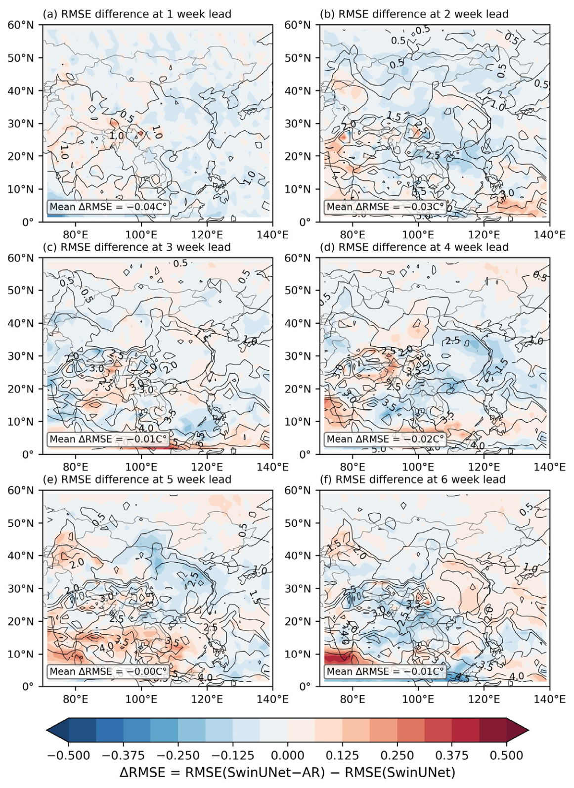
Figure 8 further shows the spatial distribution of RMSE differences between SwinUNet-AR and the baseline SwinUNet at different lead times. The shading represents the RMSE difference between the two models, namely ΔRMSE = RMSE(SwinUNet-AR) − RMSE(SwinUNet), while the contours indicate the spatial distribution of RMSE for SwinUNet-AR itself. The figure further illustrates the spatial characteristics of the error differences between the improved and baseline models and their evolution with lead time.

Overall, the shaded fields at different lead times are dominated by small positive and negative differences close to zero, but negative values prevail over most regions. This indicates that SwinUNet-AR can reduce prediction errors to some extent in most areas of East Asia. The regional mean ΔRMSE values shown in the subplots are −0.04 °C, −0.03 °C, −0.01 °C, −0.02 °C, −0.00 °C, and −0.01 °C, respectively. These results suggest that, compared with the baseline SwinUNet, SwinUNet-AR achieves slight but relatively stable RMSE improvements over Weeks 1–6, with more evident average improvements in Weeks 1–2 and Week 4.

From the spatial distributions at different lead times, the differences between the two models are generally small during Weeks 1–2. The shaded fields mainly consist of scattered weak negative values and localized weak positive values, indicating that short-lead prediction is still mainly constrained by the initial atmospheric state, and the error reduction brought by structural improvements has not yet fully emerged. Nevertheless, SwinUNet-AR already exhibits a certain range of negative ΔRMSE values over parts of the mid- and low-latitude regions of East Asia and surrounding areas, suggesting that the improved structure has begun to suppress errors even at short lead times.

As the lead time extends to Weeks 3–6, the differences between the two models become clearer. Although a few localized regions still show positive ΔRMSE, negative ΔRMSE values are more widely distributed over key mid- and low-latitude regions of East Asia, South Asia, and adjacent oceanic areas. This indicates that SwinUNet-AR can maintain lower forecast errors over more regions during the medium- and extended-range stages. Meanwhile, the contours show that the RMSE of SwinUNet-AR generally increases with lead time, and high-error regions gradually expand toward low-latitude areas and regions with complex circulation activity. This is consistent with the general pattern of error accumulation with increasing lead time in subseasonal prediction. Although the overall RMSE increases in the medium- and extended-range stages, SwinUNet-AR still generally maintains slightly lower RMSE than the baseline SwinUNet, indicating that the improved structure can partly buffer and suppress error accumulation.

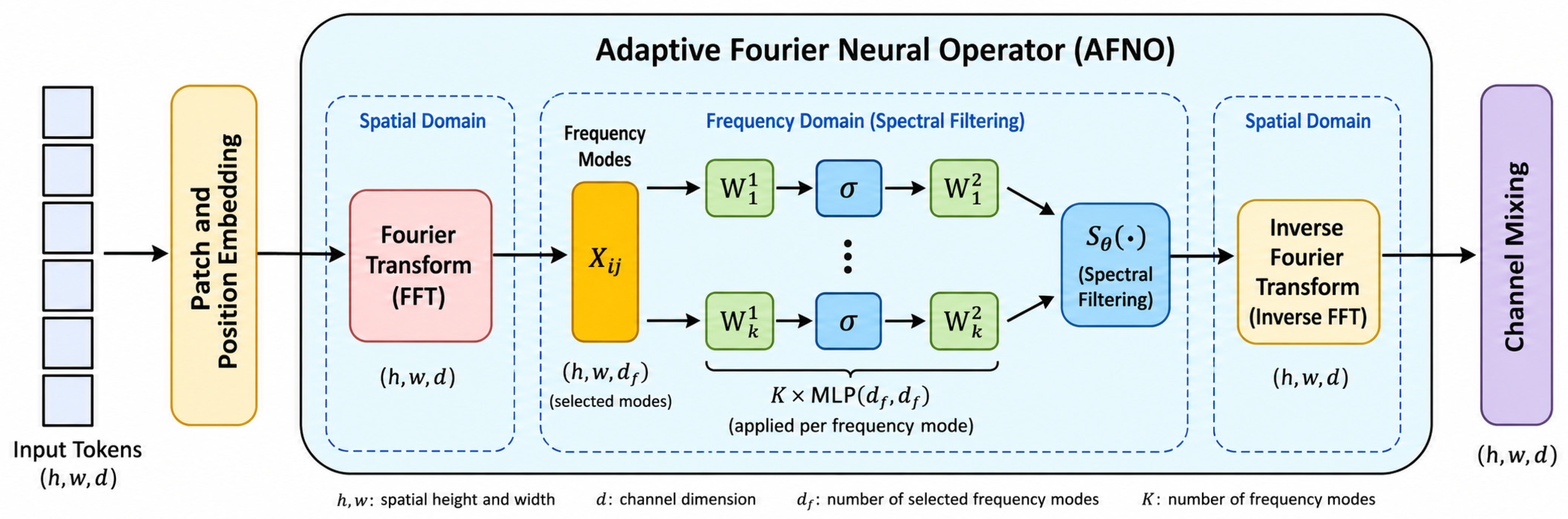
Taken together, Figure 7 and Figure 8 show that SwinUNet-AR generally yields slightly lower RMSE than the baseline SwinUNet, although the improvements are modest and spatially heterogeneous. Its advantage is reflected not only in the reduction of mean RMSE during the medium- and extended-range stages, but also in the broader distribution of negative ΔRMSE values across most regional error fields. The AFNO module enhances the direct modeling of large-scale low-frequency background signals at the bottleneck layer, thereby improving the model’s ability to represent cross-regional coherent anomalous structures. Resize-Conv improves the quality of spatial reconstruction in the decoding stage and reduces local artifacts and upsampling errors. These two modules jointly improve model performance from the key aspects of feature extraction and output recovery, providing modest improvements in error control and spatial continuity under the present experimental setting.

3.4. Comparative Evaluation of SwinUNet-AR and CFSv2

The final SwinUNet-AR model was further compared with CFSv2 to evaluate its subseasonal forecast performance over East Asia. CFSv2 is a widely used coupled dynamical prediction system. It can simulate atmospheric circulation evolution based on physical processes and provide subseasonal forecast products. Comparing SwinUNet-AR with CFSv2 helps assess the advantages and limitations of the regional deep learning model relative to the dynamical prediction system in subseasonal 2-m temperature prediction over East Asia. Before the comparison, the CFSv2 forecasts were processed to match the verification framework of SwinUNet-AR as closely as possible. The original 6-hourly CFSv2 forecasts were averaged into daily means, and the 32 ensemble members were averaged to obtain the ensemble-mean forecast. The daily CFSv2 forecasts were then aggregated into the same lead-week windows as the SwinUNet-AR targets. Both systems were evaluated over the same East Asian domain, on the same 1.5° × 1.5° grid, and against ERA5 as the verifying reference. RMSE was calculated using weekly mean 2-m temperature fields, while ACC was calculated using weekly mean anomaly fields after removing the corresponding lead-dependent climatological mean. This consistent preprocessing and verification framework was used to reduce differences caused by temporal aggregation, spatial resolution, and anomaly definition. However, the CFSv2 forecasts were used as raw model outputs without additional bias correction. Therefore, the RMSE comparison should be interpreted as a comparison between SwinUNet-AR and raw CFSv2 forecasts, and part of the RMSE difference may be associated with the systematic climatological bias of CFSv2. 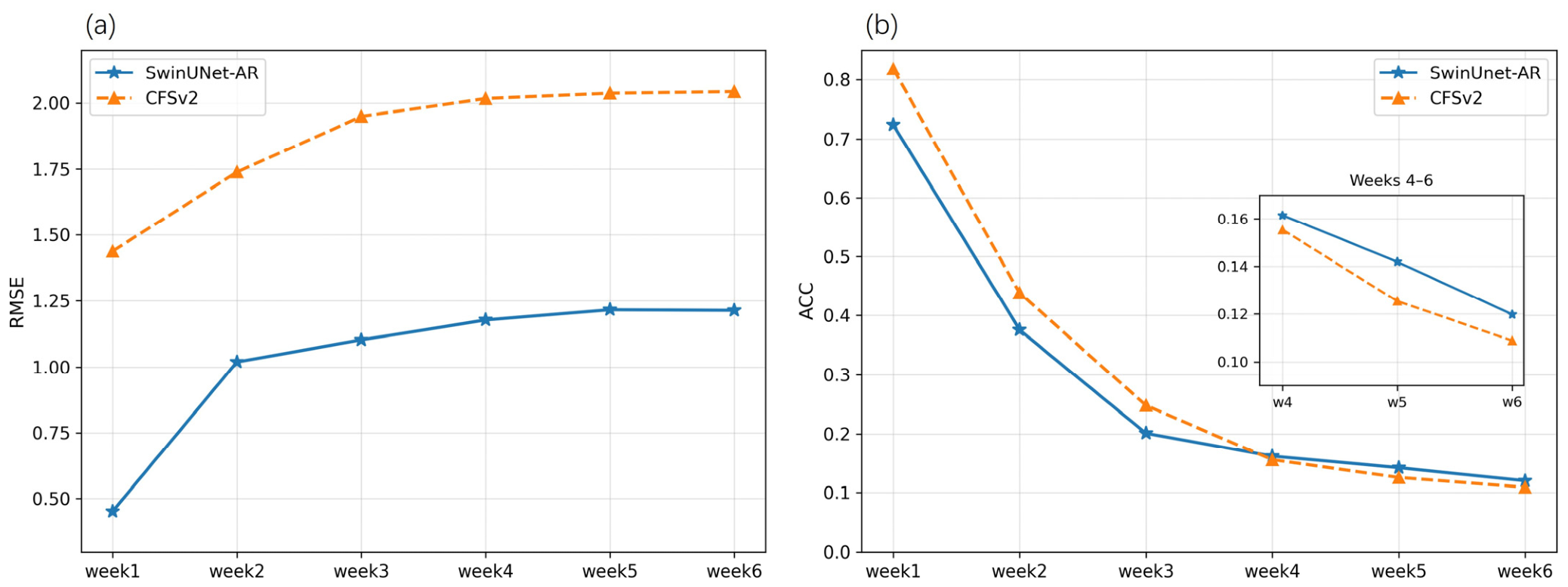Figure 9 shows the comparison of RMSE and ACC between SwinUNet-AR and CFSv2 for Lead Weeks 1–6.

In terms of RMSE, both systems show increasing errors with lead time. Under the present verification framework, SwinUNet-AR shows lower RMSE than raw CFSv2 at all lead weeks. Specifically, the RMSE of CFSv2 increases from 1.437 °C in Week 1 to 2.04 °C in Week 6, with a mean RMSE of approximately 1.87 °C over Weeks 1–6. In comparison, the RMSE of SwinUNet-AR increases from 0.45 °C in Week 1 to 1.21 °C in Week 6, with a mean RMSE of approximately 1.03 °C. However, this RMSE difference should be interpreted cautiously because CFSv2 was evaluated using raw ensemble-mean forecasts without additional bias correction, whereas SwinUNet-AR was trained directly against ERA5. Therefore, the lower RMSE of SwinUNet-AR reflects both lower forecast errors and the model’s ability to fit the ERA5-based temperature distribution and should not be regarded as a fully bias-corrected operational comparison.

In terms of ACC, the comparison is based on climatological anomalies and is therefore less affected by mean-state bias. CFSv2 shows higher ACC during Weeks 1–3, indicating that the dynamical model retains advantages in representing physically consistent anomaly evolution at short to medium lead times. During Weeks 4–6, SwinUNet-AR becomes more competitive and shows slightly higher ACC than CFSv2 at some lead times. However, the ACC difference is relatively small and should be interpreted cautiously. Overall, the CFSv2 comparison should be viewed as a reference benchmark rather than as direct evidence that the data-driven model fully outperforms the dynamical system. These results suggest that SwinUNet-AR may provide a useful regional complement to dynamical forecasts, particularly in achieving lower RMSE than raw CFSv2 forecasts, while CFSv2 still retains advantages in short-lead anomaly-pattern prediction.

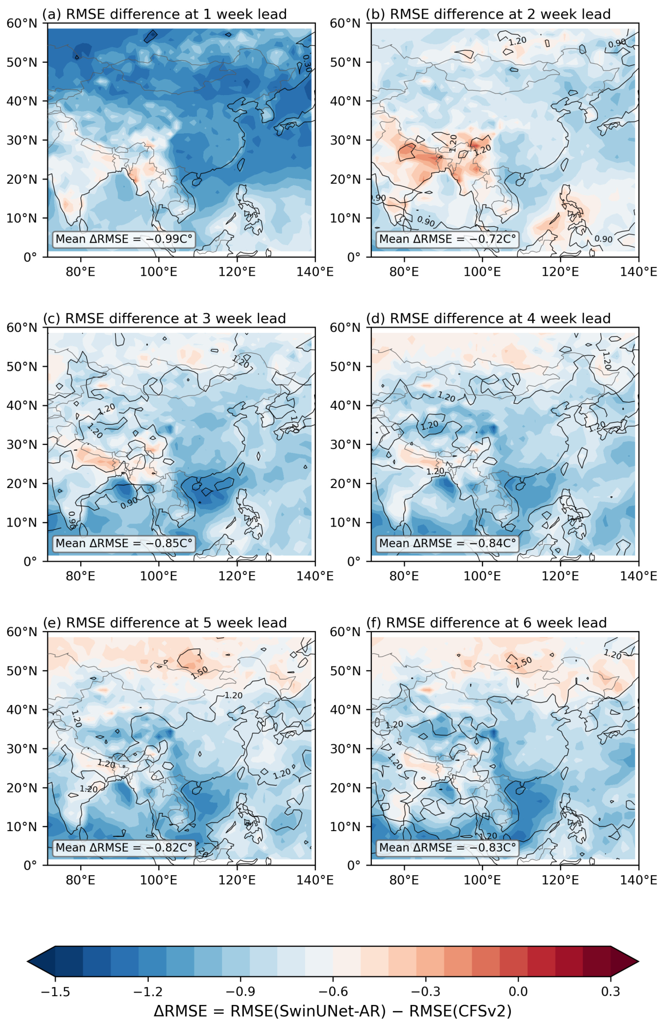
To further analyze the differences in the spatial error distributions between SwinUNet-AR and the dynamical model CFSv2, Figure 10 shows the spatial distribution of RMSE differences between the two models at different lead times. The regional mean ΔRMSE values for Weeks 1–6 are all negative, at approximately −0.99, −0.72, −0.85, −0.84, −0.82, and −0.83 °C, respectively. Because ΔRMSE is defined as RMSE(SwinUNet-AR) − RMSE(CFSv2), these negative values indicate that SwinUNet-AR has lower RMSE than raw CFSv2 at all lead times under the present verification framework. The largest difference occurs in Week 1, when the RMSE of SwinUNet-AR is approximately 0.99 °C lower than that of CFSv2. During Weeks 2–6, the regional mean differences remain between approximately −0.72 and −0.85 °C. However, because CFSv2 was evaluated without additional bias correction, these differences reflect both forecast errors and mean-state biases and should not be interpreted as evidence that SwinUNet-AR comprehensively outperforms the dynamical forecasting system.

From a spatial perspective, most regions in Figure 10 are dominated by blue shading, indicating that the RMSE of SwinUNet-AR is lower than that of CFSv2 at most grid points over East Asia. During Weeks 1–2, the negative-value regions are widely distributed, suggesting that SwinUNet-AR has lower RMSE than raw CFSv2 over most grid points in the verification domain at short lead times. By Weeks 3–6, the blue-shaded regions still persist over a large area, indicating that even in the medium- and extended-range subseasonal stage, SwinUNet-AR continues to exhibit lower RMSE than raw CFSv2 across most regions. The localized red regions indicate that, in some areas and at certain lead times, the RMSE of CFSv2 may be lower than that of SwinUNet-AR. These localized positive differences indicate regional and lead-dependent variations in relative model performance; their physical causes require further investigation.

The RMSE contours for SwinUNet-AR show that its error level generally increases with lead time. The contour values are relatively low in Week 1, indicating that SwinUNet-AR shows relatively low RMSE against ERA5 at short lead times. As the lead time extends to Weeks 3–6, the area covered by higher RMSE contours gradually expands, reflecting the typical increase in forecast error with lead time in subseasonal prediction. Nevertheless, the shaded differences are still dominated by negative values, indicating that although the RMSE of SwinUNet-AR increases with lead time, it still maintains a lower error level than CFSv2.

Taken together, Figure 9 and Figure 10 show that SwinUNet-AR has consistently lower RMSE than raw CFSv2 under the present verification framework. However, part of this RMSE difference may reflect the mean-state bias of the uncorrected CFSv2 forecasts. The results therefore suggest that SwinUNet-AR may serve as a useful regional complement to dynamical subseasonal forecasts.

3.5. Statistical Significance of Model Improvements

Table 6. Statistical significance of the main model improvements.

Comparison	Period	Metric	Mean Improvement	95% CI	Significant
ALL vs. T2m	Weeks 3–6	ACC sum	0.067	[0.031, 0.102]	Yes
SwinUNet-AR vs. SwinUNet	Weeks 3–4	RMSE	0.020 °C	[−0.004, 0.043]	No
SwinUNet-AR vs. SwinUNet	Weeks 5–6	RMSE	0.030 °C	[0.002, 0.057]	Yes
SwinUNet-AR vs. SwinUNet	Weeks 3–6	ACC sum	0.040	[0.006, 0.074]	Yes
SwinUNet-AR vs. raw CFSv2	Weeks 1–6	RMSE	0.840 °C	[0.765, 0.918]	Yes
SwinUNet-AR vs. raw CFSv2	Weeks 4–6	RMSE	0.830 °C	[0.742, 0.921]	Yes
SwinUNet-AR vs. CFSv2	Weeks 4–6	ACC	0.012	[−0.003, 0.028]	No

summarizes the statistical significance of the main model improvements. The ALL input scheme shows a statistically significant cumulative ACC improvement over the T2m-only scheme during Weeks 3–6, indicating that the use of multivariable atmospheric information provides a statistically robust improvement in forecast skill. For the module ablation experiments, SwinUNet-AR improves the cumulative ACC during Weeks 3–6 compared with the baseline SwinUNet, and the corresponding confidence interval does not include zero. However, the RMSE reductions are relatively small. The RMSE improvement during Weeks 3–4 is not statistically significant, whereas the improvement during Weeks 5–6 is statistically significant but small in magnitude. Therefore, the structural advantage of SwinUNet-AR should be interpreted mainly as a modest improvement in medium- and extended-range prediction stability and anomaly-pattern consistency. Compared with raw CFSv2 forecasts, SwinUNet-AR shows statistically significant RMSE reductions, but the ACC improvement during Weeks 4–6 is small and not statistically significant.

4. Discussion

This section interprets the main findings of this study in relation to subseasonal predictability, data-driven weather forecasting, and dynamical prediction systems. The results show that prediction skill decreases rapidly from Week 1 to Week 6, which is consistent with the well-known difficulty of subseasonal prediction. At short lead times, forecasts still benefit from atmospheric persistence and initial-condition information. This explains why the temporally non-overlapping iterative strategy performs well during Weeks 1–2. However, as the lead time increases, recursive prediction is more affected by error accumulation. In contrast, lead-time simultaneous prediction avoids part of this recursive error propagation and provides more stable skill during Weeks 3–6, making it more suitable for the medium- and extended-range subseasonal prediction task considered here. This lead-time-dependent decline in prediction skill is broadly consistent with the general challenge of subseasonal prediction discussed by Robertson et al. [34].

The feature ablation results indicate that multivariable input is important for Weeks 3–6 prediction. Compared with using only T2m, the full-variable scheme provides additional thermal, dynamical, circulation, humidity, and surface-pressure information. This is physically reasonable because subseasonal temperature anomalies over East Asia are influenced not only by local near-surface persistence, but also by vertical thermal structure, horizontal temperature advection, mid-tropospheric circulation, land–sea pressure contrast, and moisture-related processes. In particular, upper-air temperature and geopotential height help describe the large-scale thermal and circulation background, wind fields provide information on dynamical transport, and humidity may be related to cloud, radiation, and moisture processes affecting regional temperature anomalies. Therefore, the improvement from multivariable input suggests that the model benefits from broader atmospheric background information rather than relying only on local temperature persistence. Although Zhong and Wu [24] focused specifically on East Asian winter temperature, their results provide a relevant conceptual comparison by highlighting the role of large-scale thermal and circulation modes in subseasonal predictability. In the present study, the improvements obtained after introducing vertical temperature, wind, geopotential height, relative humidity, and surface pressure similarly suggest that T2m prediction benefits from broader atmospheric background information beyond local near-surface persistence.

The module ablation experiments further show that the contributions of AFNO and Resize-Conv appear to be complementary. SwinUNet provides a hierarchical encoder–decoder structure for multiscale spatial feature extraction, but its local-window attention may be insufficient for representing domain-wide low-frequency signals at subseasonal lead times. AFNO is introduced at the bottleneck layer to enhance frequency-domain representation and long-range dependency modeling, which is consistent with the use of Fourier-based neural operators in data-driven weather prediction. However, AFNO alone does not consistently reduce RMSE, suggesting that large-scale spectral mixing does not automatically ensure accurate recovery of local spatial gradients in the final temperature field. The Resize-Conv-only configuration produces slightly more consistent RMSE reductions than the AFNO-only configuration, which is consistent with its intended role in decoder reconstruction. When AFNO and Resize-Conv are used together, the model better balances large-scale signal representation and local spatial reconstruction, leading to the best medium- and extended-range performance in the ablation experiments.

The statistical significance analysis shows that the robustness of the improvements varies across comparisons. The improvement from multivariable input is statistically significant, supporting the importance of large-scale atmospheric background information for East Asian subseasonal temperature prediction. For the module ablation experiments, the cumulative ACC improvement of SwinUNet-AR during Weeks 3–6 is significant, whereas some RMSE reductions are small and not always statistically significant. Therefore, the structural advantage of SwinUNet-AR should be interpreted as a modest improvement in anomaly-pattern consistency and medium- to extended-range prediction stability, rather than as a large breakthrough in deterministic temperature accuracy. From an operational perspective, RMSE reductions of only 0.02–0.04 °C may have limited direct impact, and their practical value should be further assessed using application-oriented metrics and event-based verification.

The comparison with CFSv2 highlights the different strengths of dynamical and data-driven models. CFSv2 retains higher ACC during Weeks 1–3, indicating that dynamical models still have advantages in representing physically consistent anomaly evolution under stronger initial-condition constraints. SwinUNet-AR shows lower RMSE than raw CFSv2 and becomes more competitive in ACC during Weeks 4–6, suggesting that the regional deep learning model can extract useful medium- and extended-range statistical signals from historical reanalysis data under the present verification framework. However, this comparison should be interpreted cautiously. CFSv2 was evaluated using raw forecasts without additional bias correction, whereas SwinUNet-AR was trained directly against ERA5. Therefore, the RMSE advantage of SwinUNet-AR partly reflects its ability to fit the ERA5-based temperature distribution and should not be regarded as a fully bias-corrected operational forecast-skill comparison. The proposed model should therefore be viewed as a potential complement to, rather than a replacement for, dynamical forecasting systems.

These findings are broadly consistent with previous data-driven subseasonal forecasting studies. Xie et al. [35] reported that a deep learning model incorporating scale interactions was less competitive than dynamical models for surface air temperature prediction over China at relatively short lead times but became more competitive beyond approximately 20 days. Similarly, Chen et al. [20] demonstrated that FuXi-S2S achieved competitive T2m anomaly prediction skill during Weeks 3–6, although its relative performance varied with lead time, variable, and region. The present results exhibit a comparable lead-time-dependent transition: CFSv2 retains higher ACC during Weeks 1–3, whereas SwinUNet-AR becomes more competitive during Weeks 4–6. Nevertheless, the present study differs from these previous studies in several respects. Xie et al. [35] focused on surface air temperature and heat-wave prediction over China using a scale-interaction framework, whereas FuXi-S2S is a global subseasonal forecasting system. By contrast, the present study focuses on deterministic weekly mean 2-m temperature prediction over the broader East Asian domain and evaluates a regional architecture combining hierarchical multiscale representation, bottleneck frequency-domain modeling, and artifact-reduced spatial reconstruction.

From an application perspective, SwinUNet-AR is trained offline using GPU resources and generates forecasts for Weeks 1–6 through a single forward pass after training. This design suggests the potential for computationally efficient inference once the required predictor fields are available. However, direct computational-cost comparisons with full dynamical forecasting systems are beyond the scope of the present study. The model may also be updated periodically as new reanalysis or forecast datasets become available. Future application-oriented studies should evaluate training time, inference time, memory consumption, hardware requirements, update frequency, and deployment stability.

Several limitations remain. First, the evaluation mainly reports annual mean skill over the full East Asian domain, and seasonal or subregional differences were not systematically examined. Future work should evaluate performance separately for boreal winter, boreal summer, and the transition seasons, as well as for key subregions such as northern China, eastern China, the Tibetan Plateau, Japan and Korea, and southern monsoon-influenced areas. Second, the model’s applicability to high-impact warm and cold extremes has not been verified using event-based metrics such as hit rate, false alarm ratio, anomaly amplitude, or spatial pattern agreement. Third, the physical interpretability of the model remains limited. Future studies should introduce saliency maps, integrated gradients, SHAP values, or attention visualization to identify influential predictors, key source regions, and possible teleconnection signals such as ENSO, the Arctic Oscillation, and the Madden–Julian Oscillation. Finally, the present validation is based on one chronological train–test split, and additional rolling-origin evaluation, multiple temporal splits, bias-corrected CFSv2 comparisons, and benchmarks such as persistence, climatology, CNN, ConvLSTM, and pure AFNO should be included to further assess model robustness.

5. Conclusions

Overall, SwinUNet-AR shows promising but still limited skill in subseasonal 2-m temperature prediction over East Asia. Compared with raw CFSv2 forecasts, SwinUNet-AR reduces the mean RMSE over Weeks 1–6 by approximately 44.9% and the mean RMSE during Weeks 4–6 by approximately 40.8%. During Weeks 4–6, SwinUNet-AR shows a small mean ACC increase of 0.012 relative to CFSv2, but this difference is not statistically significant. These results suggest that a regional deep learning model specifically designed for subseasonal prediction can serve as a useful complement to traditional dynamical forecasting systems. However, these performance differences should be interpreted cautiously. The ACC values at longer lead times remain relatively low, indicating that extended-range anomaly-pattern prediction over East Asia is still challenging. In addition, because CFSv2 was evaluated using raw forecasts without additional bias correction, whereas SwinUNet-AR was trained directly against ERA5, the RMSE advantage of SwinUNet-AR should not be regarded as a fully bias-corrected operational forecast-skill comparison.

Several limitations should be acknowledged. First, CFSv2 still shows higher ACC during Weeks 1–3, indicating better short-lead anomaly-pattern skill under the present verification framework. Second, the spatial improvements of SwinUNet-AR are heterogeneous, and its performance remains limited in some low-latitude and monsoon-influenced regions. Third, the present evaluation mainly reports annual mean skill over the full East Asian domain, while seasonal and subregional differences were not systematically examined. Fourth, the model’s applicability to high-impact warm and cold extremes still requires event-based verification. Finally, although multivariable input leads to a statistically significant ACC improvement, some RMSE reductions relative to the baseline SwinUNet are small and should not be overinterpreted from an operational perspective. Future work should include seasonal and subregional verification, rolling-origin evaluation, multiple temporal splits, comparisons with additional benchmarks such as persistence, climatology, CNN, ConvLSTM, pure AFNO, and bias-corrected CFSv2, as well as interpretability analyses and extreme-event-oriented metrics to further assess the robustness and practical value of SwinUNet-AR.