Enhanced Speed Control of PMSM Using Sliding Mode Controller Optimized by Chess Optimization Algorithm

Abstract

This paper introduces an enhanced speed control strategy for permanent magnet synchronous motors (PMSMs) through the application of sliding mode control (SMC) optimized by the Chess Optimization Algorithm (COA). Additionally, the proposed method is compared with other validated algorithms, such as Harris Hawk Optimization (HHO) and the Whale Optimization Algorithm (WOA). The SMC parameters are optimized using Integral of Time-weighted Absolute Error (ITAE) and Integral of Time-weighted Square Error (ITSE) as objectives function, and the controllers are validated in MATLAB/Simulink analyzing transient response, speed variation, and load disturbance conditions. The results show that COA-tuned SMC provides better performance, with the lowest overshoot of 0.1929% for ITAE and 3.4800% for ITSE, the fastest settling times of 0.00307 s for ITSE, and the lowest MAE and RMSE in most evaluated scenarios, offering the most balanced overall performance among the optimization algorithms tested. Comparison to PI and PID controllers demonstrates that SMC provides enhanced accuracy, robustness, and disturbance rejection. COA-SMC provides an efficient and stable solution for PMSM applications that demand quick and accurate speed regulation.

1. Introduction

In the last ten years, people worldwide have become more worried about climate change, air pollution in cities, and the rapid depletion of fossil fuel reserves. These problems are all connected, which has sped up the move toward cleaner and more sustainable energy systems, especially in the transportation sector, which is responsible for the most greenhouse gas emissions [1]. Conventional internal combustion vehicles still release large amounts of ${\mathrm{CO}}_2$ and other harmful pollutants, putting both the environment and public health at risk. Consequently, electric vehicles (EVs) have become an important solution because they do not emit any harmful gasses and can work with renewable energy sources for a long time [2,3]. As a result, many countries, such as Thailand, have stepped up their research and development in electric propulsion technologies, especially in electric motor systems, which are very important for converting electrical power into mechanical motion.

Permanent magnet synchronous motors (PMSMs) are currently the most popular type of motor used in electric vehicles (EVs) and industrial automation because they are very efficient, with better torque density and dynamic performance than induction or brushed DC motors [4]. Even with these benefits, PMSM performance can be affected by changes in parameters, such as resistance changes that depend on temperature, magnetic flux weakening, or load disturbances. These uncertainties can make motors less efficient and traditional control methods less accurate [5,6].

Sliding mode control (SMC) is an established method to deal with nonlinear systems and reduce the importance of changes in parameters and outside forces [7]. It is a good choice for PMSM drives that operate in uncertain or rapidly changing situations because the controller is robust [8,9,10,11]. However, one problem with SMC is that it can cause chattering, which occurs when the control signal oscillates at high frequencies because of rapid switching near the sliding surface [12]. Chattering not only makes it difficult to control the smoothness of the motion, but it may also harm motor performance and damage parts that are sensitive. To avoid this disadvantage, while maintaining the fast dynamic properties of the system, continuous sliding mode alternatives have been widely investigated in the modern literature. For instance, improved continuous terminal sliding mode position control frameworks have been applied to PMSM servo systems to reduce chattering while strictly respecting operational speed and current limits [13]. Moreover, advanced designs merging critical current-constrained continuous nonsingular terminal sliding mode control with control barrier functions (CBFs) have exhibited great success in smoothing out high-frequency control ripples and guaranteeing circuitry safety under severe multi-source uncertainties [14]. While these continuous architectures offer high tracking precision, they often introduce complex derivative terms and heavy computational burdens. As an alternative, this paper utilizes a boundary layer interpolation method via a saturation function, optimized via a metaheuristic framework to balance execution simplicity with robust chattering rejection.

Metaheuristic algorithms have recently become popular for optimizing controller parameters [15,16] because they do not need gradient information and can effectively avoid local solutions when used with PMSM drives [17,18], especially those used in fast and demanding applications such as electric vehicles, drones, and robotic manipulators. Optimized SMC can make a big difference in how well tracking works and how well disturbances can be ignored [19]. The Chess Optimization Algorithm (COA) stands out among these because it uses strategic exploration and exploitation methods based on how chess pieces move. COA can balance global search with precise local refinement, which makes it suitable for improving nonlinear controllers such as SMC. Research has shown that COA-based tuning can make different control systems more responsive and stable, performing better than a number of old and new optimization methods.

This research aims to enhance the PMSM speed control strategy by integrating Sliding Mode Control with metaheuristic parameter optimization, driven by these considerations. This study examines the efficiency of SMC tuned via a Chess Optimization Algorithm and offers a comparative analysis with alternative optimization methods and traditional control techniques. The objective is to achieve fast, accurate, and robust speed regulation while minimizing chattering and enhancing disturbance tolerance. The insights from this study are expected to contribute to the design of more stable and efficient motor-drive systems for modern electric transportation and industrial automation applications.

The remainder of this paper is structured as follows: Section 2 describes the mathematical model of the PMSM motor. Section 3 details the conventional Sliding Mode Control derivation. Section 4 introduces the Chess Optimization Algorithm. The optimization function of the controller parameters and the error criteria are given in Section 5 and Section 6, respectively. Section 7 presents and analyzes simulation results. Section 8 presents the conclusions.

2. PMSM Modeling

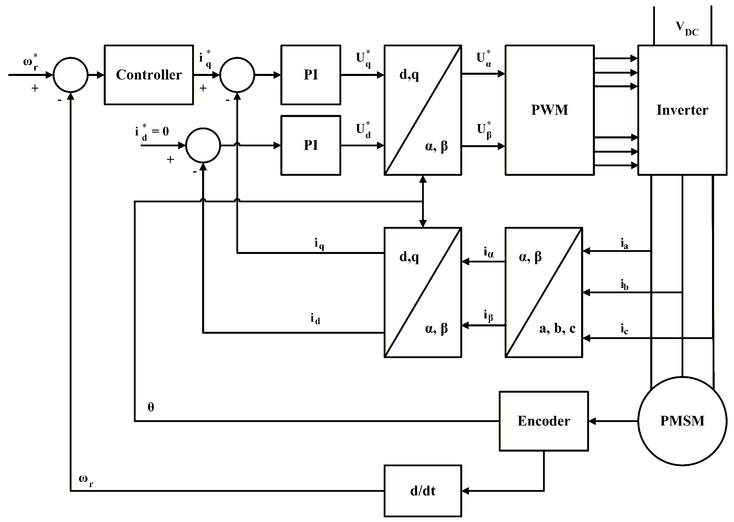
Field-Oriented Control (FOC) [20] is a widely used technique for controlling permanent magnet synchronous motors similar to the principle of DC motors: by using the park transformation to transform the three phases into the d-q axis, this method divides the control loop into two parts, where the first is the current loop and the second is the speed loop. The control structure is shown in Figure 1 [21].

To model the permanent magnet synchronous motor, the following assumptions must be applied [22]. Iron core saturation, eddy currents, and hysteresis losses are neglected; the induced EMF is sinusoidal, and there are no field current dynamics. Utilizing the rotating rotor reference frame d-q, the mathematical model of the permanent magnet synchronous motor can be expressed using the following Equations (1) and (2) [23].

$$V_d=R_s{i}_d-{\omega }_r{\lambda }_q+\rho {\lambda }_d$$

(1)

$$V_q=R_s{i}_q-{\omega }_r{\lambda }_d+\rho {\lambda }_q$$

(2)

where $V_q$ is the q-axis voltage, $V_d$ is the d-axis voltage, $I_q$ is the q-axis current, $I_d$ is the d-axis current, $R_s$ is the stator resistance, $L_q$ is the q-axis inductance, $L_d$ is the d-axis inductance, ${\lambda }_f$ is the linkage flux.

The electromagnetics torque is represented by the following Equation (3) [24].

$$T_e={\displaystyle \frac{3}{2}}\left({\displaystyle \frac{P}{2}}\right)i_q{i}_d(L_d-L_q)+{\lambda }_f.$$

(3)

where $T_e$ is the electric torque and P is the number of poles.

The motor dynamics are represented by Equation (4) [25].

$$T_e=T_L+B{\omega }_m+J{\displaystyle \frac{d{\omega }_m}{dt}}$$

(4)

where $T_L$ denotes the torque load, B denotes the viscous friction coefficient, J denotes the moment of inertia and ${\omega }_m$ denotes the angular speed.

The FOC method approaches the constant torque by setting the $i_d$ reference to 0, which decouples the torque and flux component; electromagnetics torque can be simplified to the following Equation (5) [26].

$$T_e={\displaystyle \frac{3}{2}}\left({\displaystyle \frac{P}{2}}\right){\lambda }_f{i}_q$$

(5)

where $K_t$ is the torque constant

Therefore, the speed and torque are controlled by controlling the $i_q$ reference which gives the motor dynamic equations as the following Equations (6) and (7) [27].

$${\displaystyle \frac{d{\omega }_m}{dt}}={\displaystyle \frac{1}{J}}(T_e-T_L-B{\omega }_m)$$

(6)

$${\displaystyle \frac{d{\omega }_m}{dt}}={\displaystyle \frac{1}{J}}(k_t{i}_q-T_L-B{\omega }_m)$$

(7)

The simulation can also be configured using the data presented in

Table 1. Specifications of permanent magnet synchronous motor.

Parameter	Value
Pole pairs (P)	4
d-axis stator inductance ($L_d$)	0.42 mH
q-axis stator inductance ($L_q$)	0.57 mH
Stator resistance ($R_s$)	0.028 $\mathsf{\Omega }$
Flux linkage (${\lambda }_f$)	0.23 Wb
Moment of inertia (J)	0.02 kg m2
Viscous friction coefficient ($B_v$)	0.004 Nms

.

3. Sliding Mode Control

The concept of sliding mode control (SMC) emerged in the late 1950s through the work of V. I. Utkin and S. V. Emelyanov, who developed it as part of early research on variable-structure control systems [28]. Sliding mode control has advantages in disturbance rejection and parameter uncertainty meaning it is a robustness control method [29], but the challenge of its design is the chattering phenomenon caused by high-frequency switching which can result in damage to the sensitive device [30]. The main design consists of three parts: designing the sliding surface, reaching laws selection and obtaining the control law [31].

A sliding surface is a plane system that desires behavior of the system. This study focuses on tracking the speed error; therefore, the conventional sliding surface is represented in the following Equation (8) [32].

$$s\left(t\right)=ce\left(t\right)+\dot{e}; c>0$$

(8)

where $e\left(t\right)$ is the error and c are variables that impact convergence rate.

The error and its derivative are defined by the following Equations (9) and (10) [33].

$$e\left(t\right)={\omega }_r^{*}-{\omega }_r$$

(9)

$$\dot{e}\left(t\right)={\dot{{\omega }_r}}^{*}-\dot{{\omega }_r}$$

(10)

where ${\omega }_r^{*}$ is the speed reference and its derivative ${\omega }_r$ is the actual speed of the motor.

Chattering reduction can be achieved by several methods [34]. The reaching law method is applied in this study, and the constant rate reaching law is applied, as expressed in Equation (11) [35].

$$\dot{s}=-ϵ·sgn\left(s\right); ϵ>0$$

(11)

where $ϵ$ is a constant variable.

Furthermore, reducing chattering in the the boundary layer method is implemented by replacing the sign function with the saturation function, defined as the following Equation (12) [36].

$$sat\left(s\right)=\left\{\begin{array}{cc}1\hfill & s>\delta \hfill \\ ks\hfill & \left|s\right|\le \delta ;k={\displaystyle \frac{1}{\delta }}\hfill \\ -1\hfill & s<-\delta \hfill \end{array}\right.$$

(12)

The equivalent control is obtained from the state variable and the sliding surface and is expressed as Equation (13).

$$i_{eq}={\displaystyle \frac{1}{K_t}}[JC({\omega }_{ref}-{\omega }_r)+B{\omega }_r+T_L]$$

(13)

By integrating the equivalent and switching control actions, the resulting control law can be defined as Equation (14):

$$i_{eq}={\displaystyle \frac{1}{K_t}}[JC({\omega }_{ref}-{\omega }_r)+B{\omega }_r+T_L+Jϵsat\left(s\right)]$$

(14)

Stability Analysis

The stability of the proposed sliding mode controller was demonstrated using Lyapunov-based analysis [37], ensuring that the system trajectories converge to a bounded region around the sliding surface, determined by the boundary layer thickness $\delta$. The Lyapunov function is defined as Equation (15) [33,34,35,36].

$$V\left(s\right)={\displaystyle \frac{1}{2}}{s}^2$$

(15)

And its derivative is defined as Equation (16):

$$\dot{V}=s\dot{s}$$

(16)

Substituting the control law yields Equation (17):

$$\dot{V}=s·(-ϵ·sat\left(s\right))$$

(17)

This is always non-positive, indicating that the system is Lyapunov-stable and the error is limited to the boundary layer of size $\delta$. The Chess Optimization Algorithm does not remove this bound, but minimizes its practical size: because the ITAE/ITSE objective is weight tracking error by elapsed time, persistent steady-state error is penalized heavily, driving COA toward the smallest feasible $\delta$ paired with a switching gain $ϵ$ that keeps the error near the inner edge of the boundary layer without reintroducing chattering. 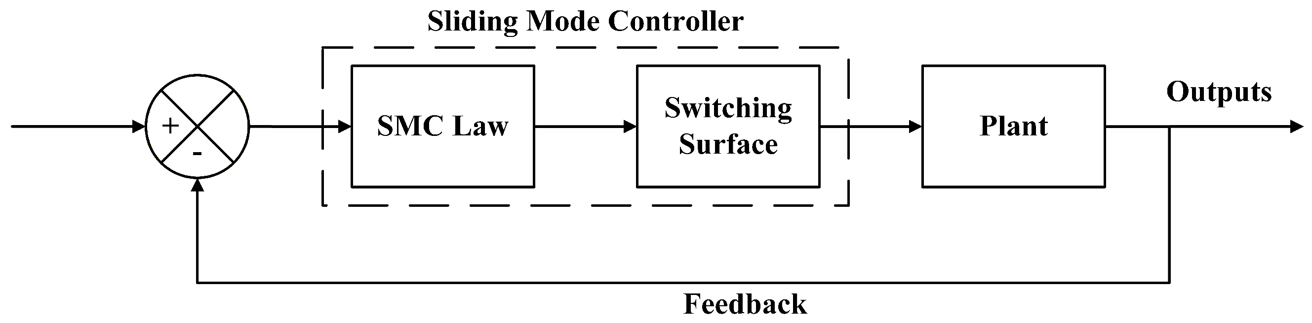Figure 2 shows a diagram illustrating the sliding mode controller.

4. Chess Optimization Algorithm

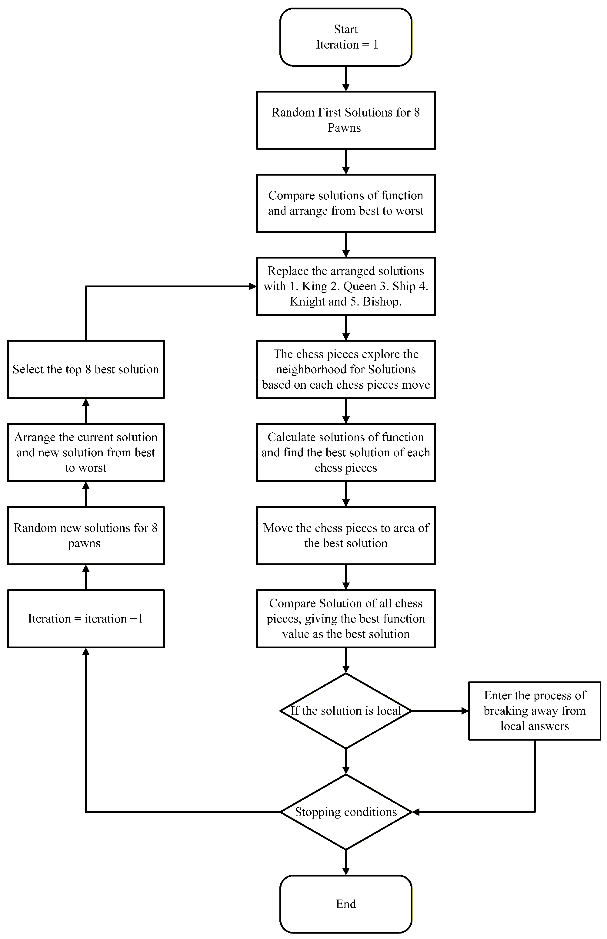
The principles and strategies of international chess games are the inspiration for the optimization algorithm. The specific movement of each chess piece creates a method for determining the optimal value for the problem. The promotion of pawn pieces into higher chess pieces such as queen, king, bishop, rook, and knight is also involved in the algorithm creating a new strategy and escaping the local value. The operation of the Chess Optimization Algorithm is shown in Figure 3.

1:

Generate an initial population by randomly placing eight pawns within the defined constraints to create diverse candidate solutions.

2:

Evaluate each pawn configuration using the objective function and identify the most promising candidates.

3:

Form the second group of pieces, namely one king, one queen, two rooks, two knights, and two bishops, to represent structured strategic moves.

4:

Each piece is assigned individually to understand its influence on improving the current solution.

5:

Conduct a local search for each setup and identify optimal neighboring alternatives.

6:

Rearrange components to augment their efficacy and refine the overall search trajectory.

7:

Compare all search solutions and record the solution that exhibits the highest performance for the present iteration.

8:

Examine global conditions and optimize the search to prevent becoming ensnared in a local solution.

9:

Check the stopping condition. If they are not satisfied, add the iteration count and continue.

10:

Randomize the eight new pawns to create variety and start the procedure anew.

11:

Align the optimal principal pieces with the pawn, compare all 16 solutions and sort them from best to worst.

12:

Focus on the eight leading answers and repeat the enhancement procedure until the termination condition is satisfied.

The three-dimensional solution vector for the sliding mode controller optimization is encoded as $X_p=[C,ϵ,\delta ]$, representing the sliding surface slope coefficient, the reaching switching gain, and the saturation boundary layer thickness, respectively. Algorithm 1 presents the pseudocode with position update for each chess pieces. Each of these roles—king, queen, rook, bishop, and knight—is given a particular movement weight that dictates the size of their steps and their capacity for exploration. While the king and queen display more expansive dynamic behaviors to allow for extended exploration of the search space, the rook, bishop, and knight follow directed or local movement patterns for precision changes.

Algorithm 1 Chess Optimization Algorithm (COA)

1: procedure Initialize($N_p,[LB,UB],X_p$)   2:     for $i=1,\dots ,N_p$ do   3:         ${\mathbf{x}}_i\sim \mathcal{U}(LB,UB)$   4:     end for   5:     $iteration\leftarrow 0$   6: end procedure   7: procedure Optimize   8:     while $iter<I_{max}$ do   9:         evaluate fitness $f\left({\mathbf{x}}_i\right)$ for all pawns 10:         find neighborhood and select best neighborhood 11:         for $i=1,\dots ,N_p$ do 12:            $queen\_w=[0.01,0.03,0.05,0.10,0.20,0.50,1.00,1.50]$ 13:            $king\_w=[0.0125,0.0150,0.0175,0.019,0.02,0.025,0.0275,0.03]$ 14:            $rooks\_w=[0.1,0.2,0.35,0.5,0.6,0.7,0.9,1.0]$ 15:            $bishops\_w=[0.125,0.225,0.375,0.525,0.625,0.725,0.925,1.25]$ 16:            $knight\_w=[0.11,0.12,0.13,0.14,0.20,0.21,0.22,0.23]$ 17:            $N\_UB\leftarrow X_p+P_w$ and $N\_LB\leftarrow X_p-P_w$ 18:            if $N\_UB\ge UB$ then 19:                $N\_UB\leftarrow UB$ 20:            else if $N\_LB\le LB$ then 21:                $N\_LB\leftarrow LB$ 22:            end if 23:            $X_p\leftarrow N\_LB+rand\left(\right)·(N\_UB-N\_LB)$ 24:         end for 25:         Evaluate fitness & rank candidate moves; select the best solution 26:         assign $N_p$ pawns to generate new solutions 27:         $iteration\leftarrow iteration+1$ 28:     end while 29:     return best solution $\widehat{\mathbf{x}}$ 30: end procedure

5. Objective Function

The sliding mode parameters were optimized by optimization algorithms via two objective functions, the first being the Integral of Time-weighted Absolute Error (ITAE), as expressed in Equation (18), which emphasizes the error over time, which also makes the response of the system faster and results in less error over time [38].

$$\mathrm{ITAE}={\int }_0^{T}t·\left|e\left(t\right)\right| dt$$

(18)

Secondly, the Integral of Time-weighted Square Error (ITSE), as expressed in Equation (19), penalizes the large error, which makes the response of the system less oscillating [39].

$$\mathrm{ITSE}={\int }_0^{T}t·e{\left(t\right)}^2 dt$$

(19)

6. Mean Absolute Error and Root Mean Square Error

6.1. Mean Absolute Error (MAE)

The Mean Absolute Error (MAE) characterizes the average absolute difference between the commanded and measured motor speeds. This is expressed in Equation (20) [40]:

$$\mathrm{MAE}={\displaystyle \frac{1}{N}}{\displaystyle \sum _{k=1}^N}|{\omega }_{ref}\left(k\right)-{\omega }_r\left(k\right)|$$

(20)

MAE offers a definitive measure of the controller’s comprehensive tracking precision. The reduced MAE values signify that the controller sustains the specified speed with greater consistency, facilitating the assessment of the steady-state accuracy and overall tracking efficacy.

6.2. Root Mean Square Error (RMSE)

The Root Mean Square Error (RMSE) characterizes the magnitude of the tracking deviations and emphasizes larger errors owing to its squared formulation. This is expressed in Equation (21) [40]:

$$\mathrm{RMSE}=\sqrt{{\displaystyle \frac{1}{N}}\sum _{k=1}^N{({\omega }_{ref}\left(k\right)-{\omega }_r\left(k\right))}^2}$$

(21)

The RMSE is very useful for detecting oscillatory patterns and sensitivity to disturbances. A reduced RMSE signifies more consistent responses with fewer significant deviations and serves as a robust indicator of controller resilience in dynamic situations.

7. Simulation Result

The speed control of the permanent magnet synchronous motor and controller was simulated using MATLAB/Simulink R2021a. All simulations were executed on a laptop. The simulation parameters are employed using a variable-step ODE45 solver, and the maximum number of iterations for all optimization algorithms was set to 100. It should be noted that the comparative paths and performance indexes tested among COA, HHO and WOA are from single representative optimization runs under the same conditions. Thus, these metrics represent specific deterministic performance profiles, not general statistical superiority over multi-trial stochastic distributions. During the execution of optimization, the parameters’ ranges are as follows: $0<C<3000$; $0<ϵ<1\times {10}^6$; $0<\delta <1.5$.

The results are compared in two main sections: optimization algorithms and controller performance. All comparisons encompassed three testing scenarios. The initial scenario validates the speed response to analyze the time-domain performance. The second scenario evaluates the ability of the system to handle speed variations, validating its robustness against parameter changes. The final scenario applies a load disturbance to analyze how well the system rejects disturbances. The optimal sliding mode controller parameters obtained using ITAE and ITSE as objective functions are listed in

Table 2. Sliding mode controller’s parameter setting using ITAE as objective function.

Optimization Algorithm	Tuned Parameters
	c	$\epsilon$	$\delta$
COA	1779.5796	521,240	0.6765
HHO	1793.3457	811,504	0.4263
WOA	1789.3568	303,830	1.1527

and

Table 3. Sliding mode controller’s parameter setting using ITSE as objective function.

Optimization Algorithm	Tuned Parameters
	c	$\epsilon$	$\delta$
COA	1913.0651	818,800	1.4380
HHO	1911.4422	572,964	0.5952
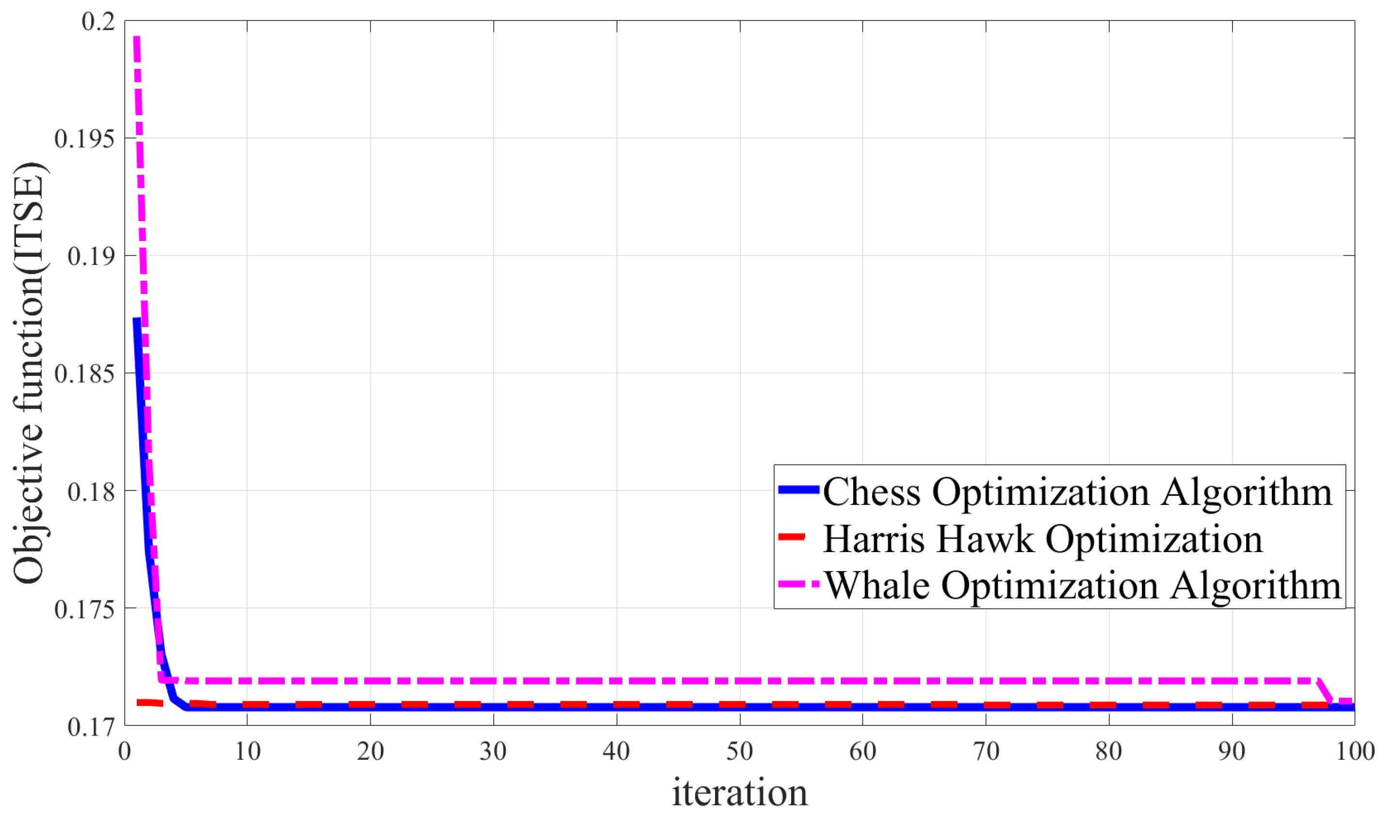
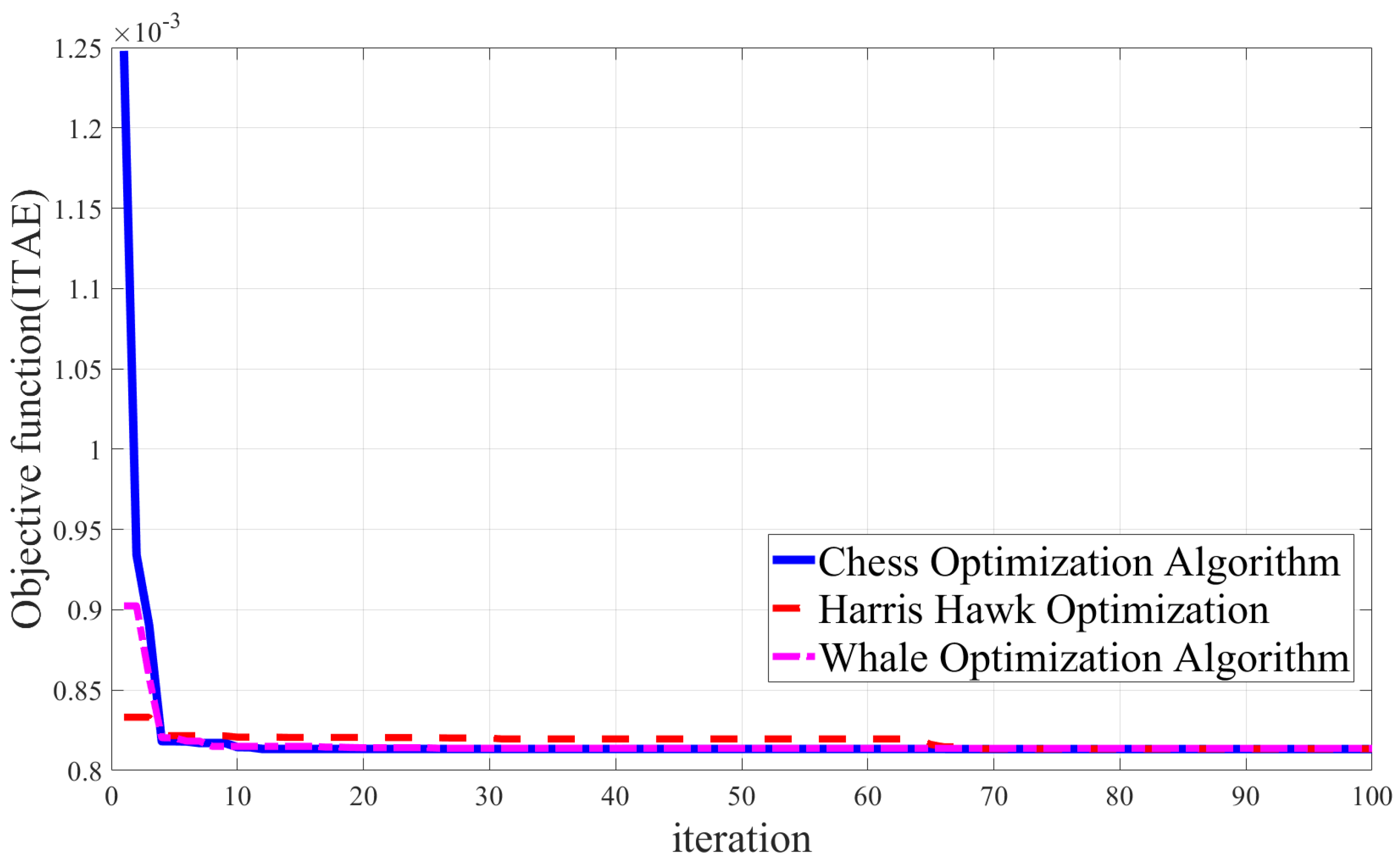
WOA	2001.2709	513,504	1.4600

. The convergence curves of ITAE and ITSE are shown in Figure 4 and Figure 5, respectively.

The selection of Harris Hawks Optimization (HHO) and the Whale Optimization Algorithm (WOA) as comparative baselines is directly motivated by recent developments in the electrical drive-tuning literature. HHO and WOA represent a prominent, highly competitive generation of modern swarm intelligence that utilizes fundamentally distinct mathematical exploration models—specifically cooperative aerial hunting and marine bubble-net spiral updates.

In some cases, the optimal switching gain $ϵ$ takes on very large values for all three algorithms, such as 818,800 for COA under ITSE (Table 3) and 811,504 for HHO under ITAE (Table 2), indicating that this is due to the interaction of the objective functions with the control law, not a peculiarity of COA’s search behavior specifically. Since $\mathrm{sat}\left(s\right)$ in (14) is limited to $[-1,1]$ for any value of $ϵ$, the correction term $J·ϵ·\mathrm{sat}\left(s\right)$ is limited to $\pm J·ϵ$, so a greater $ϵ$ reinforces the restoring effect without causing the output to exceed the bounded limits, which is why all three algorithms tend to converge for large $ϵ$ to reduce the time-weighted ITAE/ITSE error. However, the absolute value $J·ϵ$ should be checked against the actual current and voltage ratings of the drive, as this product determines the real control effort required from the inverter. A necessary improvement prior to physical realization is to restrict the search bounds of $ϵ$ accordingly.

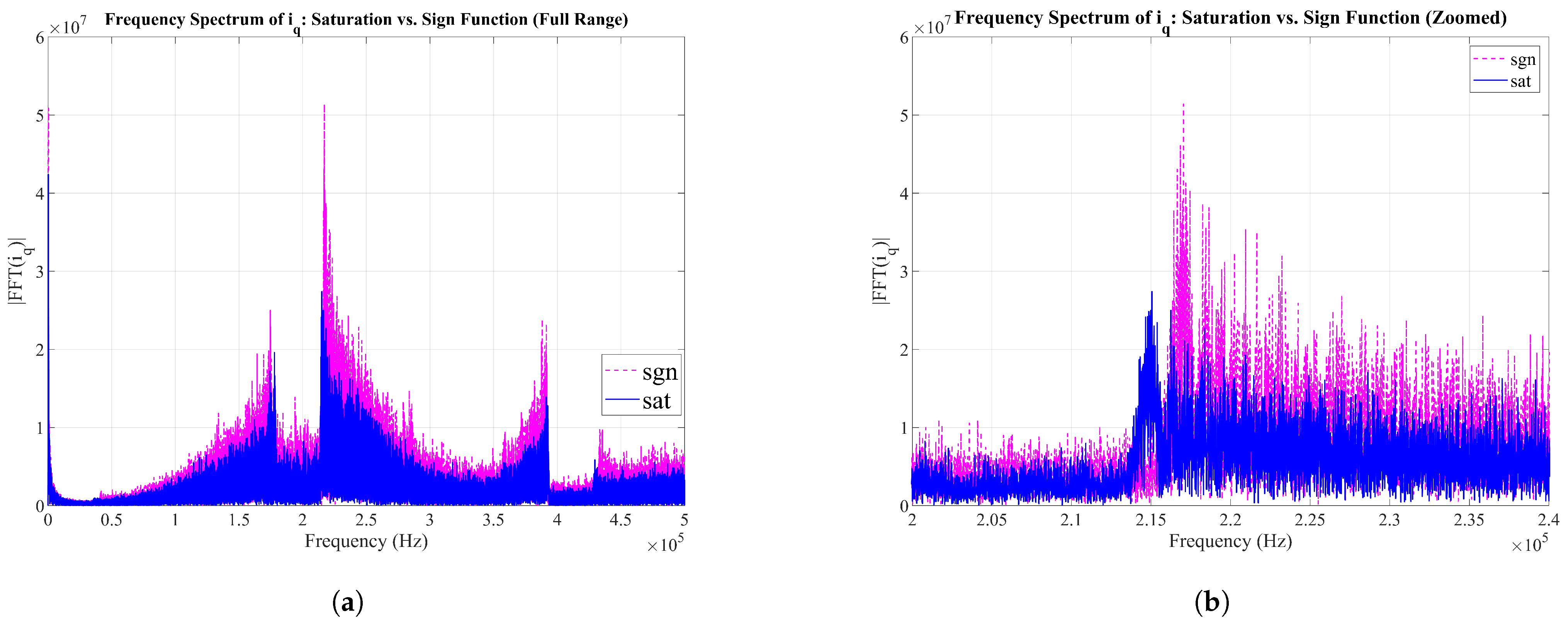
To quantify the chattering reduction due to the saturation function, the steady-state q-axis current was evaluated using four time-domain metrics and one spectral metric, comparing the saturation-function-based controller with the sign-function-based controller under the same parameters.

Table 4. Quantitative chattering comparison: saturation function vs. sign function.

Metric	sgn	sat	Reduction (%)
Standard deviation	14,671.2683	9918.1227	32.40
Total variation	1,103,760,336.3752	743,178,012.8783	32.67
Peak-to-peak ripple	30,217.4935	20,441.2609	32.35
High-frequency RMS	14,712.6344	9939.2036	32.44
High-frequency spectral energy ($f>1 \mathrm{kHz}$)	$1.0529\times {10}^{18}$	$4.8252\times {10}^{17}$	54.17

shows that the saturation function reduced the standard deviation of the steady state current by 32.40%, the total variation by 32.67%, the peak-to-peak ripple by 32.35%, and the high frequency RMS component by 32.44% when compared to the sign function.

These four metrics agree closely, indicating that the reduction in chattering amplitude is consistent across several measures of the chattering amplitude, and not an artifact of any one measure. This result is verified by the spectral comparison in Figure 6. The spectral comparison of sign-function to saturation-function is about two times at the dominant peak around 217 kHz and the high-frequency spectral energy above 1 kHz is reduced by 54.17% with the saturation function. Together these results provide a visual and quantitative confirmation that the boundary-layer saturation function provides significant suppression of high frequency switching content compared to the discontinuous sign function, as expected for its purpose of mitigating chattering.

7.1. The Comparison of the Different Algorithm Using ITAE as Objective Function

7.1.1. Speed Response

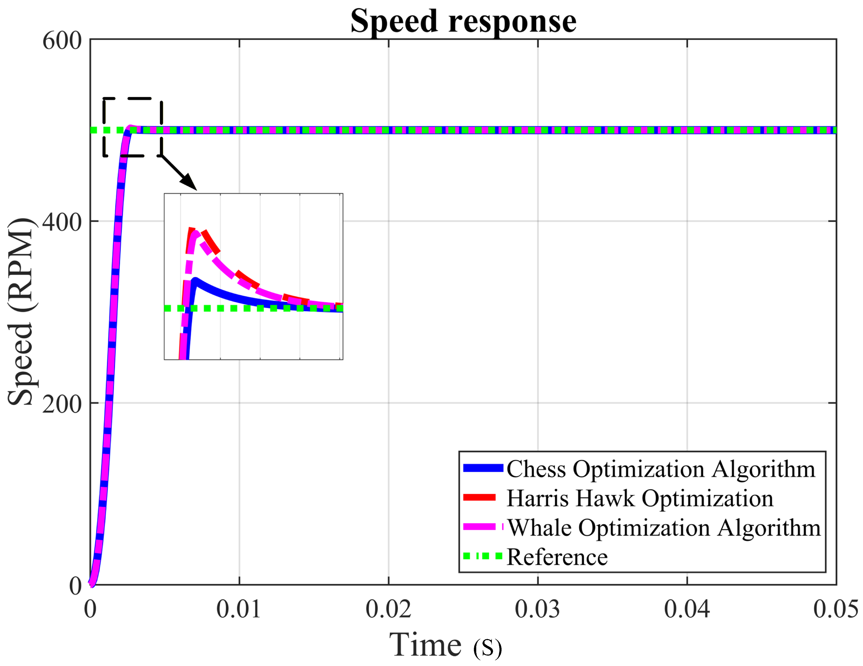
Figure 7 presents the transient behavior of the system, and

Table 5. Time-domain response using ITAE as objective function.

Optimization Algorithm	Rise Time (s)	Settling Time (s)	Overshoot (%)	ITAE
COA	0.001494	0.002421	0.1929	0.0008133
HHO	0.001488	0.002402	0.6164	0.0008135
WOA	0.001489	0.002407	0.5103	0.0008138

provides numerical details that compare the performance of each optimization method. The COA achieved the best performance, with the lowest overshoot and ITAE at 0.1929% and 0.0008133, respectively. However, it also had poor performance in terms of rise time at 0.001494 s and settling time at 0.002421 s. This shows that COA gives the system a smoother and more stable reaction. In contrast, the HHO gave the best performance in rise time and settling time at 0.001488 s and 0.002402 s, respectively. Although it obtained the fastest response time for the system, it also had the largest overshoot, suggesting that it may affect the system’s stability during the initial phase.

The WOA obtained decent performance, with slightly slower rise time and settling time than the HHO at 0.001489 s and 0.002407 s, respectively. The second largest overshoot was at 0.5103%. In terms of ITAE, the WOA obtained the largest ITAE at 0.0008138. This shows that even with the decent performance, it still achieved the largest error. These results suggest that COA provides a more balanced optimization by emphasizing stability and reduced tracking error, whereas HHO and WOA make fast response over the error stabilized with high overshoot.

7.1.2. Speed Change Response

In this scenario, the parameter variation is analyzed by altering the reference speed to assess the resilience of each method under varying operating conditions. The mean absolute error (MAE) and the root mean square error (RMSE) were used to measure robustness.

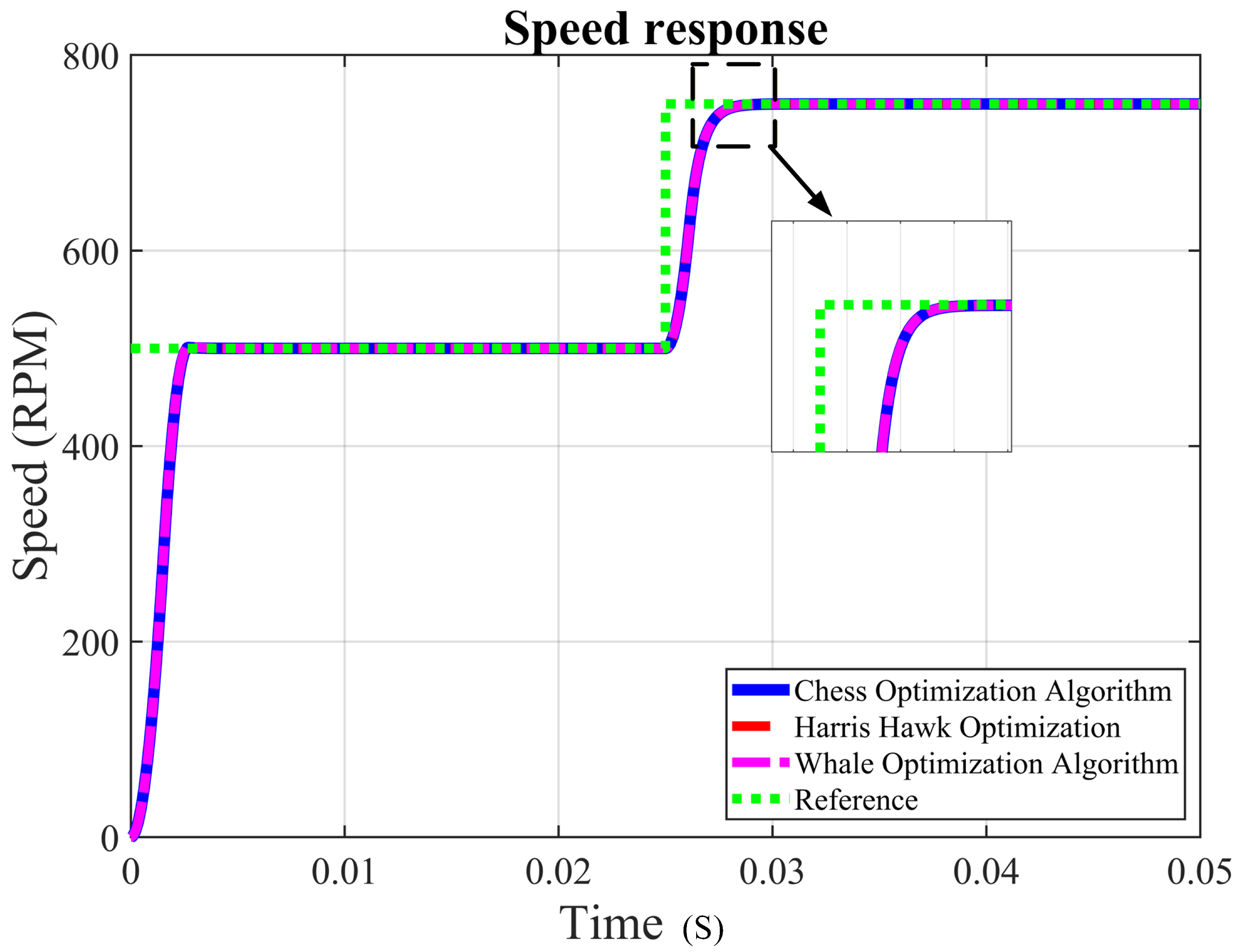
Figure 8 shows that when the input speed is raised to 750 rpm, the error tracking after the change of input speed seems to give similar performance. However, the HHO give the most accuracy due to the lowest MAE and RMSE at 20.0046 and 80.3589, respectively. The COA obtained the second best error tracking with the value of MAE at 20.0119 and RMSE at 80.3776; the WOA, on the other hand, records the largest value of MAE at 20.163 and RMSE at 80.3790.

The statistical error metrics, shown in

Table 6. Comparison of MAE and RMSE for different algorithms in speed change response.

Optimization Algorithm	MAE	RMSE
COA	20.0119	80.3776
HHO	20.0046	80.3589
WOA	20.0163	80.3790

, show that the HHO-tuned parameters demonstrate strong robustness against the change of parameters. The COA-tuned parameters achieved moderate error tracking, showing slightly larger deviations than HHO. Meanwhile, the WOA-tuned parameters exhibit comparable behavior but produce slightly higher error and greater deviation.

7.1.3. Load Response

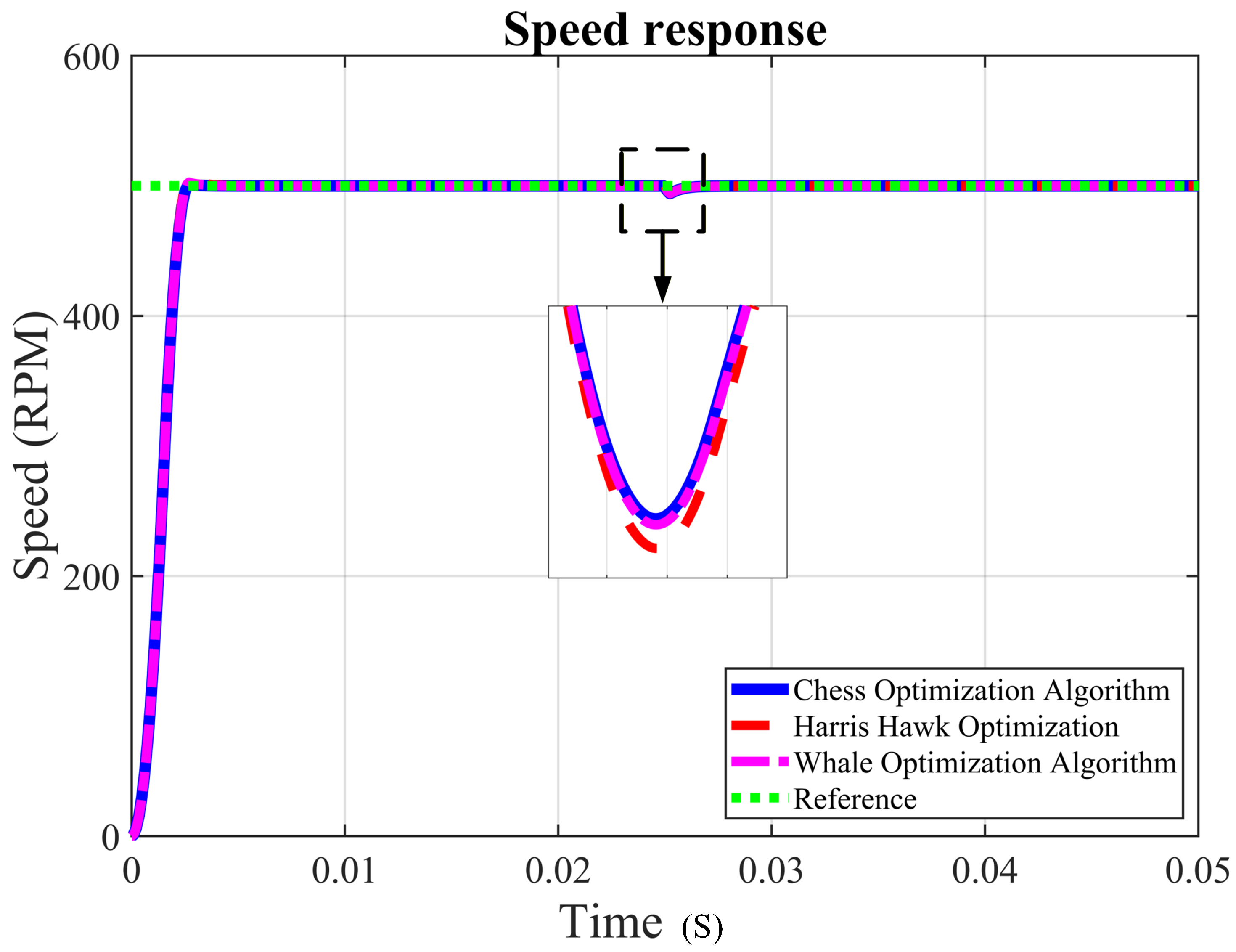
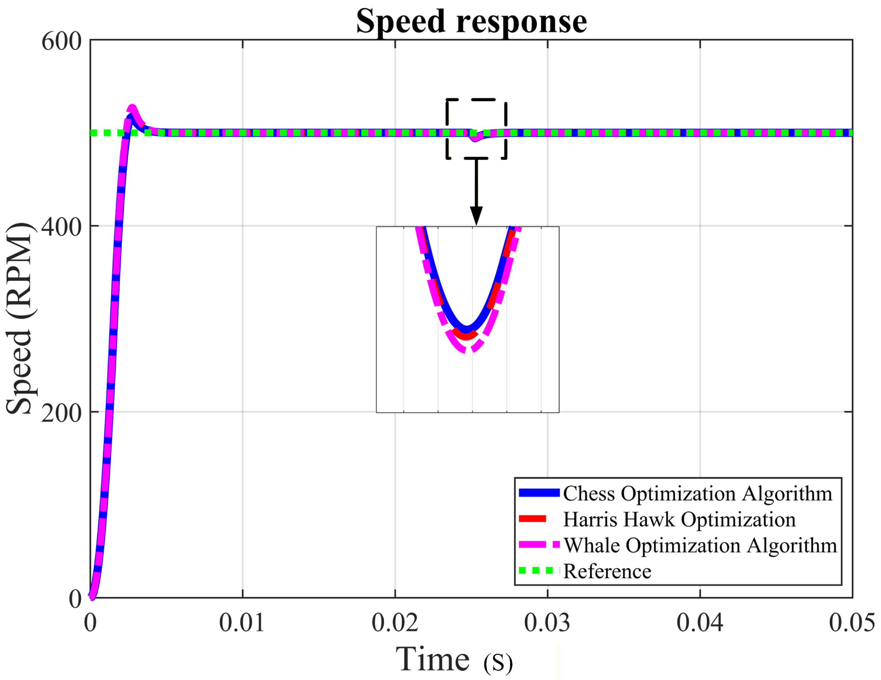
The third case examined how well the system could reject disturbances when a load was applied at 0.025 s. The mean absolute error (MAE) and root mean square error (RMSE) were used to measure the extent to which a system can handle disturbances. The COA showed the smallest speed drop, that being only 0.3039%, as shown in Figure 9.

Figure 9 shows that the COA had the smallest deviation from the reference speed after the load disturbance. Meanwhile, the WOA is inbetween the COA and HHO, indicating that the disturbance rejection is decent. In contrast, the HHO had the largest drop of speed, which shows that it had comparatively weaker disturbance rejection.

Table 7. Comparison of MAE and RMSE for different algorithms under load conditions.

Optimization Algorithm	MAE	RMSE
COA	14.0409	73.2964
HHO	14.0649	73.2733
WOA	14.0462	73.2872

shows that the COA achieved the lowest MAE at 14.0409 but in terms of RMSE, the COA demonstrated the largest value at 73.2964, indicating the most accurate average tracking of the reference speed. However, it comes with a moderate amount of fluctuation. The HHO, on the other hand, had the lowest RMSE at 73.2733 meaning that its behavior is less oscillating than the other, but it had the highest MAE at 14.0649, reflecting lower tracking accuracy. Meanwhile, the WOA achieved the second highest MAE at 14.0462 and RMSE at 73.2872, which indicates moderate tracking accuracy and stability.

7.2. The Comparison of the Different Algorithms Using ITSE as Objective Function

7.2.1. Speed Response

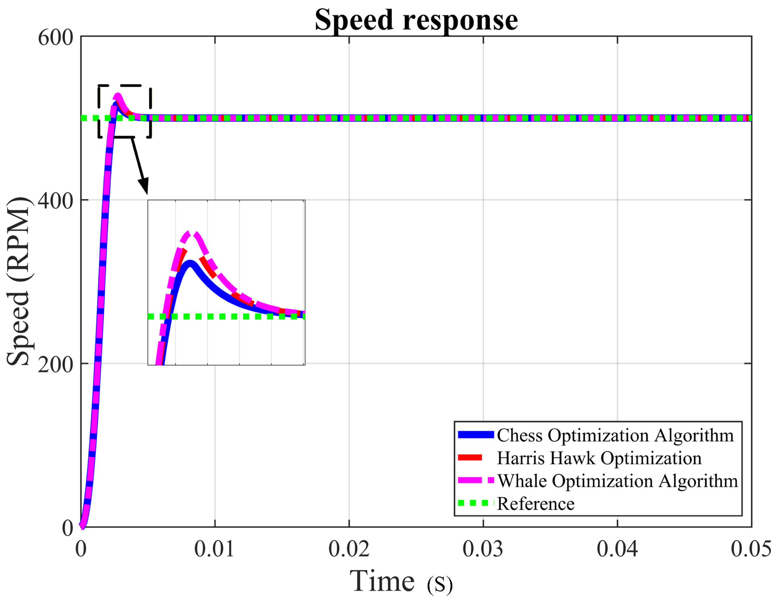
Figure 10 shows how well the controllers perform the transient response, and

Table 8. Time-domain response using ITSE as objective function.

Optimization Algorithm	Rise Time (s)	Settling Time (s)	Overshoot (%)	ITSE
COA	0.0014528	0.00307	3.4800	0.1708
HHO	0.0014333	0.00335	5.4036	0.1709
WOA	0.0014325	0.00334	5.5019	0.1711

provides more information about the numbers. The COA achieved the best performance in settling time overshoot and ITSE at 0.00307 s, 3.4800% and 0.1708, respectively. However, the COA had a disadvantage in rise time at 0.0014528 s, which indicates that the system needs a longer time to respond to the input. Meanwhile, the HHO had decent performance with balanced response in rise time, overshoot, and ITSE which are second-best to the other; it also had a longer settling time at 0.00335 s, which indicates that the response stabilizes slightly slower than COA and WOA.

The WOA only had the best performance in rise time at 0.0014325s but got poor performance in other criteria with the highest overshoot at 5.5019% and largest ITSE at 1.711, indicating that although the system is fast to respond, the system is likely to be oscillating more than others. The result shows that the COA has capability to optimize the controller to achieve smooth response, reduce overshoot, and stabilize faster compared to HHO and WOA.

7.2.2. Speed Change Response

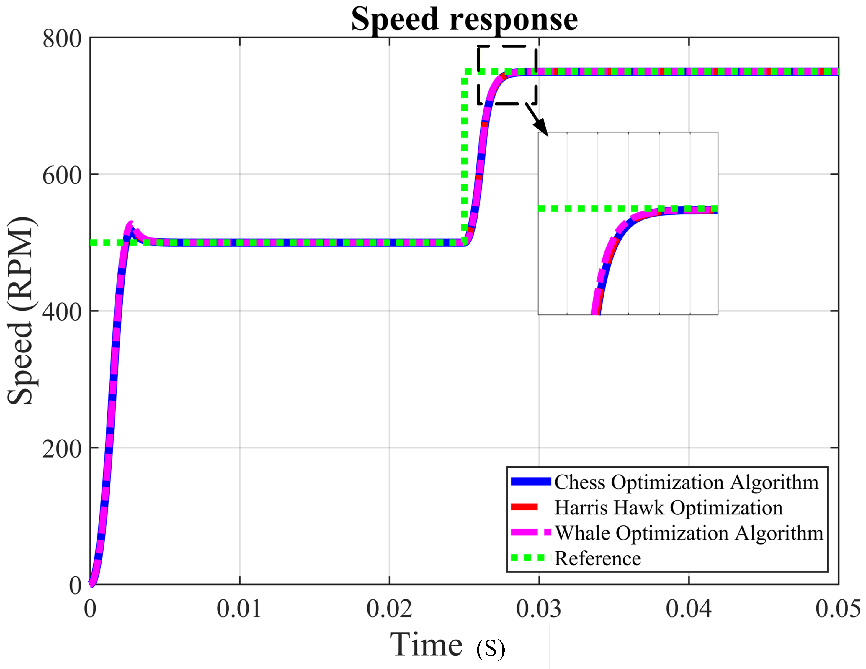
Figure 11 shows the speed response of the controllers tuned by the optimization algorithms when the input speed is changed. All controllers exhibit a similar response pattern; however, the WOA seems slightly faster than COA and HHO. The tracking performance is provided in

Table 9. Comparison of MAE and RMSE for different algorithms in speed change response.

Optimization Algorithm	MAE	RMSE
COA	20.0773	80.3305
HHO	20.1251	80.2806
WOA	20.1412	80.2885

through the MAE and RMSE metrics.

Error analysis, as shown in Table 9, provides more information about the robustness of the results. The COA achieved the lowest MAE at 20.0773, but it also had the highest RMSE at 80.3305. The HHO achieved the second best MAE at 20.1251 and the lowest RMSE at 80.2806. Finally, the WOA achieved the highest MAE at 20.1412 and second best RMSE at 80.2885. The result shows that the COA provides better performance in error tracking, but it has disadvantages in the reduced deviation of error. On the other hand, the HHO demonstrates better performance in minimizing error deviation. Meanwhile, the WOA provides decent performance with poor error tracking and less deviation compared to COA.

7.2.3. Load Response

Figure 12 shows what happens to the system when a load is applied. The COA produces the smallest speed drop among the algorithms, indicating the strongest disturbance rejection capability followed by the HHO, while the WOA has the biggest drop.

The error metrics, as shown in

Table 10. Comparison of MAE and RMSE for different algorithms under load conditions.

Optimization Algorithm	MAE	RMSE
COA	14.1709	73.2416
HHO	14.3142	73.2426
WOA	14.3079	73.2427

, further support these findings. The COA achieved the lowest MAE and RMSE, at 14.1709 and 73.2416, respectively. The HHO achieved the highest MAE at 14.3142 but it has the second lowest RMSE at 73.2426. Finally, the WOA achieved the second lowest MAE at 14.3079 and highest RMSE at 73.2427. The result shows that COA provides the best performance in error tracking and minimizing error deviation; meanwhile, HHO offers slightly poorer average tracking accuracy but relatively stable error variation. WOA also offers decent tracking with larger error deviation.

7.3. The Comparison of the Different Controllers Using ITAE as Objective Function

7.3.1. Speed Response

To establish a transparent baseline for controller performance comparisons, the classical PI and PID speed controllers were optimized using COA under identical objective criteria. The resulting optimized control loop parameters are listed in

Table 11. PI and PID controllers’ parameter settings using ITAE as objective function.

Controller	Tuned Parameters
	${\mathit{K}}_{\mathit{P}}$	${\mathit{K}}_{\mathit{I}}$	${\mathit{K}}_{\mathit{D}}$
PI	2.0326	810.2540	-
PID	163.6841	151.9681	0.6299

.

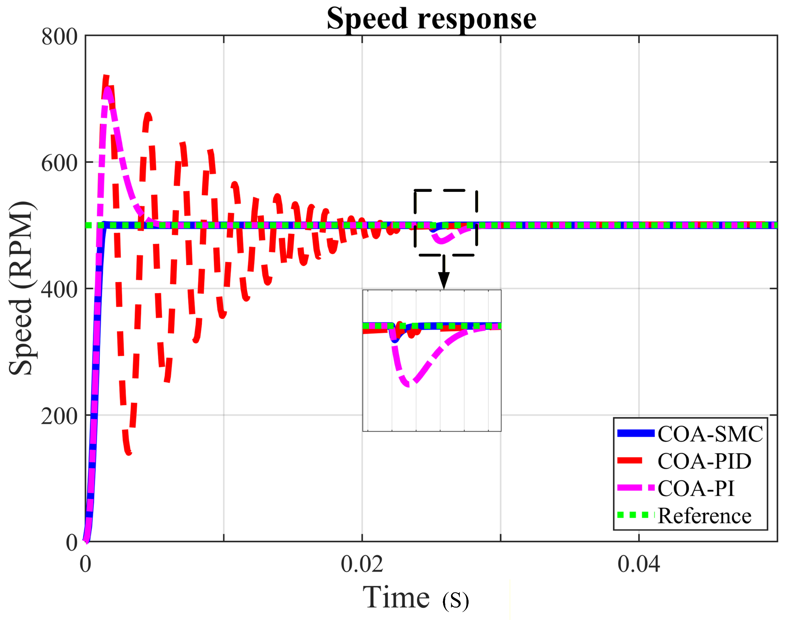
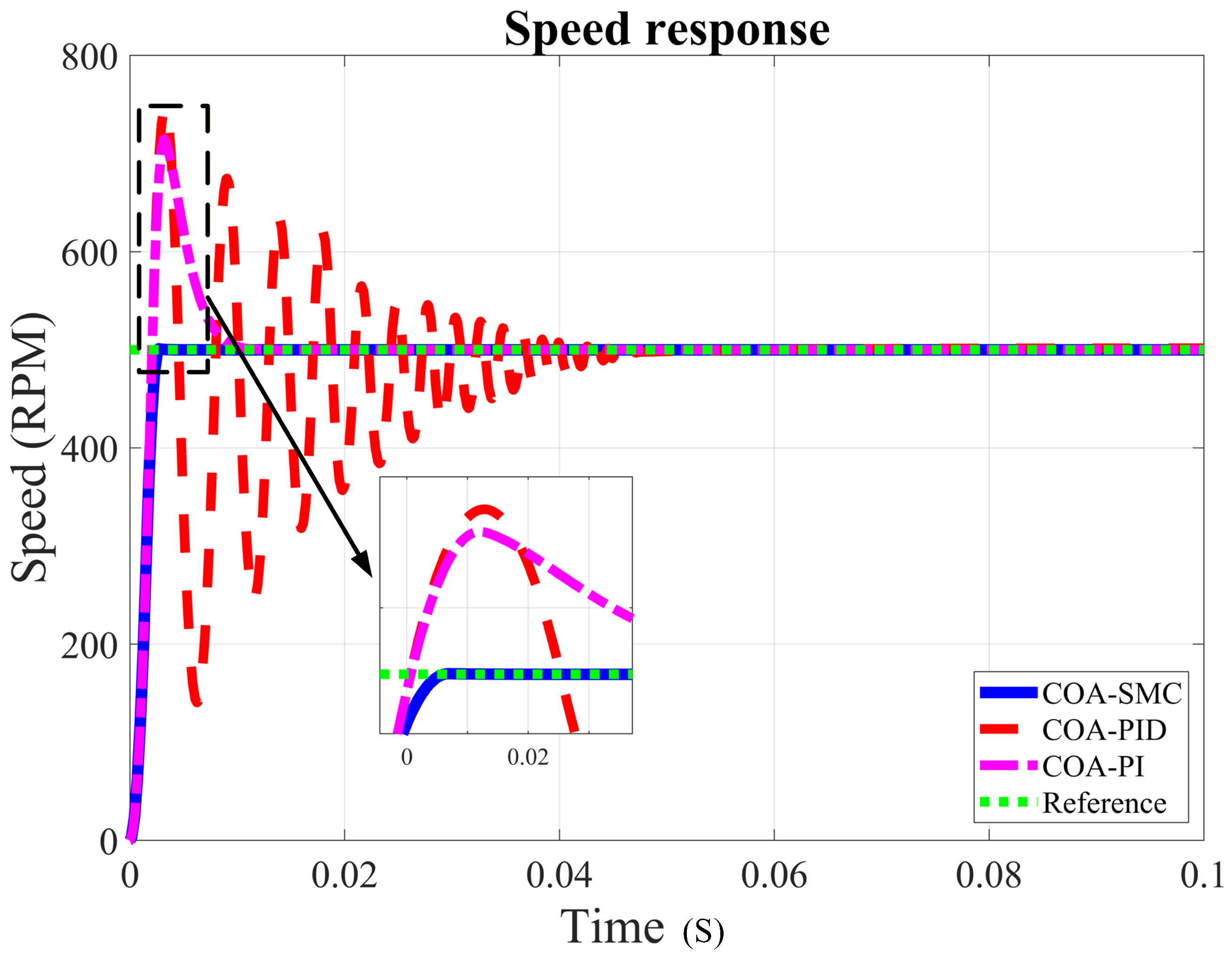
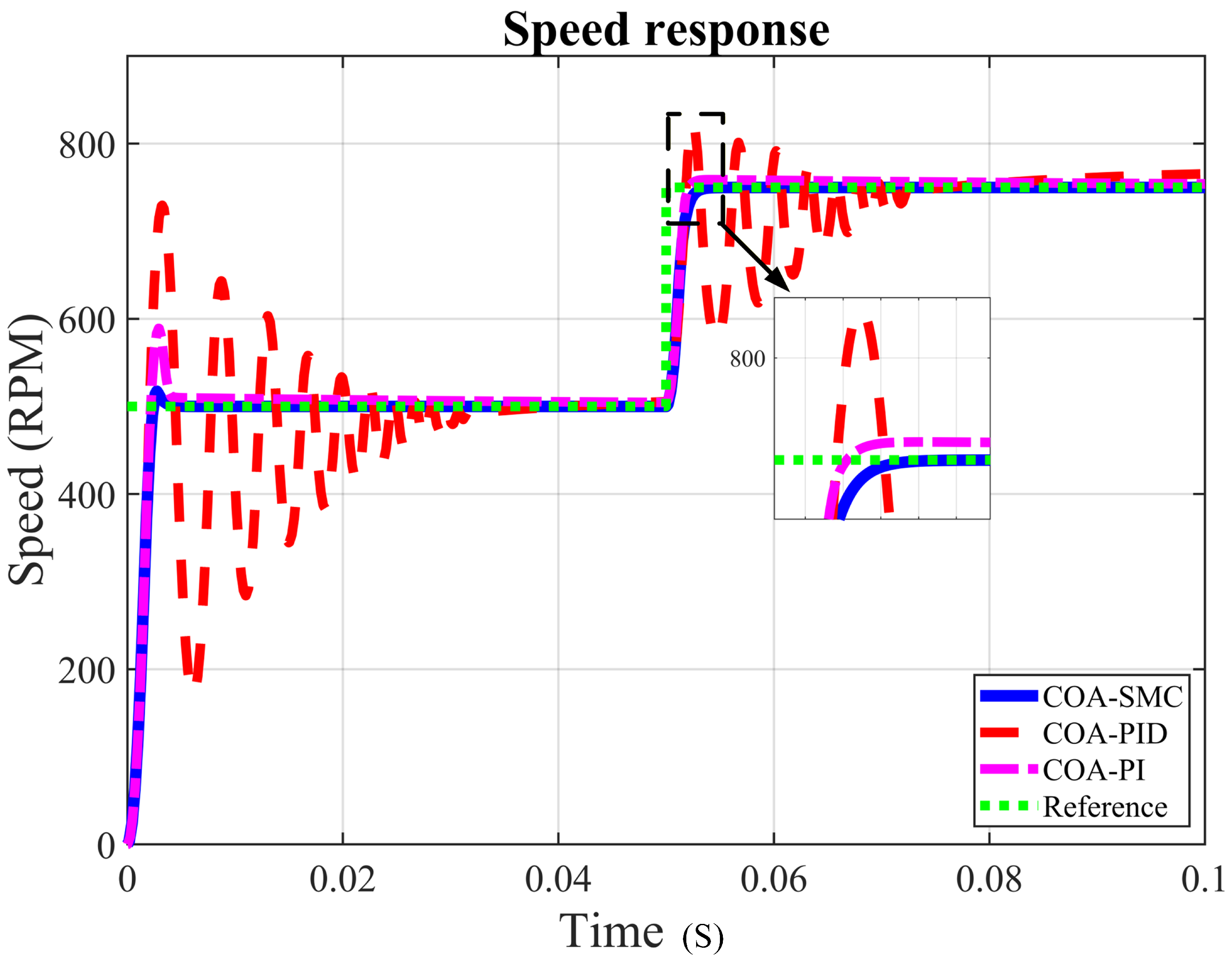
Figure 13 shows the transient response, with the additional numerical data summarized in

Table 12. Time-domain response using ITAE as objective function.

Optimization Algorithm	Rise Time (s)	Settling Time (s)	Overshoot (%)	ITAE
SMC	0.001494	0.002421	0.1927	0.0008133
PID	0.001320	0.044985	49.1591	0.0545611
PI	0.001318	0.008789	42.9117	0.0034867

. Among the controllers, the sliding mode controller provides the best overall performance, achieving the lowest ITAE value of 0.0008133. It also delivers a well-damped response with a very small overshoot of 0.1927% and a fast-settling time of 0.002421 s. However, it requires a slightly longer rise time of 0.001494 s compared to the other controllers.

The PID and PI controllers exhibit similarly fast rise times of 0.001320 s and 0.001318 s, respectively, but this comes at the cost of poorer transient behavior. The PID controller shows the largest overshoot at 49.1591% and a significantly longer settling time of 0.044985 s, indicating a highly oscillatory response. The PI controller performs moderately better yet still exhibits considerable overshoot of 42.9117% and a settling time of 0.008789 s. Overall, the sliding mode controller clearly provides the most stable and well-controlled response among the three controllers.

7.3.2. Speed Change Response

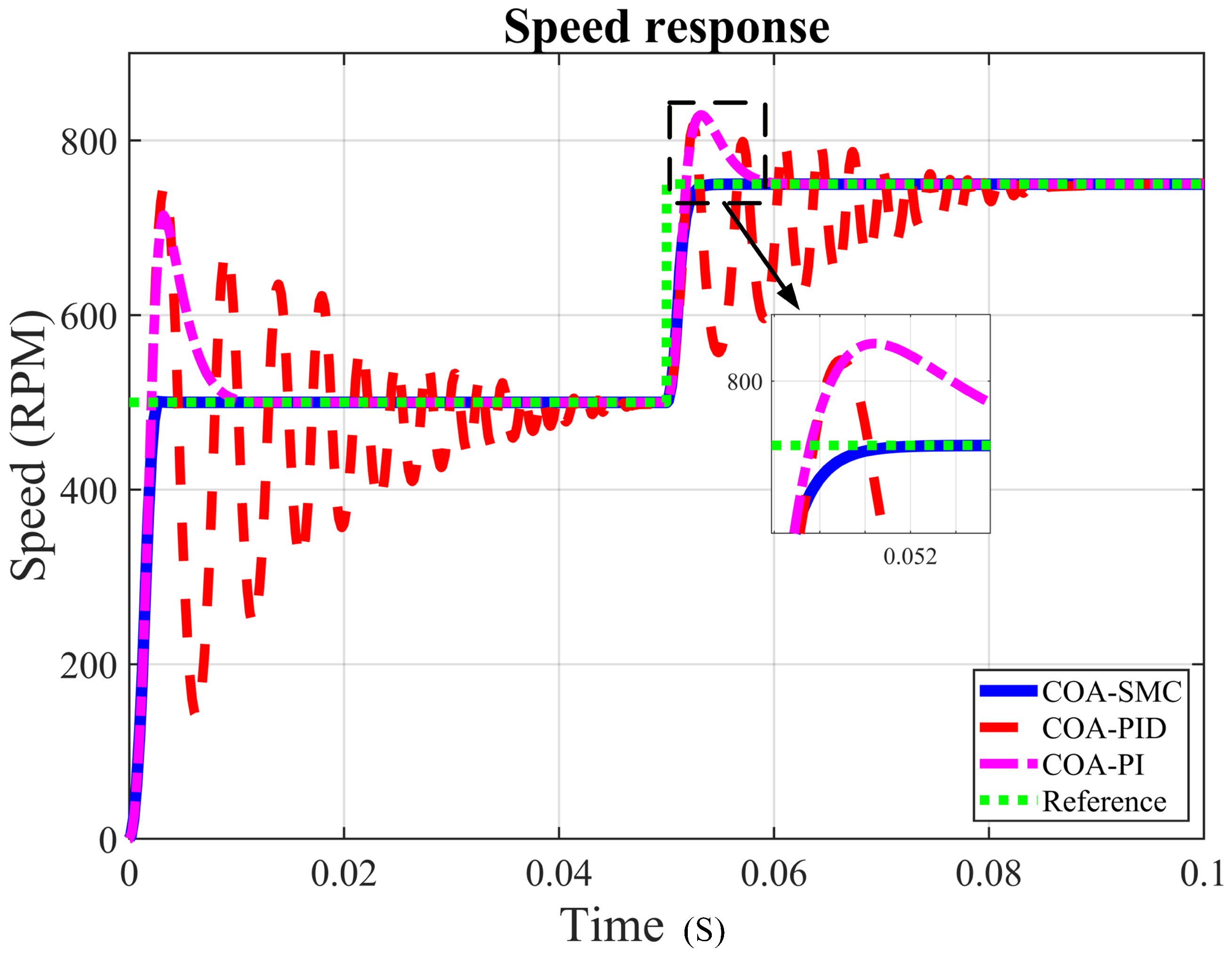
Figure 14 shows the transient response when the input speed was changed to 750 rpm at 0.05 s. The PI controller responds the fastest followed by the PID controller, while the sliding mode controller takes slightly longer. However, the sliding mode controller manages to settle faster; meanwhile, PI has a longer settling time and the PID controller has the longest settling time.

In terms of tracking accuracy,

Table 13. Comparison of MAE and RMSE for different controllers in speed change response.

Controller	MAE	RMSE
SMC	10.0307	56.8324
PID	61.2721	103.4770
PI	19.0356	65.8581

shows that the sliding mode controller achieves the lowest MAE of 10.0307 and the lowest RMSE of 56.8324, indicating that its actual speed closely follows the reference with minimal deviation. The PI controller gives the second-best performance, with an MAE of 19.0356 and an RMSE of 65.8581. The PID controller, on the other hand, has the highest MAE of 61.2721 and RMSE of 103.4770, indicating significantly larger average errors and greater deviation from the reference speed. Overall, these results demonstrate that the SMC provides superior tracking accuracy and faster stabilization under reference speed changes.

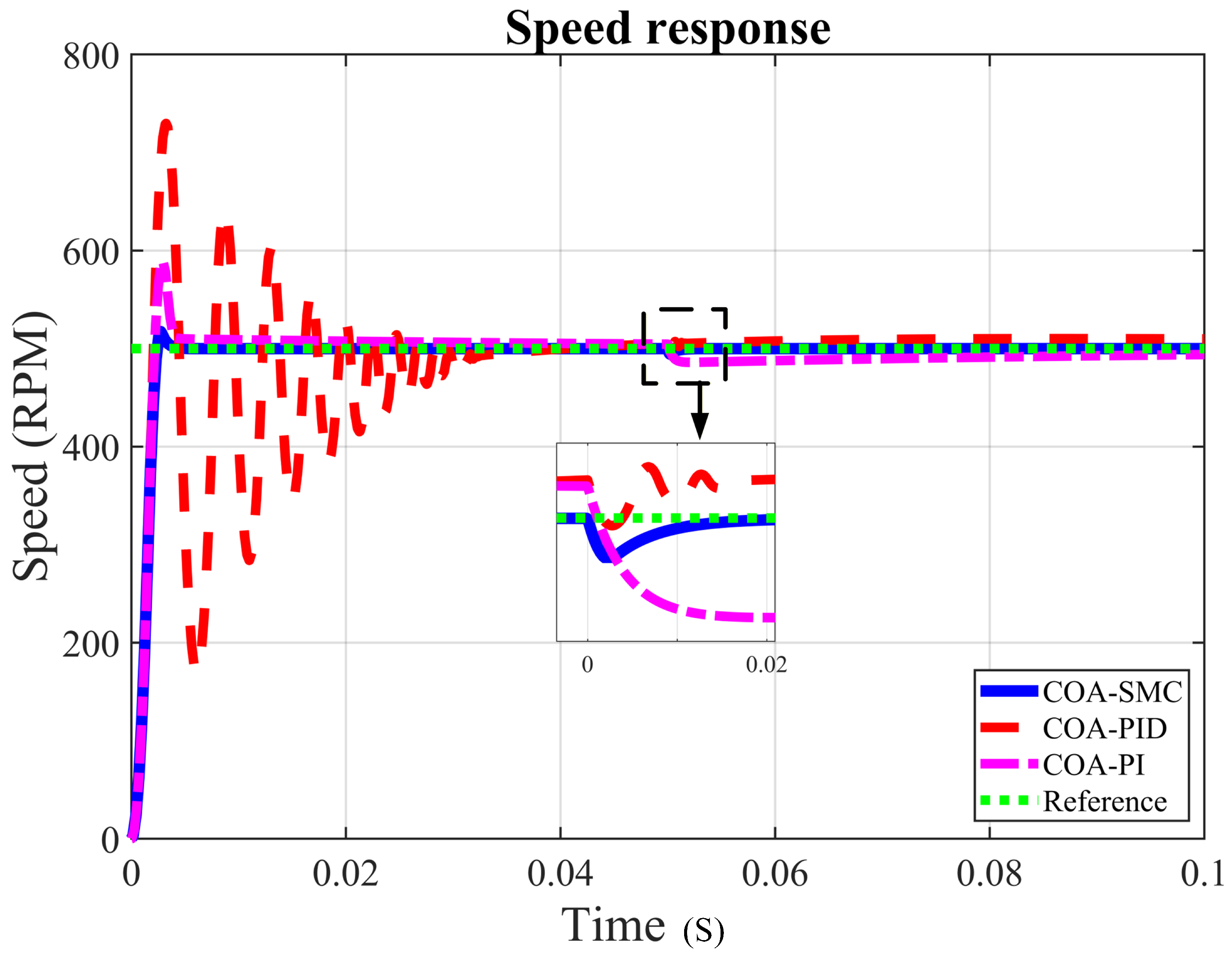
7.3.3. Load Response

Figure 15 shows the transient response upon load application. The sliding mode controller demonstrates the lowest reduction in speed, followed by the PID controller, whilst the PI controller displays the most significant drop in speed under load disturbance.

Table 14. Comparison of MAE and RMSE for different controllers under load conditions.

Controller	MAE	RMSE
SMC	7.0462	51.8287
PID	42.1472	92.1953
PI	14.3450	60.4197

shows that the sliding mode controller achieves the minimal MAE of 7.0462 in performance tracking, signifying that the mean actual speed approximates the reference velocity. It also yields the lowest RMSE of 51.8287, indicating a relatively minor speed deviation. The PI controller provides suboptimal performance, coming in second, with an MAE of 14.3450 and an RMSE of 60.4179, exhibiting moderate divergence from the reference. Conversely, the PID controller exhibits the highest MAE of 42.1472 and RMSE of 92.1953, demonstrating far greater volatility and reduced performance under load circumstances.

7.4. The Comparison of the Different Controllers Using ITSE as Objective Function

7.4.1. Speed Response

To establish a transparent baseline for controller performance comparisons, the classical PI and PID speed controllers were optimized using COA under identical objective criteria. The resulting optimized control loop parameters are listed in

Table 15. PI and PID controllers’ parameter setting using ITAE as objective function.

Controller	Tuned Parameters
	${\mathit{K}}_{\mathit{P}}$	${\mathit{K}}_{\mathit{I}}$	${\mathit{K}}_{\mathit{D}}$
PI	3.8461	66.4894	-
PID	57.6693	508.1322	0.6516

.

Figure 16 shows the transient response, while additional quantitative results are presented in

Table 16. Time-domain response using ITSE as objective function.

Controller	Rise Time (s)	Settling Time (s)	Overshoot (%)	ITSE
SMC	0.001494	0.003068	3.4809	0.1708
PID	0.001333	0.041196	42.8608	4.0212
PI	0.001361	0.004008	17.3791	0.2683

. The sliding mode controller exhibits the best performance with the lowest overshoot at 3.4809%, fastest settling time at 0.003068 s, and lowest ITSE at 0.1708. However, the sliding mode controller has the longest rise time at 0.001494 s. This indicates that the SMC offers superior transient performance and stability.

In contrast, the PID controller demonstrates the fastest rise time at 0.001333 s, but this advantage is accompanied by significantly poorer transient performance; it has the highest settling time, overshoot, and ITSE at 0.041196 s, 42.8608% and 4.0212, respectively, meaning a highly oscillatory and less stable response. Meanwhile, the PI controller has balanced performance with slightly higher overshoot with longer rise time and settling time.

7.4.2. Speed Change Response

Figure 17 shows the transient response when the input speed was changed to 750 rpm at 0.05 s. The PI controller is the fastest to respond to the change of input speed, followed by the PID controller and sliding mode controller. Despite its slightly slower initial response, SMC demonstrates the most stable performance.

Table 17. Comparison of MAE and RMSE for different controllers in speed change response.

Controller	MAE	RMSE
SMC	10.0658	56.8083
PID	48.6196	91.6303
PI	16.5782	57.3911

shows that the sliding mode controller attains the lowest MAE of 10.0658 and the lowest RMSE of 56.8033 regarding tracking accuracy, demonstrating that the actual speed roughly aligns with the reference, exhibiting negligible variation. The PI controller yields a second-lowest MAE of 16.5782 and an RMSE of 57.3911, indicating a marginally greater inaccuracy and moderate divergence. Conversely, the PID controller exhibits the poorest performance., exhibiting the maximum MAE of 48.6196 and RMSE of 91.6303, indicating that its actual speed diverges markedly and erratically from the reference.

7.4.3. Load Response

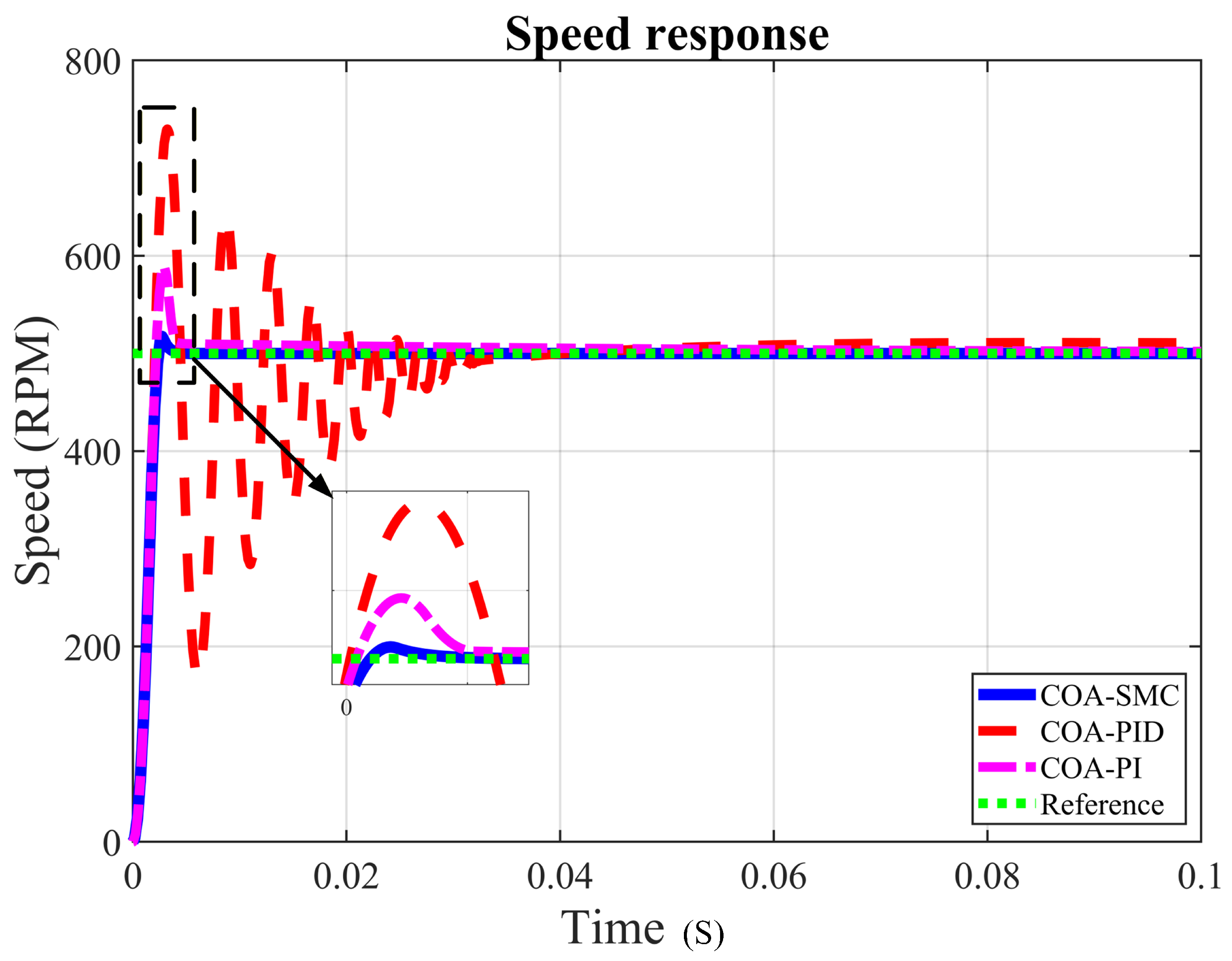
Figure 18 shows the transient response when the load is applied at 0.05 s. The sliding mode controller shows the minimal speed drop, followed by the PID controller, while the PI controller displays the most significant decrease in speed.

Table 18. Comparison of MAE and RMSE for different controllers under load conditions.

Controller	MAE	RMSE
SMC	7.1088	51.7899
PID	36.8773	82.6243
PI	15.7268	52.9923

shows that the sliding mode controller achieves optimal disturbance rejection performance, has the lowest MAE of 7.1088, meaning that the average speed closely approximates the reference, and the lowest RMSE of 51.7899, indicating negligible variance and consistent performance. The PI controller provides second-best performance, with an MAE of 15.7268 and RMSE of 52.9923, indicating considerable variation while preserving satisfactory tracking precision. The PID, on the other hand, demonstrates the least efficacy, with the highest MAE of 36.8773 and RMSE of 82.6243, meaning substantial mistakes and considerable fluctuations during load disturbances.

8. Conclusions

This study evaluated the enhanced speed control of Permanent Magnet Synchronous Motors (PMSMs) using the sliding mode controller, which was optimized by the Chess Optimization Algorithm (COA). The results show that the COA optimizes the sliding mode controller to have better performance in lower overshoot, faster settling time, low speed drop, and has the lowest MAE and RMSE in most scenarios. This means that the COA has optimized the sliding mode controller to be consistently balanced in robustness and error suppression in comparison to HHO and WOA. HHO achieves marginally lower MAE and RMSE than COA, indicating that COA does not outperform the other algorithms uniformly across all test conditions.

For comparison of classical controllers, SMC shows better performance in all conditions, with the lowest overshoot, fast settling time, low MAE and RMSE, and precise tracking in both speed variation and load disturbance scenarios. SMC has disadvantages in rise time. This represents a deliberate trade-off rather than a weakness: the delay is on the order of microseconds, far too small to affect real-world dynamic response in an electric vehicle, whereas the overshoot avoided by SMC corresponds to transient current and torque spikes known to accelerate battery degradation and stress inverter switching devices in conventional controllers. Its stability and robustness make it the most reliable controller overall.

The findings show that COA-optimized SMC achieves an optimal balance of precision, stability, and robustness. Moreover, COA proves to be an effective optimization algorithm, achieving minimal deviation from the reference speed across multiple assessed conditions while offering the most robust and balanced overall multi-objective profile among the three metaheuristics evaluated in this study.

This research was limited to MATLAB/Simulink simulations using an ideal load torque ($T_L$) step input; the results establish a valuable best-case performance baseline. Practical deployment will require an online observer, such as an Extended State Observer, to estimate $T_L$ from measurable signals, which may introduce minor performance degradation relative to simulated bounds. Physically realizing this system demands only standard, highly accessible hardware: a 32-bit industrial digital signal processor (DSP) or microcontroller with a floating-point unit (such as the Texas Instruments C2000 or STM32 series) interfaced with a three-phase voltage source inverter, two current sensors, and a high-resolution encoder for feedback. Future work will leverage these hardware platforms to validate real-time feasibility and traction robustness, focusing on verifying the optimized $ϵ$ and $\delta$ parameters against physical ratings, setting sufficient sampling rates to mitigate discretization chattering, and managing platform switching and thermal constraints.

Note that all optimization results are based on single representative runs of each algorithm. Since COA, HHO, and WOA are stochastic methods, run-to-run variation is present and the presented metrics should be interpreted as representative of the typical behavior of each algorithm rather than as a statistically validated ranking. Multi-seed comparison with statistical significance testing remains a direction for future work.

One of the main directions for future work shall be to scale this optimization framework, having demonstrated the efficiency of the Chess Optimization Algorithm (COA) in tuning and maximizing the baseline performance of a standard boundary-layer SMC. Future work will explore utilizing the unique exploration mechanisms of COA to automatically optimize the advanced control architectures, such as current-constrained continuous nonsingular terminal sliding mode controllers based on control barrier functions (CBFs). Additionally, investigations will be extended to other advanced controllers, including other techniques of sliding mode control, model predictive control (MPC), and hybrid controllers. This is along with next-generation optimization algorithms to further improve dynamic response precision and ensure system robustness in real-world motor applications.

References

- Bashir, M.F.; Pata, U.K.; Shahzad, L. Linking climate change, energy transition and renewable energy investments to combat energy security risks: Evidence from top energy consuming economies. Energy 2025, 314, 134175. [Google Scholar] [CrossRef] [Scilit]
- Nanaki, E.A.; Koroneos, C.J. Climate change mitigation and deployment of electric vehicles in urban areas. Renew. Energy 2016, 99, 1153–1160. [Google Scholar] [CrossRef] [Scilit]
- Chitgreeyan, N.; Pilalum, P.; Marsong, S.; Sonasang, S.; Prabpal, P.; Vo, D.N.; Buayai, K.; Kerdchuen, K.; Kongjeen, Y. Multi-period optimization of energy demand control for electric vehicles in unbalanced electrical power systems considering the center load distance of charging station areas. Eng. Access 2024, 10, 90–102. [Google Scholar] [CrossRef]
- Shriwastava, M.R.; Diagavane, M.; Vaishnav, S. Application Characteristics of Permanent Magnet Synchronous Motors (Case Study). Int. J. Comput. Inf. Sci. 2011, 3, 68–91. [Google Scholar]
- Vlachou, V.I.; Sakkas, G.K.; Xintaropoulos, F.P.; Pechlivanidou, M.S.C.; Kefalas, T.D.; Tsili, M.A.; Kladas, A.G. Overview on permanent magnet motor trends and developments. Energies 2024, 17, 538. [Google Scholar] [CrossRef] [Scilit]
- Wang, Z.; Ching, T.W.; Huang, S.; Wang, H.; Xu, T. Challenges faced by electric vehicle motors and their solutions. IEEE Access 2020, 9, 5228–5249. [Google Scholar] [CrossRef] [Scilit]
- Junejo, A.K.; Xu, W.; Mu, C.; Ismail, M.M.; Liu, Y. Adaptive speed control of PMSM drive system based a new sliding-mode reaching law. IEEE Trans. Power Electron. 2020, 35, 12110–12121. [Google Scholar] [CrossRef] [Scilit]
- Ullah, K.; Guzinski, J.; Mirza, A.F. Critical review on robust speed control techniques for permanent magnet synchronous motor (PMSM) speed regulation. Energies 2022, 15, 1235. [Google Scholar] [CrossRef] [Scilit]
- Choi, A.; Ahn, H.; Chung, Y.; You, K. Sliding Mode Control for Sensorless Speed Tracking of PMSM with Whale Optimization Algorithm and Extended Kalman Filter. Machines 2023, 11, 851. [Google Scholar] [CrossRef] [Scilit]
- Jin, Z.; Sun, X.; Lei, G.; Guo, Y.; Zhu, J. Sliding mode direct torque control of SPMSMs based on a hybrid wolf optimization algorithm. IEEE Trans. Ind. Electron. 2021, 69, 4534–4544. [Google Scholar] [CrossRef] [Scilit]
- Tran, H.N.; Jeon, J.W. Robust speed controller using dual adaptive sliding mode control (DA-SMC) method for PMSM drives. IEEE Access 2023, 11, 63261–63270. [Google Scholar] [CrossRef] [Scilit]
- Suleiman, H.U.; Mu’azu, M.B.; Zarma, T.A.; Salawudeen, A.T.; Thomas, S.; Galadima, A.A. Methods of chattering reduction in sliding mode control: A case study of ball and plate system. In Proceedings of the 2018 IEEE 7th International Conference on Adaptive Science & Technology (ICAST), Accra, Ghana, 22–24 August 2018; pp. 1–8. [Google Scholar] [CrossRef] [Scilit]
- Dai, B.; Xu, F.; Tan, Y.; Sun, J. Enhanced Continuous Terminal Sliding Mode Position Control for PMSM Servo Systems Considering Speed and Current Constraints. IEEE Trans. Energy Convers. 2026; in press. [CrossRef] [Scilit]
- Dai, B.; Wang, Z.; Zhao, J.; Li, S. Critical Current-Constrained Continuous Nonsingular Terminal Sliding Mode Control for PMSM Based on Control Barrier Function. IEEE Trans. Power Electron. 2025, 40, 15093–15103. [Google Scholar] [CrossRef] [Scilit]
- Mishra, S.S.; Jena, C.; Ray, P.K.; Pahadasingh, S. Optimal Frequency Control in Interconnected Power System using Grey Wolf Optimization and Firefly Algorithms. Eng. Access 2024, 10, 143–153. [Google Scholar] [CrossRef]
- Azzawi, H.A.; Ameen, N.M.; Gitaffa, S.A. Comparative performance evaluation of swarm intelligence-based FOPID controllers for PMSM speed control. J. Eur. Des. Syst. Autom. 2023, 56, 475. [Google Scholar] [CrossRef] [Scilit]
- Khanh, P.Q.; Anh, H.P.H.; Thuyen, C.M. Improving PMSM Control Based on Optimizing the Output Membership Function of Fuzzy PI Controller with Weighted Modified Jaya Algorithm. J. Robot. Control 2025, 6, 1938–1948. [Google Scholar] [CrossRef] [Scilit]
- Templos-Santos, J.L.; Aguilar-Mejia, O.; Peralta-Sanchez, E.; Sosa-Cortez, R. Parameter tuning of PI control for speed regulation of a PMSM using bio-inspired algorithms. Algorithms 2019, 12, 54. [Google Scholar] [CrossRef] [Scilit]
- Azeez, M.I.; Abdelhaleem, A.; Elnaggar, S.; Moustafa, K.A.; Atia, K.R. Optimized sliding mode controller for trajectory tracking of flexible joints three-link manipulator with noise in input and output. Sci. Rep. 2023, 13, 12518. [Google Scholar] [CrossRef] [Scilit] [PubMed]
- Nippatla, V.R.; Mandava, S. Performance Analysis of Permanent Magnet Synchronous Motor based on Transfer Function Model using PID Controller Tuned by Ziegler-Nichols Method. Results Eng. 2025, 26, 105460. [Google Scholar] [CrossRef] [Scilit]
- Mohd Zaihidee, F.; Mekhilef, S.; Mubin, M. Robust speed control of PMSM using sliding mode control (SMC)—A review. Energies 2019, 12, 1669. [Google Scholar] [CrossRef] [Scilit]
- Apte, A.; Walambe, R.; Joshi, V.; Rathod, K.; Kolhe, J. Simulation of a permanent magnet synchronous motor using Matlab-Simulink. In Proceedings of the 2014 Annual IEEE India Conference (INDICON), Pune, India, 11–13 December 2014; pp. 1–5. [Google Scholar] [CrossRef] [Scilit]
- Amornwongpeeti, S.; Kiselychnyk, O.; Wang, J.; Shah, N.; Soumelidis, M. Speed control of IPMSM motor drives using Model Reference Adaptive technique. In Proceedings of the 2017 International Conference on Applied System Innovation (ICASI), Sapporo, Japan, 13–17 May 2017; pp. 672–675. [Google Scholar] [CrossRef] [Scilit]
- Wang, H.; Xu, S.; Hu, H. PID controller for PMSM speed control based on improved quantum genetic algorithm optimization. IEEE Access 2023, 11, 61091–61102. [Google Scholar] [CrossRef] [Scilit]
- Sun, Z.; Tian, M.; Li, X. Control Strategy of PMSM for Variable Pitch Based on Improved Whale Optimization Algorithm. Machines 2025, 13, 872. [Google Scholar] [CrossRef] [Scilit]
- Zahraoui, Y.; Zaihidee, F.M.; Kermadi, M.; Mekhilef, S.; Alhamrouni, I.; Seyedmahmoudian, M.; Stojcevski, A. Optimal tuning of fractional order sliding mode controller for PMSM speed using neural network with reinforcement learning. Energies 2023, 16, 4353. [Google Scholar] [CrossRef] [Scilit]
- Zahraoui, Y.; Zaihidee, F.M.; Kermadi, M.; Mekhilef, S.; Mubin, M.; Tang, J.R.; Zaihidee, E.M. Fractional order sliding mode controller based on supervised machine learning techniques for speed control of PMSM. Mathematics 2023, 11, 1457. [Google Scholar] [CrossRef] [Scilit]
- Utkin, V.I. Sliding Modes in Control and Optimization; Springer Science & Business Media: Berlin/Heidelberg, Germany, 2013. [Google Scholar] [CrossRef] [Scilit]
- Alika, R.; Mellouli, E.M.; Tissir, E.H. A modified sliding mode controller based on fuzzy logic to control the longitudinal dynamics of the autonomous vehicle. Results Eng. 2024, 22, 102120. [Google Scholar] [CrossRef] [Scilit]
- Zaihidee, F.M.; Mekhilef, S.; Mubin, M. Application of fractional order sliding mode control for speed control of permanent magnet synchronous motor. IEEE Access 2019, 7, 101765–101774. [Google Scholar] [CrossRef] [Scilit]
- Li, K.; Ding, J.; Sun, X.; Tian, X. Overview of sliding mode control technology for permanent magnet synchronous motor system. IEEE Access 2024, 12, 71685–71704. [Google Scholar] [CrossRef] [Scilit]
- Feng, L.; Deng, M.; Xu, S.; Huang, D. Speed regulation for PMSM drives based on a novel sliding mode controller. IEEE Access 2020, 8, 63577–63584. [Google Scholar] [CrossRef] [Scilit]
- Mathew K., K.; Abraham, D.M.; Harish, A. Speed regulation of PMSM drive in electric vehicle applications with sliding mode controller based on Harris Hawks optimization. e-Prime Electr. Eng. Electron. Energy 2024, 9, 100643. [Google Scholar] [CrossRef] [Scilit]
- Zhang, X.; Sun, L.; Zhao, K.; Sun, L. Nonlinear speed control for PMSM system using sliding-mode control and disturbance compensation techniques. IEEE Trans. Power Electron. 2012, 28, 1358–1365. [Google Scholar] [CrossRef] [Scilit]
- Yu, L.; Huang, J.; Luo, W.; Chang, S.; Sun, H.; Tian, H. Sliding-mode control for PMLSM position control—A review. Actuators 2023, 12, 31. [Google Scholar] [CrossRef] [Scilit]
- Habil, M.; Anayi, F.; Xue, Y.; Shouran, M. Optimisation of sliding mode parameters using different algorithms to control the position of a linear DC motor. AIP Conf. Proc. 2024, 2816, 140004. [Google Scholar] [CrossRef] [Scilit]
- Soon, C.C.; Ghazali, R.; Jaafar, H.I.; Hussien, S.Y.S. Sliding mode controller design with optimized PID sliding surface using particle swarm algorithm. Procedia Comput. Sci. 2017, 105, 235–239. [Google Scholar] [CrossRef] [Scilit]
- Li, B.; Li, L.; Cai, J.; Wu, Y.; Ding, W. Design of PMSM Speed Control System Based on Optimized ITAE Criterion. In Proceedings of the International Conference of Electrical, Electronic and Networked Energy Systems, Xi’an, China, 18–20 October 2024; pp. 434–445. [Google Scholar] [CrossRef] [Scilit]
- Gupta, S.; Biswas, P.K.; Debnath, S.; Ghosh, A.; Babu, T.S.; Zawbaa, H.M.; Kamel, S. Metaheuristic optimization techniques used in controlling of an active magnetic bearing system for high-speed machining application. IEEE Access 2023, 11, 12100–12118. [Google Scholar] [CrossRef] [Scilit]
- Hodson, T.O. Root mean square error (RMSE) or mean absolute error (MAE): When to use them or not. Geosci. Model Dev. Discuss. 2022, 15, 5481–5487. [Google Scholar] [CrossRef] [Scilit]
Figure 1.
Field-oriented control structure of PMSM.
Figure 2.
Diagram illustrating sliding mode controller.
Figure 3.
Flowchart of Chess Optimization Algorithm.
Figure 4.
Convergence curves of algorithms on ITAE as objective function.
Figure 5.
Convergence curves of algorithms on ITSE as objective function.
Figure 6.
Frequency spectrum of : (a) Full range. (b) Zoomed.
Figure 7.
Speed response with SMC-tuned parameters using ITAE.
Figure 8.
Speed response under reference speed change using ITAE.
Figure 9.
Speed response under load disturbance using ITAE.
Figure 10.
Speed response with SMC-tuned parameters using ITSE.
Figure 11.
Speed response under reference speed change using ITSE.
Figure 12.
Speed response under load disturbance using ITSE.
Figure 13.
Speed response with tuned controller parameters using ITAE.
Figure 14.
Figure 15.
Figure 16.
Speed response with tuned controller parameters using ITSE.
Figure 17.
Figure 18.