Article

Effects of Pin Arrangement on Rubber Melt Mixing in a Pin-Barrel Cold-Feed Extruder: Finite Element Analysis and MEA-BP-Based Flow-Field Parameter Prediction


1
Key Laboratory of Advanced Manufacturing and Automation Technology (Guilin University of Technology), Education Department of Guangxi Zhuang Autonomous Region, Guilin 541006, China
2
Guangxi Engineering Research Center of Intelligent Rubber Equipment, Guilin University of Technology, Guilin 541006, China
*
Author to whom correspondence should be addressed.
Appl. Sci. 2026, 16(14), 6880; https://doi.org/10.3390/app16146880
Submission received: 9 June 2026 / Revised: 2 July 2026 / Accepted: 7 July 2026 / Published: 9 July 2026
(This article belongs to the Section Mechanical Engineering)

Abstract

Pin arrangement significantly affects rubber-melt mixing and extrusion in pin-barrel cold-feed extruders. However, internal flow details are difficult to observe experimentally, and efficient prediction of flow-field parameters remains unavailable. This study used a finite-element model preliminarily validated against measured temperatures, together with particle tracing, to compare configurations with 0, 2, 4, and 6 pins per group. A dataset of 140 pin arrangements was generated by Latin hypercube sampling and numerical simulation. A mind evolutionary algorithm-optimized back-propagation neural network (MEA-BP) was then developed to predict melt volume-averaged temperature and average shear rate. Pins increased melt velocity and shear heating and improved cross-sectional temperature uniformity. Among the four uniform configurations, the 4-pin-per-group configuration showed the fastest reduction in segregation scale with a moderate residence time, achieving a favorable balance between mixing adequacy and processing efficiency. Particle tracing indicated repeated fluid splitting and recombination, whereas further increases in the number of pins yielded limited benefits. Under identical data partitions, network settings, and evaluation conditions, MEA-BP achieved R2 values of 0.957 and 0.872 for temperature and shear-rate prediction, respectively, outperforming GA-BP, PSO-BP, and conventional BP.

1. Introduction

Extrusion technology is a fundamental process in polymer processing and is crucial for producing high-performance materials, with the extruder as the core equipment used to implement it. Owing to their excellent properties, rubber products prepared by extrusion are widely used in numerous fields, including national defense, transportation, industry, agriculture, and medicine [1]. However, due to the inherent limitations of their shear mechanism, conventional single-screw extruders exhibit limited dispersive mixing capability and can no longer meet the growing demands for compound uniformity and overall performance in rubber product manufacturing. Bigio et al. [2] experimentally investigated the mixing performance of a fully flighted single-screw extruder and found that laminar flow predominated in the mixing section, resulting in limited mixing capability. To overcome this limitation, researchers developed single-screw extruders equipped with pins mounted on the screw, which enhance mixing by altering the melt flow path. Rawendaal et al. [3] reported dead zones behind the pins; Yao et al. [4] subsequently designed perforated pins to eliminate these dead zones and improve mixing efficiency, thereby demonstrating the potential of pin structures for enhancing mixing.
Extensive experimental and simulation studies have been conducted on the mixing behavior of pin-type cold-feed extruders. Yabushita et al. [5] and Shin et al. [6] used two-color rubber compounds as tracer materials to compare the mixing performance of pin-type single-screw extruders with that of conventional single-screw extruders, confirming that pins can significantly improve mixing performance. Numerical simulations by Brzoskowski et al. [7] based on a Newtonian fluid model showed that rubber reorientation and stretching induced by pin motion are key factors in improving mixing performance. Schöppner et al. [8] optimized distributive and dispersive mixing by varying the geometry and arrangement of pins, finding that pin geometry had no significant effect on dispersive mixing, while similar enhancement effects were observed for distributive mixing. Wang et al. [9] combined mathematical modeling with finite element simulation to analyze the extensional deformation generated as the fluid flowed around the pins, providing a new approach for estimating extensional rheology and explaining the mixing mechanism. Based on the kinematic theory of fluid mixing, Yao et al. [10] employed a non-Newtonian, non-isothermal, three-dimensional finite element method to calculate the scale of segregation and residence time distribution in pin mixing sections with different axial clearances, and found that the mixing capability varied nonlinearly with axial clearance. These studies provide a basis for the optimal design of pin sections; however, in practical production, pin arrangement schemes still rely heavily on small-batch experiments, and the lack of rapid and accurate methods for predicting flow-field parameters leads to long process-development cycles and high costs.
Polymer melts are generally non-Newtonian fluids, and their extrusion processes involve the interplay of multiple physical factors; therefore, a theoretical framework capable of fully and accurately describing their flow behavior remains lacking [11]. With the development of artificial intelligence technology, researchers have adopted data-driven methods to construct neural networks for the accurate prediction of target parameters. Lubura et al. [12] developed an artificial neural network based on TensorFlow to predict torque variation during rubber vulcanization, achieving a mean absolute percentage error below 1.99%. Uruk et al. [13] combined artificial neural networks, Gaussian process regression, and support vector regression to rapidly estimate torque and curing time in rubber vulcanization characteristics. Yuan et al. [14] used an artificial neural network optimized by self-adaptive particle swarm optimization to predict the stress–strain relationship of nitrile rubber under different hardnesses and loading rates, achieving higher accuracy than traditional neural network models. Robin et al. [15] used an artificial neural network to predict the fatigue life of carbon black-filled natural rubber under different temperatures and load ratios, significantly reducing the workload of fatigue experiments. Sui et al. [16] applied a BP neural network to predict the strength and crack resistance of rubber concrete, achieving high prediction accuracy. Hou et al. [17] established a quality prediction model for internal-thread cold extrusion using a GA-BP neural network, providing a new method for related process research. The BP-ANN model constructed by Xiang et al. [18] achieved an accuracy of 97.3% in predicting the fatigue life of natural rubber composites.
In addition to conventional GA and PSO, real-coded genetic algorithms (RCGAs) and their related extensions have been developed to alleviate issues such as parameter sensitivity and premature convergence that may arise in continuous-parameter optimization. Beklaryan et al. [19] proposed an RCGA combined with fuzzy control, which improved the optimization process by adaptively adjusting GA-related parameters. Peng et al. [20] applied RCGA to modeling multi-relational fuzzy cognitive maps, demonstrating that real-coded evolutionary methods can be used for parameter identification and the modeling of complex systems. The above studies indicate that data-driven models can accurately predict key physical quantities in polymer processing, providing a new approach for the rapid evaluation of pin arrangements in extruders. However, training such models generally requires a relatively large amount of experimental or numerical simulation data, which is often difficult to obtain in sufficient quantity in practical applications, thereby limiting the broader adoption of this approach.
To address this issue, a finite element simulation model validated through comparison with measured temperatures was combined with particle tracing to numerically investigate the effects of pin arrangement on melt mixing characteristics; furthermore, 140 pin configurations were generated using Latin hypercube sampling, and flow-field data extracted from finite element simulations were used to construct a surrogate-model training dataset, based on which a mind evolutionary algorithm-optimized BP neural network (MEA-BP) was developed to predict the volume-averaged melt temperature and average shear rate. The main contributions of this paper are as follows:
  • A three-dimensional non-isothermal transient finite element method, validated against measured temperatures, was used to compare the flow-field temperature and streamline characteristics of four configurations containing 0, 2, 4, and 6 pins per group; subsequently, the mixing performance of each configuration was systematically analyzed using kinematic indices, including the mixing index and scale of segregation, together with particle tracing.
  • Latin hypercube design was used to generate 140 pin arrangement schemes, and finite element simulations were performed to construct the flow-field dataset. Furthermore, a physical aggregation feature encoding method was proposed to transform discrete arrangement patterns into low-dimensional feature vectors, thereby avoiding artificial ordinal assumptions in categorical encoding.
  • An MEA-BP model was developed for the rapid prediction of volume-averaged melt temperature and average shear rate. Unlike GA-BP, which employs selection, crossover, and mutation, and PSO-BP, which uses velocity–position updates, MEA optimizes the initial weights and biases of the BP network through convergence and alienation operations. The four models were compared under identical data partitioning, network settings, and evaluation protocols to assess the effects of different optimization mechanisms on predictive performance and run-to-run stability.
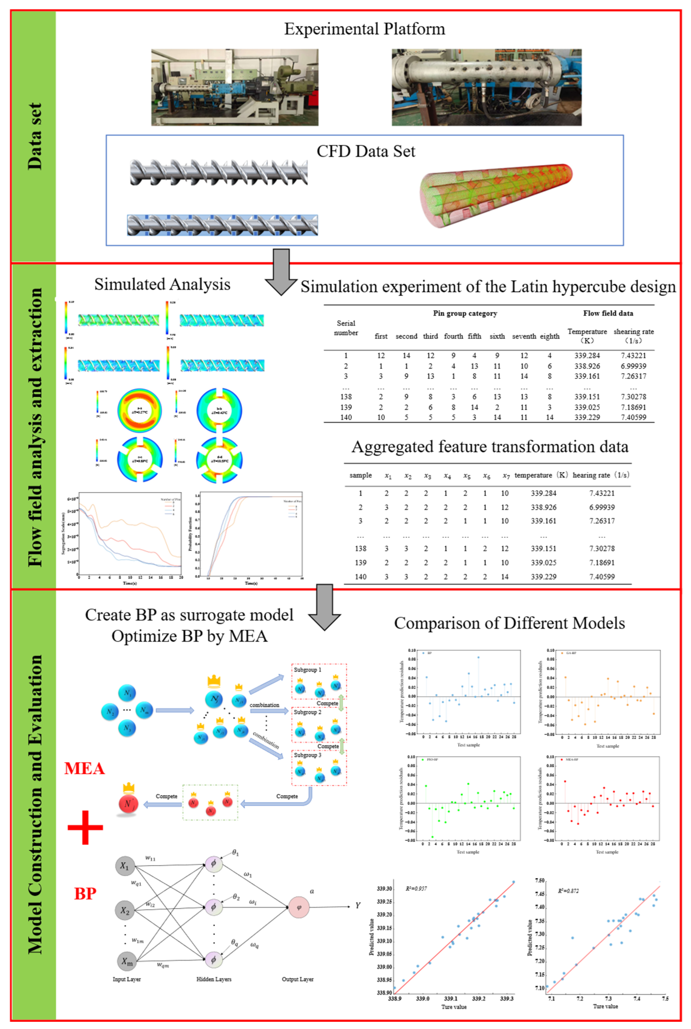
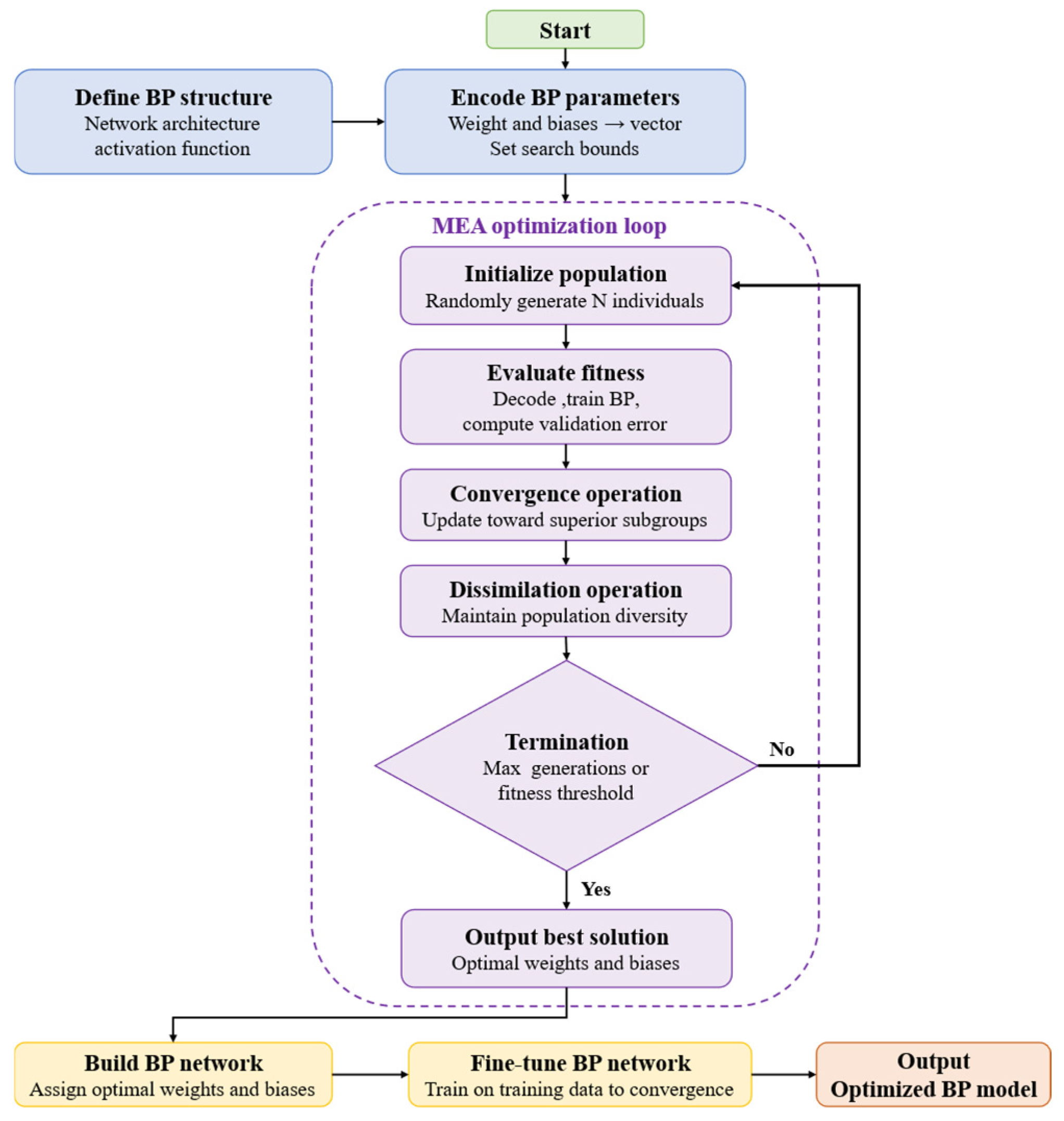
The remainder of this paper is organized as follows: Section 2 describes the parameter settings of the simulation model and analyzes the mixing characteristics of the flow field under different pin arrangements; Section 3 introduces the principles and methodology of the MEA-BP prediction model; Section 4 details the construction process of the MEA-BP model and compares it with GA-BP, PSO-BP, and conventional BP models to evaluate prediction accuracy and stability; and Section 5 summarizes the paper and discusses future research directions. The overall research procedure is shown in Figure 1.

2. Experimental Methods and Analysis of Mixing Characteristics Under Different Pin Arrangements

2.1. Experimental Setup and Fluid-Domain Modeling of the Pin Barrel

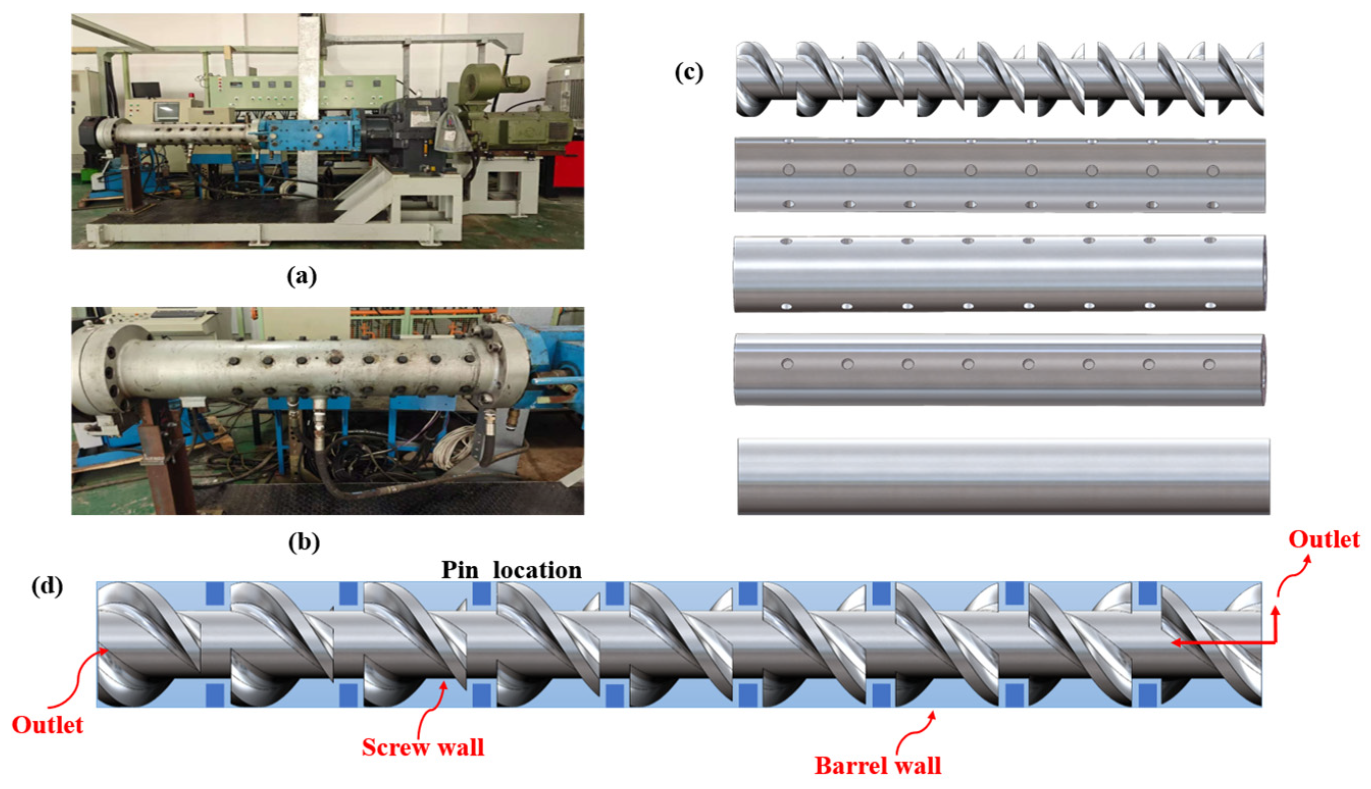
The experimental platform and plasticizing-section model used in this study are shown in Figure 2. Specifically, Figure 2a shows a photograph of the experimental platform; Figure 2b presents the structure of the plasticizing section under the full-pin configuration; Figure 2c shows the fluid-domain models of the screw plasticizing section with four different pin-number configurations, corresponding to 6 (full pins), 4, 2, and 0 pins per group; and Figure 2d shows the flow-field model composed of the pin barrel and screw, with eight groups of pins arranged along the axial direction. Under the full-pin configuration, six pins in each group are uniformly distributed along the circumferential direction, with a pin diameter of 18 mm and a height of 47 mm. In the actual equipment, a gap exists between the pins and the screw surface; to reduce the deviation between simulation and experiment, this gap was set to the measured value of 4.7 mm. Key geometric features, including the outlet, pin location, screw wall, and barrel wall, are also marked in Figure 2d.

2.2. Flow-Field Mathematical Model and Boundary Conditions

Polymer extrusion involves complex interactions among multiple physical mechanisms, such as material deformation, viscous dissipation, and heat conduction [21]. In the present study, ethylene propylene diene monomer rubber (EPDM) was used as the working fluid for the non-isothermal transient flow analysis. The high viscosity of the polymer melt results in a Reynolds number well below unity inside the extruder, indicating that inertial effects are negligible. To simplify the numerical model, the following basic assumptions were made: (1) the melt is an incompressible non-Newtonian fluid; (2) the melt completely fills the entire flow channel; and (3) no slip occurs at the flow-channel walls.
Under the above assumptions, the flow field satisfies the following governing equations of continuum mechanics:
Continuity equation:
u i x i = 0
Momentum equation:
ρ ( u i t + u j u i x i ) + p x i = x i ( η u i x j )
Energy equation:
ρ C p ( T t + u i T x i ) = k 2 T x i 2 + φ
where u i denotes the velocity component in the i-direction; x i denotes the position component in the Cartesian coordinate system; t denotes time; and T denotes temperature.
In this paper, the Bird–Carreau model and an approximate Arrhenius model are adopted to characterize the non-Newtonian rheological behavior of EPDM and its temperature dependence:
η = [ η + ( η 0 η ) ( 1 + λ 2 γ 2 ˙ ) n 1 2 ] e x p [ α ( T T α ) ]
where γ ˙ denotes the shear rate; η 0 denotes the zero-shear viscosity; η denotes the infinite-shear viscosity; λ denotes the relaxation time; n denotes the power-law index; α denotes the temperature sensitivity coefficient; and T α denotes the reference temperature.
However, the present generalized Newtonian model does not explicitly account for viscoelastic effects, pressure-dependent viscosity, wall slip, or rheological variations caused by thermo-mechanical history and changes in rubber formulation. The no-slip boundary condition was adopted as a unified engineering approximation to establish a consistent numerical basis for comparing different pin configurations. Therefore, the present model is intended to evaluate the relative effects of different pin configurations under the investigated operating conditions rather than to provide a universal description of all rubber extrusion processes.
The material property parameters of EPDM are listed in Table 1, and the boundary conditions of the model are given in Table 2.

2.3. Numerical Modeling and Mesh-Independence Validation

To ensure the accuracy and reproducibility of the simulation results, all calculations were performed under the same hardware and software environment. The operating system was 64-bit Windows 10; the CPU was a 12th Gen Intel(R) Core(TM) i5-12600KF operating at 3.70 GHz; the memory was 32 GB; and the graphics card was an NVIDIA GeForce RTX 4060. The numerical solution was carried out using the finite element method (FEM). Flow-field calculations were completed on the ANSYS Polyflow 17.0 platform, and meshing was performed using ANSYS ICEM 17.0.
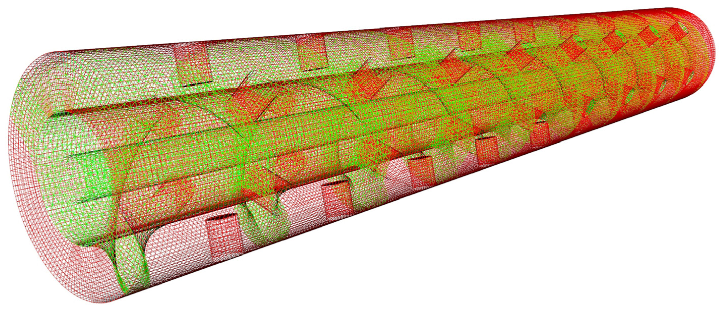
Because the presence of pins makes the flow-channel geometry irregular, the fluid-domain model was meshed using a combination of hexahedral structured grids and tetrahedral unstructured grids. In the region near the pins, tetrahedral unstructured grids were used, and the boundary layer beneath the pins was locally refined to obtain accurate flow-field information in the clearance between the pins and the screw. In addition, because the screw itself has an irregular geometry, its region was independently discretized using tetrahedral grids [22]. To handle the moving boundary caused by screw rotation, the mesh superposition technique (MST) [23] was applied between the fluid domain and the screw, as shown in Figure 3, thereby enabling effective simulation of the dynamic mixing process.
To assess the influence of mesh density on the numerical results and enhance the reliability of the simulations, a mesh-independence study was conducted using coarse, medium, and fine meshes, with shear rate and average temperature selected as evaluation metrics. As shown in Table 3, the relative differences in shear rate and average temperature among the three mesh schemes were below 3%, indicating that these calculated quantities were insensitive to mesh density and met the accuracy requirements for subsequent simulations. On this basis, the simulated temperatures obtained with the medium mesh at different screw rotational speeds were further compared with the measured values. As presented in Table 4, the deviations between the simulated and measured temperatures were below 1.5%, indicating that the model could satisfactorily reproduce the temperature variation in the melt under the investigated conditions. The model was preliminarily validated against temperature data only, whereas its predictions of mixing performance and other extrusion-related indicators have not yet been directly verified experimentally. Considering the results of the mesh-independence analysis and temperature comparison, the medium mesh containing 3.5 × 10⁵ elements was selected as the baseline mesh for subsequent simulations to balance computational efficiency and accuracy.
Numerical simulations were performed using Polyflow 17.0, and its mixing-task module was employed to calculate kinematic parameters, including the mixing index, scale of segregation, and cumulative residence time, for comparing the relative mixing characteristics of different pin configurations under the investigated conditions.
The mixing index is used to characterize the extent of melt breakup during the mixing process and is defined as follows:
M = | D | | D | + | Ω |
where D is the rate-of-deformation tensor; Ω is the vorticity tensor; and the mixing index M reflects the local flow characteristics: when M = 0 , it corresponds to rigid-body flow; when M = 0.5 , it corresponds to shear flow; and when M = 1 , it corresponds to extensional flow.
The scale of segregation is a physical quantity that measures the average size of regions occupied by the same component in a mixture and is used to quantify distributive mixing. It is defined as follows:
S ( t ) = 0 ξ R ( r , t ) d r
where R ( r , t ) is the concentration correlation coefficient between two points separated by a distance r at time t and satisfies R ( 0 , t ) = 1 and R ( ξ , t ) = 0 ; as the mixing effect improves, the scale of segregation S ( t ) decreases accordingly.
The cumulative residence time distribution represents the probability distribution of the time required for the material to be completely extruded under given processing conditions. It is obtained by integrating the residence time density function and is calculated as follows:
G ( t ) = 0 t g ( t ) d t
where g ( t ) denotes the volume fraction of fluid with a residence time within the interval [ t , t + d t ] .

2.4. Melt Mixing Characteristics and Particle-Tracing Analysis Under Different Pin Arrangements

2.4.1. Comparative Analysis of Melt Flow-Field Characteristics

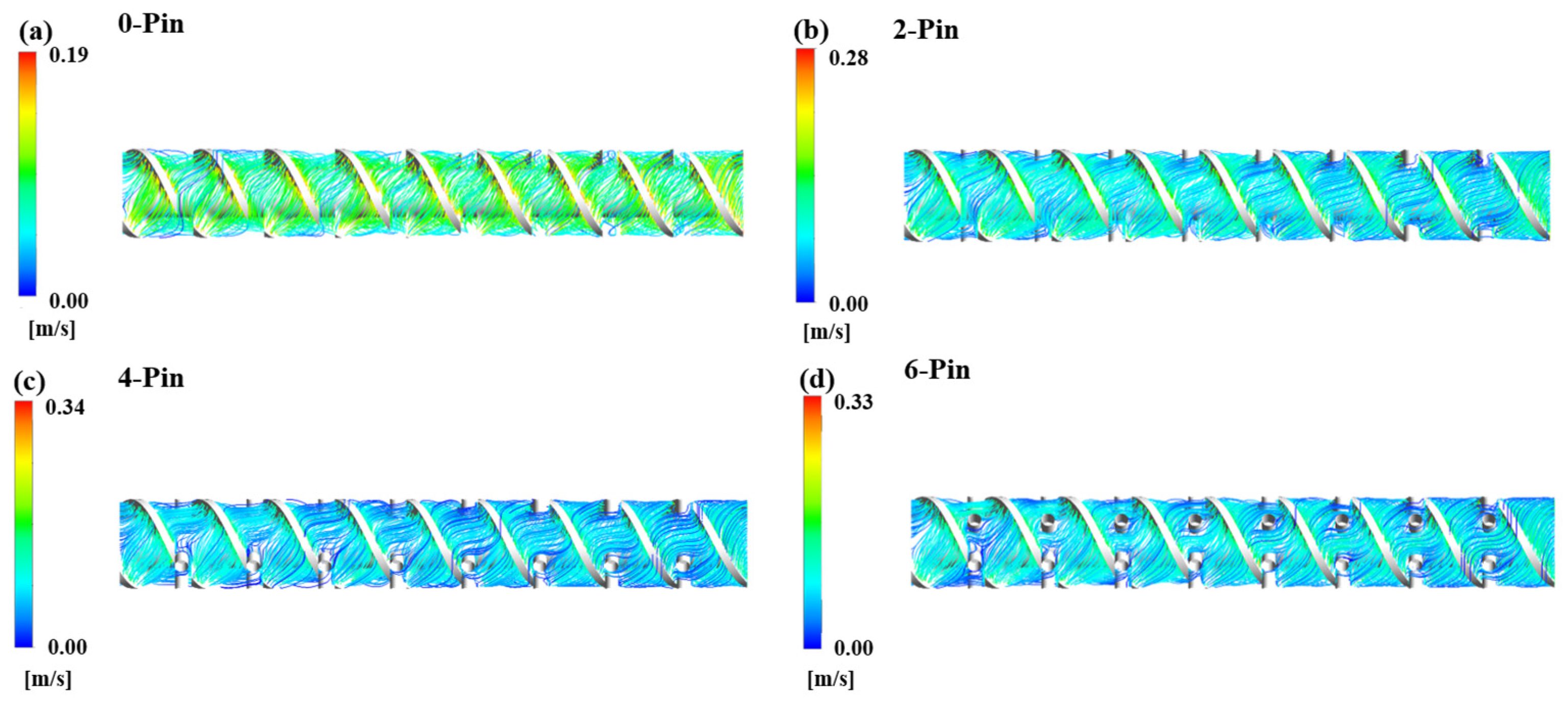
Figure 4 shows the velocity streamlines in the screw channel under different numbers of pins. Without pins, the melt exhibits a stable laminar flow state, with a maximum velocity of 0.19 m/s. After the introduction of pins, obvious flow splitting occurs near the pins, and the melt is forced to change its flow direction under the disturbance of the pin array; the maximum velocities corresponding to 2, 4, and 6 pins per group increase to 0.28, 0.34, and 0.33 m/s, respectively, all higher than that under the no-pin condition. When the number of pins increases to 6 per group, the maximum velocity is slightly lower than that of the 4-pin scheme due to the reduction in the local flow cross-section.
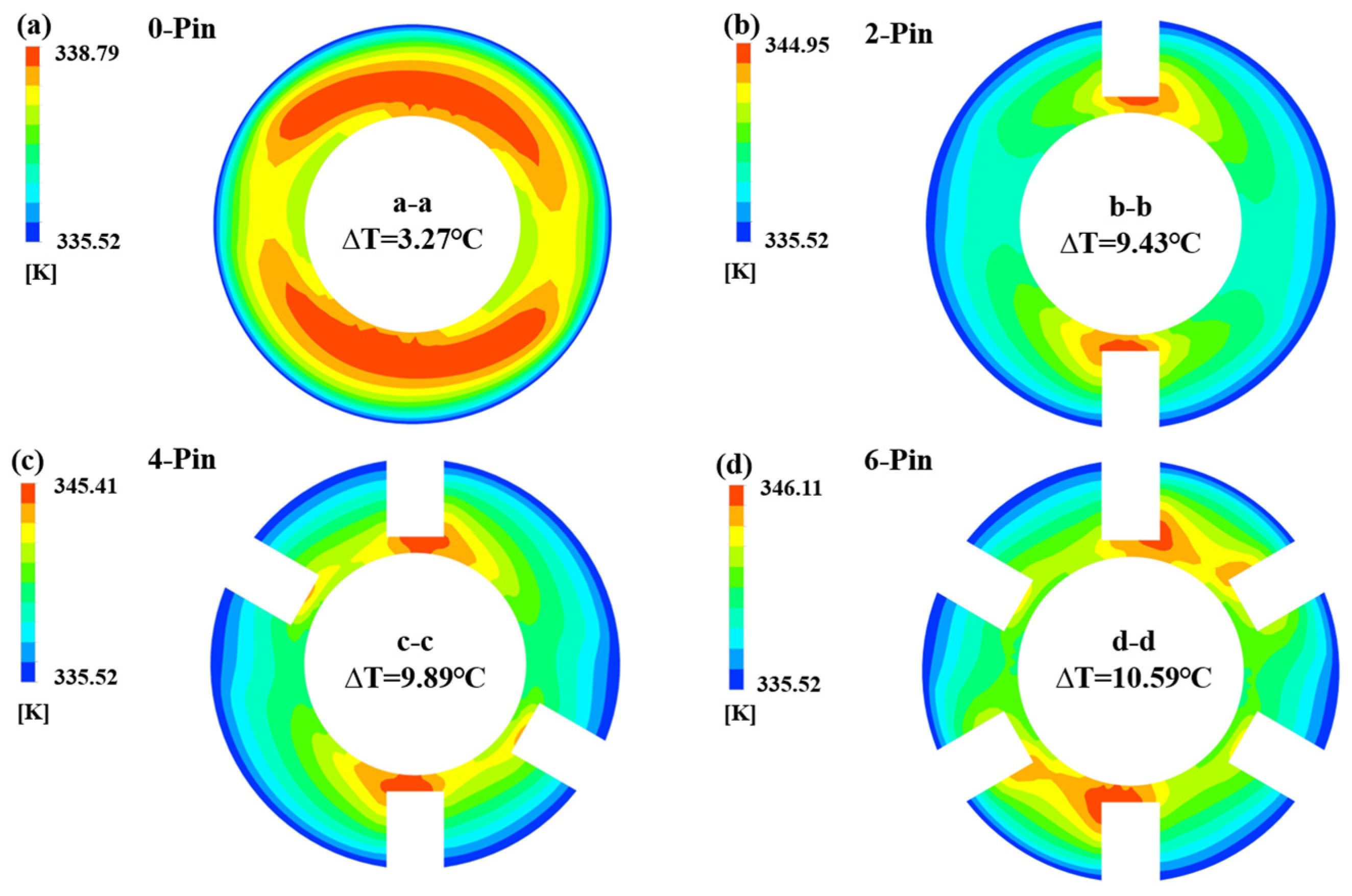
Figure 5 presents the contour maps of the melt cross-sectional temperature distribution under four different pin-number configurations. In the absence of pins, the temperature difference across the section is only 3.27 °C, and the high-temperature region is concentrated in narrow areas on both sides of the screw flight. When the number of pins in each group is 2, the temperature difference increases to 9.43 °C, and the high-temperature region shifts from both sides of the screw flight to the bottom of the pins, with its extent significantly reduced, indicating that the pins effectively enhance local shear heating. When the number of pins increases to 4 and 6, the temperature difference becomes 9.89 °C and 10.59 °C, respectively, and the rate of increase tends to level off. At this stage, although the extreme temperature difference increases slightly, the high-temperature region becomes further concentrated at the bottom of the pins, while the temperature gradient in the remaining cross-sectional regions decreases and the distribution becomes more uniform, which helps suppress local overheating and improve the temperature consistency of the melt. In summary, the introduction of pins enhances the shear-heating effect, causing the high-temperature region to shift from both sides of the screw flight to the bottom of the pins and reducing its affected area, thereby improving the overall temperature uniformity of the flow-channel cross section.
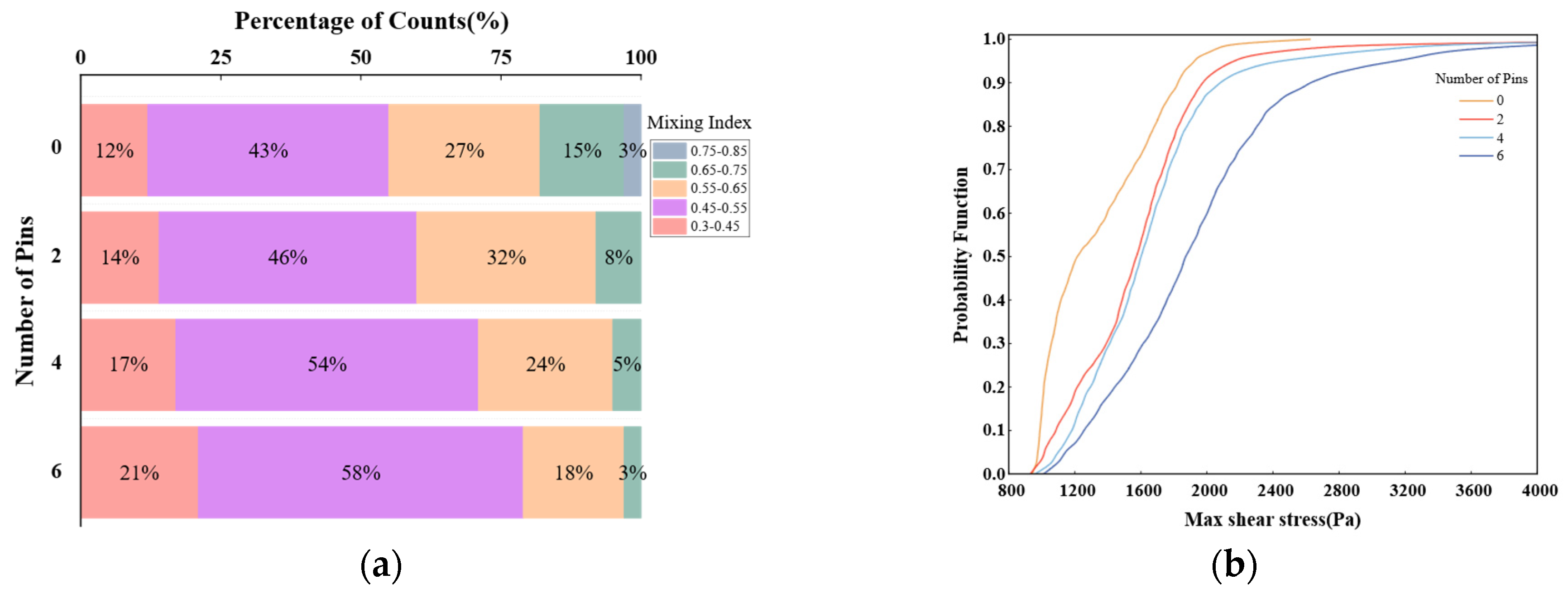
Figure 6a shows the distribution of the mixing index under four operating conditions. Without pins, the mixing index ranges from 0.3 to 0.85; after the introduction of pins, the distribution range narrows to 0.3–0.75, and the proportion within the interval of 0.45–0.55 increases from 43% in the no-pin case to 46% (2 pins), 54% (4 pins), and 58% (6 pins), respectively. To further characterize the intensity of shear flow, Figure 6b presents the maximum shear stress curves for four different pin numbers, where a curve located further to the right indicates a greater shear stress. It can be observed from the figure that the maximum shear stress is the smallest in the absence of pins, increases significantly after pins are introduced, and rises further with increasing pin number.
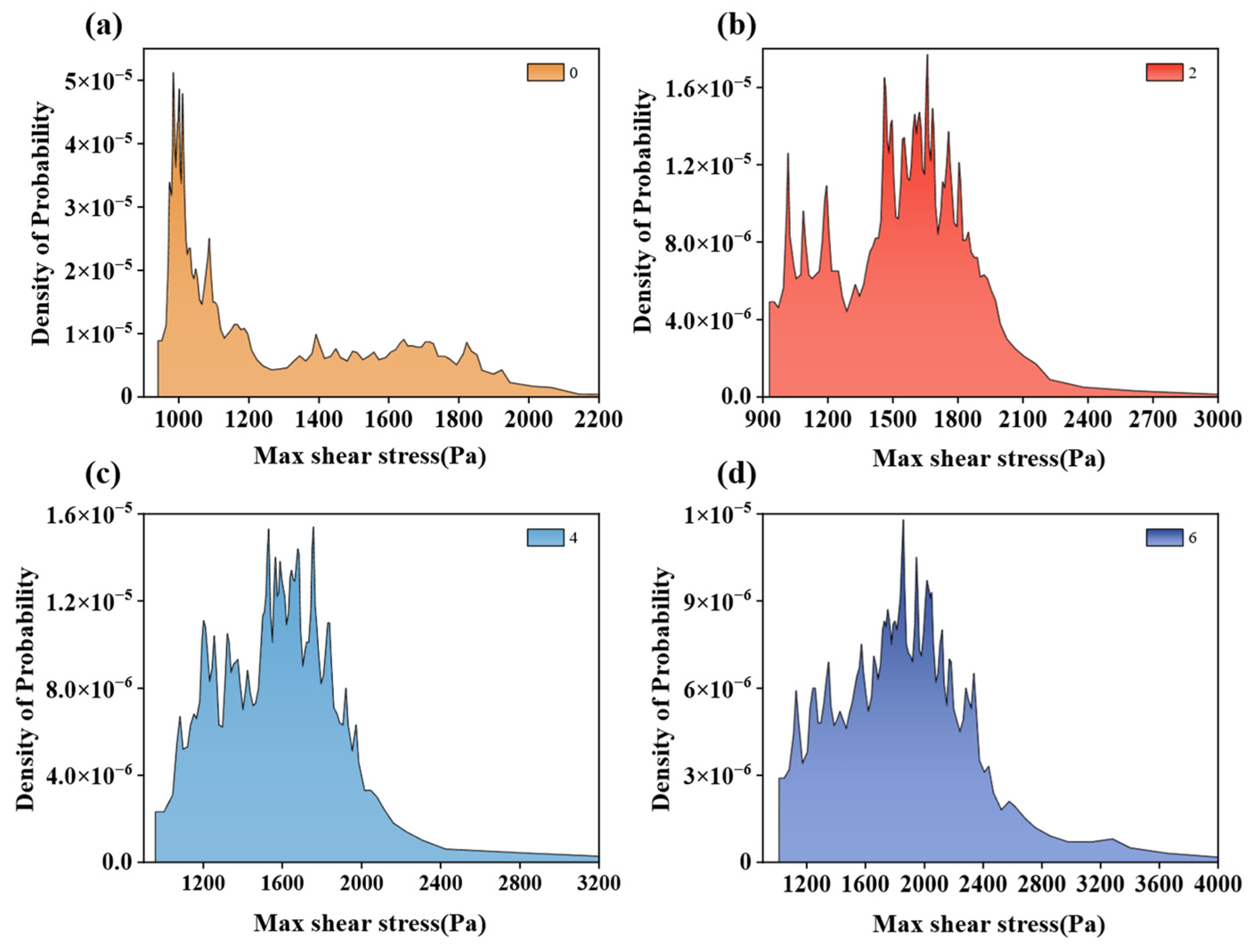
Figure 7 further presents the statistical distribution of the maximum shear stress in the form of a probability density. In the absence of pins, the maximum shear stress is concentrated in the range of 1000–2000 Pa; under the 2-pin, 4-pin, and 6-pin conditions, the main distribution intervals expand to 1200–2100 Pa, 1200–2400 Pa, and 1200–2800 Pa, respectively. These results indicate that the pins effectively increase the overall maximum shear stress in the flow channel, and the magnitude of the increase becomes greater as the number of pins rises. This result is consistent with the trend in Figure 6a, where the mixing index becomes concentrated in the shear-dominated interval, jointly indicating that pins can effectively enhance the shear action within the flow channel.
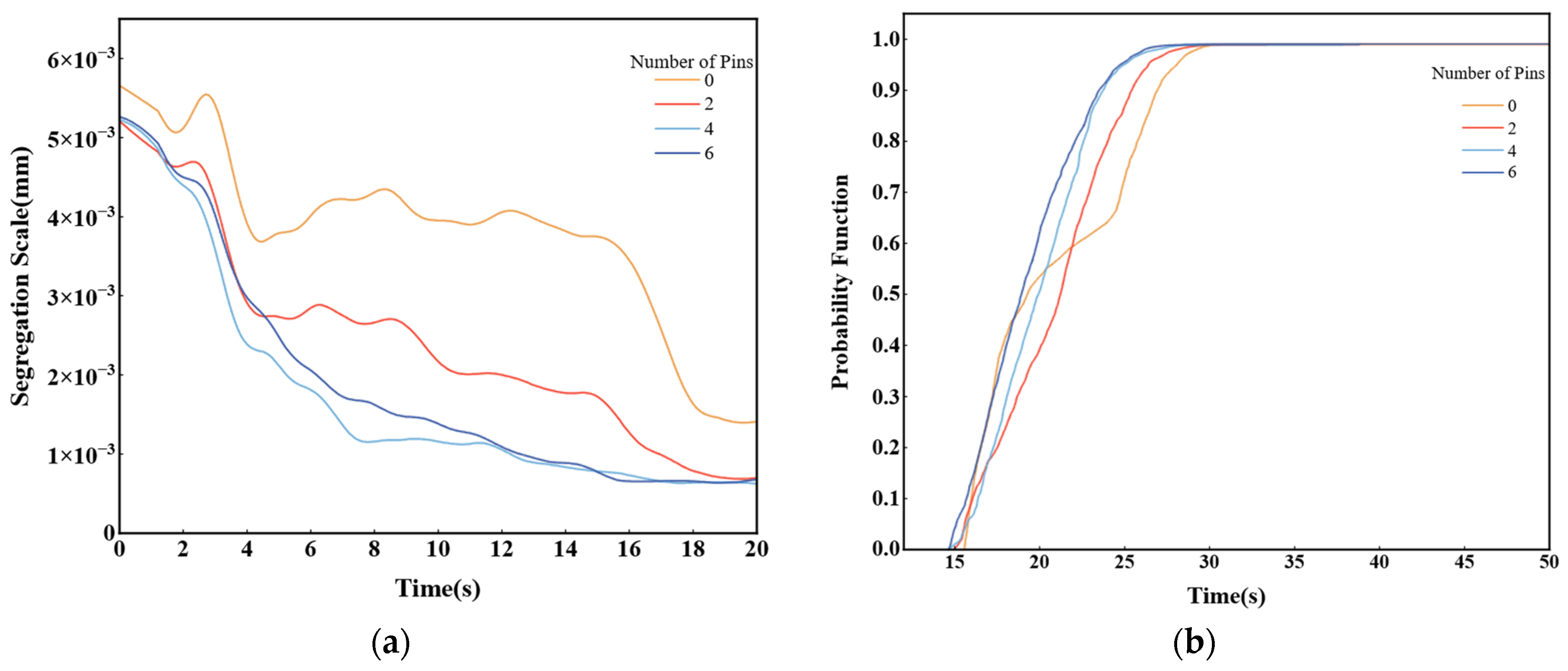
Figure 8 shows the scale of segregation and cumulative residence time curves of the melt under different pin-number configurations. It can be observed from Figure 8a that, without pins, the reserved installation clearances for the pins on the screw cause melt backflow, resulting in an upward trend of the scale of segregation in the middle section, which is detrimental to the improvement of distributive uniformity. When the number of pins in each group increases to 4 and 6, these clearances are occupied by the pins, and the scale of segregation decreases overall, with mixing performance progressively enhanced. The scale of segregation under the no-pin condition is much larger than that under the pin-equipped conditions, further confirming the necessity of introducing pins to improve distributive mixing. Among the three pin-equipped schemes, the configuration with 2 pins per group exhibits the largest scale of segregation; the final scales of segregation for the 4-pin and 6-pin configurations are similar, but the 4-pin scheme shows a significantly faster rate of decline, indicating that it can achieve a comparable level of distributive uniformity in a shorter time.
Figure 8b shows the corresponding cumulative residence time distribution curves, where a curve located further to the right indicates a longer residence time of the material in the flow channel. The cumulative residence time is longest under the no-pin condition because, in the laminar flow state, the melt advances smoothly along the screw axis and lacks transverse disturbance and flow-direction reorientation. After the introduction of pins, the melt undergoes repeated splitting and recombination between the pins, which increases the axial flow velocity and consequently shortens the residence time. Among them, the cumulative residence time curves for the 4-pin and 6-pin conditions show essentially consistent trends.
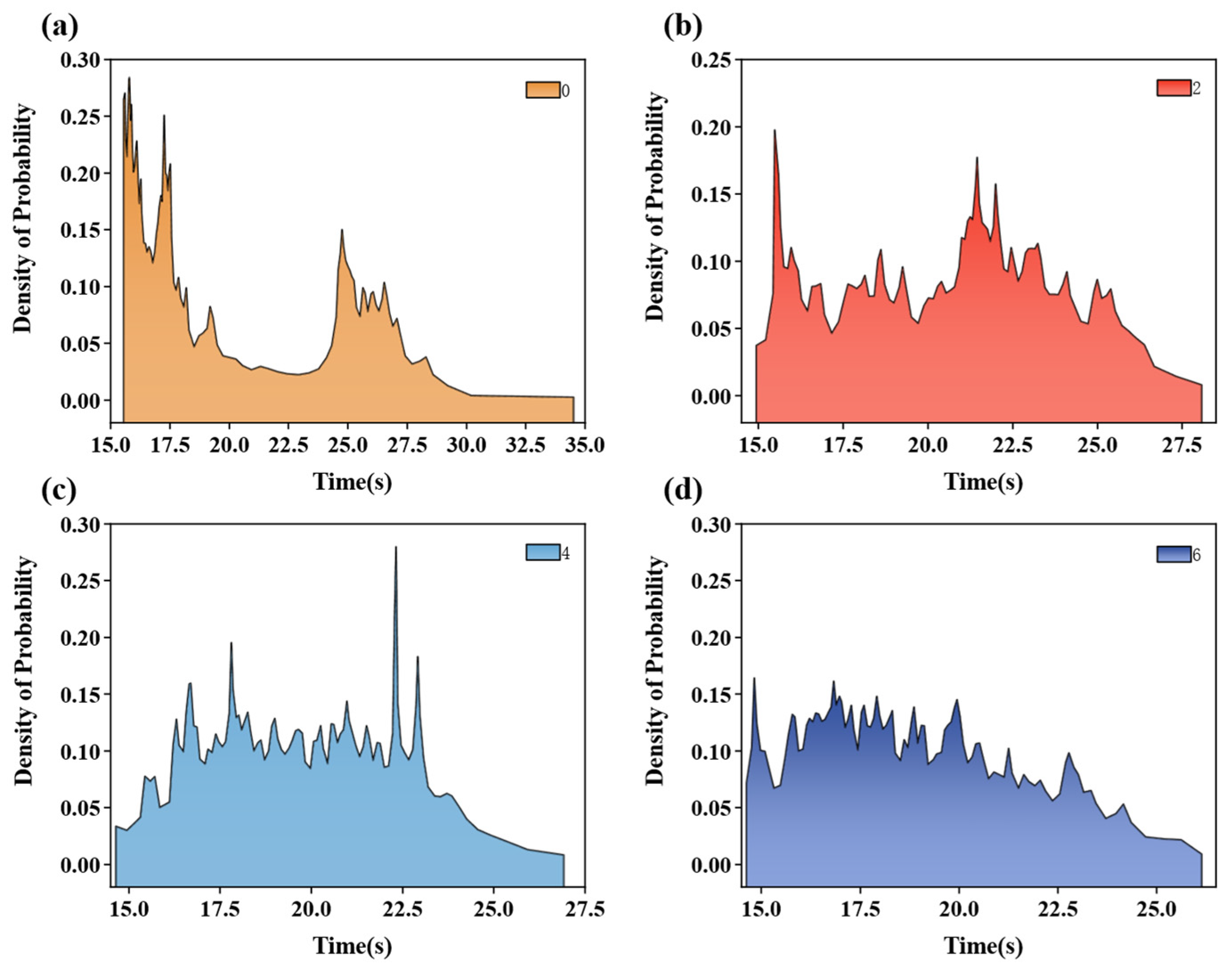
The statistical distribution ranges of residence time under different operating conditions are shown in Figure 9. The range is 15–35 s without pins and decreases to 15–27.5 s, 15–27 s, and 15–26.5 s for configurations with 2, 4, and 6 pins per group, respectively. It can therefore be seen that the residence time shows a slight decreasing trend as the number of pins increases. It should be noted that residence time is not necessarily better when it is either shorter or longer; an excessively short residence time may lead to insufficient mixing, whereas an excessively long residence time may cause material crosslinking and reduce production efficiency. Considering both the scale of segregation and cumulative residence time, the configuration with 4 pins per group achieves the fastest decrease in the scale of segregation while maintaining a moderate cumulative residence time, thereby balancing mixing sufficiency and processing efficiency. Although the configuration with 6 pins per group has a shorter residence time, its decrease rate of the scale of segregation is lower than that of the 4-pin scheme, indicating relatively insufficient mixing efficiency. Therefore, among the four uniform pin configurations investigated in this study, the arrangement with four pins per group exhibited a favorable overall balance between mixing adequacy and processing efficiency.

2.4.2. Tracer-Particle Trajectory Analysis

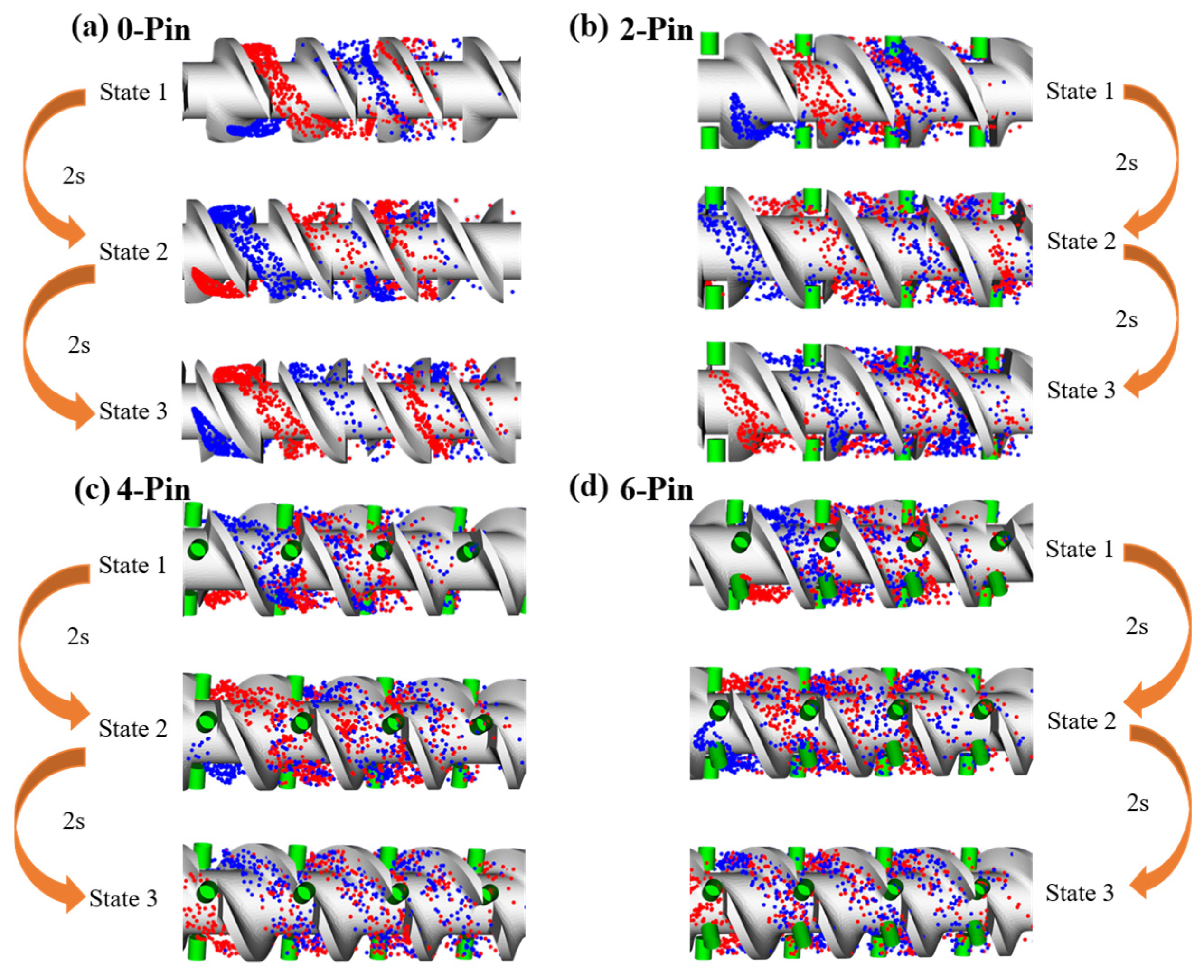
To further investigate the effects of pin arrangement on the melt flow pattern and mixing performance within the screw, particle tracing technology was employed to track and analyze particle motion and the mixing process, as shown in Figure 10. At the initial moment, 2000 tracer particles were released at the inlet of the fluid domain, with the two colors accounting for half each, and their trajectories were subsequently observed during screw rotation. As the flow time progressed, particles of different colors gradually mixed with one another. States 1, 2, and 3 in the figure correspond to the spatial distributions of particles after 8 s, 10 s, and 12 s of screw rotation, respectively.
Figure 10a shows that, in the absence of pins, most particles move along the axial direction, and particle agglomeration remains significant even when the flow time is extended. This indicates that mixing is evidently suppressed under a simple laminar-flow state. After pins are introduced [Figure 10b], the laminar flow is disrupted by disturbances, and particle agglomeration is significantly reduced. Figure 10c further shows that the pins force the melt to undergo repeated splitting and recombination; as the mixing time increases, the splitting effect becomes stronger, thereby enhancing the mixing performance. When the number of pins increases to 6 per group [Figure 10d], the splitting and mixing effects are not significantly enhanced compared with the 4-pin scheme, and the degree of improvement gradually decreases with increasing mixing time. In summary, pins can significantly improve the mixing capability of the screw, but once a certain number is reached, the enhancement effect of adding more pins tends to become limited.
The above analysis shows that pin arrangement has a significant influence on mixing performance, and that clear differences exist among different schemes. However, a single three-dimensional non-isothermal transient simulation is time-consuming, and if all possible arrangement combinations are simulated exhaustively, the computational cost will be prohibitively high. On the other hand, engineering practice places greater emphasis on the rapid evaluation of key flow-field parameters such as temperature and shear rate. Therefore, it is necessary to construct a surrogate model based on finite element simulation data that can efficiently predict flow-field characteristics.

3. Principles and Methodology of the MEA-BP Prediction Model

3.1. Mind Evolutionary Algorithm (MEA)

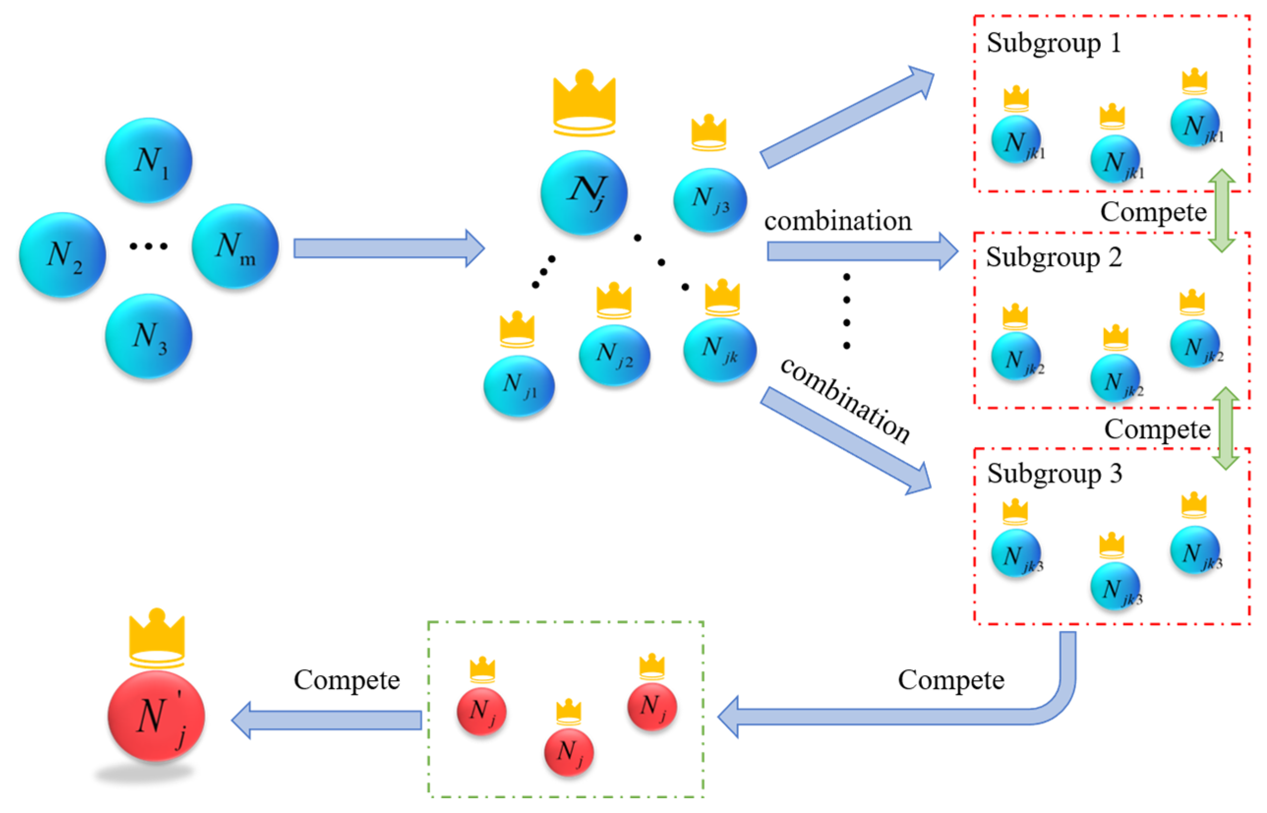
Inspired by the evolutionary process of human thinking, the Mind Evolutionary Algorithm (MEA) is a heuristic optimization approach developed to mitigate premature convergence and enhance the global-search efficiency of conventional genetic algorithms (GAs) [24]. Building on the GA concepts of population, individuals, and environment, this algorithm introduces mechanisms such as subpopulation division, bulletin-board-based information sharing, and convergence and dissimilation operations, thereby enhancing global optimization capability through competition and cooperation among subpopulations. MEA first divides the population into superior subpopulations and temporary subpopulations, then performs convergence operations within subpopulations and dissimilation operations among subpopulations, while using a bulletin board for information exchange, thus rapidly approaching the global optimum. The main steps of the algorithm are as follows:
  • Step 1: A certain number of individuals are randomly generated in the solution space. Their scores are calculated according to the scoring function, superior individuals and temporary individuals with higher scores are selected, and their positions and scores are recorded on the local bulletin board.
  • Step 2: Taking the superior individual N j ( 1 j m ) and the temporary individuals as centers, new individuals N j 1 , N j 2 , , N j k with potential advantages are generated, thereby forming a certain number of superior subpopulations and temporary subpopulations for the subsequent screening stage.
  • Step 3: New winners are generated through competition within each subpopulation, and this process is referred to as convergence. During convergence, the variance of the normal distribution is used as an adaptive adjustment function to search for high-scoring individuals within the subpopulation and assign the corresponding score to the group to which they belong. The variance of the distances among the winning individuals published on the global bulletin board is defined by the following formula:
    δ ( i + 1 ) d = c 1 δ i d + c 2 δ
    where c 1 and c 2 are selectable constants, and δ is the evolutionary distance between the winning individuals of two generations.
  • Step 4: When no new winning individuals are generated in any subpopulation, the scores of all subpopulations are calculated and recorded on the bulletin board. The subpopulations then compete again through operations such as replacing, recombining, or discarding low-scoring subpopulations, and participate once more in global selection until the globally optimal individual A is obtained. The overall evolutionary process of MEA is shown in Figure 11.
To clarify the optimization of BP network parameters by MEA, the connection weights and biases of the BP network were jointly encoded into a decision vector X . Let W 1 and b 1 denote the weights and biases from the input layer to the hidden layer, respectively, and let W 2 and b 2 denote the weights and biases from the hidden layer to the output layer, respectively, then:
X = vec W 1 T , vec W 2 T , b 1 T , b 2 T T
For the i -th sample in the training set, the predicted output of the BP network can be expressed as:
y ^ i = W 2 f W 1 x i + b 1 + b 2
Here, x i and y ^ i denote the input and predicted output of the i -th sample, respectively, and f ( ) represents the transfer function of the hidden layer. MEA takes the mean squared error between the predicted and target outputs of the training set as the optimization objective:
min X F ( X ) = 1 N i = 1 N y ^ i y i 2 2
Here, N denotes the number of training samples, and y i represents the target output of the i -th sample.
To accommodate the maximization search process of MEA, the objective function was transformed into a fitness function:
Fit ( X ) = 1 1 + F ( X )
Therefore, maximizing the fitness function is equivalent to minimizing the prediction error of the BP network on the training set. The optimal individual obtained by MEA is decoded into the initial weights and biases of the BP network and is then used for subsequent training.

3.2. BP Neural Network

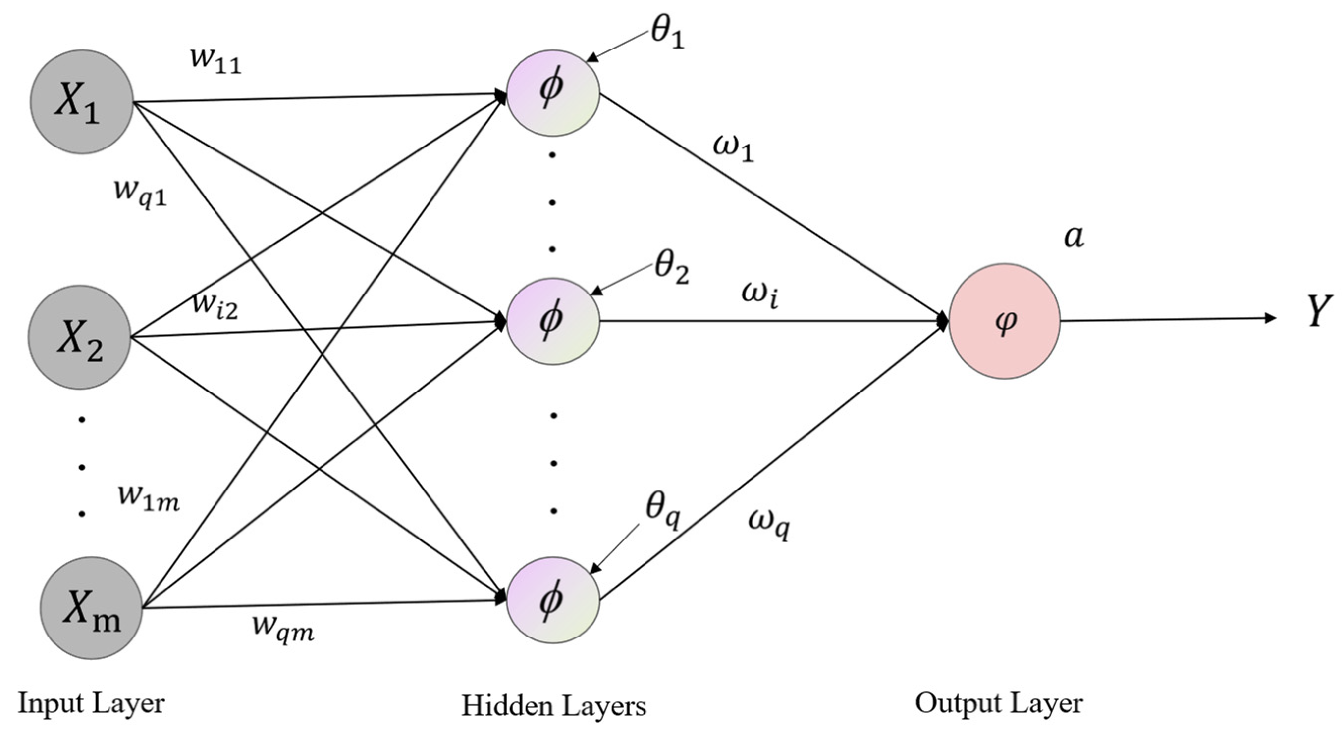
The BP neural network is a supervised learning model based on error backpropagation and has been widely applied in engineering fields owing to its mature theoretical foundation, clear computational procedure, and excellent nonlinear mapping and learning capabilities [25,26,27,28]. The network is composed of input, hidden, and output layers, with a fully connected architecture across layers and no lateral connections among neurons within an individual layer [29]. During training, the weights and thresholds are first initialized; the input samples are then transmitted layer by layer through forward propagation and reach the output layer after calculation by the activation function; if the output error exceeds the preset accuracy, the network enters the backpropagation stage, in which the error signal is propagated backward through the network, the gradients of the error with respect to the weights and thresholds are calculated layer by layer, and the parameters are updated along the gradient descent direction before forward propagation is performed again. This iterative process is repeated until the error converges within the allowable range, and an output satisfying the accuracy requirement is finally obtained. The topology of this network is shown in Figure 12.
The input of the hidden layer can be written as follows:
u i = i = 1 M ( w i j x j ) + θ i
where u i denotes the input to the hidden layer and w i j and C represent the connection weights and thresholds between the input layer and the hidden layer, respectively, where i = 1 , 2 , , q , j = 1 , 2 , , m .
The output of the hidden layer can be written as follows:
y i = Φ ( u i )
where y i denotes the output of the hidden layer, and Φ denotes the transfer function of the hidden layer.
The input of the output layer can be written as follows:
v = i = 1 a ( w i y i ) + a
where v denotes the input to the output layer, w i represents the weights between the output layer and the corresponding hidden layer, and a denotes the threshold of the output layer.
Accordingly, the output of the output layer can be determined as follows:
o = φ ( v ) = φ { i = 1 q w i Φ [ i = 1 M ( w i j x j ) + θ i ] + a }
where o denotes the output of the output layer, and φ denotes the transfer function of the output layer.
Although BP neural networks possess excellent nonlinear mapping capability, good fault tolerance, and adaptability, their gradient-descent-based training mechanism often leads to problems such as slow convergence and susceptibility to local minima, while the network also faces potential risks of overfitting and underfitting [30]. In addition, the network is highly sensitive to the selection of initial weights and thresholds, and improper random initialization may lead to unstable solution quality, thereby reducing the generalization performance and training efficiency of the model [31]. Therefore, obtaining an appropriate set of initial weights and thresholds before training a BP neural network is crucial.

3.3. MEA-Optimized BP Neural Network

The MEA-BP model integrates the global optimization capability of MEA with the nonlinear mapping ability of the BP neural network, leading to improvements in both training efficiency and prediction accuracy [32]. The MEA-BP algorithm selects the optimal individual on the bulletin board through continuous convergence and dissimilation operations of subpopulations, and decodes it into the initial weights and thresholds of the BP network according to the encoding rules, thereby improving the network’s convergence speed and global optimization capability. The algorithmic procedure of MEA-BP is shown in Figure 13, and its main steps are as follows:
  • Data preparation and network configuration: Construct the training and test datasets, and specify the topological structure of the BP neural network.
  • MEA parameter initialization: Set the principal control parameters of the algorithm, including the iteration limit, total population size, and the number of individuals assigned to the superior and temporary subpopulations.
  • Population initialization and candidate evaluation: Construct the initial population using random sampling, assess the fitness of all individuals, and assign the best-performing candidates to the superior and temporary groups.
  • Formation of subpopulations: Construct two categories of subpopulations around the selected candidates, with the superior and temporary individuals serving as the centers of the corresponding groups.
  • Convergence and alienation operations: Search for local optima through internal evolution within each subpopulation, and then promote competition among subpopulations so that well-performing groups are retained while inferior groups are removed.
  • Iterative search for the optimal solution: Continue the convergence and alienation processes until the maximum number of iterations is attained or the fitness value of the best candidate stabilizes.
  • Initialization of network parameters: Decode the best candidate retained on the bulletin board to determine the initial weights and thresholds of the BP neural network.
  • BP neural network training: the BP network is trained using the optimal initial parameters until the stopping criterion is satisfied, and the final prediction results are then output.

4. Development and Performance Evaluation of the MEA-BP-Based Flow-Field Parameter Prediction Model

4.1. Design of Pin-Arrangement Schemes and Dataset Construction

During rubber extrusion processing, the viscoelasticity of the rubber compound directly determines its flowability, which is closely related to temperature and shear rate [33]. Therefore, to investigate the relationship between pin arrangement and extrusion performance, this study constructs a neural network prediction model using the arrangement of pins in each group as the input and the volume-averaged temperature and shear rate of the fluid domain as the outputs.
In the actual extruder barrel, each pin-group cross section is preset with six equally spaced angular holes, with circumferential angles of 0°, 60°, 120°, 180°, 240°, and 300°. Under this geometric constraint, this study summarizes 14 typical pin installation patterns, covering various numbers and angular distributions from no pins to full pins, as shown in Table 5.
To achieve as uniform a sampling as possible within the design space formed by combinations of discrete patterns across eight axial pin groups under a limited number of simulations, a discrete sampling method based on Latin hypercube sampling (LHS) was employed to generate 140 pin configurations [34]. Specifically, 140 continuous sample points were first generated in the eight-dimensional unit hypercube [0, 1]8, with each dimension corresponding to one axial pin group. The coordinate in each dimension was then mapped to the local pattern index of the corresponding pin group according to 14 equally spaced intervals. When duplicate combinations of the eight group patterns occurred after discrete mapping, new candidate samples were generated and remapped until 140 unique pin configurations were obtained.
To examine the distribution of the discrete samples across the axial pin groups, the occurrence frequencies of the 14 local patterns were counted among the 140 samples for each pin group. The results showed that each of the 14 local patterns occurred 10 times among the 140 samples of every axial pin group, indicating balanced marginal occurrence frequencies at the individual pin-group level after discrete mapping. After sample generation, finite element simulations were performed for each pin configuration while keeping the remaining material parameters, geometry, operating conditions, and thermal boundary conditions unchanged, and the volume-averaged melt temperature and average shear rate were extracted as surrogate-model outputs. The set of 140 samples represents a compromise between finite element computational cost and the sampling requirements of the investigated pin-arrangement space, and the resulting model is mainly applicable to the pin-configuration range and operating conditions considered in this study. The specific composition is shown in Table 6.

4.2. Feature Encoding and Data Normalization

If the index of each group (1–14) is directly used as the input to the neural network, an implicit ordinal assumption is introduced, causing the network to incorrectly infer that “the difference between Mode 2 and Mode 3 is smaller than that between Mode 2 and Mode 14,” although such numerical distances have no corresponding physical meaning. In addition, one-hot encoding would generate a 112-dimensional input vector, which is highly prone to overfitting under small-sample conditions [35]. To address this issue, this paper proposes a feature encoding method based on physical-meaning aggregation, which maps the overall configuration of the eight pin groups into a seven-dimensional vector, constructed as follows:
x j = i = 1 8 δ j Θ ( p i ) , j = 1 , , 6
x 7 = i = 1 8 | Θ ( p i ) |
where p i { 1 , 2 , , 14 } denotes the pattern number of the i t h pin group; Θ ( p i ) denotes the set of angular positions corresponding to pattern p i , where i = 1, 2, 3, 4, 5, and 6 correspond to 0°, 60°, 120°, 180°, 240°, and 300°, respectively; | Θ ( p i ) | denotes the number of elements in this set; and δ is an indicator function, which equals 1 when the condition is satisfied and 0 otherwise.
These features are determined entirely by the actual physical arrangement of the pins, avoiding the introduction of artificial sequential relationships unrelated to the physical layout, while reducing the 112-dimensional one-hot-encoded input to seven physically meaningful variables. Table 7 presents examples of aggregated features for selected samples.
To examine whether the aggregated feature representation loses predictive information associated with the axial order of pin groups, an order-preserving binary encoding was further developed as a comparison. Under this representation, each of the eight axial pin groups was described by six binary occupancy variables corresponding to the circumferential positions at 0°, 60°, 120°, 180°, 240°, and 300°. A value of 1 indicates that a pin is installed at the corresponding circumferential position, whereas a value of 0 indicates the absence of a pin. The binary feature vectors of the eight pin groups were then concatenated sequentially according to their actual physical order from the inlet side to the outlet side. Consequently, the resulting feature vector contains 48 variables, explicitly preserving both the circumferential pin distribution within each group and the complete axial arrangement of all groups, and was used as the order-preserving encoding in the subsequent feature-encoding comparison.
Neural networks are highly sensitive to the scale of input features. If the dimensions or numerical ranges of different features vary greatly, imbalanced gradient updates may occur, leading to slow training convergence or even trapping in local optima. To eliminate these effects, min–max normalization was applied to the input data in this study [36], linearly mapping all features to the interval [0, 1], with the normalization formula shown in Equation (15). After model training is completed, the normalized outputs must be restored to their original physical scales; this process is referred to as inverse normalization, as shown in Equation (16):
x n o r m = x x m i n x m a x x m i n
x = x n o r m · ( x m a x x m i n ) + x m i n
where x is the original feature value of the i t h sample; x n o r m is the normalized value ( [ 0 ,   1 ] ); and x m a x and x m i n are the maximum and minimum values of the original data in the training set, respectively.

4.3. Evaluation Metrics and Hyperparameter Optimization for the MEA-BP Model

In this study, model performance was comprehensively evaluated using three metrics: mean absolute error (MAE), root mean square error (RMSE), and the coefficient of determination (R2). MAE represents the mean absolute magnitude of the prediction errors and directly reflects the overall level of prediction deviation. RMSE measures the overall discrepancy between predicted and actual values and is more sensitive to larger prediction errors. Smaller MAE and RMSE values indicate closer agreement between the model predictions and the true values. R2 measures the ability of the model to explain the variation in the target variable, with a value closer to 1 indicating better model fitting performance. The calculation formulas for these metrics are given as follows:
MAE = 1 n i = 1 n | y i y ^ i |
RMSE = 1 n i = 1 n y i y ^ i 2
R 2 = 1 i = 1 n ( y i y ^ i ) 2 i = 1 n ( y i y ¯ ) 2
where y i is the true value of the i t h sample, y ^ i is the corresponding model-predicted value, n is the total number of samples, and y ¯ is the arithmetic mean of all true values.
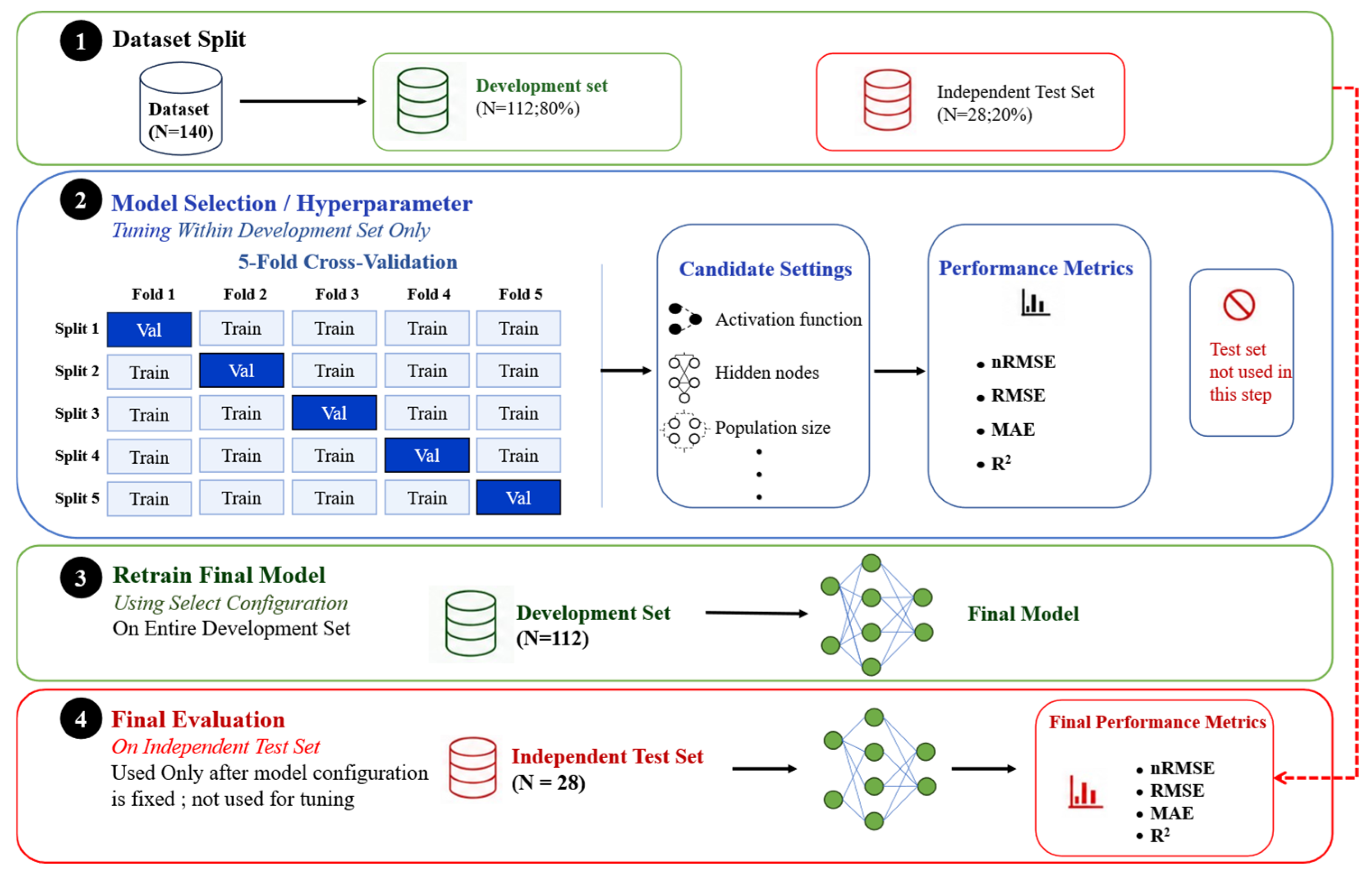
To prevent information leakage between hyperparameter selection and final performance evaluation, the 140 samples were randomly divided into a development set of 112 samples and an independent hold-out test set of 28 samples. The development set was used exclusively for model training and hyperparameter selection; before the model configuration was finalized, the independent hold-out test set was not involved in tuning the network architecture, optimization-algorithm parameters, or random initialization settings. Within the development set, five-fold cross-validation was used to compare candidate activation functions, numbers of hidden-layer neurons, and population sizes for optimization algorithms, including GA, PSO, and MEA. For each cross-validation fold, normalization parameters were fitted only using the corresponding training subset and then applied to its validation subset. The optimal model configuration was then determined according to the average performance across the five folds, and the final model was retrained using all development-set samples. Finally, the trained model was applied to the independent hold-out test set, and its generalization performance was evaluated using the coefficient of determination, root mean square error, mean absolute error, and mean absolute percentage error. The detailed procedure is illustrated in Figure 14.
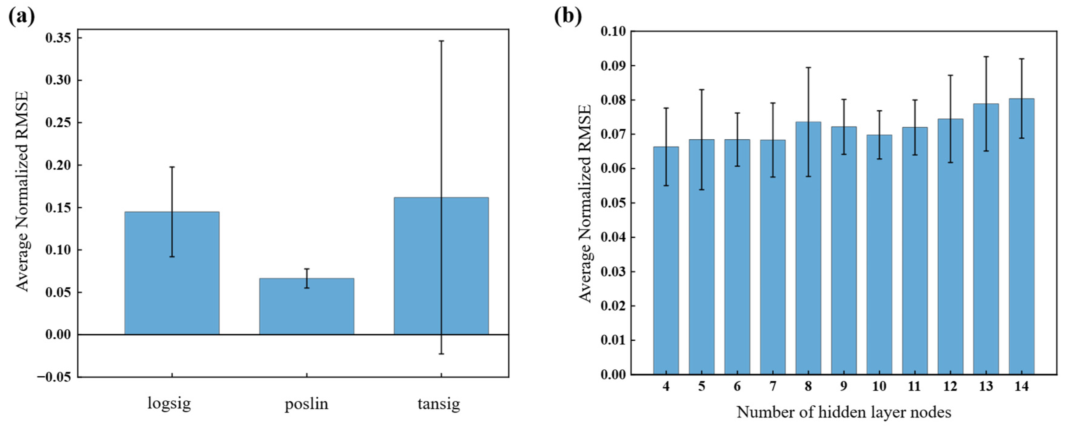
Based on the above evaluation metrics, the key hyperparameters of the BP neural network were further optimized in this study. The hidden-layer activation function is an important factor affecting model performance, and commonly used functions include tansig, poslin, and logsig [37]. As shown in Figure 15a, under the same development-set split, training settings, and candidate range of hidden-layer neurons, the poslin activation function achieved the lowest mean normalized root mean square error in five-fold cross-validation and exhibited less variation across folds than logsig and tansig. According to the model-selection criterion of minimizing the mean normalized RMSE, poslin was selected as the hidden-layer activation function and used in the subsequent BP, GA-BP, PSO-BP, and MEA-BP models.
The approximate range of hidden-layer neurons is generally determined first using an empirical formula, which is given as follows:
h = n + m + a
where h is the number of hidden-layer nodes, n is the number of input-layer nodes, m is the number of output-layer nodes, and a is a constant between 1 and 10.
As shown in Figure 15b, with the poslin activation function fixed, five-fold cross-validation within the development set was performed to compare hidden-layer sizes ranging from 4 to 14 neurons. Four hidden-layer neurons yielded the lowest mean normalized RMSE, whereas further increasing the number of neurons did not produce a consistent reduction in error; therefore, four hidden neurons were selected, resulting in a BP neural network architecture with 7 input nodes, 4 hidden nodes, and 2 output nodes.
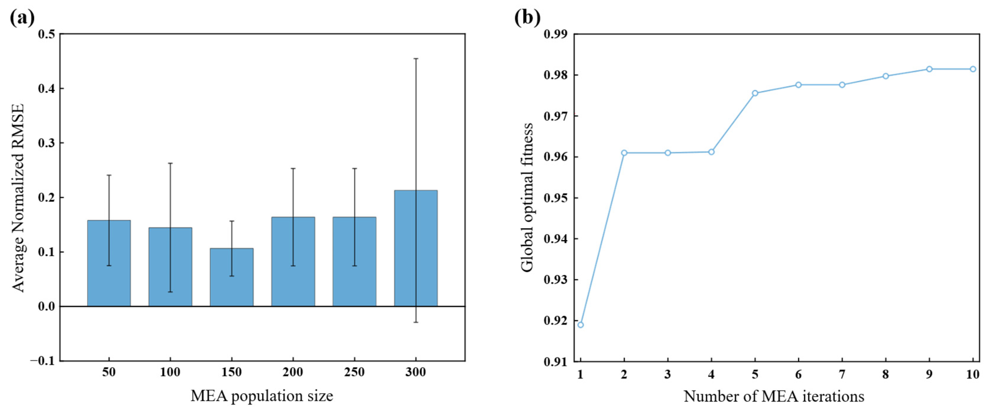
Individuals in the initial MEA population were randomly generated within predefined search bounds, and a fixed random seed was used to ensure the reproducibility of the optimization process. Each individual encoded all connection weights and bias parameters of the BP network. The optimal individual obtained through MEA search was decoded into the initial weights and biases of the BP network, which were subsequently fine-tuned using the Levenberg–Marquardt algorithm. To determine an appropriate MEA population-size range, comparative experiments were conducted using population sizes from 50 to 300 in increments of 50. As shown in Figure 16a, under a fixed BP network architecture, different MEA population sizes were compared through five-fold cross-validation within the development set. A population size of 150 produced the lowest mean normalized root mean square error. Further increases in population size did not lead to a sustained reduction in the mean error; in particular, the substantially increased inter-fold variability at a population size of 300 indicated that an excessively large population did not yield stable improvements in predictive performance. Therefore, the population size of the subsequent MEA-BP model was set to 150.
In summary, the parameter settings of the MEA-BP model are listed in Table 8. After determining these parameters, the convergence process of MEA-BP is shown in Figure 16b. As can be seen, the global best fitness increased rapidly during the early stage of MEA optimization, rising from 0.918 in the first iteration to 0.961 in the second iteration. Thereafter, the fitness increased gradually and stabilized after the ninth iteration, ultimately reaching 0.982. These results indicate that, under the selected population size and iteration settings, MEA can progressively optimize the initial weights and biases of the BP network and converge to a stable solution within the prescribed number of iterations.

4.4. Predictive-Performance Evaluation and Stability Validation of the Model

4.4.1. Comparative Analysis of Different Feature Encoding Methods

To evaluate the effect of explicitly preserving axial-order information on model predictive performance, the proposed seven-dimensional physically aggregated encoding was compared with the 48-dimensional order-preserving binary encoding described in Section 4.2. Both encoding methods were evaluated using the same dataset split, MEA-BP network architecture, optimization parameters, and pre-specified random initialization conditions to ensure a fair comparison. The comparison results are summarized in Table 9.
The results show that the seven-dimensional physically aggregated encoding achieved lower prediction errors and higher coefficients of determination for both volume-averaged temperature and average shear rate. Therefore, the seven-dimensional physically aggregated encoding was adopted as the input representation for subsequent model comparisons. It should be noted that this result does not negate the physical relevance of axial order in the extrusion process; rather, it indicates only that explicitly retaining the complete axial arrangement did not improve model prediction performance for the current dataset, selected output variables, and fixed model settings. The higher input dimensionality of the 48-dimensional representation may increase the complexity of the learning task at the current sample size, thereby weakening the model’s generalization ability.

4.4.2. Evaluation of Predictive Performance and Stability

To evaluate the relative effectiveness of the MEA optimization strategy, conventional BP [38], GA-BP [39], and PSO-BP [40] were selected as benchmark models. Conventional BP was used to represent the baseline predictive capability without population-based optimization, whereas GA and PSO represent two commonly used approaches for BP parameter optimization: an evolutionary search mechanism based on selection, crossover, and mutation, and a population-based search mechanism based on velocity–position updates, respectively. The key parameter configurations of the BP, GA-BP, and PSO-BP models are summarized in Table 10.
After the network architecture and relevant hyperparameters had been determined within the development set, 28 independent hold-out test samples that were not involved in model training or hyperparameter selection were used to evaluate the generalization performance of the BP, GA-BP, PSO-BP, and MEA-BP models. Model performance was compared using MAE, RMSE, and R2.
To ensure consistency among the quantitative metrics, prediction-comparison plots, residual plots, and parity plots, the first independent run obtained using a pre-specified random seed was designated as the primary run. Table 10 and Table 11 and Figure 17, Figure 18, Figure 19, Figure 20 and Figure 21 are all prepared based on the results of the primary run.
The predictive performance of the four models in the primary run is compared in Table 11. Overall, all four models were able to effectively predict the volume-averaged temperature and average shear rate; however, their prediction accuracy varied across the optimization strategies. For both prediction targets, MEA-BP achieved lower MAE and RMSE values together with a higher coefficient of determination, indicating favorable overall predictive performance in the primary run.
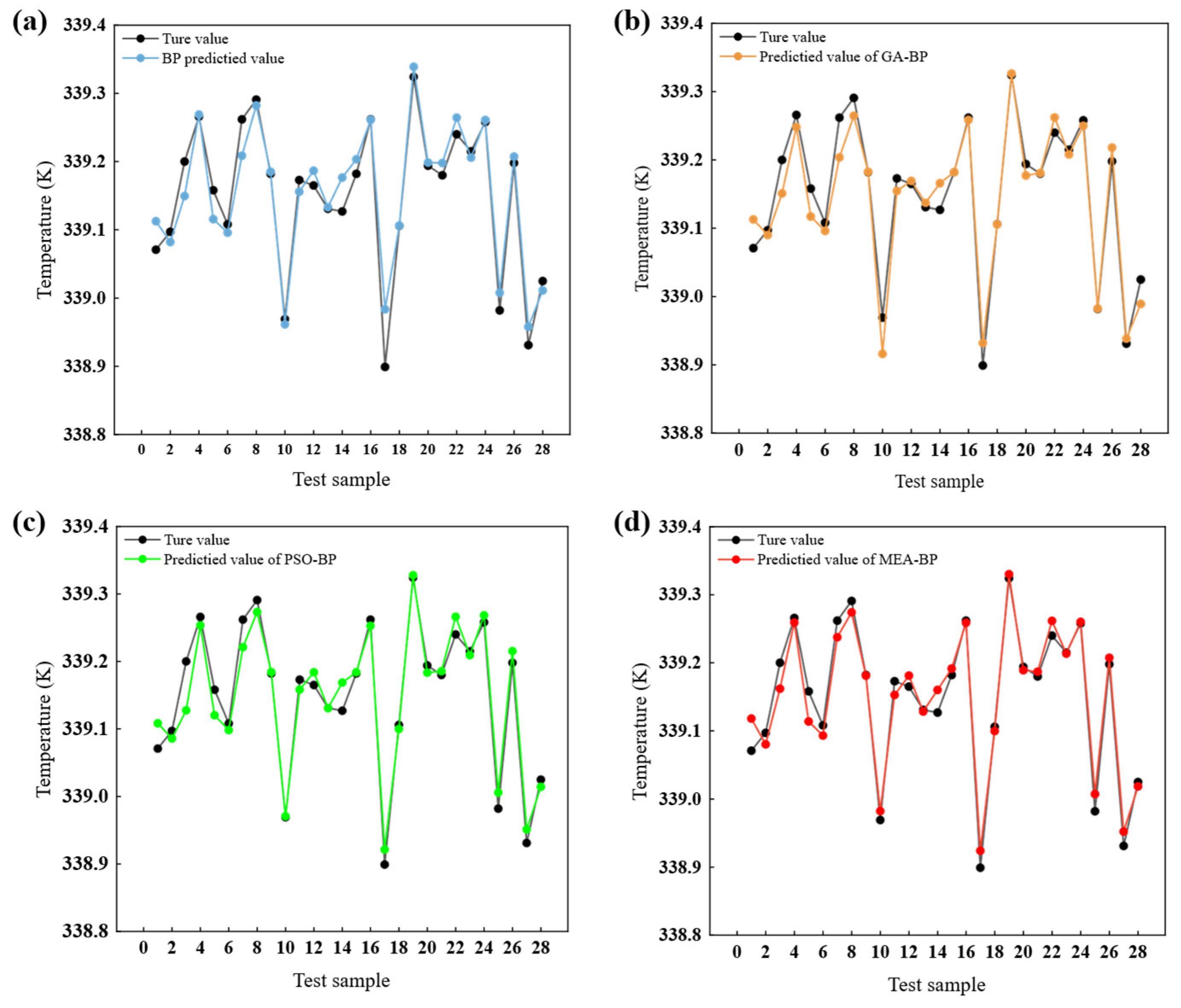
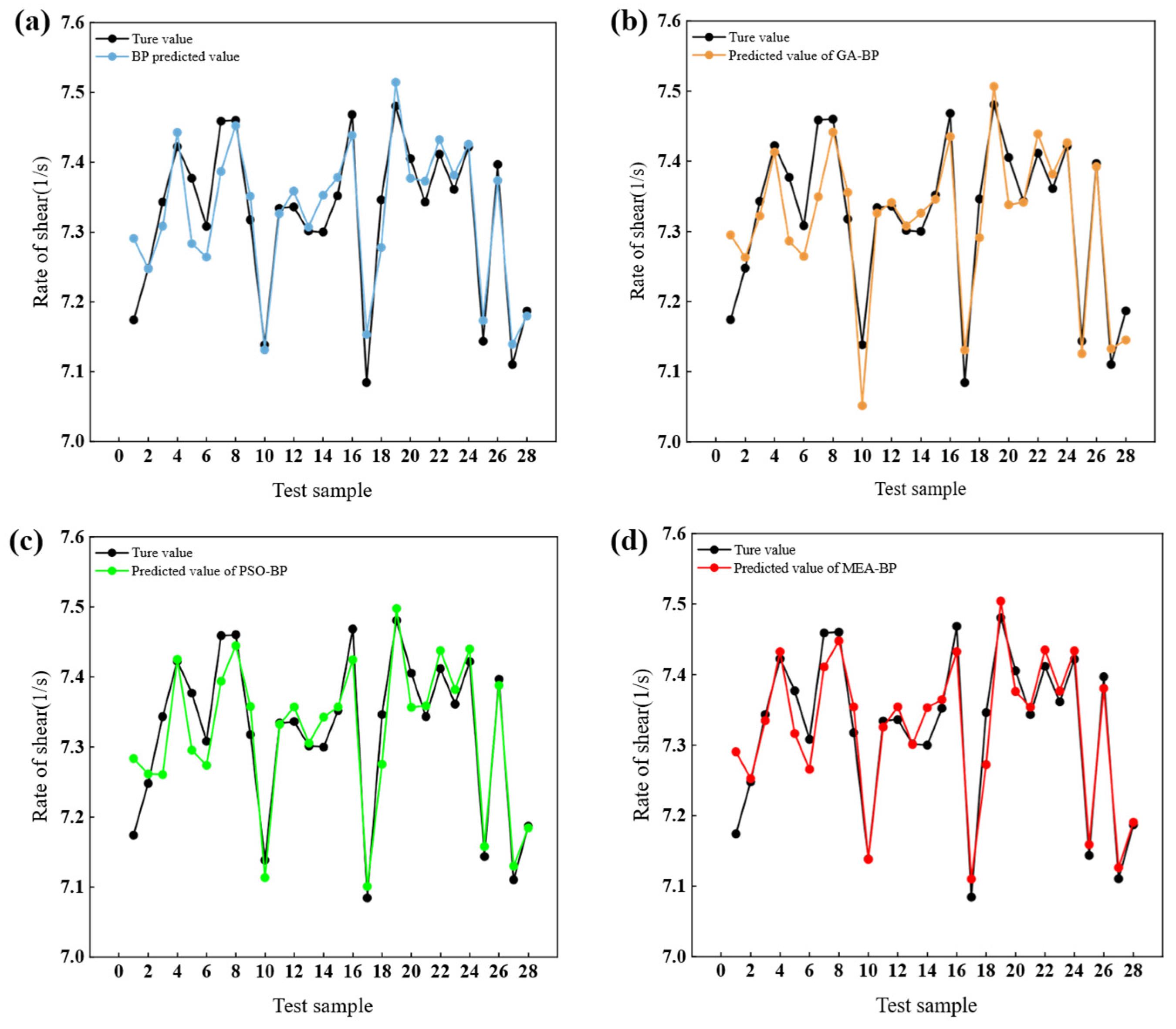
To further compare the ability of different models to capture the variation patterns of the independent test samples, Figure 17 and Figure 18 present comparisons between the predicted values of the four models and the finite element simulation results for volume-averaged temperature and average shear rate, respectively. The black curves represent the finite element simulation results, whereas the colored curves denote the predictions of the different models. As shown in the figures, all models captured the variation trends among the test samples to some extent, although deviations of varying magnitude remained near local peaks and valleys. By comparison, the predictions of the MEA-BP model were overall closer to the finite element simulation results.
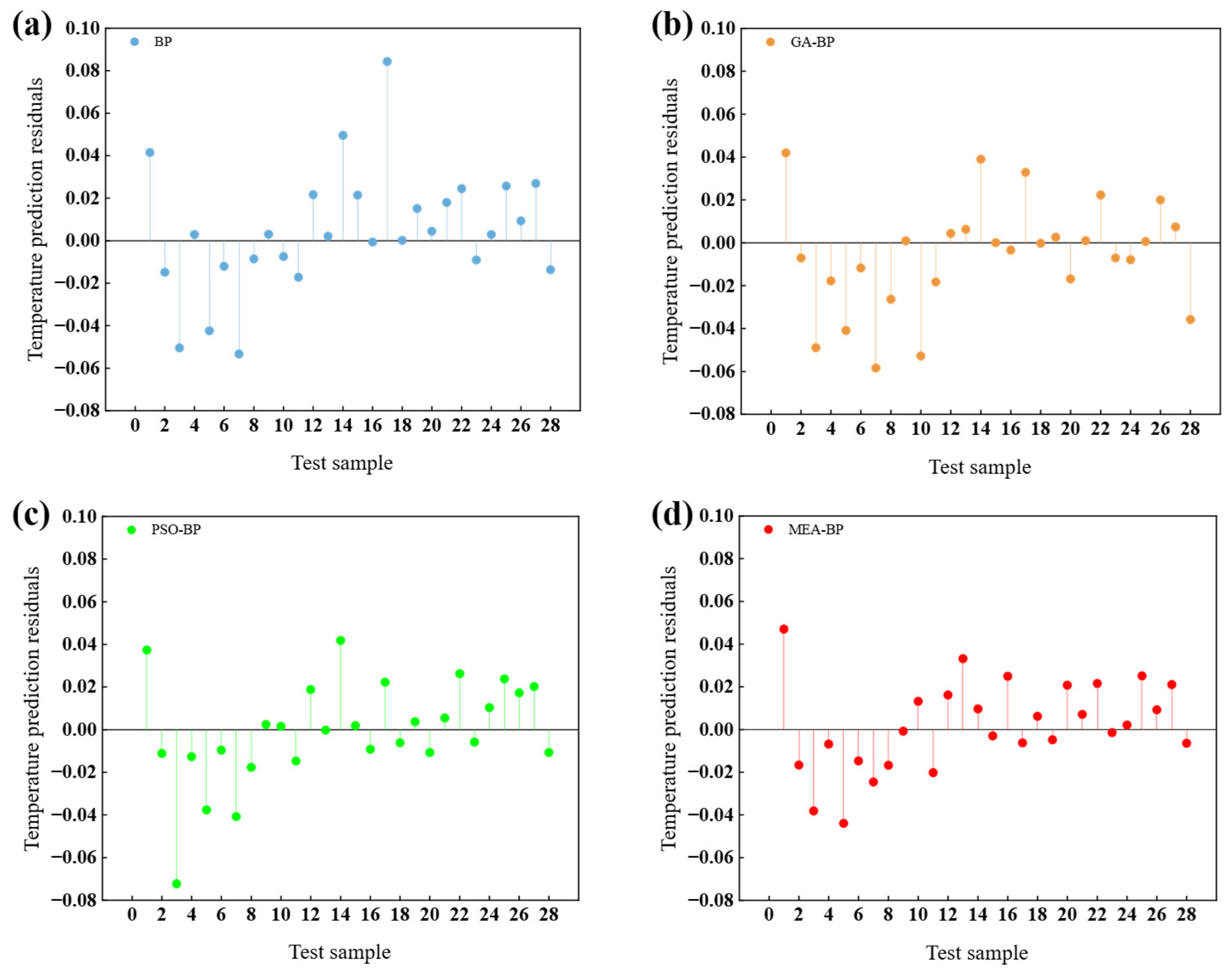
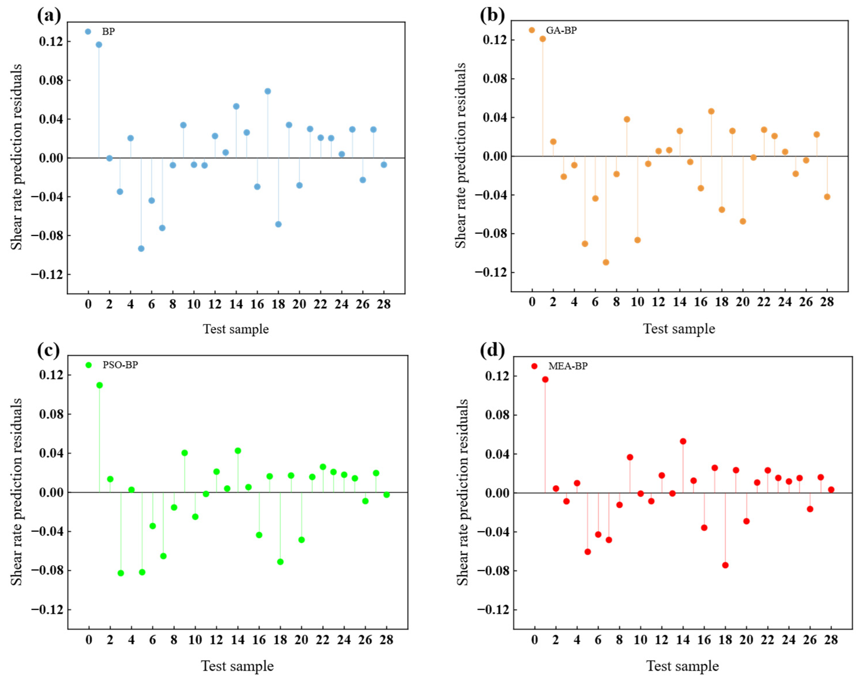
Figure 19 and Figure 20 further present the distributions of prediction residuals for the volume-averaged temperature and average shear rate obtained by the four models in the primary run. The residual is defined as the difference between the predicted value and the finite element simulation value, where positive and negative residuals indicate overprediction and underestimation of the corresponding output variable, respectively. Overall, the residuals of all models were mainly distributed around the zero line, although differences remained in the fluctuation range and local extreme values. For both prediction targets, the residuals of the MEA-BP model were more concentrated around the zero line, and relatively large positive and negative residuals occurred less frequently, which is consistent with the quantitative evaluation results in Table 10.
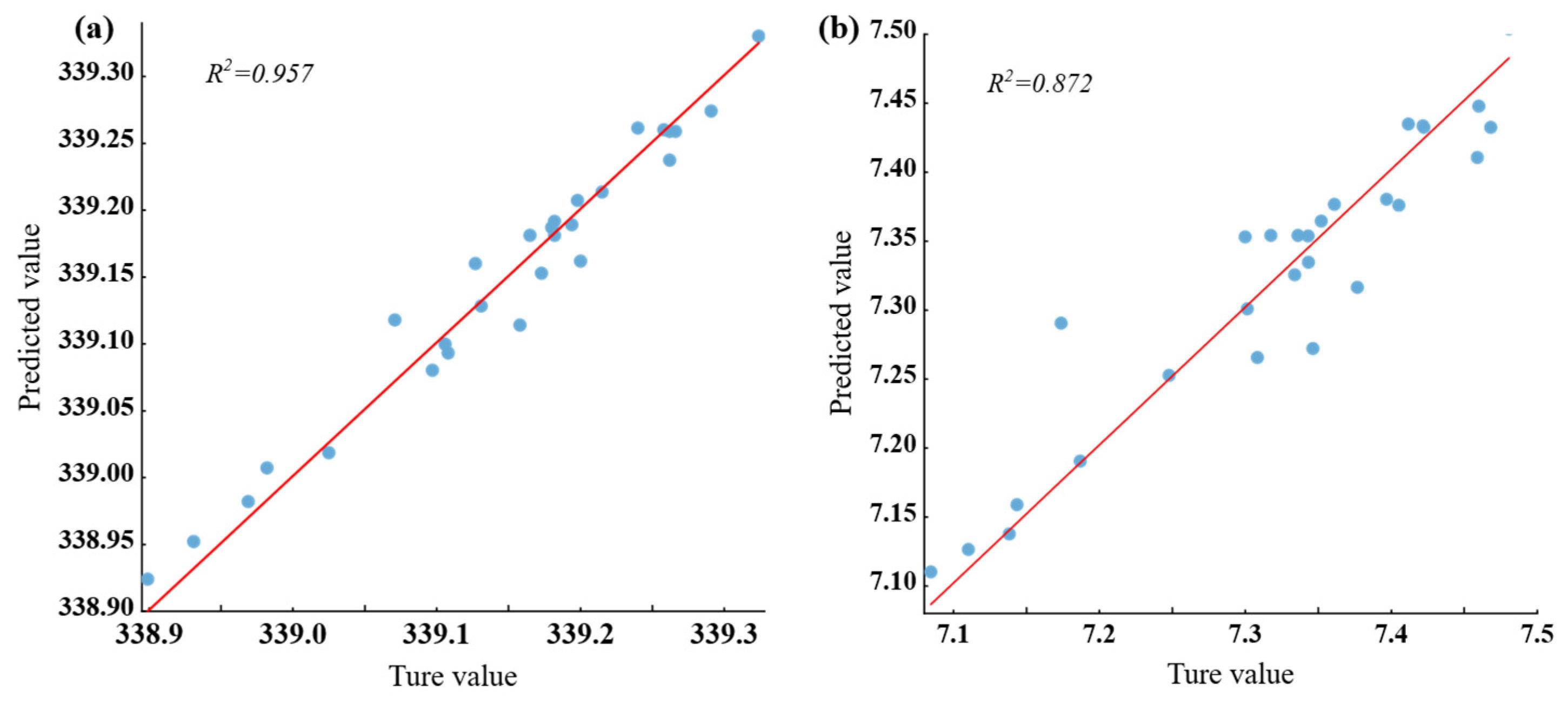
Based on the comparative results of the four models, parity plots were further used to verify the predictive consistency of the MEA-BP model. As shown in Figure 21, the red solid line represents the ideal parity line, y = x. Most test samples for the volume-averaged temperature and average shear rate are distributed near the ideal parity line, indicating that the MEA-BP model exhibits good predictive consistency for both target variables. Among them, the prediction points for volume-averaged temperature are more tightly concentrated around the parity line, whereas those for average shear rate are slightly more scattered, which may be related to the greater sensitivity of this variable to local flow conditions and variations in pin arrangement.
Considering the random initialization of the BP network and the stochastic nature of the GA, PSO, and MEA optimization processes, five pre-specified independent runs were conducted for each of the four models on the same independent test set. Table 12 reports the means and standard deviations of the repeated-run results, where the standard deviations characterize the sensitivity of the models to random initialization and optimization search paths. The repeated-run results indicate that MEA-BP maintained lower mean prediction errors and a higher mean coefficient of determination while exhibiting favorable overall run-to-run stability. Taken together, the sample-wise predictions, residual distributions, and parity plots from the pre-specified primary run, together with the repeated-run results, indicate that MEA-BP has favorable generalization performance and run-to-run stability on the dataset used in this study.
Given the distinct parameter-update mechanisms of BP, GA-BP, PSO-BP, and MEA-BP, wall-clock runtime was used as the common indicator of computational efficiency, rather than a single learning-rate-based comparison. All four models were evaluated using the same computational environment, finalized network settings, and data partition to ensure comparable runtime measurements. All four models were evaluated using the same computational environment, finalized network settings, and data partition to ensure comparable runtime measurements. Table 13 summarizes the mean wall-clock runtime and standard deviation of each model over five pre-defined independent executions.
The results show that, compared with conventional BP, population-intelligence optimization introduces additional computational overhead. The runtime of MEA-BP was numerically close to that of PSO-BP and did not show a lower runtime. However, under the current dataset size and fixed network architecture, all four models completed final training and prediction on the independent test set within 10 s. Therefore, the improved predictive performance of MEA-BP was achieved at a limited additional computational cost rather than through a computational-speed advantage.
From an engineering perspective, the volume-averaged melt temperature and average shear rate reflect the overall thermal state and mean deformation intensity of the melt during extrusion, respectively. Melt temperature affects material viscosity and flow behavior; excessively high temperatures may increase the risk of excessive shear heating and thermal degradation, whereas insufficient temperatures may hinder material plasticization and stable conveying. Average shear rate is related to the degree of melt deformation and viscous dissipation and can provide a reference for evaluating the relative effects of pin arrangements on flow intensification and shear heating. Therefore, improved prediction accuracy facilitates the rapid screening of candidate configurations that satisfy the desired temperature and shear-rate levels within the pin-arrangement design space and operating range defined in this study, reducing the need for high-fidelity finite element calculations for every case and providing a basis for prioritizing subsequent detailed numerical analyses or experimental validation.

5. Conclusions and Future Work

This study combined finite element simulations, preliminarily validated through comparison with measured temperatures and particle-tracing techniques, to investigate the effects of pin arrangements on rubber-melt mixing characteristics in a pin-barrel cold-feed extruder. A mind evolutionary algorithm-optimized BP neural network (MEA-BP) was further developed to rapidly predict the volume-averaged melt temperature and average shear rate. The results show that introducing pins enhanced shear heating and flow intensity, increased the overall melt temperature, and improved the cross-sectional temperature distribution. The pins also altered local flow states under laminar conditions, increased shear stress and the proportion of shear flow, and thereby promoted melt mixing. Particle-tracing results show that the pins promoted repeated splitting and merging of the fluid, thereby reducing particle agglomeration. Among the four uniform pin arrangements compared in this study, the configuration with four pins per group exhibited a faster reduction in the scale of segregation and a moderate residence time, providing a favorable balance between mixing adequacy and processing efficiency. This conclusion is limited to the four uniform pin arrangements compared in this study and does not imply that the four-pins-per-group configuration is globally optimal within a broader pin-arrangement design space.
Under consistent data partitioning, network settings, and evaluation protocols, MEA-BP exhibited lower mean prediction errors, higher mean coefficients of determination, and better run-to-run stability in predicting volume-averaged temperature and average shear rate. It should be noted that MEA-BP was developed only for the rapid prediction of two selected flow-field parameters and does not directly characterize or optimize overall mixing performance. This study was conducted primarily using finite element simulations, and experimental validation was limited to comparison of melt temperatures; direct experimental validation of mixing performance and systematic validation at an industrial production scale were not performed. In addition, the surrogate model was constructed using 140 numerical simulation cases, and its predictive capability mainly reflects its ability to fit and predict the corresponding simulation outputs. It is applicable to rapid numerical screening and trend assessment within the pin arrangements, geometry, EPDM material parameters, rheological model, boundary conditions, and operating range defined in this study. The reliability of extrapolative predictions beyond the current data range requires further validation.
Although the trained MEA-BP model can reduce the need for repeated finite element, the simulations, generation of the training data still relies on 140 three-dimensional non-isothermal finite element simulations. The current sample size represents a compromise between computational cost and the sampling requirements of the design space. Future work may expand the dataset to cover different geometries, material systems, and operating conditions, and incorporate experimental data on pressure, torque, and mixing performance for multi-metric validation. In addition, optimization methods such as RCGA, adaptive PSO, RCGA-PSO, and DE can be introduced for systematic comparison under consistent computational budgets and evaluation conditions. Time-resolved transient CFD, experimental, or industrial-process data can also be combined with temporal splitting or rolling-validation strategies to further assess model applicability, stability, and robustness in complex design spaces and time-varying operating conditions.

Author Contributions

Conceptualization, F.H. and H.Z.; methodology, H.Z.; software, H.Z.; validation, H.Z. and F.H.; formal analysis, H.Z. and X.Z.; investigation, F.H.; resources, F.H.; data curation, J.P.; writing—original draft preparation, H.Z.; writing—review and editing, J.P., J.Y. and X.Z.; visualization, H.Z.; supervision, J.P.; project administration, F.H.; funding acquisition, F.H. All authors have read and agreed to the published version of the manuscript.

Funding

This research was funded by Guangxi Key Research and Development Program Project Grant No. AB24010202.

Institutional Review Board Statement

Not applicable.

Informed Consent Statement

Not applicable.

Data Availability Statement

The original contributions presented in this study are included in the article. Additional data are available from the corresponding author upon reasonable request.

Conflicts of Interest

The authors declare no conflicts of interest.

References

  1. Saputra, R.; Walvekar, R.; Khalid, M.; Mubarak, N.M.; Sillanpää, M. Current progress in waste tire rubber devulcanization. Chemosphere 2021, 265, 129033. [Google Scholar] [CrossRef] [PubMed]
  2. Bigio, D.; Young, D. The effect of fluid decoupling on viscous mixing. Polym. Eng. Sci. 1993, 33, 1270–1278. [Google Scholar] [CrossRef]
  3. Rauwendaal, C. (Ed.) Mixing in Polymer Processing; M. Dekker: New York, NY, USA, 1991. [Google Scholar]
  4. Yao, W.G.; Takahashi, K.; Koyama, K.; Dai, G.C. Design of a new type of pin mixing section for a screw extruder based on analysis of flow and distributive mixing performance. Chem. Eng. Sci. 1997, 52, 13–21. [Google Scholar] [CrossRef]
  5. Yabushita, Y.; Brzoskowski, R.; White, J.L.; Najakima, N. Flow of rubber compound in a pin barrel screw extruder. Int. Polym. Process. 1989, 4, 219–224. [Google Scholar] [CrossRef]
  6. Shin, K.-C.; White, J.L. Basic studies of extrusion of rubber compounds in a pin barrel extruder. Rubber Chem. Technol. 1993, 66, 121–138. [Google Scholar] [CrossRef]
  7. Brzoskowski, R.; White, J.L.; Szydlowski, W.; Nakajima, N.; Min, K. Modelling flow in pin-barrel screw extruders. Int. Polym. Process. 1988, 3, 134–140. [Google Scholar] [CrossRef]
  8. Schöppner, V.; Schadomsky, M.; Hopmann, C.; Lemke, F. Investigations of the mixing behaviour of pin-type rubber extruders. AIP Conf. Proc. 2016, 1713, 130003. [Google Scholar] [CrossRef]
  9. Wang, Z.; Pan, Y.; Liu, Y.; Huang, J.; Wang, N.; Hu, X. Investigations of the elongational deformation induced by pins in pin-barrel cold-feed extruders. Adv. Polym. Technol. 2022, 2022, 3513804. [Google Scholar] [CrossRef]
  10. Yao, W.G.; Tanifuji, S.; Takahashi, K.; Koyama, K. Mixing efficiency in a pin mixing section for single-screw extruders. Polym. Eng. Sci. 2001, 41, 908–917. [Google Scholar] [CrossRef]
  11. Zhou, H.; Zhang, J.; Lim, S.E.; Ferraris, E.; Le Ferrand, H. Rationalising the onset of bistability in polylactic acid (PLA) bilayer laminates using fused filament fabrication (FFF). Virtual Phys. Prototyp. 2026, 21, e2618395. [Google Scholar] [CrossRef]
  12. Lubura, J.D.; Kojić, P.; Pavličević, J.; Ikonić, B.; Omorjan, R.; Bera, O. Prediction of rubber vulcanization using an artificial neural network. Hem. Ind. 2021, 75, 277–283. [Google Scholar] [CrossRef]
  13. Uruk, Z.; Kiraz, A. Artificial intelligence based prediction models for rubber compounds. J. Polym. Eng. 2023, 43, 113–124. [Google Scholar] [CrossRef]
  14. Yuan, Z.; Niu, M.-Q.; Ma, H.; Gao, T.; Zang, J.; Zhang, Y.; Chen, L.-Q. Predicting mechanical behaviors of rubber materials with artificial neural networks. Int. J. Mech. Sci. 2023, 249, 108265. [Google Scholar] [CrossRef]
  15. Robin, E.; Le Cam, J.-B.; Delahaye, G.; Ruellan, B.; Di Cesare, N.; Canévet, F. A first proposal for fatigue life prediction of carbon black filled natural rubber at different temperatures with an artificial neural network. Strain 2025, 61, e70001. [Google Scholar] [CrossRef]
  16. Sui, C.; Qiao, D.; Wu, Y.; Zhu, H.; Lan, H.; Yang, W.; Guo, Q. Study of the effect of retarder and expander on the strength and cracking performance of rubber concrete based on back propagation neural network. Materials 2023, 16, 6976. [Google Scholar] [CrossRef] [PubMed]
  17. Hou, H.-L.; Zhang, G.-P.; Chen, X.; Zhao, Y.-Q. Quality prediction of internal thread cold extrusion based on genetic algorithm optimized BP neural network. Adv. Mech. Eng. 2022, 14, 16878132221089148. [Google Scholar] [CrossRef]
  18. Xiang, K.-L.; Xiang, P.-Y.; Wu, Y.-P. Prediction of the fatigue life of natural rubber composites by artificial neural network approaches. Mater. Des. 2014, 57, 180–185. [Google Scholar] [CrossRef]
  19. Beklaryan, G.L.; Akopov, A.S.; Khachatryan, N.K. Optimisation of system dynamics models using a real-coded genetic algorithm with fuzzy control. Cybern. Inf. Technol. 2019, 19, 87–103. [Google Scholar] [CrossRef]
  20. Peng, Z.; Wu, L.; Chen, Z. NHL and RCGA based multi-relational fuzzy cognitive map modeling for complex systems. Appl. Sci. 2015, 5, 1399–1411. [Google Scholar] [CrossRef]
  21. Al-Itry, R.; Lamnawar, K.; Maazouz, A. Improvement of thermal stability, rheological and mechanical properties of PLA, PBAT and their blends by reactive extrusion with functionalized epoxy. Polym. Degrad. Stab. 2012, 97, 1898–1914. [Google Scholar] [CrossRef]
  22. Sun, Y.; Wang, S.; Huang, S.; Pan, W.; He, Y.; Jian, R. Mixing and thermal transport behavior in a pin or non-pin extruder equipped with a field synergy elongation screw. Polymers 2024, 16, 1793. [Google Scholar] [CrossRef] [PubMed]
  23. Pan, W.; Wang, S.; Huang, T.; Jiang, X.; Jian, R. Effect of screw design on the mixing and heat efficiencies in an extrusion system by tailoring ductile forming with field synergy principle. Appl. Therm. Eng. 2025, 262, 125291. [Google Scholar] [CrossRef]
  24. Sun, C.; Sun, Y.; Wei, L. Mind-evolution-based machine learning: Framework and the implementation of optimization. In Proceedings of the IEEE International Conference on Intelligent Engineering Systems (INES’98), Vienna, Austria, 17–19 September 1998; pp. 355–359. [Google Scholar]
  25. Guha, S.; Jana, R.K.; Sanyal, M.K. Artificial neural network approaches for disaster management: A literature review. Int. J. Disaster Risk Reduct. 2022, 81, 103276. [Google Scholar] [CrossRef]
  26. Zhang, Y.; Wang, X.; Zhang, J.; Chen, X.; Wu, H.; Chen, Y. Research on slope excavation stability based on PSO-BP reinforcement optimization algorithm. Appl. Sci. 2025, 15, 11726. [Google Scholar] [CrossRef]
  27. Xu, T.; Huang, J.; Li, Y.; Chen, T. Predicting ceramic wool diameter by motor frequency using improved BP neural network. Appl. Sci. 2023, 13, 226. [Google Scholar] [CrossRef]
  28. Guo, Y.; Zhao, Z.; Huang, L. SoC estimation of lithium battery based on improved BP neural network. Energy Procedia 2017, 105, 4153–4158. [Google Scholar] [CrossRef]
  29. Goh, A.T.C. Back-propagation neural networks for modeling complex systems. Artif. Intell. Eng. 1995, 9, 143–151. [Google Scholar] [CrossRef]
  30. Wang, H.; Li, S.; Zhen, S.; Liu, J.; Peng, X.; Yi, Y. Study of peak velocity of blasting vibration for raft foundation demolition based on MEA-BP algorithm. AIP Adv. 2024, 14, 085129. [Google Scholar] [CrossRef]
  31. Nan, J.; Zheng, J.; Jiang, B.; Li, Y.; Chen, J.; Fan, X. A multi-objective optimization design method for high-aspect-ratio wing structures based on mind evolution algorithm backpropagation surrogate model. Machines 2024, 12, 907. [Google Scholar] [CrossRef]
  32. Zhang, J.; Li, P.; Yin, X.; Wang, S.; Zhu, Y. Back analysis of surrounding rock parameters in Pingdingshan mine based on BP neural network integrated mind evolutionary algorithm. Mathematics 2022, 10, 1746. [Google Scholar] [CrossRef]
  33. Pinni, K.S.; Chandy, A.J. Investigation of non-isothermal effects in differential viscoelastic simulations of industrial-scale rubber extrusion. J. Non-Newton. Fluid Mech. 2026, 349, 105608. [Google Scholar] [CrossRef]
  34. Shields, M.D.; Zhang, J. The generalization of Latin hypercube sampling. Reliab. Eng. Syst. Saf. 2016, 148, 96–108. [Google Scholar] [CrossRef]
  35. Rodríguez, P.; Bautista, M.A.; Gonzàlez, J.; Escalera, S. Beyond one-hot encoding: Lower dimensional target embedding. Image Vis. Comput. 2018, 75, 21–31. [Google Scholar] [CrossRef]
  36. Wang, F.; Tian, D.; Lowe, L.; Kalin, L.; Lehrter, J. Deep learning for daily precipitation and temperature downscaling. Water Resour. Res. 2021, 57, e2020WR029308. [Google Scholar] [CrossRef]
  37. Pan, Y.; Wang, Y.; Zhou, P.; Yan, Y.; Guo, D. Activation functions selection for BP neural network model of ground surface roughness. J. Intell. Manuf. 2020, 31, 1825–1836. [Google Scholar] [CrossRef]
  38. Zhang, J.-R.; Zhang, J.; Lok, T.-M.; Lyu, M.R. A hybrid particle swarm optimization–back–propagation algorithm for feedforward neural network training. Appl. Math. Comput. 2007, 185, 1026–1037. [Google Scholar] [CrossRef]
  39. Zheng, D.; Qian, Z.; Liu, Y.; Liu, C. Prediction and sensitivity analysis of long-term skid resistance of epoxy asphalt mixture based on GA-BP neural network. Constr. Build. Mater. 2018, 158, 614–623. [Google Scholar] [CrossRef]
  40. Møller, M.F. A scaled conjugate gradient algorithm for fast supervised learning. Neural Netw. 1993, 6, 525–533. [Google Scholar] [CrossRef]
Figure 1. Research method and workflow.
Applsci 16 06880 g001
Figure 2. Experimental platform and simulation model: (a) experimental platform; (b) pin-barrel section; (c) fluid-domain models with different pin arrangements; (d) simulation model and boundary conditions.
Applsci 16 06880 g002
Figure 3. MST-based mesh superposition.
Applsci 16 06880 g003
Figure 4. Velocity streamline plots in the channel under different pin numbers.
Applsci 16 06880 g004
Figure 5. Cross-sectional temperature under different pin numbers.
Applsci 16 06880 g005
Figure 6. Mixing characteristics under different numbers of pins: (a) mixing-index distribution; (b) maximum shear-stress curves.
Applsci 16 06880 g006
Figure 7. Probability distribution of maximum shear stress under different pin numbers: (a) 0 pins; (b) 2 pins; (c) 4 pins; (d) 6 pins.
Applsci 16 06880 g007
Figure 8. Distributive mixing and residence-time characteristics under different numbers of pins: (a) scale of segregation; (b) cumulative residence-time curves.
Applsci 16 06880 g008
Figure 9. Probability distribution of cumulative residence time under different pin numbers: (a) 0 pins; (b) 2 pins; (c) 4 pins; (d) 6 pins.
Applsci 16 06880 g009
Figure 10. Spatial distributions of tracer particles under different pin-number configurations.
Applsci 16 06880 g010
Figure 11. Evolutionary workflow of MEA.
Applsci 16 06880 g011
Figure 12. Topology of the BP neural network.
Applsci 16 06880 g012
Figure 13. Training workflow of the MEA-BP neural network model.
Applsci 16 06880 g013
Figure 14. Model development workflow incorporating five-fold cross-validation within the development set and evaluation using an independent hold-out test set.
Applsci 16 06880 g014
Figure 15. Hyperparameter optimization of the BP neural network: (a) comparison of activation functions; (b) comparison of the number of hidden-layer nodes.
Applsci 16 06880 g015
Figure 16. MEA population size and convergence curve: (a) comparison of different population sizes; (b) convergence curve.
Applsci 16 06880 g016
Figure 17. Comparison between the predicted and simulated volume-averaged temperatures of the four models on the independent test set: (a) BP; (b) GA-BP; (c) PSO-BP; (d) MEA-BP.
Applsci 16 06880 g017
Figure 18. Comparison between the predicted and simulated values of average shear rate for the four models on the independent test set: (a) BP; (b) GA-BP; (c) PSO-BP; (d) MEA-BP.
Applsci 16 06880 g018
Figure 19. Distribution of prediction residuals for volume-averaged temperature obtained by the four models on the independent test set: (a) BP; (b) GA-BP; (c) PSO-BP; (d) MEA-BP.
Applsci 16 06880 g019
Figure 20. Distribution of prediction residuals for average shear rate obtained by the four models on the independent test set: (a) BP; (b) GA-BP; (c) PSO-BP; (d) MEA-BP.
Applsci 16 06880 g020
Figure 21. Parity plots of the predicted and simulated values of the model on the independent test set: (a) volume-averaged temperature; (b) average shear rate.
Applsci 16 06880 g021
Table 1. Material properties of EPDM used in the simulation.
ParameterSymbolValue
Densityρ1130 kg·m−3
Specific heat capacityCp1700 J·kg−1·K−1
Thermal conductivityk0.18 W·m−1·K−1
Viscosity at an infinite shear rateη0 Pa·s
Zero shear viscosityη0178,800 Pa·s
Nature timeλ10.8 s
Non-Newtonian indexn0.4
Coefficient of temperature sensibilityα0.0025 K−1
Reference temperatureTα332.87 K
Table 2. Boundary conditions.
BoundaryFlow ConditionsThermal Conditions
InletFully developed, volumetric flow rate 2.04 × 10⁻⁶ m3·s−1332.87 K
OutletFlow outflowHeat outflow
Barrel wallStationary, no-slip wall335.52 K
Screw wallScrew speed 30 r·min−1Insulated boundary
Table 3. Mesh independence verification of the fluid model.
Grid QualityNumber of Mesh Elements, (×105)Shear Rate (s−1)Average Temperature (K)
Coarse2.57.79339.3
Medium3.57.87339.4
Fine4.57.96338.9
Table 4. Comparison of simulated and measured melt temperatures at different screw speeds.
Screw Speed (r/min)Simulation Data (K)Experimental Data (K)Difference (%)
20337.99337.341.01
30339.49339.870.57
40341.36342.111.08
Table 5. Pin distribution patterns.
ModeNumber of PinsAngular Position (°)Distribution Feature
10-No empty
21Single pin
31180°Single pin
420°, 180°Two pins
5260°, 240°Two pins
62120°, 300°Two pins
730°, 120°, 240°Three pins
8360°, 180°, 300°Three pins
940°, 60°, 180°, 240°Four pins
1040°, 120°, 180°, 300°Four pins
11460°, 120°, 240°, 300°Four pins
12560°, 120°, 180°, 240°, 300°Five pins
1350°, 60°, 120°, 240°, 300°Five pins
1460°, 60°, 120°, 180°, 240°, 300°Full pins
Table 6. Simulation experimental data.
Serial NumberPin Group CategoryFlow Field Data
FirstSecondThirdFourthFifthSixthSeventhEighthTemperature (K)Shear Rate (s−1)
1121412949124339.2847.43221
211241311106338.9266.99939
339131811148339.1617.26317
….
1382983613138339.1517.30278
1392268142113339.0257.18691
140105553141114339.2297.40599
Table 7. Data after aggregated feature transformation.
Samplex1x2x3x4x5x6x7Temperature (K)Shear Rate (s−1)
122212110339.2847.43221
232222112338.9266.99939
322221110339.1617.26317
13833211212339.1517.30278
13922221110339.0257.18691
14033222214339.2297.40599
Table 8. Parameter settings of MEA-BP.
Population SizeNumber of Winning SubpopulationsNumber of Temporary SubpopulationsSubpopulation SizeNumber of Input NodesNumber of Hidden NodesNumber of Output NodesNumber of Iterations
150552074210
Table 9. Comparison of two feature encoding methods in the MEA-BP model.
Encoding MethodInput
Dimension
Temperature MAE (×10−2)Temperature RMSE (×10−2)Temperature R2Shear-Rate MAE (×10−2)Shear-Rate RMSE (×10−2)Shear-Rate R2
Physically
aggregated
71.742.230.9572.893.990.872
Sequence preserving binary484.285.610.5834.736.760.535
Table 10. Key training and optimization parameter settings for the BP, GA-BP, and PSO-BP models.
ModelParametersNumerical/Method
BPTraining algorithmtrainlm
Parameter optimizationRandom initialization
Maximum training times150
Performance objective1 × 10−4
GA-BPPopulation size40
Maximum number of iterations20
Search scope[−3, 3]
Cross probability0.3
Mutation probability0.5
PSO-BPParticle swarm size60
Maximum number of iterations20
Inertia weight0.6
Learning factorc1 = 2, c2 = 2
Position/Speed Boundary[−3, 3]
Table 11. Comparison of the predictive performance of the four models.
ModelPrediction TargetMAE (×10−2)RMSE (×10−2)R2
BPTemperature2.092.880.926
Shear rate3.354.340845
GA-BPTemperature1.902.600.941
Shear rate3.484.740.818
PSO-BPTemperature1.762.370.950
Shear rate3.104.150.861
MEA-BPTemperature1.742.230.957
Shear rate2.893.990.872
Table 12. Comparison of repeated-run performance and stability among the four models.
ModelPrediction TargetMAE (×10−2)RMSE (×10−2)R2
BPTemperature2.11 ± 0.152.91 ± 0.260.916 ± 0.012
Shear rate3.41 ± 0.224.38 ± 0.340.837 ± 0.024
GA-BPTemperature1.88 ± 0.042.53 ± 0.080.944 ± 0.028
Shear rate3.39 ± 0.204.56 ± 0.420.830 ± 0.031
PSO-BPTemperature1.97 ± 0.302.97 ± 0.810.921 ± 0.043
Shear rate3.66 ± 0.715.51 ± 1.760.734 ± 0.166
MEA-BPTemperature1.75 ± 0.092.28 ± 0.110.954 ± 0.005
Shear rate2.98 ± 0.204.11 ± 0.260.863 ± 0.018
Note: All results reported in the table were obtained using the same independent test set.
Table 13. Running times of the four models over five runs.
ModelNumber of Independent RunsAverage Time (s)Standard Deviation (s)
BP55.30.9
GA-BP56.30.6
PSO-BP58.70.3
MEA-BP58.80.8
Note: The timing scope included network training and prediction on the independent test set.
Disclaimer/Publisher’s Note: The statements, opinions and data contained in all publications are solely those of the individual author(s) and contributor(s) and not of MDPI and/or the editor(s). MDPI and/or the editor(s) disclaim responsibility for any injury to people or property resulting from any ideas, methods, instructions or products referred to in the content.