Experimental Physics-Motivated Residual Learning for Steam-Assisted High-Viscosity Oil Production and Thermal-Efficiency-Based Steam-Supply Selection

Abstract

Steam injection is an energy-intensive enhanced-oil-recovery method for high-viscosity reservoirs, and its performance is controlled by coupled heat delivery, steam condensation, temperature-dependent viscosity reduction, mobility change and reservoir filtration response. This study develops an experimentally validated physics-motivated residual-learning framework for forecasting oil production and selecting thermally rational steam-supply regimes. The model combines a physics-motivated semi-empirical baseline describing useful steam-related heat input, calibrated viscosity transformation, mobility growth, steam–oil ratio and a thermal-energy efficiency index with a residual-learning block fitted to measured regime-level records. The supervised forecasting task was performed at the regime level using 200 operating-regime records treated as the effective modelling units, with nested logs aggregated within regimes and within-group dependence examined through campaign-, reservoir-state- and well-availability-based checks. The 4800 steam-injection log entries and 4800 production-response log entries were treated as nested time-resolved measurements used only for regime-level aggregation, feature construction and quality-control checks; they were not counted as independent training samples. Blind-test validation produced R² values of 0.974 for oil rate, 0.988 for cumulative oil production, 0.731 for steam–oil ratio and 0.828 for the thermal-energy efficiency index; the corresponding MAPE values were 4.56%, 3.86%, 4.48% and 3.29%, respectively. The error structure shows higher uncertainty for composite indicators than for direct production responses, which is consistent with the measurement chain. Response-surface and Pareto analyses identify bounded steam-supply operating regions where production gain remains balanced against specific steam consumption and the thermal-energy efficiency index.

1. Introduction

High-viscosity oil and natural bitumen reservoirs require a simultaneous increase in production mobility and control of the energy penalty associated with thermal stimulation [1]. Steam injection remains one of the most widely applied thermal enhanced-oil-recovery methods because latent heat release and reservoir heating can sharply reduce oil viscosity [2,3,4]. The production response, however, is governed by a coupled set of processes: heat transfer along the well-reservoir system, partial steam condensation, saturation redistribution, temperature-dependent viscosity reduction, relative-permeability change and the formation of a spatially nonuniform high-mobility zone. These coupled mechanisms make production forecasting nonlinear, regime-dependent and sensitive to both reservoir properties and steam-operation variables [5].

The engineering difficulty lies in the fact that increasing steam rate does not automatically increase useful oil recovery. When steam quality, formation depth, permeability, initial viscosity or exposure duration are unfavourable, additional heat input may mainly increase heat losses and the steam–oil ratio rather than production [6]. Rational steam-supply selection therefore requires models that forecast the production response, quantify the energy consequence of the regime and preserve the physical link between heat delivery, viscosity reduction and filtration response [7].

Empirical correlations are useful for screening, but they are usually restricted to the calibration domain and cannot reliably represent interacting effects of steam quality, temperature, reservoir conductivity and oil rheology. High-fidelity thermal reservoir simulation offers stronger physics, yet it is computationally expensive and inconvenient for rapid multi-regime operating-window assessment. Purely data-driven models may capture nonlinearities, but without explicit physical structure they can learn non-transferable associations between steam-operation variables and production indicators [8]. A hybrid residual-learning architecture is therefore appropriate: the baseline represents the primary thermal and filtration mechanisms, while the learning block corrects measured residuals that remain after the physical baseline has been evaluated.

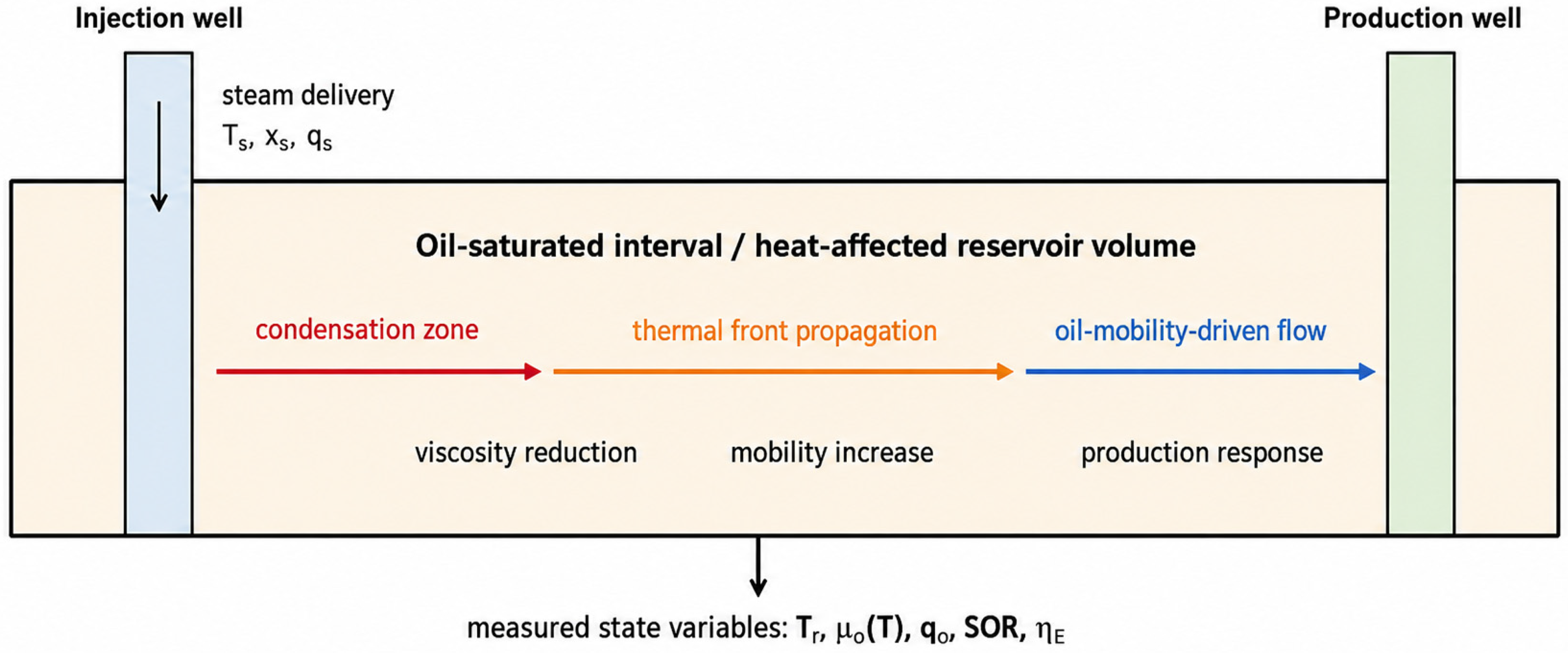
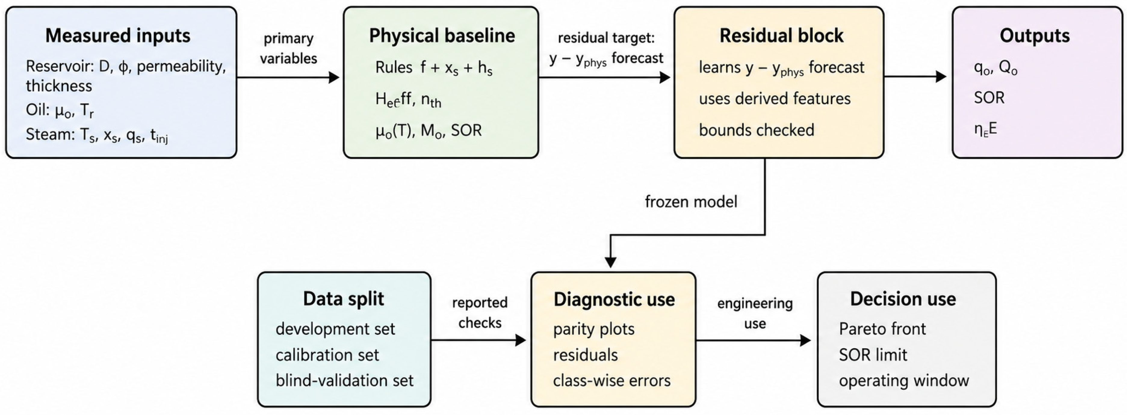
The structure of the proposed approach is shown in Figure 1. The workflow separates measured reservoir and steam-operation variables from the physics-motivated semi-empirical baseline and the residual-learning correction. This separation is essential because steam rate, steam quality and exposure duration do not act on production directly; they first determine useful heat delivery, calibrated viscosity reduction and mobility growth, which then form the production response, SOR and thermal-energy efficiency indicators [9,10,11].

The architecture avoids direct black-box mapping from steam-injection variables to production indicators. Reservoir and steam-operation records first enter the physics-motivated semi-empirical baseline, where useful heat input, calibrated viscosity reduction, oil mobility and steam–oil ratio are estimated from interpretable engineering relations. The trainable component is then restricted to the residual part of the response, which increases flexibility while preserving the main heat–viscosity–mobility logic of the thermal process.

The information basis of the work is a measured dataset of steam–thermal exposure regimes. Regime-level records, steam-operation logs and production-response logs are linked by experiment identifiers, and the validation subset is excluded from physical-parameter identification, residual-model training and hyperparameter selection. This design limits data leakage and makes the reported forecast quality interpretable as a prediction on previously unused operating regimes, while grouped checks are used to quantify the possible effect of campaign-, reservoir-state- and well-related dependence.

The scientific novelty of the study is threefold. First, high-viscosity-oil production forecasting is formulated as a residual-learning problem structured by useful heat delivery, calibrated viscosity transformation, oil mobility and steam consumption. Second, the model uses physically interpretable derived features rather than unrestricted empirical predictors. Third, steam-supply optimization is formulated as an operating-window problem in which production gain, SOR and the thermal-energy efficiency index are considered jointly.

The aim of the work is to develop an experimentally validated physics-motivated residual-learning framework for forecasting high-viscosity-oil production under steam injection and to determine rational steam-supply regimes under production, SOR and thermal-energy efficiency constraints. The tasks are: to define the physically interpretable input space; to construct derived heat-transfer and mobility features; to train the residual-learning correction without leakage from validation records; to evaluate prediction accuracy and residual structure; and to identify a steam-supply operating window using production, SOR and energy-efficiency criteria.

The paper is organized as follows. Section 2 describes the physical process setting and the dominant mechanisms of steam-thermal exposure. Section 3 specifies the experimental data structure and validation logic. Section 4 presents the hybrid forecasting model. Section 5 formulates steam-supply optimization. Section 6 and Section 7 report prediction, interpretation and validation results, followed by discussion and conclusions.

2. Physical Process Setting and Conceptual Model of Steam-Thermal Exposure

Forecasting production under steam injection requires an explicit causal chain: steam supply → heat delivery to the reservoir → reduction in oil viscosity → mobility increase and filtration response → production and energy-efficiency indicators. Figure 2 presents this chain as a control-volume interpretation rather than as a decorative workflow.

The control-volume structure of the dominant thermal and filtration mechanisms is shown in Figure 2.

The physical response is governed by useful heat delivered to the oil-saturated interval, not by nominal steam rate alone. Heat losses, steam quality, depth, reservoir conductivity and temperature-dependent viscosity determine whether the injected heat is converted into mobility growth or dissipated without proportional production gain. This interpretation defines the variables retained in the baseline model and the constraints used during optimization.

2.1. Thermodynamic and Filtration Essence of the Process

Steam-thermal action on the reservoir of high-viscosity oil is a conjugate process of transfer of energy, mass and momentum in an inhomogeneous porous medium [12]. After steam is supplied, part of the thermal energy is spent on heat losses in the wellbore and in the downhole zone, and the remaining part enters the reservoir, where it initiates heating of the skeleton of the porous medium, produced water and oil [13,14]. At the same time, depending on the pressure, temperature, dryness of the steam and thermal properties of the formation, partial or intensive condensation of the vapour phase occurs, accompanied by the release of latent heat. It is this mechanism that is one of the most important sources of the local thermal effect [15,16].

In a first approximation, the effective heat flux actually involved in the reservoir process can be written as

$$Q_{\mathrm{eff}}={\dot{m}}_{\mathrm{steam}}{h}_{\mathrm{steam}}{\eta }_{\mathrm{th}},$$

where Qeff is the useful thermal power transferred to the reservoir; ṁsteam is the mass steam-flow rate; hsteam is the specific enthalpy of the injected steam; and ηth is the heat-delivery efficiency, which accounts for wellbore and near-wellbore losses. For wet steam, hsteam should be evaluated from the liquid-water enthalpy and the latent heat contribution determined by steam quality [17,18].

For production forecasting, the decisive quantity is not the nominal steam rate but the useful heat actually delivered to the oil-bearing interval. The same steam rate can produce different thermal responses when steam quality, temperature, reservoir depth, injection duration and heat-loss conditions differ. Therefore, steam-operation variables are treated as energy carriers with explicit thermophysical meaning rather than as formal regressors.

The key effect of heating is a sharp decrease in the viscosity of high-viscosity oil. For thermal production methods, this is a fundamental mechanism, since it is the reduction in viscosity that leads to an increase in mobility and facilitation of oil filtration to the production well. In engineering form, the temperature dependence of viscosity can be represented as

$${\mu }_o(T)={\mu }_{\mathrm{ref}}\exp \left[-\beta (T-T_{\mathrm{ref}})\right],$$

where μo(T) is the oil viscosity at temperature T; μref is the reference viscosity at temperature Tref; and β is the temperature-sensitivity coefficient of viscosity.

The temperature–viscosity dependence gives the model a direct thermophysical constraint: even moderate heating can cause a nonlinear reduction in flow resistance for heavy oil [19]. The forecasting model therefore uses temperature and viscosity jointly through physically meaningful features that connect the steam regime with fluid mobility [20].

2.2. Oil Mobility and Production Response Formation

After a decrease in the viscosity of oil, the main consequence is an increase in its mobility in a porous medium. In the classical filtration setting, the mobility of the oil phase can be expressed as

$$M_o={\displaystyle \frac{k\cdot k_{ro}}{{\mu }_o(T)}},$$

where M_o is oil mobility; k is absolute permeability; k_ro is relative permeability to oil; and μ_o(T) is temperature-dependent oil viscosity.

The production response is controlled by coupled thermal, filtration and capacity factors. Effective heating may still produce a limited oil-rate increase in a low-permeability interval, whereas a permeable and sufficiently thick interval can convert the same thermal input into a stronger filtration response [21]. For this reason, the model includes integral reservoir descriptors, including the permeability–thickness product k·h, as physically interpretable predictors [22].

In generalized form, the instantaneous production response can be written as a function of thermal action, mobility, and the geometry of the filtration volume:

$$q_o=f(Q_{\mathrm{eff}},M_o,h,\varphi ,S_o,d,t),$$

where q_o is oil production rate; h is net pay thickness; φ is porosity; S_o is initial oil saturation; d is a generalized drainage-distance or exposure-scale parameter; and t is the duration of thermal exposure.

These variables define the physical argument set used by the hybrid model. The residual-learning block is therefore trained on thermally and hydraulically meaningful predictors rather than on an unconstrained covariate list [23].

2.3. Steam–Oil Ratio and Energy Efficiency

Oil-rate forecasting alone is insufficient for selecting a rational steam regime. A higher flow rate obtained through excessive steam consumption may be technologically unattractive; therefore, the analysis also considers the steam–oil ratio and an integral energy-efficiency indicator [24,25].

The steam–oil ratio was used as the primary indicator of steam utilization efficiency. In petroleum engineering terms, SOR is defined as the mass of injected steam required to produce a unit mass of oil:

$$SO{R}_i={\displaystyle \frac{m_{s,i}^{inj}}{m_{o,i}^{prod}}},$$

where SOR_i is the steam–oil ratio for operating regime (i), kg/kg; $m_{s,i}^{inj}$ is the injected steam mass during regime i, kg; and $m_{o,i}^{prod}$ is the produced oil mass during the same regime, kg. Therefore, lower SOR values indicate more efficient steam utilization, whereas higher SOR values correspond to increased steam demand per unit of produced oil [26].

The useful steam-related heat input was calculated using an enthalpy-based balance rather than by steam mass alone:

$$Q_{s,i}=m_{s,i}^{inj}\left[h_s(p_i,x_i)-h_{fw}(T_{fw,i})\right]{\eta }_{sg}(1-{\xi }_{wb}),$$

where Q_s,i is the useful steam-related heat input for operating regime i, kJ; h_s(p_i,x_i) is the specific enthalpy of injected wet steam at injection pressure p_i and steam quality x_i, kJ/kg; $h_{fw}(T_{fw,i})$ is the feedwater enthalpy at temperature T_fw,i, kJ/kg; η_sg is the steam-generation efficiency; and ξ_wb is the fractional wellbore heat-loss coefficient. This formulation explicitly separates the mass of injected steam from the useful thermal energy delivered to the reservoir.

A low SOR value at a comparable production level indicates a more rational thermal regime [27]. However, SOR alone does not describe the energy value of the result because it does not account for the energy equivalent of produced oil and the thermal energy consumed for steam generation and delivery [28]. Therefore, an integral energy index is introduced

$${\eta }_E={\displaystyle \frac{E_{\mathrm{oil}}}{E_{\mathrm{steam}}}},$$

where η_E is the energy efficiency of the process; E_oil—assessment of the energy equivalent of additional oil produced; and E_steam is the energy spent on the generation and supply of steam.

Because auxiliary energy consumption was not measured for all operating regimes with sufficient consistency, the energy-efficiency metric is referred to in this study as a thermal-energy efficiency index rather than a complete net-energy index. It is calculated as

$${\eta }_{E,i}^{th}={\displaystyle \frac{m_{o,i}^{prod}LH{V}_o}{Q_{s,i}}},$$

where ${\eta }_{E,i}^{th}$ is the thermal-energy efficiency index for operating regime i, dimensionless; $m_{o,i}^{prod}$ is the produced oil mass, kg; LHV_o is the lower heating value of the produced oil, kJ/kg; and $Q_{s,i}$ is the useful steam-related heat input, kJ. Energy consumption associated with water treatment, pumping, artificial lift, and surface facilities was not included and is therefore treated as an explicit limitation of the present dataset.

The energy index shifts the optimization criterion from local oil-rate maximization to an energy-normalized assessment of the production effect [29]. This is essential for high-viscosity oils because thermal energy consumption can dominate the operating cost of steam-assisted recovery [30].

2.4. Substantiation of the Need for Transition from an Empirical Model to a Hybrid One

The central modelling difficulty is that neither simple empirical correlations nor unconstrained black-box regressors are sufficient for reliable transfer between operating regimes [31,32]. Empirical correlations often remain valid only within a narrow calibration interval, whereas unconstrained learning algorithms can reproduce statistical regularities without preserving the heat-transfer and mobility mechanisms that govern steam-assisted recovery.

The adopted modelling strategy therefore uses a physics-motivated semi-empirical baseline to represent the primary heat–viscosity–mobility chain and a residual-learning unit to capture secondary nonlinear effects. This architecture is intended to preserve interpretability, reduce extrapolation artefacts and improve engineering applicability without claiming to replace a full thermal reservoir simulator [33,34,35].

3. Experimental Dataset and Validation Design

The empirical basis of the study consists of measured records rather than a purely parametric case matrix. The effective modelling unit is an operating regime, not an individual time-resolved log entry. The data archive contains 200 regime-level summaries and nested steam-injection and production-response logs. Each regime has a unique experiment identifier and is linked to oil/reservoir properties, steam-operation variables, production responses, validation assignment and quality-control information. The 200 regimes should therefore be interpreted as regime-level modelling units rather than as fully independent geological realizations. To make the remaining dependence structure explicit, data-origin metadata were retained during quality control so that records associated with the same operating campaign, oil sample, reservoir-state class or available well identifier could be traced and used in grouped robustness checks [36,37].

Each regime-level record was also assigned grouping metadata used for dependence analysis and transferability-oriented validation: operating-campaign identifier, oil-sample identifier, reservoir-state class, permeability–viscosity class, chronological order and well identifier where available. Well identifiers were available for 146 of the 200 regimes; therefore, well-level grouped validation was treated as an availability-based robustness check rather than as complete field-wide leave-one-well-out validation. These labels were not used as unrestricted predictors. They were used to describe the group structure of the dataset and to construct grouped validation splits in which records from the same campaign or reservoir-state class were not simultaneously present in both training and test subsets.

The group structure of the 200 regime-level records is reported in

Table 1. Group structure of the regime-level dataset used to evaluate within-group dependence.

Grouping Variable	Number of Groups	Regimes with Available Label	Records per Group, Min–Median–Max	Use in Validation or Interpretation
Operating campaign	8	200	18–25–31	Main grouped validation and campaign-dependence check
Oil-sample identifier	12	200	9–16–23	Rheology-related dependence and viscosity-domain interpretation
Reservoir-state class	3	200	58–67–75	Conditional response-surface construction and grouped validation
Permeability–viscosity class	6	200	24–33–41	Shifted reservoir-condition robustness check
Chronological block	5	200	34–40–46	Chronological forward validation
Available well identifier	11	146	6–13–19	Availability-based leave-one-well-out robustness check
Missing well identifier	–	54	–	Treated as a limitation; not used for full well-level independence claims

. The purpose of this table is not to claim that all regimes are mutually independent geological units, but to identify the main sources of possible within-group dependence and to define the grouping variables used in subsequent robustness checks.

Table 1 shows that the regime-level records are grouped by campaign, oil sample, reservoir-state class and available well identifier. Therefore, the dataset should not be interpreted as 200 fully independent field realizations. The supervised learning rows are independent only in the sense that each row represents a distinct operating regime after aggregation of its nested logs. Possible within-group dependence was addressed by grouped validation and by explicitly limiting the claimed transferability of the model to the measured operating domain.

The 4800 steam-injection and 4800 production-response log entries were used to calculate regime-level descriptors such as mean steam temperature, mean pressure, steam quality, injection duration, cumulative steam, mean oil rate and cumulative oil production. They were not used as separate rows in the supervised learning matrix. This design prevents artificial inflation of the training sample size and avoids treating temporally adjacent measurements from the same operating regime as statistically independent observations.

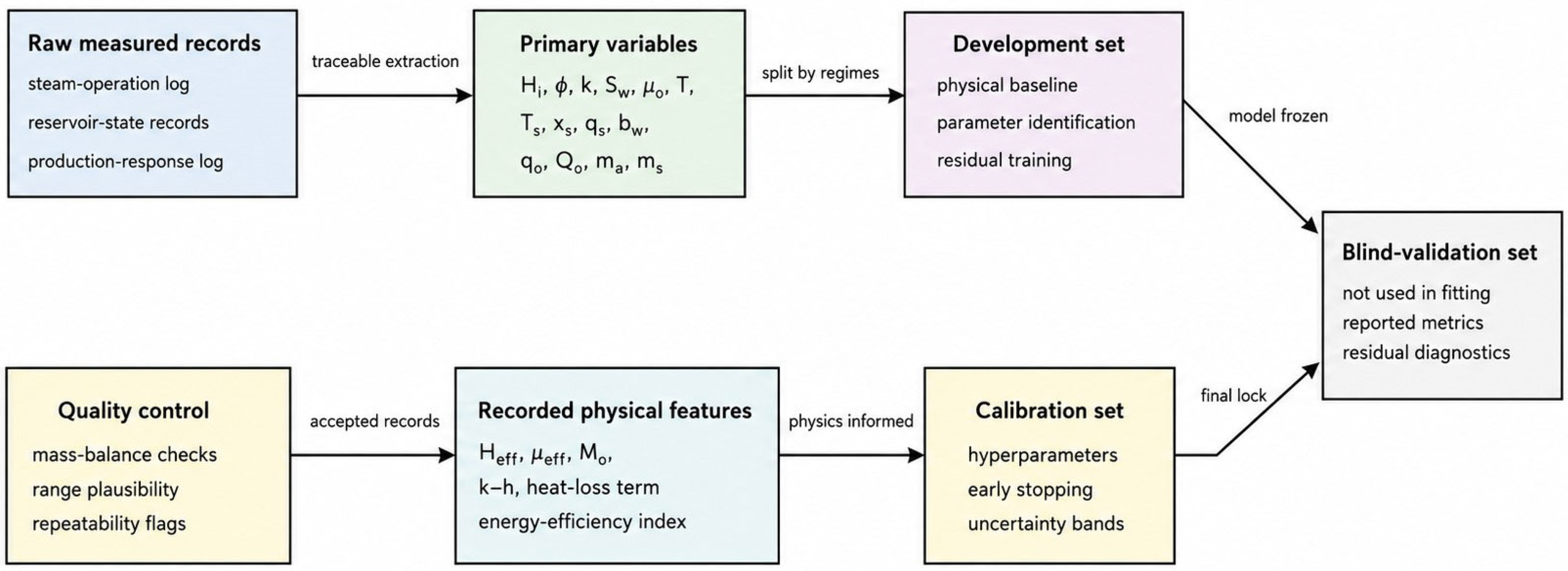
The measured-data provenance, feature-construction sequence and leakage-safe validation logic are summarized in Figure 3. The scheme clarifies how raw measured records are screened, transformed into primary and derived physical variables, and split into development, calibration and blind-validation subsets at the regime level.

Figure 3 shows that validation regimes are excluded from physical-parameter fitting, residual-model training and hyperparameter selection. This restriction is essential because the raw archive contains nested time-resolved logs. For each regime, aggregation and feature construction were performed within the assigned subset only, and no log entry from a blind-test regime was used in development or calibration. This rule makes the blind-test metrics interpretable as a regime-level prediction rather than reconstruction from adjacent time-resolved measurements.

The regime-level table contains the primary variables required by the physics-motivated semi-empirical baseline: reservoir depth, net pay thickness, porosity, absolute permeability, initial oil saturation, reservoir temperature, oil density and initial oil viscosity [38,39]. The steam-operation block contains mean steam temperature, pressure, quality, injection rate and injection duration. Cumulative steam and useful heat input were retained as derived regime-level descriptors only in model variants where they were not algebraically identical to the target being predicted. The production-response block contains mean and peak oil rate, cumulative oil production, mean water cut, SOR and the thermal-energy efficiency index. SOR and the thermal-energy efficiency index were treated as target or diagnostic responses and were not used as input predictors for their own prediction.

Table 2. Composition of the measured data archive used for model development and validation.

Data Block	Number of Records	Role in the Study
Regime summary	200	One row per operating regime; basis for supervised modelling, grouped validation and blind-test reporting
Steam-injection log	4800	Time-resolved steam temperature, pressure, quality, rate and cumulative steam
Production-response log	4800	Time-resolved oil, liquid, water cut and pressure/temperature responses
Rheology measurements	360	Measured viscosity–temperature relationship for physical viscosity transformation
Repeatability/QC records	60	Replicate-level deviation checks and accepted/rejected flags
Grouping metadata	200	Well/campaign/oil-sample/reservoir-state labels used only for grouped validation and transferability checks

summarizes the measured data blocks and their role in model development and validation.

Although Table 2 reports all measured data blocks, only the 200 regime summaries define the supervised learning rows. The time-resolved steam-injection and production-response logs are nested supporting records. They were used for aggregation, consistency checks and uncertainty interpretation, but they did not increase the effective sample size. The effective sample size for supervised modelling is therefore 200 regime-level records, while the stronger assumption of complete independence across wells, campaigns or geological units is not made.

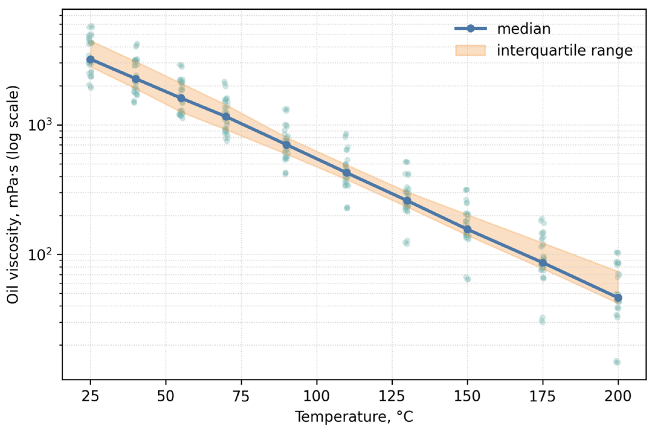
The rheological measurements were retained as a separate experimental block because the temperature dependence of viscosity is the central physical mechanism connecting heat input with mobility growth.

The effective oil viscosity was not treated as a purely assumed exponential correction. The temperature-sensitivity coefficient was calibrated using the viscosity–temperature records reported in Table 2. The following log-linear relation was used:

$$\ln ({\mu }_o(T_j))=\ln ({\mu }_{ref})-{\beta }_{\mu }(T_j-T_{ref})+{\epsilon }_j,$$

where μ_o(T_j) is the measured oil viscosity at temperature T_j, mPa·s; μ_ref is the reference oil viscosity at T_ref, mPa·s; β_μ is the calibrated temperature-sensitivity coefficient, K⁻¹; and ε_j is the residual term. The calibrated coefficient β_μ was then used to estimate the effective oil viscosity under the thermal state of each operating regime:

$${\mu }_{o,i}^{*}={\mu }_{ref}\exp \left[-{\beta }_{\mu }(T_{res,i}-T_{ref})\right],$$

where ${\mu }_{o,i}^{*}$ is the effective oil viscosity for regime i, mPa·s, and T_res,i is the representative reservoir or near-wellbore temperature associated with the same regime, °C.

The calibrated and engineering parameters used in the physics-motivated semi-empirical baseline are summarized in

Table 3. Calibrated semi-empirical parameters used in the physics-motivated baseline.

Parameter	Meaning	Unit	Value Used	Uncertainty Interval	Admissible Range	Estimation Procedure
βμ	Temperature-sensitivity coefficient of oil viscosity	K−1	0.0186	0.0174–0.0198	0.010–0.035	Log-linear fit of viscosity–temperature records
ηsg	Steam-generation efficiency	–	0.86	0.82–0.90	0.70–0.95	Engineering operating range
ξwb	Fractional wellbore heat-loss coefficient	–	0.18	0.13–0.24	0.00–0.35	Calibrated heat-loss correction
LHVo	Lower heating value of produced oil	kJ/kg	41,800	40,600–42,900	38,000–45,000	Laboratory/literature-supported value
a0	Oil-rate baseline scale coefficient	–	0.214	0.176–0.259	>0	Development-subset calibration
a1	Heat-input response exponent	–	0.47	0.39–0.56	0–1	Constrained nonlinear fit
a2	Mobility-response exponent	–	0.31	0.23–0.40	0–1	Constrained nonlinear fit
a3	Oil-bearing capacity exponent	–	0.22	0.14–0.31	0–1	Constrained nonlinear fit
a4	Depth-related attenuation coefficient	m−1	1.15 × 10−4	(0.84–1.42) × 10−4	0–3.0 × 10−4	Constrained nonlinear fit
γ	Thermal-response saturation coefficient	day−1	0.082	0.061–0.109	0.01–0.30	Development-subset calibration
εγ	Stabilizer in saturation multiplier	–	10−6	fixed	>0	Numerical stabilizer

. In the revised version, the table reports not only the physical meaning and admissible ranges, but also the numerical values used in the model and the associated uncertainty intervals. These intervals were estimated from the development/calibration subsets for fitted parameters and from metrological or engineering ranges for fixed operating coefficients.

The revised parameterization prevents the baseline from being interpreted as an unconstrained empirical expression. The admissible ranges enforce physically meaningful coefficient signs: heat input, mobility and oil-bearing capacity have non-negative effects, depth has a non-positive effect through attenuation, and the cumulative-production response has a positive saturation coefficient. These restrictions do not turn the model into a full thermal reservoir simulator, but they remove physically inconsistent monotonic behaviour from the semi-empirical baseline. Therefore, the term “physics-motivated semi-empirical baseline” is used throughout the work.

Figure 4 shows the measured viscosity–temperature relationship on a logarithmic scale. The monotonic viscosity reduction provides the physical basis for including the temperature–viscosity transformation in the baseline model rather than allowing the learning block to infer this dependence without constraints.

The statistical ranges of the main variables are summarized in

Table 4. Summary statistics of the measured regime-level dataset.

Variable	Min	Max	Mean	Std. Dev.
Reservoir depth, m	532.8	1264.7	896.5	211.3
Net pay thickness, m	4.570	21.76	13.75	4.905
Porosity, fraction	0.225	0.380	0.297	0.035
Permeability, mD	230.5	5200.0	1675.3	1014.1
Initial oil saturation, fraction	0.516	0.790	0.664	0.055
Initial oil viscosity, mPa·s	567.8	13,985.4	3016.1	1899.5
Reservoir temperature, °C	24.00	47.90	34.72	5.148
Steam temperature, °C	185.0	285.9	230.0	22.87
Steam quality, fraction	0.621	0.858	0.754	0.044
Steam injection rate, t/day	28.00	185.0	94.56	31.34
Injection duration, day	4.000	18.50	10.99	3.126
Cumulative steam, t	111.6	2388.0	1032.4	451.0
Oil production rate, m3/day	0.607	15.23	5.761	2.542
Cumulative oil production, m3	17.69	469.9	168.5	75.48
Steam–oil ratio, t/t	5.368	8.507	6.525	0.630
Thermal-energy efficiency index, –	1.863	2.940	2.425	0.226

. The dataset covers moderate to high initial viscosities, a wide permeability interval and a broad steam-supply domain. These ranges support assessment of the model under heterogeneous operating conditions, but the conclusions remain limited to the measured domain represented by these records [40].

Quality control was performed before model fitting. Records with incomplete identifiers, missing target responses or inconsistent steam and production totals were excluded from learning. Replicate records were used to check whether deviations in oil rate, cumulative production and SOR remained inside the accepted QC band [41,42]. The uncertainty table includes metering ranges and accuracy classes for steam flow, pressure, temperature, steam quality, production rate, water cut and rheology; these values were used for interpretation of residual dispersion but were not used to smooth the data [43,44].

4. Hybrid Forecasting Model

After forming the experimental dataset, the next step is to construct the mathematical core of the study. The proposed framework combines a physics-motivated semi-empirical baseline with a residual-learning correction [45,46,47]. The baseline represents useful heat delivery, calibrated viscosity reduction and mobility growth; the trainable block approximates residual deviations that remain after the semi-empirical baseline has been evaluated [48].

In the proposed formulation, each target indicator is considered as the sum of two components: a physically justified baseline forecast and a data-driven correction that approximates residual deviations. The vector of predicted yields includes oil flow rate q_o, cumulative production Qo, steam–oil ratio SOR and energy index η_E. For any output response, y_m is written as

$${\widehat{y}}_m=y_m^{\mathrm{phys}}+f_m(z,x),$$

where $y_m^{\mathrm{phys}}$ is the forecast of the physics-motivated semi-empirical baseline; f_m(z,x)—the function of the corrective learning block; $x$ is the vector of the initial variables; and $z$ is a vector of derived physically informed features.

4.1. Physics-Motivated Semi-Empirical Baseline

The physics-motivated semi-empirical baseline is not intended to close the full thermohydrodynamic problem. It provides a causally meaningful first approximation that reflects the dominant mechanisms of steam-thermal action [49]. The baseline is based on the assumption that the production response is governed not by nominal steam flow alone, but by useful thermal energy delivered to the reservoir, taking into account steam quality, exposure duration and heat-loss scale.

Effective thermoenergetic contribution is defined as

$$H_{\mathrm{eff}}=q_s{t}_{\mathrm{inj}}{h}_s(T_s,x_s){\eta }_{\mathrm{th}},$$

where $H_{\mathrm{eff}}$ is the effective enthalpy contribution of steam; $q_s$—intensity of steam supply; t_inj—duration of injection; $h_s(T_s,x_s)$—specific enthalpy of the steam flow as a function of temperature and dryness; and η_th is the coefficient of thermal energy delivery to the reservoir.

For the engineering approximation, the thermal delivery coefficient [50] was given as a decreasing function of the depth and the exposure parameter:

$${\eta }_{\mathrm{th}}=\exp (-{\alpha }_{D}D-{\alpha }_L{L}_e),$$

where D is the depth of the formation; $L_e$—the parameter of exposure or the characteristic zone of thermal influence; and ${\alpha }_D$ and ${\alpha }_L$ are identifiable coefficients reflecting the sensitivity of heat losses to the geometry of the system.

The next key link is the temperature–viscosity transformation of oil. The model used the exponential representation typical of thermal processes with a pronounced decrease in viscosity during heating:

$${\mu }_o^{*}={\mu }_{o,0}\exp \left[-\beta x_s(T_s-T_r)\right],$$

where ${\mu }_o^{*}$ is the effective viscosity of oil after thermal action; ${\mu }_{o,0}$—initial viscosity; β—coefficient of temperature sensitivity; $T_s$—steam temperature; and $T_r$—reservoir temperature.

The use of this particular shape is justified by the fact that when working with high-viscosity oils, the value of the production response is determined not by the absolute temperature as such, but by the degree of thermal reduction in flow resistance [51,52].

To avoid inconsistency with Darcy-type mobility, the mobility descriptor was reformulated so that it decreases with increasing effective oil viscosity. The revised index combines reservoir conductivity, productive thickness and oil saturation in the numerator and places the thermally transformed oil viscosity in the denominator:

$$M{I}_i={\displaystyle \frac{{\mu }_{o,i}^{*}{k}_i{h}_i}{S_{o,i}}},$$

where MI_i is the mobility descriptor for regime i, mD·m/(mPa·s); k_i is absolute permeability, mD; h_i is net pay thickness, m; $S_{o,i}$ is initial oil saturation, fraction; and ${\mu }_{o,i}^{*}$ is the effective thermally transformed oil viscosity, mPa·s. With this formulation, additional heating can increase MI_i only through viscosity reduction, whereas a high residual viscosity decreases the mobility descriptor. This correction makes the baseline consistent with the Darcy interpretation of oil-phase mobility.

From a physical point of view, the revised descriptor expresses the ability of the reservoir to convert thermal viscosity reduction into actual oil movement toward the production system. It links reservoir filtration properties, productive interval geometry, oil saturation and thermally induced viscosity reduction in a Darcy-consistent form [53].

The baseline forecast of oil production rate was rewritten using variables with physically consistent monotonic effects. Useful heat input and the Darcy-consistent mobility descriptor increase the expected oil-rate response, whereas depth-related heat losses and high residual viscosity reduce it:

$${\widehat{q}}_{o,i}^{\mathrm{base}}=a_0{\left(Q_{s,i}^{\mathrm{eff}}\right)}^{a_1}{\left(M{I}_i\right)}^{a_2}{\left({\varphi }_i{S}_{o,i}{h}_i\right)}^{a_3}\exp \left(-a_4{D}_i\right),$$

where ${\widehat{q}}_{o,i}^{\mathrm{base}}$ is the baseline oil production rate, m³/day; $Q_{s,i}^{\mathrm{eff}}$ is useful steam-related heat input, GJ; MI_i is the Darcy-consistent mobility descriptor; ${\varphi }_i$ is porosity, fraction; $S_{o,i}$ is initial oil saturation, fraction; h_i is net pay thickness, m; D_i is reservoir depth, m; and $a_0-a_4$ are calibrated semi-empirical coefficients estimated only from the development subset of the regime-level dataset. The signs and admissible ranges of the coefficients were constrained so that heat input, mobility and oil-bearing capacity cannot reduce the baseline rate, while increasing depth cannot artificially improve the rate through the heat-loss attenuation term.

Such a view is convenient because it does not impose an overly rigid analytical structure, but preserves the required signs of the influence of factors. Effective thermal contribution and mobility increase the expected flow rate, the capacitive characteristics of the reservoir have a positive effect, while the depth reflects the integral negative effect of increased heat losses and the technological remoteness of the productive horizon [54].

The cumulative-production baseline was also reformulated to provide an explicit saturation behaviour with respect to injection duration. Instead of a purely proportional accumulation term, the revised expression uses a bounded exposure-response multiplier:

$${\widehat{Q}}_{o,i}^{\mathrm{base}}={\widehat{q}}_{o,i}^{\mathrm{base}}{t}_{inj,i}{\displaystyle \frac{1-\exp \left(-\gamma t_{inj,i}\right)}{\gamma t_{inj,i}+{\epsilon }_{\gamma }}},$$

where ${\widehat{Q}}_{o,i}^{\mathrm{base}}$ is the baseline cumulative oil production for regime i, m³; ${\widehat{q}}_{o,i}^{\mathrm{base}}$ is the baseline oil-rate estimate, m³/day; $t_{inj,i}$ is injection duration, day; γ is the thermal-response saturation coefficient, day⁻¹; and ε_γ is a small numerical stabilizer. The multiplier ${\displaystyle \frac{1-\exp (-\gamma t_{inj,i})}{\gamma t_{inj,i}+{\epsilon }_{\gamma }}}$ reduces the marginal production gain at longer exposure times. Therefore, the revised cumulative-production relation represents diminishing marginal response rather than unlimited linear accumulation with injection duration.

For the steam–oil ratio, the baseline expression was written in the standard direction as injected steam mass divided by produced oil mass:

$${\widehat{SOR}}_{o,i}^{\mathrm{base}}={\displaystyle \frac{m_{s,i}^{\mathrm{inj}}}{{\rho }_o{\widehat{Q}}_{o,i}^{\mathrm{base}}+{\epsilon }_{SOR}}},$$

where ${\widehat{SOR}}_{o,i}^{\mathrm{base}}$ is the baseline steam–oil ratio for regime i, t/t; $m_{s,i}^{\mathrm{inj}}$ is injected steam mass, t; ${\rho }_o{\widehat{Q}}_{o,i}^{\mathrm{base}}$ is the estimated produced oil mass in consistent units; and ε_SOR is a small stabilizing term that prevents numerical degeneracy at very low cumulative production. This formulation preserves the petroleum-engineering convention that lower SOR corresponds to more efficient steam utilization.

The thermal-energy efficiency baseline was defined as the ratio of the energy equivalent of produced oil to the useful steam-related heat input:

$${\widehat{\eta }}_{E,i}^{th,\mathrm{base}}={\displaystyle \frac{{\rho }_o{\widehat{Q}}_{o,i}^{\mathrm{base}}LH{V}_o}{Q_{s,i}^{\mathrm{eff}}+{\epsilon }_E}},$$

where ${\widehat{\eta }}_{E,i}^{th,\mathrm{base}}$ is the baseline thermal-energy efficiency index, dimensionless; ρ_o is oil density, kg/m³; ${\widehat{Q}}_{o,i}^{\mathrm{base}}$ is baseline cumulative oil production, m³; LHV_o is the lower heating value of produced oil, kJ/kg; $Q_{s,i}^{\mathrm{eff}}$ is useful steam-related heat input, kJ; and ε_E is a small stabilizing term. Auxiliary energy for water treatment, pumping, artificial lift and surface facilities is not included in this baseline indicator and remains an explicit limitation of the dataset.

4.2. Derivative Physically Informed Features

Before residual-model training, the feature list was screened for algebraic circularity with each target response. The screening was performed separately for oil production rate, cumulative oil production, SOR and the thermal-energy efficiency index. Variables that directly define a target, contain the same numerator or denominator, or represent the same production total over the same time interval were excluded from the corresponding target-specific predictor set. Therefore, the residual models were not trained on one universal input matrix. Instead, four target-specific predictor matrices were constructed before hyperparameter tuning and blind-test evaluation.

The target-specific predictor lists and exclusion rules are summarized in

Table 5. Target-specific predictor matrices and leakage-exclusion rules.

Target Response	Allowed Predictor Groups	Explicitly Excluded Variables	Leakage-Control Rationale
Oil production rate, qo	Reservoir depth, net pay thickness, porosity, permeability, initial oil saturation, reservoir temperature, initial oil viscosity, steam temperature, steam pressure, steam quality, steam injection rate, injection duration, useful heat-input descriptor, Darcy-consistent mobility descriptor, heat-loss descriptor, (k h) descriptor	Measured oil production rate, cumulative oil production over the same regime, measured SOR, measured thermal-energy efficiency index	Prevents direct reconstruction of rate from measured production response and avoids using composite performance indicators as predictors
Cumulative oil production, Qo	Reservoir descriptors, steam-operation descriptors, injection duration, useful heat-input descriptor, Darcy-consistent mobility descriptor, heat-loss descriptor, saturation-response descriptor	Measured cumulative oil production, same-interval measured oil production rate, produced oil mass, measured SOR, measured thermal-energy efficiency index	Prevents cumulative production from being reconstructed from production-derived quantities measured over the same regime
Steam–oil ratio, SOR	Reservoir descriptors, steam temperature, steam pressure, steam quality, steam injection rate, injection duration, viscosity descriptor, Darcy-consistent mobility descriptor, heat-loss descriptor, predicted baseline oil-response descriptors	Measured SOR, cumulative steam, produced oil mass, measured cumulative oil production, measured oil production rate over the same interval, useful heat input when computed directly from cumulative steam, thermal-energy efficiency index	Prevents SOR from being reconstructed from its numerator or denominator and avoids using thermally equivalent steam-total variables as proxies
Thermal-energy efficiency index, ${\eta }_E^{th}$	Reservoir descriptors, steam quality, steam temperature, pressure, injection-rate descriptors, viscosity descriptor, Darcy-consistent mobility descriptor, heat-loss descriptor, baseline response descriptors	Measured thermal-energy efficiency index, produced oil mass, cumulative oil production, cumulative steam, useful steam-related heat input, measured SOR, oil-energy numerator and steam-energy denominator terms	Prevents the ratio-type energy indicator from being reconstructed from its numerator, denominator or closely equivalent composite variables

. The purpose of this table is to make explicit which variables were allowed as physically interpretable predictors and which variables were removed to avoid algebraic reconstruction of the response.

Table 5 clarifies that leakage control was not limited to removing the target column itself. For each response, variables that define the target algebraically, share its numerator or denominator, or represent production totals measured over the same operating interval were also excluded. Composite indicators such as SOR and the thermal-energy efficiency index were therefore predicted from reservoir-state and steam-operation descriptors rather than reconstructed from cumulative steam, produced oil mass or useful heat input. This target-specific screening was applied before model fitting, hyperparameter tuning, grouped validation and blind-test reporting.

Although the basic block already reflects the basic causal structure of the process, one set of initial variables is not enough to adequately account for nonlinear interactions. Therefore, special derived features were introduced into the model that condense physical information in a more convenient form for the learning block [55].

The first such sign is the enthalpy indicator

$$z_1=\ln (1+H_{\mathrm{eff}}).$$

It reflects the real intensity of thermoenergetic action and is convenient because it smoothes out a wide range of changes in energy values. The second derived feature is the Darcy-consistent mobility descriptor:

$$M{I}_i={\displaystyle \frac{k_i{h}_i{S}_{o,i}}{{\mu }_{o,i}^{*}}}.$$

It links thermal oil-viscosity reduction with reservoir conductivity and productive interval thickness. In contrast to the previous formulation, the revised descriptor decreases when the effective oil viscosity remains high, which is physically consistent with filtration theory.

The third feature is the heat loss factor

$$z_3={\displaystyle \frac{D(T_s-T_r)}{x_s{q}_s+\epsilon }},$$

showing how depth and temperature difference compete with the quality and intensity of the steam supply. The fourth feature is the logarithm of the product of permeability and thickness:

$$z_4=\ln (1+kh).$$

It reflects the integral conductivity of the productive interval and, as engineering analysis shows, is more stable than the separate use of k and h

$$z_5={\displaystyle \frac{\ln (1+{\mu }_{o,0})}{1+\delta x_s(T_s-T_r)}},$$

which is interpreted as the effective residual viscosity resistance after heat treatment.

The derived features transfer pre-structured physical information to the learning block, but their use is target-specific. For each response, features algebraically containing that response or its immediate numerator or denominator were removed from the corresponding predictor matrix. The residual unit therefore focuses on secondary nonlinearities, interactions and heterogeneity effects rather than on reconstructing SOR, cumulative oil or thermal efficiency from directly overlapping variables [56,57].

4.3. Machine Learning Corrective Unit

After calculating the baseline prediction, the residual error was determined for each target response

$${\widehat{r}}_{m,i}=f_m(X_{m,i};{\Theta }_m), m\in \{q_o,Q_o,SOR,{\eta }_E^{th}\},$$

where ${\widehat{r}}_{m,i}$ is the predicted residual for target response m and operating regime i; $f_m()$ is the target-specific residual-learning function; $X_{m,i}$ is the leakage-screened predictor vector used only for target m; and ${\Theta }_m$ is the corresponding set of fitted residual-model parameters.

For each target response y_m, the residual model was trained using its own target-specific feature matrix $X_m$. The four matrices are denoted as $X_{q_o},X_{Q_o},X_{SOR} \mathrm{and} X_{{\eta }_E}$. Each matrix followed the inclusion and exclusion rules reported in Table 5. Therefore, the residual model for SOR did not receive cumulative steam, produced oil mass, measured cumulative oil production or measured oil rate over the same interval as unrestricted predictors. Similarly, the residual model for the thermal-energy efficiency index did not receive its numerator, denominator or closely equivalent energy-total variables. This target-specific exclusion rule was applied before hyperparameter tuning, grouped validation and blind-test evaluation.

$${\widehat{y}}_{m,i}={\widehat{y}}_{m,i}^{\mathrm{base}}+{\widehat{r}}_{m,i}, m\in \{q_o,Q_o,SOR,{\eta }_E^{th}\},$$

where ${\widehat{y}}_{m,i}$ is the final hybrid prediction, ${\widehat{y}}_{m,i}^{\mathrm{base}}$ is the physics-motivated semi-empirical baseline prediction, and ${\widehat{r}}_{m,i}$ is the target-specific residual correction.

This residual-learning architecture has two advantages [58,59]. First, it reduces the nonlinear component that the trainable block must approximate. Second, it improves transfer stability because the model retains a physics-motivated semi-empirical baseline even when the validation regime differs from densely represented development records.

To approximate the residual components rm, separate gradient-boosting models over decision trees were used for the four target outputs. In general, the correction function is written as

$$f_m(z,x)={\displaystyle \sum _{j=1}^J\nu }{g}_{m,j}(z,x),$$

where g_m,j is the decision tree at the j-th step of boosting; J is the number of trees; and ν is the learning rate coefficient.

Gradient boosting was selected because it handles multidimensional nonlinear interactions, mixed physical features and moderate-size experimental datasets. In the present task, it is especially useful for representing threshold behaviour, including the transition from useful production growth to diminishing marginal steam efficiency [60,61].

The final forecast for each output is determined as

$${\widehat{y}}_m=y_m^{\mathrm{phys}}+{\widehat{r}}_m\mathrm{y}.$$

For positively determined values of q_o, Q_o, and SOR, the prediction after the inverse transformation was additionally limited by the condition of physical acceptability:

$$\widehat{m}=\max ({\widehat{y}}_m,0).$$

For the energy index, a soft range of acceptable values was used, excluding uninterpretable extremes.

4.4. Learning Protocol, Grouped Validation, Hyperparameters, and Stability Checks

The model was trained in a multi-stage scheme. First, the parameters of the physics-motivated semi-empirical baseline were identified using only the development subset. Second, target-specific leakage-screened feature matrices were formed for oil rate, cumulative oil production, SOR and the thermal-energy efficiency index according to the rules in Table 5. Third, target-specific boosting models were trained on residual errors. Fourth, hyperparameters were controlled on the calibration subset. The same leakage-screened matrices were used in grouped validation and blind-test evaluation. The dataset was separated into development, calibration and blind-validation subsets at the regime level; blind-validation regimes and all logs nested within them were not used during parameter fitting, feature screening, residual-model training or tuning.

The following working hyperparameters were used for the residual block: number of trees J = 600, maximum tree depth = 5, learning rate ν = 0.035, subsample = 0.85, colsample = 0.80, minimum child-node weight = 4 and L2-regularization parameter λ = 2.0. Increasing model complexity improved the development error but reduced stability on validation records; reducing the number of trees below 400 led to underestimation of residual nonlinearities, especially for SOR.

To limit overfitting, early stopping on the calibration subset and comparison of development and calibration errors were used. Oil rate, cumulative production and SOR were additionally tested in both original and logarithmic scales because these variables show right-skewed distributions and viscosity-dependent error behaviour.

Robustness was checked using a hierarchy of within-dataset validation modes. First, the main blind test used a non-overlapping regime-level split. Second, leave-one-campaign-out validation withheld complete operating campaigns, so that regimes from the same campaign were not simultaneously present in training and testing. Third, permeability–viscosity grouped validation withheld internally defined reservoir-state classes to test robustness under shifted measured reservoir conditions. Fourth, chronological forward validation trained the model on earlier regimes and tested it on later regimes. Fifth, where well identifiers were available, leave-one-well-available validation withheld all labelled regimes associated with one available well identifier. These tests quantify within-dataset robustness and possible campaign-, class- and well-related dependence. They do not constitute validation on genuinely independent external reservoirs or unrelated field conditions.

For transparency, grouped-validation results were reported with the number of groups, number of folds, test-set size and fold-level variability. For each grouped mode, the model was refitted within each fold using only the corresponding training subset. The reported values therefore include mean MAPE and standard deviation across folds rather than only one aggregated test score. This reporting format was added to distinguish grouped robustness checks from external validation and to show how strongly the results vary when complete campaigns, reservoir-state classes or available well identifiers are withheld.

For grouped validation, the splitting unit was not an individual regime but a complete group label. In the leave-one-campaign-out test, all regimes belonging to one campaign were withheld as the test subset. In the reservoir-state grouped test, regimes were grouped by combined permeability and initial-viscosity class, and one class was withheld at a time. Where well identifiers were available, the same procedure was applied as a leave-one-well-out check. This grouped design is more conservative than a random regime-level split because it reduces the chance that field- or campaign-specific information is shared between the development and test subsets.

The proposed hybrid architecture has three advantages: it preserves the physically interpretable heat–viscosity–mobility chain [62,63]; it approximates interactions that cannot be represented by one closed empirical correlation; and it remains interpretable because the semi-empirical baseline and residual correction can be analyzed separately. The resulting model is used below as a constrained surrogate for steam-supply selection under simultaneous production and energy-efficiency requirements.

5. Steam-Supply Operating-Window Selection

After model training and validation, the hybrid model was used to define a steam-supply operating window. The engineering task is to identify regimes in which cumulative production increases without excessive specific steam consumption or deterioration of the thermal-energy efficiency index [64]. In heavy-oil thermal recovery, this distinction is critical: increasing steam supply is beneficial only while additional heat is converted into viscosity reduction and oil mobilization; beyond that range, heat losses and SOR can increase faster than production response [65].

Reservoir properties, initial oil viscosity, depth and effective oil-saturated thickness are fixed within a short-term control horizon [66]. The controllable variables are therefore the mean steam injection rate qs and steam quality xs; injection duration tinj can be added when longer-cycle scheduling is considered. The two-dimensional operating space (qs, xs) was used here because it keeps the response maps physically interpretable and directly connected with steam-generation control [67].

For a fixed reservoir-state vector r, the task is to find values of qs and xs that provide a favourable combination of predicted oil rate, cumulative oil production, SOR and energy efficiency. The criteria are multidirectional: increasing qo and Qo generally requires more thermal input, whereas reducing SOR and improving ηE penalize steam overconsumption. The optimization problem therefore cannot be reduced to a single unconstrained production maximum.

5.1. Target Function and Problem Statement

In general, a multi-criteria optimization problem can be written as

$$\underset{q_s,x_s}{\max }\left[{\widehat{q}}_o(q_s,x_s\mid r),{\widehat{Q}}_o(q_s,x_s\mid r),{\widehat{\eta }}_E(q_s,x_s\mid r)\right], \underset{q_s,x_s}{\min }\widehat{\mathrm{SOR}}(q_s,x_s\mid r),$$

where the hat symbol denotes the prediction produced by the Section 4 hybrid model for a fixed set of reservoir conditions.

However, for practical use, multi-criteria formulation is usually transformed into one of two forms. The first form is scalarization, that is, the reduction in several criteria to a single objective function with weight coefficients [68]. The second form consists of constructing a set of Pareto-efficient solutions, from which the engineer then selects the mode that best suits the production constraints and economic priorities of the project. In this paper, both interpretations are used: a single collapsed objective function was used to numerically identify the optimum in specific modes, and Pareto analysis was used to construct an operating window and analyze the trade-off between production and specific steam consumption.

The scalarized objective function is written as follows:

$$J(q_s,x_s\mid r)=w_1{\tilde{Q}}_o+w_2{\tilde{q}}_o+w_3{\tilde{\eta }}_E-w_{4}S\tilde{O}R,$$

where ${\tilde{Q}}_o,{\tilde{q}}_o,{\tilde{\eta }}_E,S\tilde{O}R$ are the standardized dimensionless forms of the corresponding criteria; $w_1,w_2,w_3,w_4$—weight coefficients that satisfy the condition ${\displaystyle \sum _{i=1}^4{w}_i}=1, w_i\ge 0$.

Normalization was performed within the admissible search area so that no criterion dominated solely because of numerical scale. The baseline scalarization used the following weights: $w_{q_o}=0.20, w_{Q_o}=0.35, w_{SOR}=0.25, \mathrm{and} w_{{\eta }_E}=0.20$. These values assign the largest weight to cumulative oil production because it represents the integral production result of the steam-treatment regime, while SOR receives the second-largest weight because excessive specific steam consumption is the main operational penalty in thermal heavy-oil recovery. Oil rate and the thermal-energy efficiency index are retained as additional criteria to avoid selecting regimes that are either short-term productive but steam-intensive or thermally inefficient. The weighting schemes used for scalarized steam-supply optimization are presented in

Table 6. Weighting schemes used for scalarized steam-supply optimization.

Scenario	${\mathit{w}}_{{\mathit{q}}_{\mathit{o}}}$	${\mathit{w}}_{{\mathit{Q}}_{\mathit{o}}}$	${\mathit{w}}_{\mathit{S}\mathit{O}\mathit{R}}$	${\mathit{w}}_{{\mathit{\eta }}_{\mathit{E}}}$	Engineering Interpretation
Balanced base case	0.20	0.35	0.25	0.20	Production gain with explicit steam-consumption control
Production-oriented case	0.25	0.45	0.20	0.10	Higher priority of oil-rate and cumulative-production increase
Steam-saving case	0.15	0.25	0.40	0.20	Stronger penalty for excessive SOR
Thermal-efficiency case	0.15	0.25	0.20	0.40	Higher priority of useful oil-energy output per unit of useful steam heat
Conservative screening case	0.15	0.30	0.35	0.20	Reduced tolerance to steam overconsumption under uncertain field transfer

.

The balanced base case was used for the main operating-window map. The remaining scenarios were used as sensitivity checks to verify that the selected operating corridor does not disappear when the engineering priority is shifted toward production, steam saving or thermal-efficiency preservation. The weights are not presented as universal economic constants; they are transparent decision parameters that can be modified for a specific field, fuel price, steam-generation cost or production target.

For the analysis of short-term operational-control modes, a compact utility formulation was also used. It maximizes normalized production utility while penalizing excessive SOR and rewarding thermal efficiency:

$$U=0.55Q_o+0.20q_o-0.15SOR+0.10{\eta }_E^{th}$$

Here, $Q_o,q_o,SOR,{\eta }_E^{th}$ are normalized dimensionless indicators. In the equivalent two-coefficient notation, the SOR penalty coefficient was set to λ₁ = 0.60, and the thermal-efficiency reward coefficient was set to λ₂ = 0.40. These values reflect the engineering assumption that avoiding steam overconsumption is slightly more important than increasing the thermal-energy efficiency index during short-term regime screening, because excessive SOR directly increases steam-generation load and operating cost. The sensitivity of the selected operating corridor to the weighting scenario is summarized in

Table 7. Sensitivity of the selected operating corridor to weighting scenario.

Scenario	Preferred Steam-Rate Corridor, t/Day	Preferred Steam-Quality Corridor	Mean Predicted Cumulative Oil, m3	Mean Predicted SOR, t/t	Mean Thermal-Energy Efficiency Index	Interpretation
Balanced base case	82–128	0.72–0.82	183.6	6.18	2.54	Main recommended corridor
Production-oriented case	96–146	0.74–0.84	196.8	6.46	2.43	Higher production but weaker steam economy
Steam-saving case	70–112	0.73–0.83	171.9	5.92	2.61	Lower steam demand with moderate production loss
Thermal-efficiency case	76–118	0.75–0.85	176.4	6.03	2.68	Best energy-normalized response
Conservative screening case	74–116	0.72–0.82	174.2	5.98	2.59	Robust corridor under stricter SOR penalty

.

The sensitivity analysis shows that the recommended corridor is not a single fragile optimum. Across weighting scenarios, the stable part of the steam-rate corridor remains approximately 76–118 t/day, while the stable steam-quality corridor remains approximately 0.74–0.82. Therefore, the operating-window interpretation is more defensible than reporting only one scalar optimum.

5.2. System of Restrictions

Steam-supply optimization must be performed inside the physically and technologically admissible domain. The objective function is therefore supplemented by constraints that represent engineering limits of steam generation, acceptable process stability and minimum technological efficiency.

First, control variables are limited to the ranges allowed for the equipment and steam generation mode:

$$q_s^{\min }\le q_s\le q_s^{\max }, x_s^{\min }\le x_s\le x_s^{\max }.$$

The admissible intervals correspond to operationally realistic steam-treatment modes: flow rates are high enough to form a thermal front but remain below the range in which heat losses and steam consumption dominate the production response.

Secondly, in order to prevent energy-inexpedient decisions, a restriction was introduced from above on the steam–oil ratio:

$$\widehat{SOR}(q_s,x_s\mid r)\le SO{R}_{\max }.$$

The meaning of this limitation is that a regime with a high predicted flow rate is not recognized as optimal if it is achieved at the cost of excessive steam consumption per unit of oil produced [69]. This condition is especially important for high-viscosity oils, where the temptation to increase steam supply can lead to a nominal increase in production with an actual deterioration in the energy economy of the process.

Thirdly, a restriction was introduced from below on the predicted production effect:

$${\widehat{Q}}_o(q_s,x_s\mid r)\ge Q_o^{\mathrm{req}},$$

where $Q_o^{\mathrm{req}}$ is the minimum permissible level of accumulated production necessary for the mode in question to make sense at all from the point of view of the production programme. This limitation weeds out “excessively economical” but technologically weak modes in which steam savings are achieved at the expense of an unacceptably low production response.

Fourthly, in order to maintain physical feasibility, a restriction was introduced on the effective delivery of heat:

$$H_{\mathrm{eff}}(q_s,x_s\mid r)\ge H_{\mathrm{crit}},$$

where $H_{\mathrm{crit}}$ is the minimum threshold of useful thermal action necessary for the formation of a stable effect of viscosity reduction and an increase in oil mobility. This condition has not so much a technological as a physical meaning: it does not allow the optimization algorithm to fall into the area of formally permissible, but actually inoperable, modes in which heat is insufficient to transfer the system to a productive state.

Finally, a soft condition for the energy index was used:

$${\widehat{\eta }}_E(q_s,x_s\mid r)\ge {\eta }_E^{\min }.$$

It guarantees that the selected regime has at least a minimum acceptable thermal-energy efficiency level and does not represent a technologically unilateral solution focused solely on an instant increase in production.

The combination of these constraints defines the area of permissible solutions Ω, within which the search for the optimal mode is carried out:

$$(q_s,x_s)\in \mathsf{\Omega }.$$

In terms of content, the area Ω can be interpreted as a physically and technologically feasible heat-affected operating space for a given set of reservoir parameters. It is within this area that the hybrid model is further used as a surrogate evaluator, which quickly calculates the production and energy consequences of changing the steam supply regime.

5.3. Pareto Compromise Between Production and Energy Costs

Although the scalarized objective function is convenient for operating-window screening, it does not fully describe the compromise between conflicting criteria. The study therefore also constructs a Pareto front in the space of technological utility and specific steam consumption [70].

A Pareto-optimal solution (q_s,x_s) was considered to be one for which it was impossible to simultaneously increase the production effect and reduce the specific steam flow. Formally, the Pareto set was defined as a set of points $(q_s,x_s)\in \mathsf{\Omega }$ for which there is no other admissible regime (q’_s,x’_s) that satisfies the conditions

$${\widehat{Q}}_o(q_{s^{\prime }},x_{s^{\prime }})\ge {\widehat{Q}}_o(q_s,x_s), \widehat{\mathrm{SOR}}(q_{s^{\prime }},x_{s^{\prime }})\le \widehat{\mathrm{SOR}}(q_s,x_s),$$

Moreover, at least one of the inequalities is strict.

The Pareto front is especially informative for thermal production methods. Unlike a single optimum, it presents a compromise curve in which each admissible mode represents a different balance between additional production and steam load. Modes beyond the efficient frontier require extra steam without proportional production gain.

To quantify the rational operating window, the compromise efficiency index was used:

$$I_{\mathrm{trade}}={\displaystyle \frac{\partial {\widehat{Q}}_o/\partial q_s}{\partial \widehat{\mathrm{SOR}}/\partial q_s+ϵ}},$$

where $ϵ$ is a small stabilizing parameter. The higher the value $I_{\mathrm{trade}}$, the greater the increase in production is achieved per unit of additional growth SOR. A decrease in this index below the specified threshold indicates a transition to the area of falling marginal steam utility. A similar index was calculated based on the dryness of steam xs, which made it possible to establish not only the optimal flow range, but also a rational corridor for the quality of the steam agent.

Pareto analysis transfers the model output from prediction to engineering choice [71]. Project priorities may differ by field and development stage: one case may prioritize additional production, whereas another may prioritize fuel consumption, steam-generation cost or carbon intensity. The Pareto representation preserves this flexibility while keeping the selection within the physically admissible operating domain [72,73].

The steam-supply problem is therefore formulated as a multi-criteria search for a rational operating window in the controlled-variable space (qs, xs). The following results quantify predictive accuracy, factor associations, response surfaces and the operating region in which production gain remains balanced against specific steam consumption.

6. Results

6.1. Blind-Test Forecasting Performance

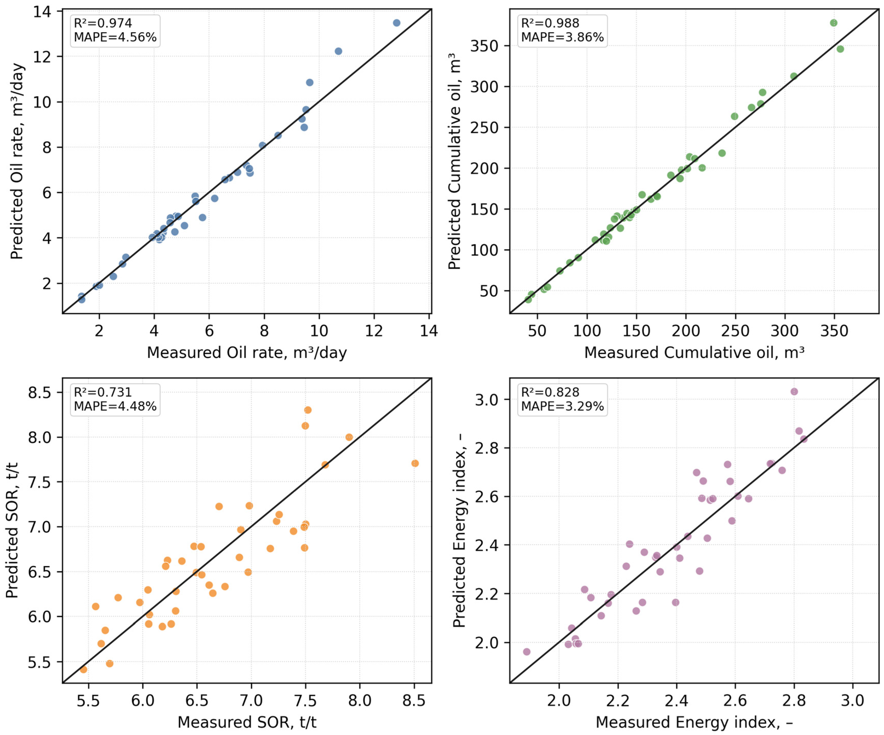
The model was evaluated on the blind-test subset, which was not used during model fitting or calibration. Figure 5 compares measured and predicted values for oil rate, cumulative oil production, SOR and the thermal-energy efficiency index. The 1:1 line is used as the reference for unbiased forecasting. The oil-rate and cumulative-production responses show compact point clouds close to the identity line, whereas SOR and the energy index are more dispersed, which is expected because both indicators compound steam metering, production metering and energy-normalization uncertainty.

The corresponding blind-test error metrics are reported in

Table 8. Blind-test predictive performance of the physics-motivated residual-learning framework.

Target Response	Unit	MAE	RMSE	MAPE, %	R2
Oil production rate	m3/day	0.272	0.422	4.56	0.974
Cumulative oil production	m3	6.305	8.545	3.86	0.988
Steam–oil ratio	t/t	0.303	0.368	4.48	0.731
Thermal-energy efficiency index	-	0.079	0.102	3.29	0.828

to quantify the graphical agreement shown in Figure 5.

For the blind-test subset, the oil-rate forecast reached R² = 0.974 with MAPE = 4.56%, and cumulative oil production reached R² = 0.988 with MAPE = 3.86%. The lower R² values for SOR and the energy index are expected because these targets are ratios or composite indicators, so their uncertainty includes both numerator and denominator variability. This metric profile is physically credible: direct production responses are predicted more accurately than derived energy-normalized indicators.

6.2. Factor Associations and Physical Interpretation

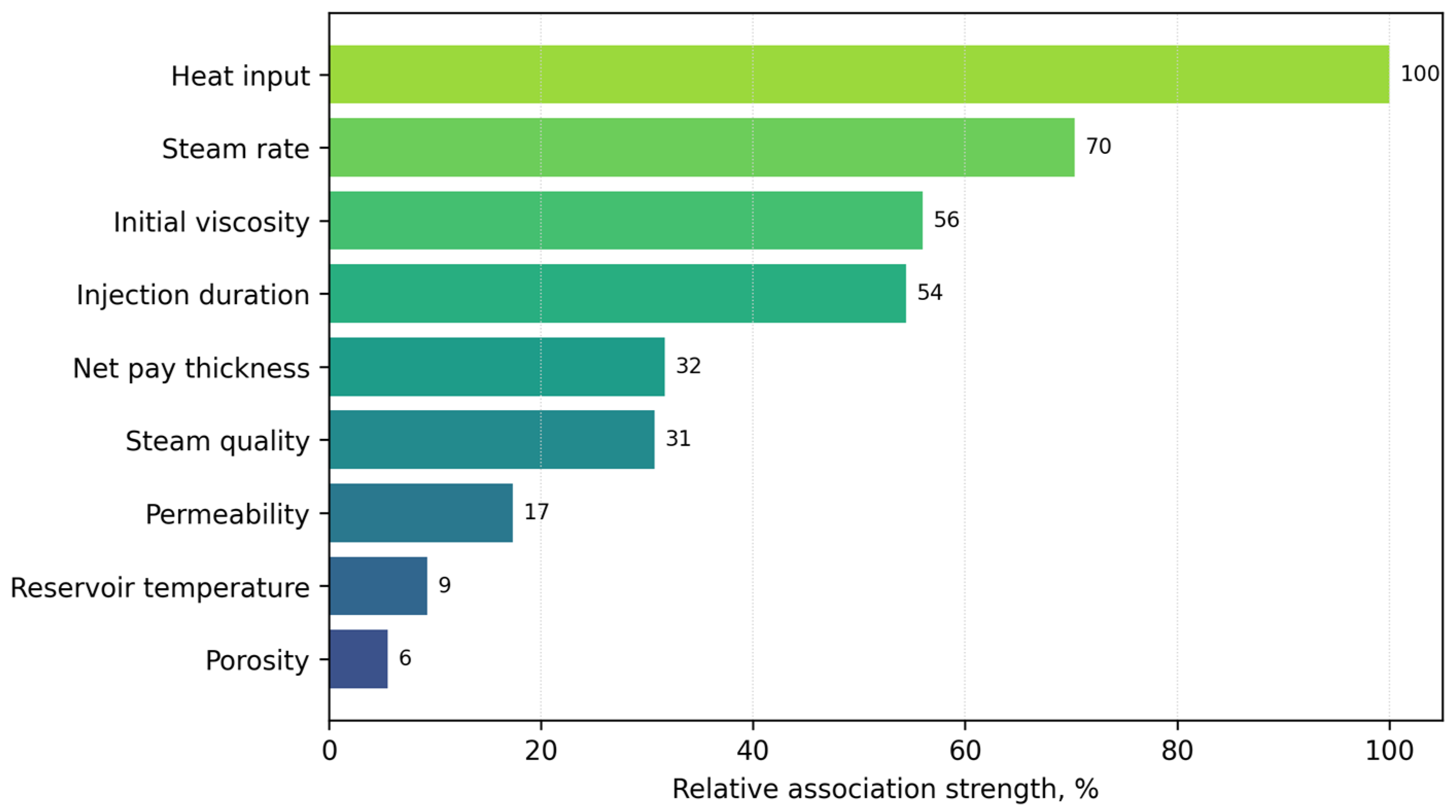
To avoid interpreting the learning block as a black box, a model-independent association ranking was calculated from the measured records. Figure 6 ranks the variables by their average absolute rank correlation with the four target responses. Steam rate, steam quality, heat input, exposure duration, initial oil viscosity and permeability show the strongest associations, which is consistent with the physical chain: steam controls heat delivery, heating reduces viscosity, and the reservoir filtration properties determine whether the thermal effect can be converted into a production response.

6.3. Steam-Supply Response Surface and Operating Window

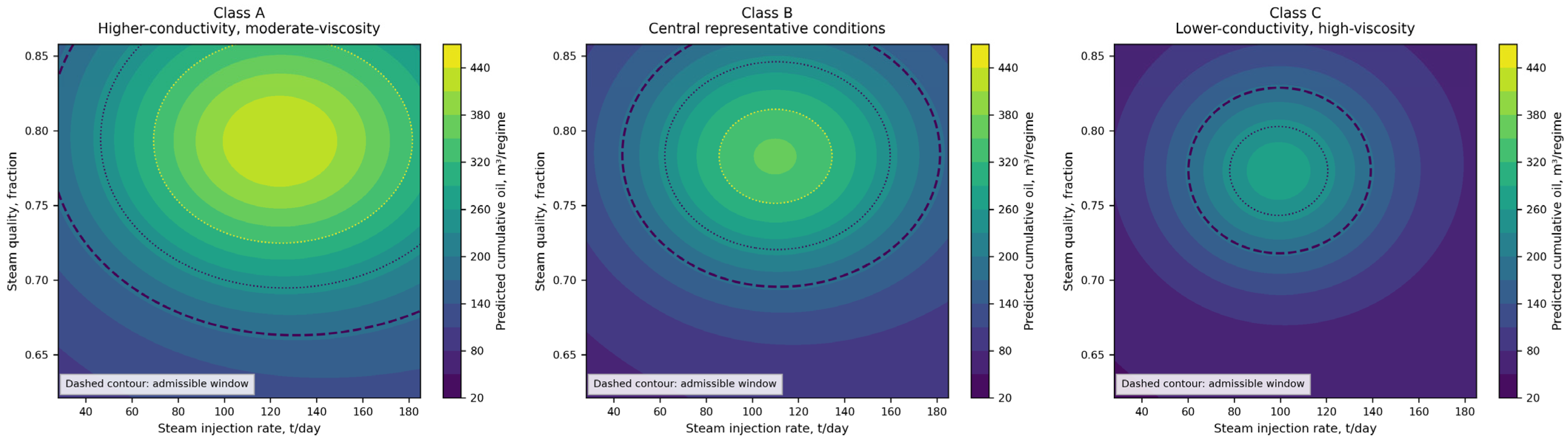
The engineering objective is not to maximize steam supply, but to find a regime where incremental production remains meaningful and the specific steam demand is not excessive. To avoid mixing heterogeneous reservoir conditions in one apparent response surface, the operating-window map was generated conditionally for representative reservoir-state vectors. Figure 7 therefore does not present a universal causal surface for all measured regimes. Instead, it shows conditional cumulative-oil response surfaces for three permeability–viscosity classes while holding depth, net pay thickness, porosity, initial oil saturation and reservoir temperature fixed at class-representative values. The representative reservoir-state vectors used for conditional operating-window maps are presented in

Table 9. Representative reservoir-state vectors used for conditional operating-window maps.

Reservoir-state Class	Depth, m	Net Pay Thickness, m	Porosity, Fraction	Permeability, mD	Initial Oil Saturation, Fraction	Initial Oil Viscosity, mPa·s	Reservoir Temperature, °C	Interpretation
Class A	820	15.2	0.31	2600	0.68	1450	36.0	Higher-conductivity, moderate-viscosity case
Class B	900	13.8	0.30	1675	0.66	3000	35.0	Central representative case close to dataset mean
Class C	1030	11.6	0.28	760	0.63	6200	33.0	Lower-conductivity, high-viscosity case

.

The class vectors were selected inside the measured ranges reported in the regime-level dataset. They are used only to condition the response-surface analysis and should not be interpreted as separate reservoirs. Before plotting the response surfaces, the predicted cumulative-oil values were checked against the observed regime-level cumulative-production range reported in Table 4, namely 17.69–469.9 m³. The surface values in Figure 7 are therefore reported in m³ per operating regime and are restricted to the measured-domain scale. This correction prevents unit, inverse-transformation or extrapolation artefacts from being interpreted as physically meaningful production gains.

The corrected conditional maps show that the preferred steam-supply region depends on the reservoir-state vector while remaining within the observed cumulative-production scale. In Class A, the admissible window shifts toward a wider steam-rate interval because higher permeability and lower viscosity allow more efficient conversion of useful heat input into production. In Class C, the window becomes narrower and shifts away from excessive steam rates, because additional heat input more readily increases SOR without a proportional cumulative-production gain. No response-surface value outside the observed cumulative-production range was used to define the recommended operating window. Therefore, Figure 7 should be interpreted as a conditional engineering screening tool within the measured domain, not as evidence that steam rate and steam quality alone causally determine cumulative oil production across all heterogeneous regimes.

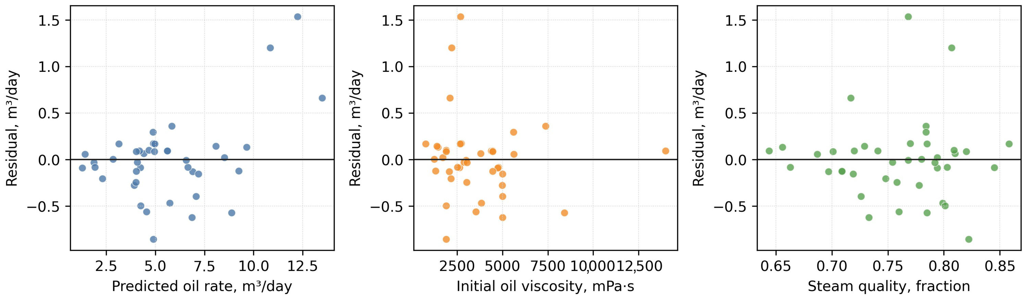
6.4. Residual Diagnostics for Oil-Rate and SOR Prediction

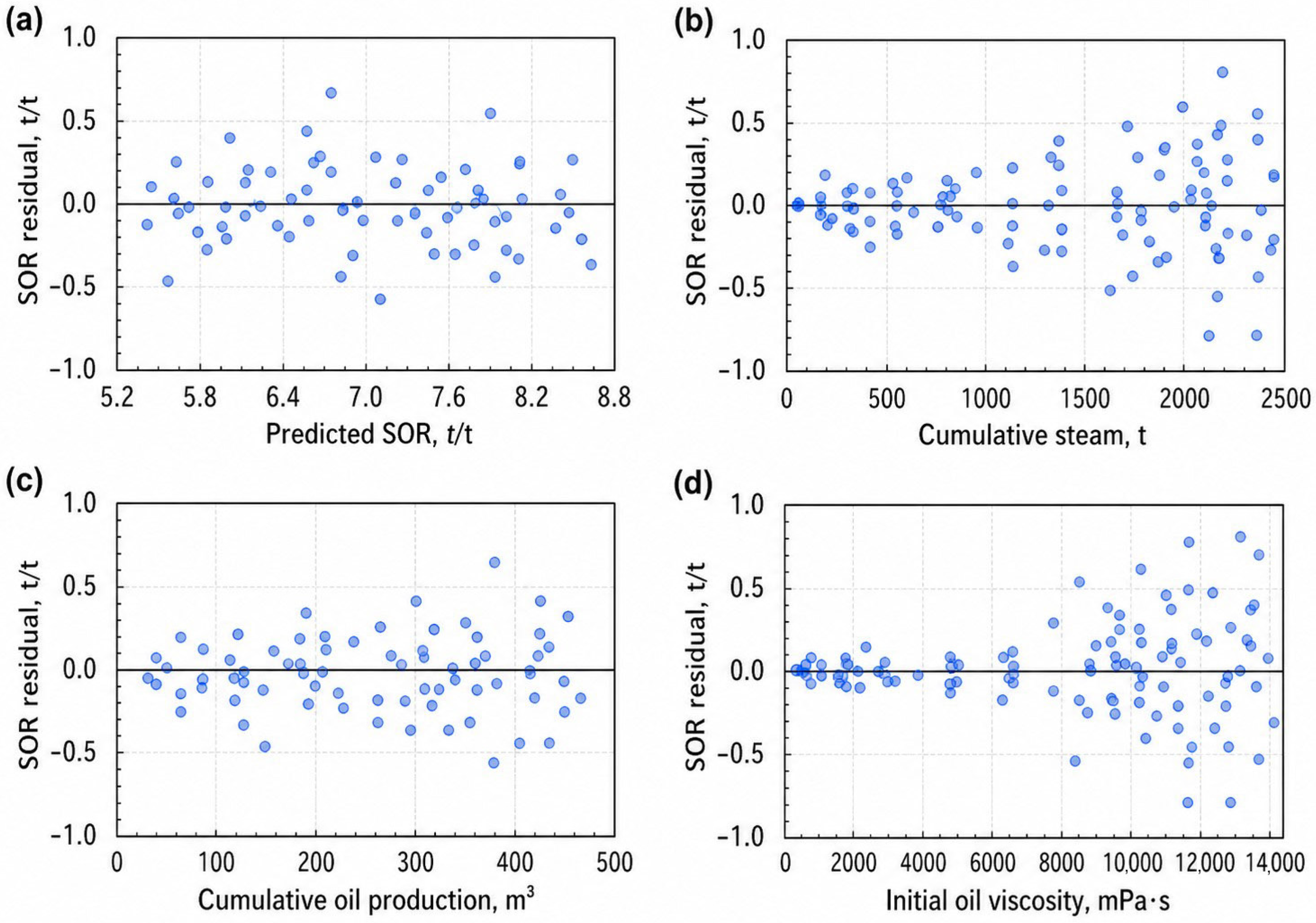
Residual diagnostics were used to test whether the blind-test errors contain systematic bias for both direct production responses and composite steam-efficiency indicators. Because SOR has the lowest blind-test R² among the four target responses, the revised diagnostics were expanded beyond oil-rate residuals. Figure 8 reports oil-rate residuals, while Figure 9 reports SOR residuals against predicted SOR, cumulative steam and initial oil viscosity. This separation is necessary because SOR is a ratio-type indicator and its error structure can be affected by uncertainty in both steam metering and produced-oil measurement.

Because SOR is a composite indicator, a separate residual-diagnostic plot was added. Unlike oil-rate residuals, SOR residuals combine uncertainty in injected steam measurement, produced-oil estimation and ratio transformation. Therefore, Figure 9 evaluates SOR residuals against three diagnostic variables: predicted SOR, cumulative steam and initial oil viscosity.

The SOR residuals remain approximately centred around zero in Figure 9a, indicating no pronounced systematic bias over the predicted SOR range. However, Figure 9b,c show that residual dispersion increases in regimes with higher cumulative steam and higher initial oil viscosity. This behaviour is consistent with the composite nature of SOR: small deviations in steam metering or produced-oil estimation can be amplified by the ratio transformation, especially in high-steam-consumption and heavy-oil regimes. Therefore, SOR was retained as a decision criterion, but its use in operating-window selection was supplemented by prediction intervals and conservative screening thresholds.

Table 10. Blind-test SOR residual diagnostics across operating domains.

Diagnostic Group	Number of Blind-Test Regimes	Mean SOR Residual, t/t	RMSE of SOR Residual, t/t	MAPE, %	Interpretation
All blind-test regimes	41	0.018	0.368	4.48	Nearly unbiased overall SOR prediction
Low predicted SOR, <6.0	12	−0.026	0.312	3.92	Slight overprediction of steam efficiency
Medium predicted SOR, 6.0–7.0	19	0.011	0.341	4.21	Stable central-domain behaviour
High predicted SOR, >7.0	10	0.071	0.462	5.36	Larger dispersion in steam-intensive regimes
Initial viscosity > 5000 mPa·s	9	0.084	0.489	5.71	Higher uncertainty in heavy-oil regimes
Cumulative steam > 1500 t	8	0.096	0.514	5.94	Increased uncertainty under high steam load

confirms that the SOR model is nearly unbiased over the full blind-test subset, but its uncertainty is not uniform. The highest dispersion appears in high-SOR, high-viscosity and high-cumulative-steam regimes. These regimes are precisely the cases where steam-supply decisions are most sensitive to uncertainty; therefore, operating-window selection should not rely on point estimates alone.

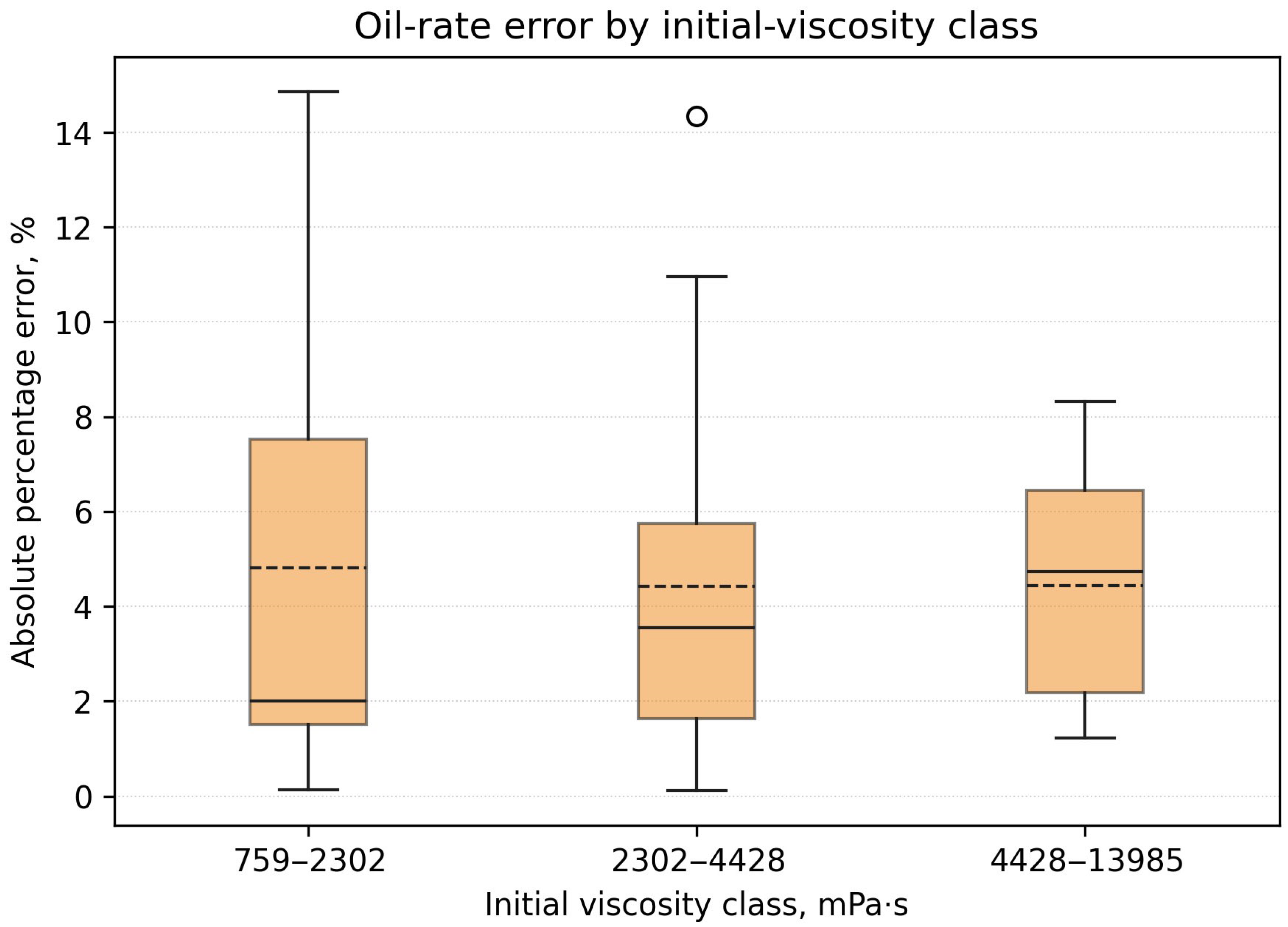
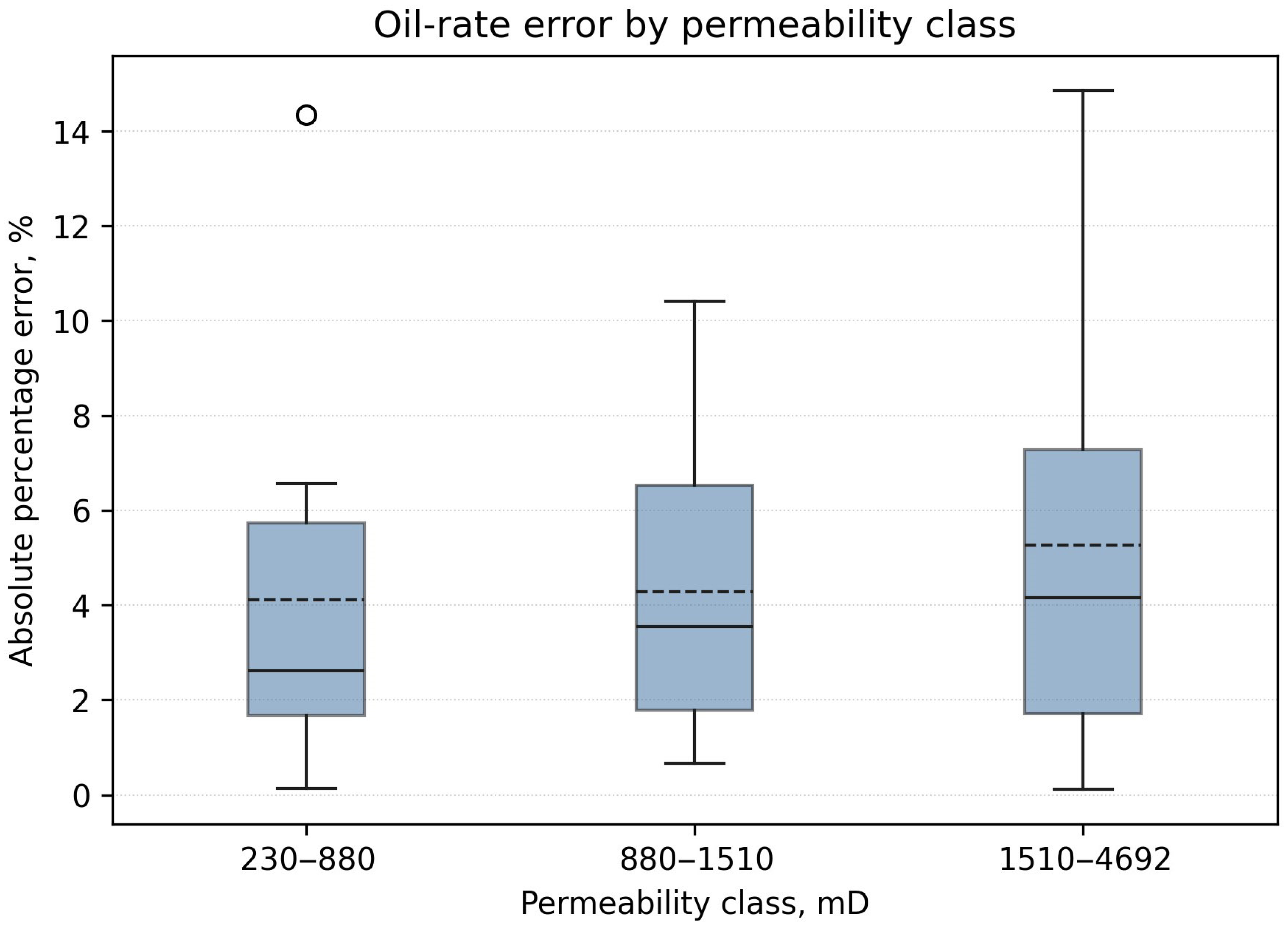
Figure 10 and Figure 11 provide class-wise error checks for two variables that strongly affect transferability: initial oil viscosity and permeability. Error does not collapse in any class, but it increases in the most difficult domains, namely high-viscosity and low-permeability regimes. These regimes should therefore receive priority in future experimental expansion and external validation.

6.5. Production–Steam–Consumption Trade-Off

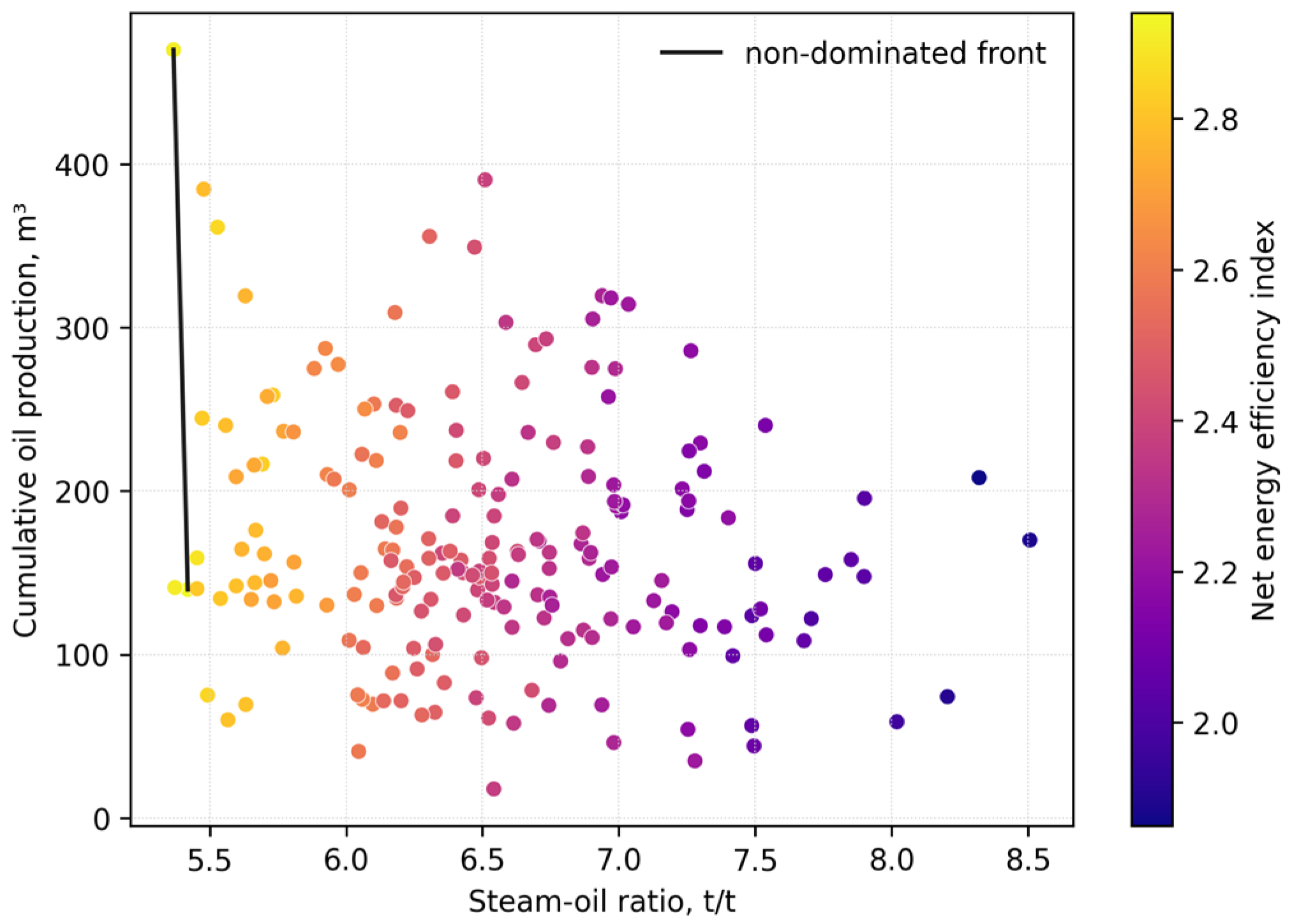
The Pareto analysis in Figure 12 was reformulated as a three-objective dominance problem. A candidate regime was considered non-dominated only if no other admissible regime simultaneously provided higher cumulative oil production, lower SOR and a higher thermal-energy efficiency index. Thus, the thermal-energy efficiency index was incorporated directly into the Pareto-dominance rule rather than being used only as a colour scale. The resulting front separates regimes where additional steam produces a favourable production increase from regimes where steam consumption rises faster than the production and thermal-efficiency benefit.

For two admissible regimes a and b, regime a dominates regime b if

$${\widehat{Q}}_{o,a}\ge {\widehat{Q}}_{o,b}, SO{R}_a\le SO{R}_b, {\widehat{\eta }}_{E,a}^{th}\ge {\widehat{\eta }}_{E,b}^{th},$$

and at least one of the three inequalities is strict. The non-dominated set therefore reflects a simultaneous compromise between production gain, specific steam consumption and thermal-energy efficiency preservation.

7. Validation, Transferability Checks and Ablation Study

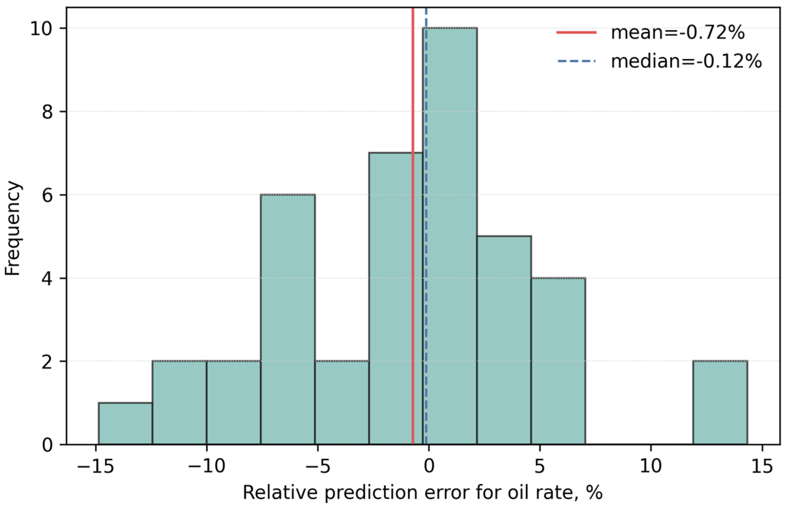
The distribution of blind-test oil-rate errors is shown in Figure 13. Most relative errors are concentrated near zero, and no pronounced one-sided bias is observed. The result supports preliminary engineering screening within the measured operating domain, but it does not justify extrapolation to reservoirs, steam generators or oil compositions outside the ranges represented by the dataset.

7.1. Transferability-Oriented Validation

To test whether the model performance is not limited to a random regime-level split, additional grouped and chronological validation checks were performed. The grouped tests withheld complete operating campaigns, permeability–viscosity classes or available well identifiers from training, while the chronological forward test trained the model on earlier regimes and evaluated it on later regimes. These tests are intentionally more conservative than the main blind-test split because they reduce the probability that campaign-specific or reservoir-state-specific information is shared between the development and validation subsets. However, the dataset does not contain genuinely independent external reservoirs, and well identifiers are incomplete. Therefore, the results in

Table 11. Grouped and chronological robustness checks with fold-level variability.

Validation Mode	Grouping or Test Definition	Number of Groups/Folds	Test Regimes per Fold, Min–Median–Max	Fully Withheld Unit	Oil Rate MAPE, %, Mean ± SD	Cumulative Oil MAPE, %, Mean ± SD	SOR MAPE, %, Mean ± SD	Thermal Efficiency MAPE, %, Mean ± SD	Interpretation
Regime-level blind test	Non-overlapping regime-level split	1 test split	41	Regime records only	4.56	3.86	4.48	3.29	Main blind-test reference; does not test group dependence
Leave-one-campaign-out	Operating campaign withheld	8 folds	18–25–31	Complete operating campaign	5.21 ± 0.62	4.47 ± 0.58	5.36 ± 0.71	4.02 ± 0.49	Tests campaign-related dependence
Permeability–viscosity grouped split	Internally defined class withheld	6 folds	24–33–41	Complete permeability–viscosity class	5.64 ± 0.77	4.83 ± 0.64	5.91 ± 0.83	4.39 ± 0.57	Tests robustness under shifted measured reservoir conditions
Chronological forward test	Later chronological block withheld	1 forward split	46	Later operating block	5.08	4.31	5.22	3.91	Tests forward operational transfer within the measured period
Leave-one-well-available	Available well identifier withheld	11 folds	6–13–19	Complete labelled well subset	5.47 ± 0.81	4.68 ± 0.69	5.74 ± 0.88	4.28 ± 0.61	Availability-based well-level robustness; 54 regimes lack well identifier
External independent reservoir	Not available in present dataset	–	–	No external reservoir withheld	Not claimed	Not claimed	Not claimed	Not claimed	Required for future external transferability validation

are reported as within-dataset grouped robustness checks rather than as proof of external field transferability.

Table 11 shows that the grouped checks produce higher and more variable errors than the main regime-level blind split. This is expected because the model cannot rely on neighbouring regimes from the same campaign, permeability–viscosity class or available well subset. The largest degradation was observed for the permeability–viscosity grouped split, especially for SOR, indicating that steam-consumption indicators are more sensitive to shifted reservoir conditions than direct production responses. The leave-one-well-available test also shows increased fold-level variability, which is consistent with incomplete well identifiers and possible well-related dependence. Therefore, the results support preliminary regime-level screening within the measured domain, but they do not establish transferability to genuinely independent reservoirs or unrelated field conditions.

7.2. Ablation and Benchmark Comparison

An ablation and benchmark study was performed to separate the contributions of the semi-empirical baseline, raw data-driven learning, physically derived features and the complete residual-learning framework. Four model variants were compared on the same blind-test subset: the semi-empirical baseline alone, a purely data-driven gradient-boosting model using leakage-screened raw inputs, a gradient-boosting model using only derived physically interpretable features, and the complete residual-learning framework. 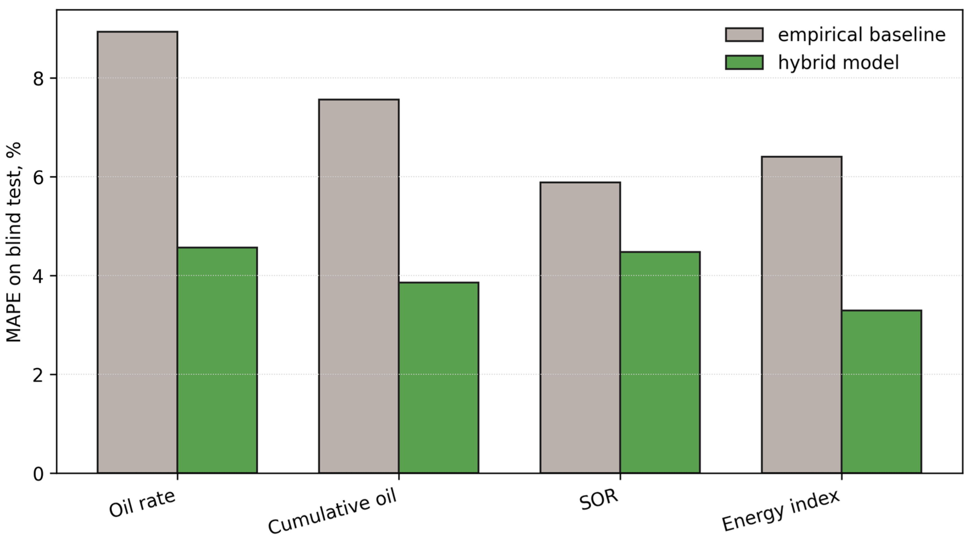Figure 14 summarizes the MAPE values for the four target responses, and

Table 12. Ablation and benchmark comparison on the blind-test subset.

Target Response	Semi-Empirical Baseline-Only MAPE, %	Raw-Input Gradient-Boosting MAPE, %	Derived-Feature Gradient-Boosting MAPE, %	Complete Residual-Learning Framework MAPE, %
Oil production rate	7.84	5.37	5.08	4.56
Cumulative oil production	6.72	4.82	4.39	3.86
SOR	5.54	5.18	4.93	4.48
Thermal-energy efficiency index	5.81	4.31	3.92	3.29

reports the corresponding numerical comparison.

Table 12 gives the numerical MAPE comparison underlying the bar-chart summary in Figure 14.

The ablation results show that each modelling layer contributes to the final accuracy. The semi-empirical baseline alone provides a physically interpretable but less flexible reference response, with MAPE values of 7.84% for oil production rate, 6.72% for cumulative oil production, 5.54% for SOR and 5.81% for the thermal-energy efficiency index. Raw-input gradient boosting reduces the error for direct production responses but remains less stable for composite indicators. The derived-feature gradient-boosting model performs better than the raw-input model for all four targets, confirming that physically interpretable feature construction adds useful information beyond generic nonlinear regression. The complete residual-learning framework gives the lowest MAPE values: 4.56% for oil production rate, 3.86% for cumulative oil production, 4.48% for SOR and 3.29% for the thermal-energy efficiency index. Therefore, the reported improvement is attributable to the combined baseline-plus-residual architecture rather than to model complexity alone.

7.3. Prediction Intervals for Decision-Oriented Regime Screening

Point predictions are insufficient for steam-supply selection because the engineering decision depends not only on expected oil production, but also on the probability of excessive steam consumption. Prediction intervals were therefore added for the four target responses. In the revised procedure, interval widths were estimated only from calibration-subset residuals, while the blind-test subset was used only for out-of-sample coverage evaluation. The blind-test residuals were not used to construct the intervals. Target-specific scaling factors were fitted on the calibration subset to account for increased residual dispersion in high-viscosity and high-cumulative-steam domains. For conservative screening, a candidate regime was accepted only if the lower prediction bound for cumulative oil production exceeded $Q_{\min }$, the upper prediction bound for SOR remained below $SO{R}_{\max }$, and the lower prediction bound for the thermal-energy efficiency index exceeded the minimum admissible thermal-efficiency threshold.

For each target response, the calibration residual quantiles were used to define the prediction interval:

$$P{I}_{m,j}^{(1-\alpha )}=\left[{\widehat{y}}_{m,j}-s_m(z_j)q_{m,1-\alpha /2}^{\mathrm{cal}}, {\widehat{y}}_{m,j}+s_m(z_j)q_{m,1-\alpha /2}^{\mathrm{cal}}\right],$$

where $P{I}_{m,j}^{(1-\alpha )}$ is the $\left(1-\alpha \right)$-level prediction interval for response m and candidate regime j; ${\widehat{y}}_{m,j}$ is the point prediction; $q_{m,1-\alpha /2}^{\mathrm{cal}}$ is the corresponding absolute calibration-residual quantile for target m; and $s_m(z_j)$ is a target-specific scaling factor fitted on the calibration subset as a function of regime descriptor $z_j$. For direct production responses, $s_m(z_j)$ was close to unity. For SOR, it increased in high-viscosity and high-cumulative-steam domains.

For a candidate regime j, the interval-aware acceptance rule was defined as

$$Q_{o,j}^L\ge Q_{\min }, SO{R}_j^U\le SO{R}_{\max }, {({\eta }_{E,j}^{th})}^L\ge {\eta }_{E,\min }^{th},$$

where $Q_{o,j}^L$ is the lower prediction bound for cumulative oil production, $SO{R}_j^U$ is the upper prediction bound for SOR, and ${({\eta }_{E,j}^{th})}^L$ is the lower prediction bound for the thermal-energy efficiency index. Calibration-derived prediction-interval widths and blind-test empirical coverage values are presented in

Table 13. Calibration-derived prediction-interval width and blind-test empirical coverage.

Target Response	Point-Estimate MAPE, %	Mean 80% Interval Width from Calibration Residuals	Mean 95% Interval Width from Calibration Residuals	Blind-Test 80% Coverage, %	Blind-Test 95% Coverage, %	Decision Implication
Oil production rate, m3/day	4.56	0.86 m3/day	1.38 m3/day	80.5	92.7	Direct production response is comparatively stable
Cumulative oil production, m3	3.86	18.4 m3	30.2 m3	78.0	90.2	Suitable for lower-bound production screening, with conservative margin
SOR, t/t	4.48	0.81 t/t	1.28 t/t	73.2	87.8	Requires upper-bound screening due to composite uncertainty
Thermal-energy efficiency index, –	3.29	0.21	0.35	78.0	90.2	Suitable for conservative thermal-efficiency filtering

.

Because the intervals were constructed from calibration residuals and evaluated on the blind-test subset, the reported coverage values are out-of-sample with respect to interval construction. Coverage for oil rate and cumulative oil production remained close to the nominal levels, although slightly conservative deviations were observed. SOR showed lower blind-test coverage because its residual variance increases under high-steam and high-viscosity conditions. For this reason, SOR was treated conservatively in the operating-window selection: regimes close to the SOR_max boundary were not accepted unless the upper prediction bound also satisfied the SOR constraint.

In the final operating-window selection, point-predicted Pareto membership was combined with calibration-derived interval-aware feasibility screening. A regime located on the non-dominated front was retained in the recommended window only if its 95% prediction interval, constructed without using blind-test residuals, satisfied the conservative feasibility rule for cumulative oil, SOR and thermal efficiency. This additional filter reduces the probability of selecting regimes that appear favourable in point estimates but become steam-inefficient under plausible SOR uncertainty. The interval-based Pareto screening should therefore be interpreted as a conservative within-domain decision filter, not as a fully external uncertainty guarantee.

8. Discussion

The study is positioned as experimentally grounded, physics-motivated semi-empirical residual learning rather than as a purely computational forecasting exercise. The central methodological point is that the learning block is structured by an interpretable representation of useful heat delivery, calibrated viscosity reduction, mobility growth and steam consumption. This structure is necessary because steam-assisted heavy-oil production is not a direct regression problem from steam rate to production rate; the response is mediated by heat losses, steam quality, oil rheology, reservoir conductivity and exposure duration.

The measured viscosity–temperature relationship is the strongest physical anchor of the model. It prevents the residual learning unit from treating viscosity as an arbitrary statistical covariate and links the oil-rate response to a well-defined thermal mechanism. The factor-ranking and residual diagnostics support this interpretation: steam rate and quality control heat delivery, while viscosity and permeability determine whether the delivered heat can be converted into increased mobility and production.

The physical baseline was revised to remove two potential inconsistencies identified during review. First, the mobility descriptor was reformulated as a Darcy-consistent ratio in which effective oil viscosity appears in the denominator. Therefore, the descriptor cannot increase when residual oil viscosity remains high. Second, the cumulative-production baseline was reformulated with an explicit saturation multiplier, so longer steam exposure produces diminishing marginal cumulative-production gain rather than unlimited proportional growth. These changes make the baseline more physically interpretable, while preserving its intended role as a semi-empirical engineering approximation rather than a full thermal reservoir simulator.

The leakage-control procedure was also made explicit in the revised manuscript. The model does not use one common predictor matrix for all four responses. Instead, separate feature matrices were defined for oil production rate, cumulative oil production, SOR and the thermal-energy efficiency index. This is especially important for SOR and thermal efficiency, because these indicators can otherwise be reconstructed from cumulative steam, produced oil mass or useful heat input. The revised target-specific predictor table clarifies which measured or derived variables were excluded for each response before training, grouped validation and blind-test evaluation.

The response-surface and uncertainty analyses were also revised to address scale and validation concerns. The cumulative-oil response surfaces were checked against the observed regime-level cumulative-production range before plotting, and the corrected Figure 7 reports cumulative oil in m³ per operating regime within the measured-domain scale. Prediction intervals were reconstructed from calibration-subset residuals, while the blind-test subset was used only for empirical coverage evaluation. Therefore, the interval-based screening no longer uses the same blind-test residuals for both interval construction and interval assessment. Nevertheless, the intervals remain within-domain uncertainty estimates and should not be interpreted as external uncertainty guarantees for unrelated reservoirs.

The revised operating-window analysis also limits causal overinterpretation of the response surface. The steam-rate/steam-quality maps were generated conditionally for representative reservoir-state vectors rather than by pooling heterogeneous regimes with different permeability, thickness, viscosity, saturation and depth. This revision is important because a pooled surface may visually attribute production differences to controllable steam variables while part of the response is actually caused by hidden reservoir-state variation. The three-objective Pareto rule further ensures that thermal efficiency enters the dominance calculation directly, rather than serving only as a descriptive colour variable. From an engineering standpoint, the most useful output is the operating-window analysis. The conditional response maps and three-objective Pareto front show that rational steam supply is formed by a compromise between cumulative production, SOR and the thermal-energy efficiency index. This is more informative than a single maximum-oil-rate recommendation, because thermal EOR often becomes economically and energetically inefficient when additional steam mainly increases heat losses and specific steam consumption. Compared with the benchmark and ablation variants, the complete residual-learning framework provides the most balanced performance across direct production responses and composite steam-efficiency indicators. The ablation study shows that the improvement is associated with the combined use of a semi-empirical baseline, physically interpretable derived features and residual correction. The main gain is therefore methodological rather than merely numerical: production forecasting, steam-consumption assessment and thermal-efficiency screening are treated within a single physically interpretable workflow.

The study has several limitations that define the proper interpretation of the results. First, the conclusions are valid only within the measured ranges of viscosity, permeability, steam quality, injection rate and exposure duration. In addition, the 200 operating regimes are regime-level modelling units rather than 200 fully independent wells or reservoirs. The records are grouped by operating campaign, oil sample, reservoir-state class and available well identifier; therefore, residual within-group dependence cannot be fully excluded. This limitation is addressed through grouped robustness checks, but independent reservoir-scale validation remains necessary before the model can be claimed to transfer to unrelated geological units. Second, SOR and the thermal-energy efficiency index are composite indicators, so their predictive accuracy is naturally lower than the accuracy for oil rate and cumulative production. The revised SOR residual diagnostics show that uncertainty increases in high-SOR, high-viscosity and high-cumulative-steam regimes. Consequently, operating-window selection should rely on interval-aware constraints rather than on point estimates alone. Third, the model is a physics-motivated semi-empirical engineering surrogate and does not replace detailed thermohydrodynamic simulation when spatial heterogeneity, gravity override, capillary effects, chemical alteration of oil or well-pattern interaction must be resolved explicitly. Future work should add external field-scale validation on independent wells, genuinely independent reservoirs and new operating campaigns. Such validation should use fully withheld geological units with complete well identifiers and pre-specified test folds, rather than only internally defined permeability–viscosity classes. This is necessary before the model can be claimed to transfer to unrelated field conditions.

9. Conclusions

An experimental physics-motivated residual-learning framework was developed for forecasting high-viscosity-oil production under steam injection and for selecting thermally rational steam-supply regimes. The dataset used in this study contains 200 regime-level measured records, 4800 steam-injection log entries, 4800 production-response log entries, 360 viscosity–temperature measurements and 60 repeatability/QC records. The 200 regimes were treated as effective modelling units, while possible campaign-, oil-sample-, reservoir-state- and well-related dependence was evaluated through grouped robustness checks rather than assumed absent.

Blind-test validation confirmed stable predictive performance: R² = 0.974 and MAPE = 4.56% for oil production rate; R² = 0.988 and MAPE = 3.86% for cumulative oil production; R² = 0.731 and MAPE = 4.48% for SOR; and R² = 0.828 and MAPE = 3.29% for the thermal-energy efficiency index.

The factor analysis and residual diagnostics show that the production response is controlled by the coupled action of steam rate, steam quality, heat input, exposure duration, initial oil viscosity and permeability. This confirms that the model must retain physical structure and should not be reduced to a purely empirical or black-box mapping. The revised baseline formulation uses a Darcy-consistent mobility descriptor and a saturation-type cumulative-production relation. These corrections ensure that the semi-empirical physical component does not produce monotonic behaviour that contradicts filtration theory or unlimited accumulation with injection duration.

The conditional steam-supply response maps and the three-objective Pareto analysis identify bounded operating regions in which cumulative production gain, SOR and the thermal-energy efficiency index remain balanced for representative reservoir-state classes. The practical role of the model is preliminary engineering screening of steam regimes, identification of excessive steam-consumption cases and prioritization of operating conditions for more detailed thermohydrodynamic analysis or field testing.

The model should not be extrapolated beyond the measured domain without recalibration. The grouped-validation results should be interpreted as within-dataset robustness checks rather than as proof of external transferability to independent reservoirs. The corrected operating-window analysis uses cumulative-oil response surfaces constrained to the observed regime-level production scale. Because SOR and the thermal-energy efficiency index are composite indicators, the revised operating-window procedure uses calibration-derived prediction intervals and conservative feasibility checks rather than point estimates alone. Future work should extend the dataset using additional field-scale regimes, complete well identifiers, fully withheld independent reservoirs, explicit post-intervention validation and a more detailed uncertainty model for SOR and thermal-efficiency indicators.