FFT-Free Neural Operators for Helmholtz Scattering via Adaptive Coefficient Modulation

Featured Application

The proposed Helmholtz Neural Operator is a candidate fast-forward surrogate for the low-to-moderate-frequency forward maps inside many-query workflows such as seismic full-waveform inversion, parametric uncertainty quantification of heterogeneous media, and real-time medical-ultrasound or non-destructive-evaluation imaging pipelines; field-scale high-frequency and closed-loop inverse uses remain to be validated.

Abstract

Fourier Neural Operators (FNOs) exhibit mode saturation on high-contrast inhomogeneous media, and recent multi-scale extensions (MscaleFNO) further worsen out-of-distribution (OOD) generalization. We introduce the Helmholtz Neural Operator (HNO), a physics-informed, FFT-free branch–trunk operator in the DeepONet family, with a hybrid SIREN+learnable-Fourier trunk and a dual-path rank-32 hypernetwork branch, with bounded multiplicative gating on per-mode coefficients. At a matched parameter count (∼1.05 M, five seeds), HNO achieves a 2.6× lower OOD generalization gap than FNO (19.6% vs. 50.6%, $p=1.7\times {10}^{-3}$, Cohen’s $d=5.1$), 5.1× lower than vanilla DeepONet (19.6% vs. 99.9%, $p=8.2\times {10}^{-3}$), and 6.0× lower than MscaleFNO (19.6% vs. 117.4%, $p=2.4\times {10}^{-6}$); MscaleFNO’s deficit grows at 4.2× more parameters, ruling out capacity starvation. HNO is 4.6×/16.4× faster than FNO/MscaleFNO and 64×–245× faster than multi-threaded FD-PML (MKL PARDISO, 12 cores; 183×–698× vs. single-thread scipy.spsolve), making it suitable as a forward surrogate inside many-query workflows. Absolute accuracy on extreme-contrast (15:1) OOD samples is limited (relative $L^2\approx 1$), so HNO is positioned as a many-query surrogate or warm start for refinement loops, not a stand-alone replacement for direct solvers. A scope limitation is that HNO underperforms FNO on elliptic Darcy Flow, confirming specialization for hyperbolic/wave equations rather than universal operator learning.

1. Introduction

Wave scattering in inhomogeneous media is a recurring computational task across applied science and engineering: seismic imaging and full-waveform inversion in geophysics, non-destructive evaluation of composite materials, underwater acoustics for sonar, and medical ultrasound imaging, among others. Classical numerical treatments—finite differences, finite elements, boundary elements, and Perfectly Matched Layer (PML) truncations—deliver controlled accuracy but must be repeatedly invoked for parametrically varying media, motivating interest in learned surrogate solvers that amortize the forward-map cost across design studies, inverse problems, and real-time applications.

Neural operators have emerged as a promising class of such surrogates, learning mappings directly between infinite-dimensional function spaces [1,2,3]. Among these, the Fourier Neural Operator (FNO) [1] attains computational efficiency through spectral convolutions, leveraging the Fast Fourier Transform (FFT) for global receptive fields with quasi-linear complexity. However, a fundamental limitation emerges when applying FNO to inhomogeneous media—materials with spatially varying properties that induce sharp gradients or effective discontinuities in solution fields. This inhomogeneous-media regime is precisely the one of practical engineering interest.

1.1. The Mode Saturation Problem

Consider the 2D Helmholtz equation governing wave propagation in heterogeneous media:

$${\nabla }^{2}u\left(\mathit{x}\right)+k_0^2{n}^2\left(\mathit{x}\right)u\left(\mathit{x}\right)=f\left(\mathit{x}\right),\mathit{x}\in \mathsf{\Omega }\subset {\mathbb{R}}^2$$

(1)

where $n^2\left(\mathit{x}\right)$ is the refractive index distribution. When $n^2$ exhibits high spatial contrast (e.g., a 15:1 ratio), fixed Fourier bases exhibit mode saturation—additional modes provide diminishing returns even in regions far from material interfaces. Our experiments confirm that scaling FNO from 4 to 6 modes yields no improvement in OOD generalization despite having $2.2\times$ more parameters (

Table 1. Comparison on Helmholtz scattering. Parameter-matched (∼1.05 M) comparison forms the primary fair evaluation: HNO achieves 2.6× better generalization than FNO, 5.1× better than vanilla DeepONet, and 6.0× better than MscaleFNO. The DeepONet row probes the structural family HNO sits inside (Section 2.3, “Relation to DeepONet”): a generic branch–trunk operator without our hybrid SIREN+Fourier trunk and without the bounded factored branch fails on this problem at matched capacity. To rule out per-branch capacity starvation, we additionally evaluate MscaleFNO at its original per-branch configuration (width 64, 4.40 M total); OOD gap worsens to 148.0%, confirming the architectural (not capacity) limitation. Train Loss is the relative $L^2$ on the training set at the best-val checkpoint; comparing Train, InD, and OOD columns reveals where each architecture’s gap comes from. All results are averaged over 5 seeds; ± indicates standard deviation. Bold marks the proposed HNO reference row, which attains the best (lowest) train loss, OOD loss, generalization gap, and inference time.

Model	Params	Train Loss	InD Loss	OOD Loss	Gen Gap	Inf. (ms)
FNO variants (non-matched parameter budgets)
FNO-4m (baseline)	550 K	—	0.880 ± 0.004	1.223 ± 0.046	39.0 ± 5.6%	10.1
FNO-4m7L	955 K	—	0.870 ± 0.005	1.218 ± 0.041	40.1 ± 5.1%	17.1
FNO-6m4L	1205 K	—	0.861 ± 0.002	1.340 ± 0.068	55.6 ± 8.1%	10.2
Parameter-matched comparison (∼1.05 M params each)
DeepONet ‡	1046 K	0.919 ± 0.010	0.922 ± 0.002	1.843 ± 0.340	99.9 ± 36.9%	4.02 ± 0.01
FNO-5m5L	1054 K	0.859 ± 0.005	0.860 ± 0.002	1.296 ± 0.075	50.6 ± 8.6%	13.98 ± 0.02
MscaleFNO-N8	1052 K	0.855 ± 0.002	0.865 ± 0.002	1.880 ± 0.048	117.4 ± 5.6%	50.48 ± 0.04
HNO (Ours)	1047 K	0.831 ± 0.020	0.866 ± 0.004	1.036 ± 0.014	19.6 ± 1.1%	3.05 ± 0.00
Capacity-unmatched: MscaleFNO with 4.2× more parameters (per-branch width 64)
MscaleFNO-N8-wide †	4398 K	—	0.867 ± 0.001	2.150 ± 0.215	148.0 ± 24.8%	90.55 ± 0.75

^‡ Vanilla DeepONet [2] at matched capacity (branch CNN 32–64–128–256, trunk MLP with $K_{\mathrm{F}}$ = 64 Fourier features, $4\times 256$ hidden, p = 128 basis functions); the high training loss (≈0.92) indicates the generic trunk basis cannot fit Helmholtz solutions even within distribution. ^† Trained at batch size 16 (vs. 32 for all others): the 4.40 M-parameter configuration peaks at 16.8 GiB, exceeding consumer-GPU capacity (12 GiB RTX 3060) at batch 32. This deployability gap is itself informative—MscaleFNO requires specialized hardware to run at standard batch sizes, while HNO fits in 1.5 GiB.

).

1.2. Theoretical Motivation

Kolmogorov n-width theory [4] provides a rigorous framework for understanding this limitation. For solution manifolds arising from piecewise constant media, the effective dimensionality scales unfavorably with contrast ratio. While smooth solutions admit exponential decay $d_n\sim e^{-c{n}^{1/d}}$, discontinuous solutions decay only as $d_n\sim n^{-1/2}$ [5]. This suggests that adaptive bases—which adjust to input structure—could achieve better approximation rates.

1.3. Prior Attempts: Spectral Capacity Scaling

A natural response to mode saturation is to increase spectral capacity. MscaleFNO [6] partitions the input into frequency-scaled sub-networks and aggregates their outputs, inspired by multi-scale deep neural networks [7]. While this improves in-distribution fitting, our controlled experiments (Section 3.1) show that such capacity scaling worsens OOD generalization: MscaleFNO attains a 117.4% gap versus FNO’s 50.6% and HNO’s 19.6% at matched parameters, and the gap widens further to 148.0% when MscaleFNO is given 4.2× more parameters (4.40 M). The degradation is monotonic in branch capacity, consistent with parallel branches progressively overfitting the training distribution.

1.4. Contribution: Helmholtz Neural Operator

We propose the Helmholtz Neural Operator (HNO), an FFT-free branch–trunk operator that sits formally within the DeepONet family [2] (made precise in Section 2.3). Its contribution is not the branch–trunk separation itself—which DeepONet already provides—but two design choices within that family, tailored to high-contrast wave scattering: (i) a hybrid SIREN+learnable-Fourier trunk that fixes a basis combining local smoothness and global periodicity, and (ii) a factored branch that makes the per-mode coefficients medium-dependent. The essential element of (ii) is that the per-mode coefficients are input-conditioned on the medium; we realize this as a bounded multiplicative gate, but ablations across additive FiLM, attention, dynamic routing, and even removing the gate entirely (Section 3.4) all perform comparably, so the gate is a deliberately generic, accuracy-neutral robustness mechanism, and the wave-tailored hybrid trunk (i) is the empirically load-bearing choice. We retain the bounded gate as a stable, safety-bounded default. Specifically, these choices are realized by the following components:

• HybridBasisNetwork: SIREN [8] backbone with learnable Fourier frequencies, providing both local smoothness (SIREN) and global periodicity (Fourier).
• EnhancedModulator: A rank-32 LoRA-style [9] hypernetwork that computes per-mode coefficient modulations from encoded input media.
• SpatialFeatureEncoder: A nonlinear feature extractor (here instantiated as a multi-scale CNN producing a multi-scale spatial feature tensor and a pooled context vector) that supplies the modulator with input-dependent context. As we show in Section 3.4, the controlling factor is that the encoder is nonlinear; a linear projection collapses, but CNN and MLP encoders are largely interchangeable at matched capacity.

The key insight is that the operator should adapt to the input medium’s contrast structure by re-weighting a fixed, wave-tailored basis for each input medium, placing the input dependence in the branch coefficients rather than in the basis functions,  in contrast to approaches that merely increase the number of fixed spectral modes.

Through rigorous parameter-matched experiments with five random seeds, we demonstrate that the system

• Has 2.6× better OOD generalization than FNO: 19.6 ± 1.1% vs. 50.6 ± 8.6% gap ($p=1.7\times {10}^{-3}$);
• Is 5.1× better than vanilla DeepONet at matched parameters: 19.6% vs. 99.9 ± 36.9% gap ($p=8.2\times {10}^{-3}$); a modulation-presence ablation (Section 3.4) attributes this gain to the hybrid SIREN+Fourier trunk, the coefficient modulation being accuracy-neutral within the branch–trunk family;
• Has 6.0× better OOD generalization than MscaleFNO at matched parameters: 19.6% vs. 117.4 ± 5.6% gap ($p=2.4\times {10}^{-6}$);
• Is 7.6× better than MscaleFNO even at 4.2× more parameters: 19.6% vs. 148.0 ± 24.8% gap ($p=3.2\times {10}^{-4}$); the OOD gap worsens monotonically with branch capacity;
• Is 4.6× faster than FNO, 16.4× faster than MscaleFNO, and 29.6× faster than MscaleFNO-wide: 3.06 ms vs. 13.93 ms vs. 50.26 ms vs. 90.55 ms (FFT-free);
• Is 1.8× more robust to frequency shift over the tested $k_0\in [10,30]$ band: 29.9% vs. 55.2% average gap across $k_0$ variations (see Section 3.3 for the sweep and Section 4.2 for the wavenumber-range caveat);
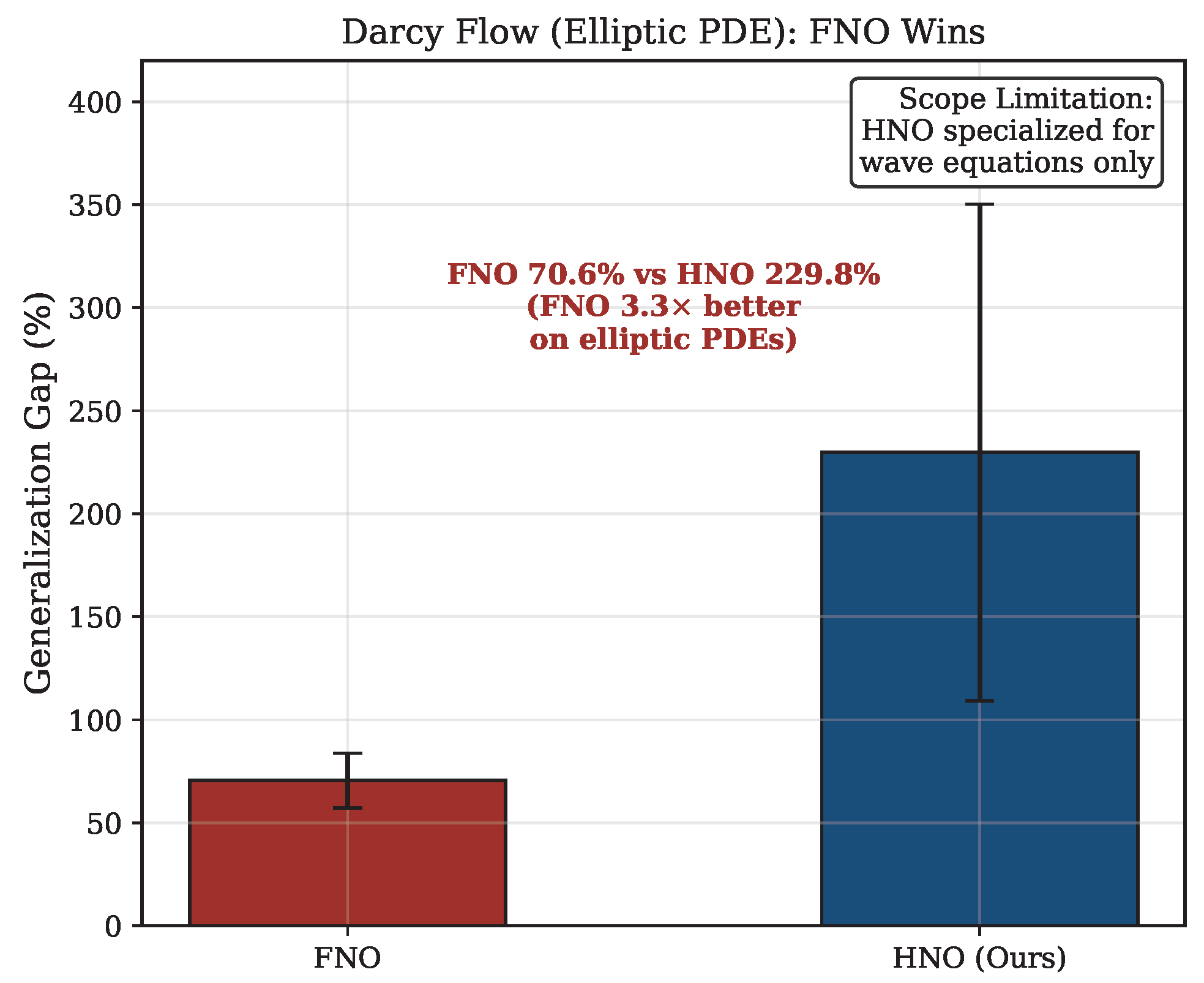
• Scope limitation: HNO underperforms on Darcy Flow (229.8% vs. 70.6% gap), confirming specialization for hyperbolic/wave problems rather than elliptic PDEs.

1.5. Related Work

1.5.1. Neural Operators

Neural operators learn mappings between infinite-dimensional function spaces. DeepONet [2] uses separate branch and trunk networks based on the universal approximation theorem for operators, predicting the solution as $u\left(\mathit{x}\right)={\sum }_k{b}_k\left(\mathrm{input}\right)·t_k\left(\mathit{x}\right)$ via input-dependent coefficients on a coordinate-only trunk basis. FNO [1] instead performs spectral convolutions via FFT, achieving strong performance on fluid dynamics benchmarks. Extensions include Wavelet Neural Operators [10] for multi-scale problems, Geo-FNO [11] for irregular geometries, and GINO [12] for graph-based domains. We do not evaluate Geo-FNO or GINO directly: both target irregular computational domains (deformed meshes and graph-structured point clouds, respectively). On the regular 128 × 128 Cartesian grid used throughout this study, their geometry-handling machinery—coordinate deformation in Geo-FNO, graph–kernel integration in GINO—reduces to the same uniform-grid spectral convolution as standard FNO. We therefore take FNO as the representative fixed-spectral baseline for this regular-grid setting and leave extension to irregular domains as future work (Section 4.2). As we make explicit in Section 2.3, the architecture we propose is formally a DeepONet-family operator with two distinguishing design choices—a hybrid SIREN+learnable-Fourier trunk and a factored, bounded branch parameterization—rather than a separate operator family.

1.5.2. Multi-Scale and Mode-Scaling FNO Variants

A parallel line of work addresses high-frequency and multi-scale PDEs by increasing spectral capacity. MscaleDNN [7] first proposed partitioning input features into frequency-scaled sub-networks to overcome the spectral bias of ReLU networks on oscillatory targets. MscaleFNO [6] extends this idea to neural operators, running N parallel FNO branches on frequency-rescaled inputs and aggregating via learned weights. While effective for reducing in-distribution error on oscillatory function spaces, we demonstrate empirically (Table 1) that this multi-branch spectral scaling degrades OOD generalization at matched parameter count—the N = 8 branches collectively overfit the training distribution, yielding a 117.4% generalization gap compared with 50.6% for vanilla FNO. This degradation is monotonic in branch capacity: expanding per-branch width from 31 to 64 (raising total parameters from 1.05 M to 4.40 M, consistent with the original paper’s recommended per-branch configuration) further worsens the gap to 148.0%, ruling out the hypothesis that the matched-budget underperformance was an artifact of per-branch capacity starvation.

1.5.3. Concurrent Hybrid Architectures for Wave Scattering

Balaji et al. [13] independently identified high-contrast wave scattering as a failure mode of vanilla FNO and proposed a Hybrid FNO–ViT operator: an FNO first encodes a smooth background propagation into feature tokens, which are then passed to a vision transformer that learns high-contrast scattering correction via attention. Their work shares the problem setting with ours (high-frequency Helmholtz with strong contrasts, motivated by seismic imaging) but differs in three substantive ways that position our contribution as complementary rather than redundant:

• FFT dependence. Balaji et al. [13] retain the FNO as the background-propagation stage and stack a transformer on top; the spectral convolution (and hence the FFT) remains the computational core. Our architecture is FFT-free: spectral behavior is captured by a small set of learnable Fourier frequencies inside HybridBasisNetwork rather than by a global transform. This yields a 4.6× wall-clock speedup over FNO at a matched parameter count (Section 3.1).
• What is being learned. Balaji et al. learn a two-stage decomposition (smooth + correction) with attention modeling long-range scattering. We instead learn a single unified adaptive operator: a medium-conditioned hypernetwork re-weights the per-mode coefficients of a fixed hybrid basis so that the same operator becomes locally smooth in homogeneous regions and locally discontinuity-aware near interfaces. The mechanism is architectural conditioning, not explicit residual decomposition.
• Evaluation focus. Balaji et al. [13] report in-distribution phase/amplitude accuracy and accuracy–parameter scaling. Our study is centered on out-of-distribution generalization across complexity levels and wavenumbers, with paired-seed statistical tests (Cohen’s $d=5.1$, $p=1.7\times {10}^{-3}$). We further report a negative result on Darcy Flow (Section 4.1), delineating the scope of our claims.

These differences motivate our framing of HNO as an FFT-free, branch–trunk operator with bounded multiplicative gating on per-mode coefficients (cf. Section 2.3), rather than as another hybrid stack built on top of spectral convolutions. A head-to-head experimental comparison against Balaji et al. [13] would require their trained models or a faithful reimplementation; to the best of our knowledge, no public code or data release is available for that method at the time of writing, and reimplementing an attention-based two-stage architecture from the paper description alone would risk misrepresenting it. We therefore restrict the comparison to the conceptual differentiation above and will carry out a direct empirical comparison if and when their implementation becomes available.

1.5.4. Building Blocks: Implicit Representations, Hypernetworks, and Adaptive Bases

HNO’s two design choices draw on three previously separate lines of work, which we summarize together because the architecture’s novelty lies in how they are combined rather than in any one of them. (i) Implicit neural representations supply the trunk: SIREN [8] uses periodic activations to represent high-frequency signals, NeRF [14] popularized coordinate-based networks, and random/learnable Fourier features [15] improve their expressivity. Our hybrid trunk fuses SIREN smoothness with learnable Fourier frequencies. (ii) Hypernetworks and conditional computation supply the branch: hypernetworks [16] generate input-conditioned weights, LoRA [9] introduce low-rank weight updates, and FiLM [17] applies feature-wise modulation; we use a LoRA-style low-rank bottleneck to emit a bounded per-mode multiplicative gate on the branch coefficients. (iii) The classical adaptive-representation tradition motivates the goal: wavelets [18], curvelets [19], and learned dictionaries [20] build representations suited to discontinuous functions, and learned Green’s function operators [21] pursue PDE-specific bases. HNO inherits this tradition’s objective—an input-adapted representation for the discontinuity-rich solutions of high-contrast scattering—but realizes it differently from all three: rather than swapping in a new fixed basis family or synthesizing new basis functions per input, it re-weights a fixed hybrid basis through input-conditioned coefficients. Specifically, the hypernetwork modulates the branch’s coefficient on each (fixed) trunk basis function; it does not modulate the basis functions themselves.

1.5.5. Wavelet Neural Operator and HNO: A Contrast

Of the existing fixed-basis alternatives, the Wavelet Neural Operator (WNO) [10] is the closest in spirit to our work: it replaces FNO’s Fourier convolutions with a discrete wavelet transform, motivated by wavelets’ superior approximation of locally non-smooth functions. Both WNO and HNO target the same failure mode of FNO—fixed Fourier bases requiring many modes to resolve sharp interfaces—but the two answers are structurally different. WNO retains a fixed, data-independent basis: the wavelet family (e.g., Daubechies) is chosen up-front, and the network learns coefficients on that basis via a forward and inverse transform per layer. HNO, by contrast, keeps the basis fixed but makes the per-mode coefficients input-conditioned: a hypernetwork reads the medium $n^2\left(\mathit{x}\right)$ and emits a per-sample multiplicative gate $\Delta \varphi \left(n^2\right)$ that re-weights the $K=64$ fixed basis modes (Equation (7)). Practically, this means WNO commits to a single localization scale ahead of time (the chosen mother wavelet), whereas HNO can shift its effective localization on a per-medium basis at inference. Empirically, curvelets are not evaluated on the high-contrast Helmholtz benchmark we use here; the WNO head-to-head, by contrast, is carried out under our PML/$k_0=20$ protocol in Section 3.2 (

Table 2. Operator head-to-head under the identical PML/$k_0=20$ high-contrast protocol (train Level 3, OOD Level 4), with 3 seeds (vs. 5 for the main comparison). WNO is a db4 (Daubechies-4) wavelet, parameter-comparable operator (∼1.04 M, not exactly matched). Mean ± std.

Model	Params	In-Dist	OOD	Gen. Gap (%)	Infer. (ms)
HNO	1,047,440	0.864	1.036	$+19.9\pm 1.2$	3.11
FNO-5m5L	1,053,634	0.862	1.306	$+51.6\pm 11.8$	13.88
WNO	1,042,306	0.914	1.051	$+15.0\pm 2.5$	44.53

). We position HNO as orthogonal to WNO: it will “learn to reweight a fixed basis” rather than “swap the basis family.”

2. Materials and Methods

2.1. Problem Formulation

We consider the Helmholtz equation (Equation (1)) with Sommerfeld radiation conditions, implemented via Perfectly Matched Layers (PMLs). The goal is to learn the solution operator $\mathcal{G}:n^2\mapsto u$ mapping refractive index distributions to wave fields.

The training data consists of pairs ${\left\{(n_i^2,u_i)\right\}}_{i=1}^N$ generated by a finite-difference solver on a $128\times 128$ grid. We train on “in-distribution” samples and evaluate on “out-of-distribution” samples with different complexity levels or wavenumbers.

2.2. Motivation: Why Input-Adapted Coefficients Are Used for High-Contrast Media

The mode-saturation behavior observed in Section 1 admits a natural interpretation through Kolmogorov n-width theory. Recall the n-width of a compact set K in a Banach space X,

$$d_n\left(K\right)=\underset{\begin{array}{c}{V}_n\subset X\\ \dim \left(V_n\right)=n\end{array}}{\inf }\underset{f\in K}{\sup }\underset{g\in V_n}{\inf }{\parallel f-g\parallel }_X,$$

(2)

which measures the best n-dimensional linear approximation rate over K. For solution manifolds of elliptic operators with smooth coefficients, classical results give exponential decay $d_n\sim e^{-c{n}^{1/d}}$ [4]; for piecewise-smooth functions with discontinuities, the rate degrades to $d_n\sim n^{-1/2}$ [5]. Helmholtz solutions on high-contrast media fall into the second regime: the wave field is smooth in homogeneous subdomains but exhibits effective discontinuities (jumps in normal derivative) at material interfaces. This slow decay is, moreover, characteristic of wave problems in general: for wave- and transport-dominated equations, the linear Kolmogorov n-width is known to decay at best algebraically rather than exponentially [22], a barrier that no choice of fixed linear basis—Fourier or otherwise—can circumvent, and which motivates input-adaptive alternatives specifically for the hyperbolic regime that HNO targets.

This regime is precisely where nonlinear (input-adapted) approximation can outperform any fixed linear n-dimensional subspace. Intuitively, an input-adapted approximation that concentrates its degrees of freedom near the interfaces of a specific medium can outperform a fixed Fourier basis, which must otherwise spend modes uniformly across the spectrum to resolve any interface that could appear. The HNO architecture (Section 2.3) pursues this advantage not by varying the trunk basis functions themselves—which remain fixed and shared across all inputs—but by making the per-mode coefficients a function of the input through a low-rank hypernetwork, reweighting that fixed hybrid basis. Because this is a per-sample reconstruction within a fixed K-dimensional span, the relevant separation is the nonlinear (manifold) width of the medium-to-solution map across inputs rather than the linear n-width of any single sample, so we do not claim HNO formally attains the nonlinear-width rate. We do not prove a quantitative n-width bound for this construction, and we treat the gain as an empirical hypothesis: if input adaptation truly helps, the architecture’s OOD generalization gap should be markedly smaller than that of fixed-basis FNO at a matched parameter count, and ablating the adaptive components should remove the advantage. Section 3.1 and Section 3.4 test exactly these predictions.

• Why a bounded gate aids out-of-distribution behavior.

The argument above motivates adaptivity; the boundedness of the gate plays a separate, complementary role, for which we can give a mechanistic—qualitative, and partially quantitative by construction—account. Because the multiplicative gate satisfies $\Delta {\varphi }_k\in [-\frac{1}{2},\frac{1}{2}]$ for every mode k and every input (Section 2.3), the medium-conditioned coefficient ${\beta }_k={\alpha }_k(1+\Delta {\varphi }_k)$ obeys $|{\beta }_k/{\alpha }_k-1|\le \frac{1}{2}$ uniformly—including on out-of-distribution media arbitrarily far from the training set. The branch therefore cannot answer an unfamiliar medium with an unbounded coefficient excursion: each mode’s relative deviation from the learned in-distribution baseline ${\alpha }_k$ is capped at $50\%$ regardless of the magnitude of the test-time shift, so the worst-case amplification of a distribution shift through the coefficient path is bounded a priori rather than left to be controlled by the training data alone. Extrapolation is thereby confined to a multiplicative band $[\frac{1}{2}{\alpha }_k,\frac{3}{2}{\alpha }_k]$ around the in-distribution coefficients—a guard that an unconstrained branch does not possess. We stress that this is a stability statement, not an approximation-theoretic guarantee: it bounds how far the operator may move under a shift, not how small the resulting error must be, and it does not by itself prove that the bounded model attains lower OOD error than an unbounded one. Empirically, however, the gate-range sweep that isolates boundedness (Section 3.4) shows that OOD performance is insensitive to the bound: the $[-0.3,0.3]$, $[-0.5,0.5]$, $[-0.7,0.7]$, and unbounded variants all overlap within seed noise (unbounded $18.9\%$ vs. bounded $21.0\%$). The bound is therefore best understood as a stability and safety property—an a priori guard against coefficient blow-up on out-of-distribution media—and a stable default, rather than as the empirical driver of the OOD gap; we retain $[-0.5,0.5]$ on that basis. A quantitative bound coupling the gate range to the OOD generalization gap remains open (Section 4.2).

2.3. Helmholtz Neural Operator Architecture

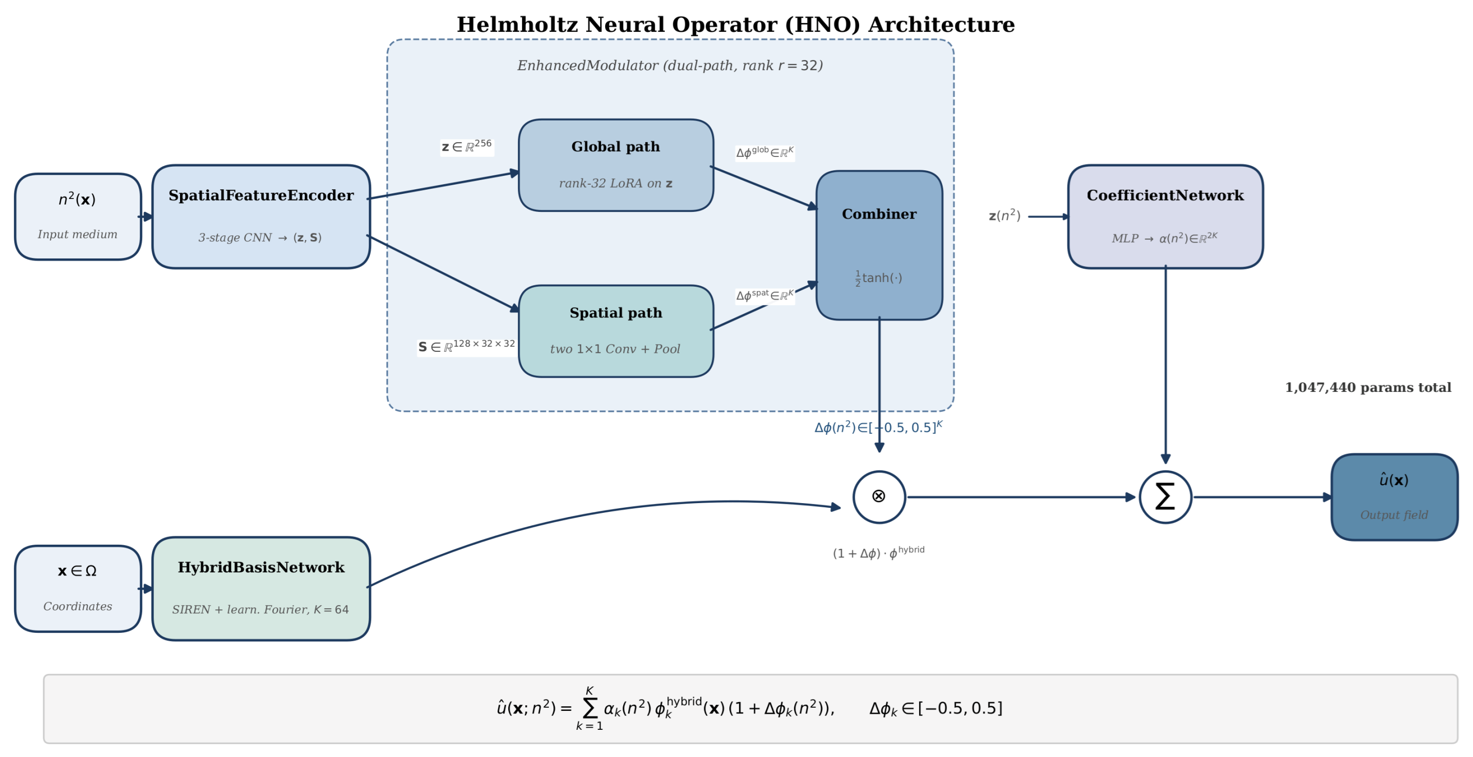
Our architecture (Figure 1) consists of four components totaling 1,047,440 parameters; the wave-equation specialization that motivates the design is documented in Section 4.2. Throughout, we use the term FFT-free in a precise sense: no global Fast Fourier Transform is computed at training or inference time, and the spatial map $n^2\left(\mathit{x}\right)\mapsto \widehat{u}\left(\mathit{x}\right)$ contains no spectral transform layer. The architecture is not “Fourier-free”—a small set of $K_F=16$ learnable Fourier frequencies appears as one component of the basis functions ${\varphi }_k^{\mathrm{hybrid}}\left(\mathit{x}\right)$, but these are evaluated pointwise at coordinates $\mathit{x}$ rather than via a transform of the input. Concretely, the distinction is between a learnable Fourier frequency—a fixed-form sinusoid pair $[\sin ({\mathit{\omega }}_j·\mathit{x}),\cos ({\mathit{\omega }}_j·\mathit{x})]$ with trainable ${\mathit{\omega }}_j$, evaluated at each coordinate $\mathit{x}$ exactly like any other coordinate feature—and a fixed Fourier basis applied through a global transform, as in FNO’s spectral convolution, which forms the discrete Fourier transform of the input field and reweights its modes; only the latter requires an FFT, and HNO uses solely the former.

• HybridBasisNetwork ($K=64$ outputs).

Combines a SIREN backbone with learnable Fourier features:

$${\varphi }^{\mathrm{hybrid}}\left(\mathit{x}\right)=\mathrm{LayerNorm}\left[{\varphi }^{\mathrm{SIREN}}\left(\mathit{x}\right)\oplus {\varphi }^{\mathrm{Fourier}}\left(\mathit{x}\right)\right]\in {\mathbb{R}}^K$$

(3)

where ${\varphi }^{\mathrm{SIREN}}$ is a 3-layer SIREN (128 hidden units, ${\omega }_0=30$), and ${\varphi }^{\mathrm{Fourier}}$ uses 16 learnable frequencies. The concatenation provides both local smoothness (SIREN) and global periodicity (Fourier).

• SpatialFeatureEncoder.

A nonlinear feature extractor that maps the input medium $n^2\left(\mathit{x}\right)$ to two complementary representations consumed by the dual-path modulator below. We instantiate it as a multi-scale CNN with three convolutional stages (channels: $32\to 64\to 128$; two $3\times 3$ convolutions per stage with downsampling between stages). The encoder exposes (i) a pre-pool spatial feature tensor $\mathit{S}\left(n^2\right)\in {\mathbb{R}}^{128\times 32\times 32}$ from the final CNN stage, which retains local structure within the receptive field and is consumed by the spatial path of the modulator, and (ii) a globally aggregated context vector $\mathit{z}\left(n^2\right)\in {\mathbb{R}}^{256}$ obtained by adaptive average pooling of the final feature map to $4\times 4$ followed by a linear projection, which is consumed by the global LoRA path of the modulator. Section 3.4 shows that this CNN choice is not load-bearing—an MLP encoder of matched parameter count performs comparably (slightly better in our simplified-backbone ablation), while a linear-only encoder collapses. The component should therefore be read as “some nonlinear encoder” rather than “CNN specifically.”

• EnhancedModulator (dual-path, rank-32).

The modulator produces a per-mode multiplicative gate $\Delta \varphi \left(n^2\right)\in {[-0.5,0.5]}^K$ by combining two complementary input pathways into a single bounded output. The encoder $\mathcal{E}\left(n^2\right)$ exposes both a multi-scale spatial feature map $\mathit{S}\left(n^2\right)\in {\mathbb{R}}^{C\times H^{\prime }\times W^{\prime }}$ (here $C=128$, $H^{\prime }=W^{\prime }=32$) and a globally aggregated feature vector $\mathit{z}\left(n^2\right)\in {\mathbb{R}}^{256}$.

• Global path (rank-32 LoRA bottleneck): A low-rank bottleneck operates on $\mathit{z}$,

  $$\Delta {\varphi }^{\mathrm{glob}}\left(n^2\right)=W_{\mathrm{up}}^g\mathrm{GELU}\left(W_{\mathrm{down}}^g\mathit{z}\left(n^2\right)\right),$$

  (4)

  with $W_{\mathrm{down}}^g\in {\mathbb{R}}^{2r\times 256}$ and $W_{\mathrm{up}}^g\in {\mathbb{R}}^{K\times 2r}$, where $r=32$ is the rank parameter; the activation between the bottleneck pair is GELU rather than tanh, with the final bounding applied only after the combiner below.
• Spatial path (1 × 1 convolutions + spatial pool): Two $1\times 1$ convolutions process the spatial feature map, and the result is pooled along $H^{\prime }\times W^{\prime }$,

  $$\Delta {\varphi }^{\mathrm{spat}}\left(n^2\right)={\mathrm{Pool}}_{H^{\prime }{W}^{\prime }}\left({\mathrm{Conv}}_{1\times 1}^{\left(2\right)}\left(\mathrm{GELU}\left({\mathrm{Conv}}_{1\times 1}^{\left(1\right)}\left(\mathit{S}\left(n^2\right)\right)\right)\right)\right)\in {\mathbb{R}}^K.$$

  (5)

  The spatial path provides the modulator with information that retains local structure within the encoder’s receptive field, in contrast to the globally averaged $\mathit{z}$.
• Combiner (bounded gate): the two paths are concatenated and projected through a tanh-bounded linear layer,

  $$\Delta \varphi \left(n^2\right)=\frac{1}{2}\tanh \left(W_c\left[\Delta {\varphi }^{\mathrm{glob}}\left(n^2\right);\Delta {\varphi }^{\mathrm{spat}}\left(n^2\right)\right]+{\mathit{b}}_c\right)\in {[-0.5,0.5]}^K,$$

  (6)

  where $W_c\in {\mathbb{R}}^{K\times 2K}$.

The tanh bound combined with the $\frac{1}{2}$ scaling enforces $\Delta {\varphi }_k\in [-0.5,0.5]$, which constrains the effective branch coefficient ${\beta }_k={\alpha }_k(1+\Delta {\varphi }_k)$ to the interval $[0.5{\alpha }_k,1.5{\alpha }_k]$ (cf. Equation (8)). The dual-path structure is a robustness refinement rather than the load-bearing component: the path-decomposition ablation (Section 3.4) shows that the global LoRA path alone already attains a 20.4% gap, statistically indistinguishable from the full dual path (21.0%). As we show in Section 3.4, the OOD advantage is traced primarily to the hybrid trunk and an adequately sized modulator, while the spatial path, the encoder structure (CNN vs. MLP), and the gate bound are comparatively minor at matched capacity.

• CoefficientNetwork.

An MLP predicts expansion coefficients $\alpha \left(n^2\right)\in {\mathbb{R}}^{2K}$ (real and imaginary parts).

• Output Reconstruction.

The final prediction reconstructs the wave field from the fixed basis functions, the per-mode coefficients, and the bounded multiplicative gates:

$$\widehat{u}(\mathit{x};n^2)={\displaystyle \sum _{k=1}^K}{\alpha }_k\left(n^2\right)·{\varphi }_k^{\mathrm{hybrid}}\left(\mathit{x}\right)·(1+\Delta {\varphi }_k\left(n^2\right)).$$

(7)

Note that the dependency structure ${\varphi }_k^{\mathrm{hybrid}}\left(\mathit{x}\right)$ depends only on the spatial coordinate (it is shared across all inputs in a batch), whereas ${\alpha }_k\left(n^2\right)$ and $\Delta {\varphi }_k\left(n^2\right)$ are scalar functions of the medium that are constant in $\mathit{x}$ for a fixed $n^2$. Thus, medium conditioning enters only through the per-sample, per-mode coefficients ${\alpha }_k$ and per-sample, per-mode multiplicative gates $\Delta {\varphi }_k$; the spatial structure of the basis is held fixed by ${\varphi }_k^{\mathrm{hybrid}}$ but is allowed to be re-weighted with respect to the $K=64$ modes per medium. This is by design: it makes the architecture FFT-free (no spatial transform is applied to the input) while still letting the operator adapt its effective receptive field to the medium via mode reweighting.

• Relation to DeepONet.

Equation (7) can be re-expressed as

$$\widehat{u}(\mathit{x};n^2)={\displaystyle \sum _{k=1}^K}{\beta }_k\left(n^2\right){\varphi }_k^{\mathrm{hybrid}}\left(\mathit{x}\right),{\beta }_k\left(n^2\right)={\alpha }_k\left(n^2\right)\left(1+\Delta {\varphi }_k\left(n^2\right)\right),$$

(8)

which places HNO formally inside the DeepONet [2] family: ${\varphi }_k^{\mathrm{hybrid}}$ plays the role of the trunk basis (a function of $\mathit{x}$ only) and ${\beta }_k\left(n^2\right)$ plays the role of the branch output (a function of the input medium only). Our architectural contribution is therefore not the branch–trunk separation itself, but two specific design choices within it: (i) a hybrid SIREN+learnable-Fourier trunk that combines local smoothness (SIREN) and global periodicity (learnable Fourier features), tailored to the oscillatory structure of Helmholtz solutions, and (ii) a factored, bounded branch ${\beta }_k={\alpha }_k(1+\Delta {\varphi }_k)$ with $\Delta {\varphi }_k\in [-0.5,0.5]$, which constrains the effective coefficient to the interval $[0.5{\alpha }_k,1.5{\alpha }_k]$ and acts as bounded multiplicative gating on the unconstrained coefficient ${\alpha }_k$. The matched-parameter comparison against vanilla DeepONet (Table 1) reflects the joint effect of these two choices; the modulation-presence ablation (Section 3.4, “no modulation” row) disentangles them, attributing essentially all of the out-of-distribution improvement to the hybrid trunk (i), while the input-conditioned modulation (ii) is accuracy-neutral on this benchmark and serves as a bounded robustness mechanism. The ablations of basis type (Section 3.4, rows “SIREN only” and “Fourier only”) and modulator rank (the same ablation table) probe (i) and (ii) individually.

2.4. Training

We minimize the relative $L^2$ loss

$$\mathcal{L}={\mathbb{E}}_{(n^2,u)}\left[{\displaystyle \frac{\parallel u-\widehat{u}{\parallel }_{L_h^2}}{{\parallel u\parallel }_{L_h^2}}}\right],$$

(9)

where ${\parallel ·\parallel }_{L_h^2}$ denotes the discrete $L^2$ norm on the $128\times 128$ grid with uniform spacing $h=1/127$, i.e., ${\parallel v\parallel }_{L_h^2}^2=h^2{\sum }_{i,j}{|v_{ij}|}^2$. Because u is the complex-valued solution of the Helmholtz equation, $|v_{ij}{|}^2={(\Re v_{ij})}^2+{(\Im v_{ij})}^2$ is taken over the complex modulus; equivalently, the network predicts the real and imaginary parts as separate output channels, and the loss is summed across both. We optimize Equation (9) with AdamW (cosine annealing from ${10}^{-4}$ to ${10}^{-6}$), batch size 32, and early stopping (patience 30 epochs).

2.5. Experimental Setup

• Dataset.

We generate Helmholtz solutions using a finite-difference solver with PML boundary conditions on $128\times 128$ grids. Four complexity levels are used:

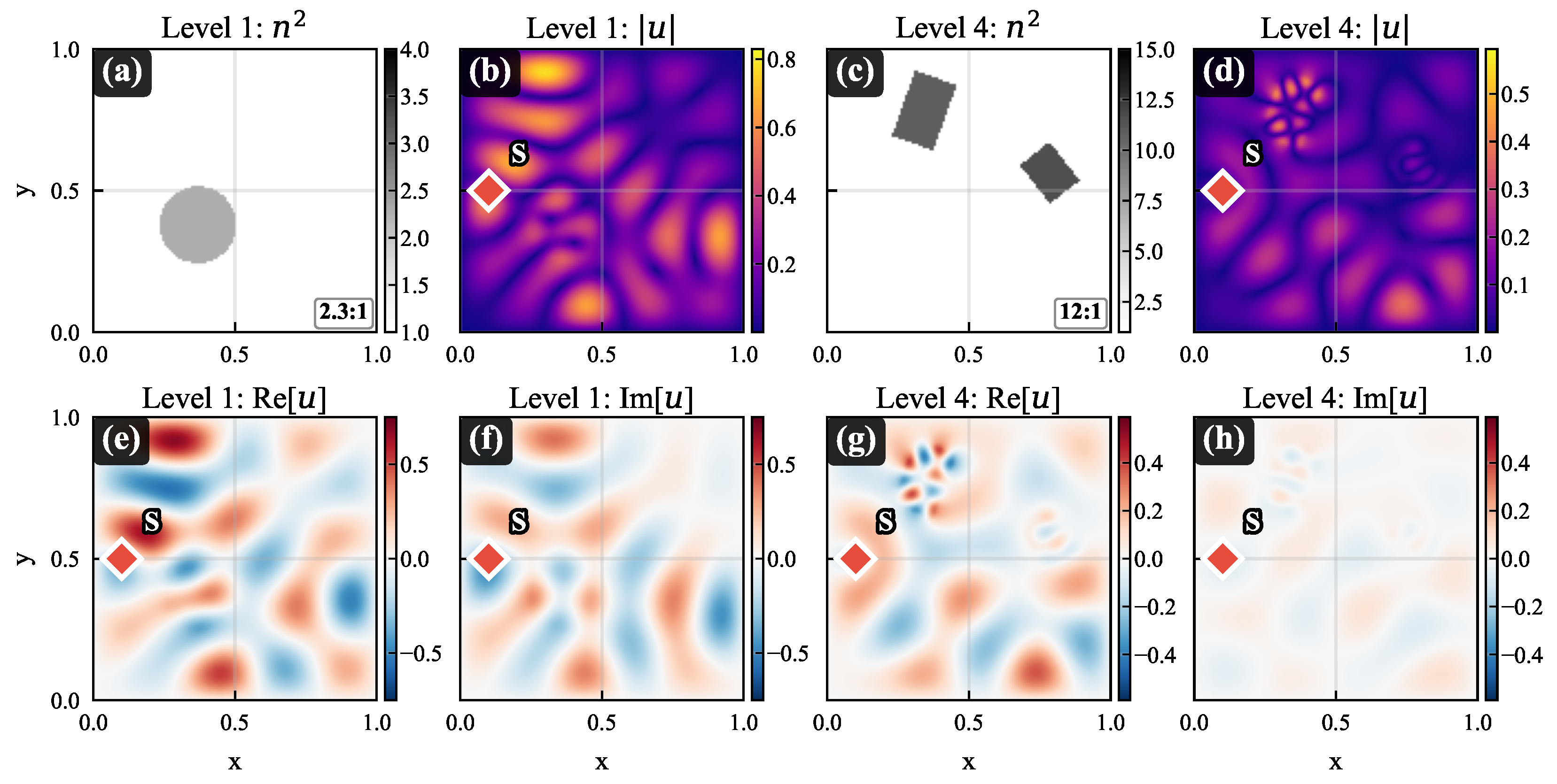
• Level 1 (Single): One circular scatterer with $n^2\in [1.5,3.0]$ on a unit background ($n_{\mathrm{bg}}^2=1$), giving a maximum contrast of 3:1.
• Level 2 (Multi): 2–5 non-overlapping scatterers with $n^2\in [1.5,3.0]$ on the unit background, maximum contrast 3:1.
• Level 3 (Random): Gaussian random field with Matérn-like power spectrum $P\left(k\right)\propto {(1+{(k\ell )}^2)}^{-2}$, correlation length $\ell =0.1$, clipped to $n^2\in [1.0,4.0]$.
• Level 4 (High Contrast): 1–4 high-contrast scatterers with $n^2\in [1.0,15.0]$ on the unit background, maximum contrast 15:1.

Of these four levels, only Level 3 is used for training and in-distribution evaluation, and only Level 4 is used for out-of-distribution testing (the precise train/validation/test split is detailed below); Levels 1–2 are not used during training and appear in Figure 2 purely for qualitative visualization of the complexity ladder. Figure 2 visualizes representative samples from Level 1 (simple) and Level 4 (high-contrast).

• Data splits, validation, and early stopping.

All models in this study are trained on Level 3 (random-blob) media only: a fixed pool of 800 training samples drawn from the Matérn-like Gaussian-random-field process with $n^2\in [1.0,4.0]$ (maximum contrast $\le 4:1$). Model selection and early stopping use a disjoint 100-sample Level 3 validation split (same generative process, different random seeds): training monitors the validation relative-$L^2$ loss, halts after 30 epochs without improvement (patience 30), and retains the lowest-validation-loss checkpoint; this same Level 3 split is the quantity reported as the in-distribution (InD) loss. Out-of-distribution generalization is then measured on a separate 100-sample Level 4 (high-contrast, $n^2\in [1.0,15.0]$, contrast up to $15:1$) test split that is never seen during training or checkpoint selection. This protocol underpins the central claim: because the entire high-contrast regime is held out of both training and model selection, the reported generalization gap measures genuine extrapolation across a complexity-and-contrast shift (random-blob, ≤$4:1\to$ discrete scatterers, ≤15:1) rather than within-distribution interpolation.

• Baselines.

We compare against three architectural families that span the design space of operator learning for this problem: the DeepONet branch–trunk family [2], a suite of FNO variants [1] spanning different parameter budgets, and the recent MscaleFNO architecture [6], which extends FNO with parallel frequency-scaled branches:

• DeepONet (parameter-matched): Vanilla branch–trunk operator; branch CNN (32, 64, 128, 256 channels), trunk MLP with $K_{\mathrm{F}}=64$ Fourier features, $4\times 256$ hidden, $p=128$ basis functions (1,046,318 params). Probes the structural family HNO sits inside, with neither our hybrid trunk nor our bounded factored branch.
• FNO-4m (baseline): Four modes, 4 layers (549,762 params).
• FNO-5m5L (parameter-matched): Five modes, 5 layers (1,053,634 params).
• FNO-4m7L: Four modes, 7 layers (955,458 params).
• FNO-6m4L: Six modes, 4 layers (1,205,122 params).
• MscaleFNO-N8 (parameter-matched): Eight frequency-scaled branches aggregated via learned weights (1,051,648 params).

All models are trained with identical hyperparameters, datasets, and random seeds for fair comparison. The parameter-matched models—DeepONet, FNO-5m5L, MscaleFNO-N8, and HNO—have ∼1.05 M parameters each (within ±0.6%). The main cross-architecture comparisons and the additional revision ablation series use 5 random seeds, while the remaining ablation and robustness studies use 3 seeds, reflecting the wall-clock budget of our single-GPU setup. Where 3-seed results are reported, we additionally indicate paired-t statistics so that the reader can assess whether the smaller sample is sufficient for the conclusion drawn.

• Metrics.

• Generalization Gap: $(L_{\mathrm{OOD}}-L_{\mathrm{InD}})/L_{\mathrm{InD}}\times 100\%$, where $L_{\mathrm{InD}}$ is the mean relative $L^2$ loss on the held-out Level 3 (random-blob) validation split—the in-distribution test set, drawn from the same generative process as training—and $L_{\mathrm{OOD}}$ is the loss on the Level 4 (high-contrast) test split. The gap is therefore a strict in-distribution-vs.-OOD comparison along a complexity-and-contrast shift (random-blob → discrete high-contrast scatterers, contrast $\le 4:1\to \le$15:1). The same metric is applied identically to all baselines.
• Inference Time: Wall-clock time per batch (averaged over 100 runs, after 50 warmup iterations).
• Statistical Tests: Paired (seed-by-seed) t-test, Cohen’s d effect size.

3. Results

3.1. Parameter-Matched Four-Way Comparison

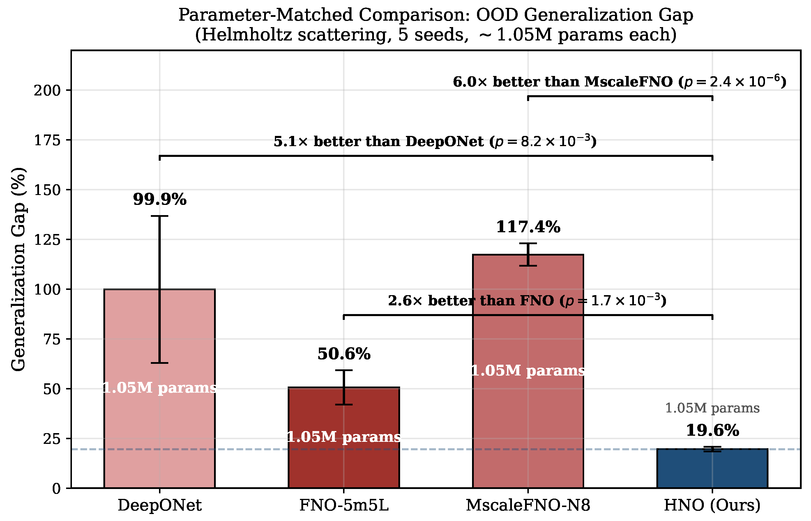
Table 1 presents results averaged over five random seeds. The parameter-matched quad (DeepONet, FNO-5m5L, MscaleFNO-N8, HNO) provides the fairest comparison: DeepONet probes the branch–trunk family that contains HNO (Section 2.3); FNO probes the fixed-spectral-basis approach; MscaleFNO probes the multi-scale capacity-scaling response to mode saturation; and HNO is the proposed architecture. Additional FNO configurations are reported for completeness. Figure 3 visualizes the generalization gap.

Three observations stand out before we turn to statistical tests. First, vanilla DeepONet does not fit the training distribution well (training loss ≈ 0.92, comparable to predicting zero), so its 99.9% OOD gap is driven by an underfitting trunk basis, not by overfitting; this directly isolates the value of HNO’s hybrid SIREN+learnable-Fourier trunk relative to the generic Fourier-feature trunk used by vanilla DeepONet. Second, FNO and MscaleFNO both reach low training loss (≈0.86) but generalize differently—50.6% versus 117.4% gap—confirming the mode-saturation/branch-overfitting reading of Section 1: adding parallel frequency-scaled branches worsens OOD generalization at matched capacity. Third, HNO has the lowest training loss (0.831) but the smallest gap (19.6%), with a monotone train < InD < OOD pattern. Our ablations (Section 3.4) attribute this small within-distribution overfit to the hybrid trunk and rank-32 modulator rather than to the bounded gate, which is accuracy-neutral; the gate acts as a stability guard while the wave-tailored trunk represents the Helmholtz field. We foreground the absolute relative $L^2$ errors alongside the gap: HNO attains 0.866 in-distribution and 1.036 out-of-distribution (Table 1). Every result below should therefore be read as a comparison of relative OOD robustness (the gap) rather than of absolute accuracy, which remains modest for every architecture in this extreme-contrast (15:1) regime. Section 3.6 discusses this absolute-accuracy ceiling and its practical consequences.

• Statistical Significance.

Paired t-tests across five identical seeds:

• HNO vs. DeepONet (matched params): Mean gap difference 80.3%, $t=4.87$, $p=8.2\times {10}^{-3}$ (large effect, despite DeepONet’s high cross-seed variance).
• HNO vs. FNO-5m5L (matched params): Mean gap difference 31.0%, $t=7.48$, $p=1.7\times {10}^{-3}$, Cohen’s $d=5.1$ (extremely large effect). (Throughout, Cohen’s d denotes the standardized mean difference computed with the pooled standard deviation of the two conditions ($d_s=31.0/6.13\approx 5.1$). The complementary paired effect size, $d_z=\left(\mathrm{mean}\mathrm{paired}\mathrm{difference}\right)/\left(\mathrm{SD}\mathrm{of}\mathrm{the}\mathrm{paired}\mathrm{differences}\right)=t/\sqrt{n}=7.48/\sqrt{5}\approx 3.3$ over the $n=5$ seeds, is itself a very large effect; we report the pooled d in the main text for comparability with common effect-size conventions. With $n=5$ seeds, the reported p-values reflect the low cross-seed variance of the matched comparisons rather than a large sample, and the effect-size estimates carry correspondingly wide confidence intervals; we therefore read them as evidence of a consistent, large architectural effect rather than as precise point values.)
• HNO vs. MscaleFNO-N8 (matched params): Mean gap difference 97.7%, $t=39.75$, $p=2.4\times {10}^{-6}$ (extremely large effect).
• HNO vs. MscaleFNO-N8-wide (4.2× MscaleFNO params): Mean gap difference 128.4%, $t=11.58$, $p=3.2\times {10}^{-4}$—HNO advantage persists and grows despite MscaleFNO’s capacity advantage.

Two observations strengthen the architectural interpretation. First, MscaleFNO’s OOD gap is monotonically worse with capacity (50.6% FNO → 117.4% narrow MscaleFNO → 148.0% wide MscaleFNO); adding parallel spectral branches does not merely fail to help—it actively hurts, and more capacity hurts more. Second, HNO’s standard deviation (1.1%) is 5–$22\times$ tighter than the FNO (8.6%), narrow-MscaleFNO (5.6%), and wide-MscaleFNO (24.8%) baselines, indicating that the coefficient-modulation architecture (the hybrid trunk and rank-32 modulator) yields not only better mean performance but also substantially more consistent behavior across seeds.

• Inference Speed.

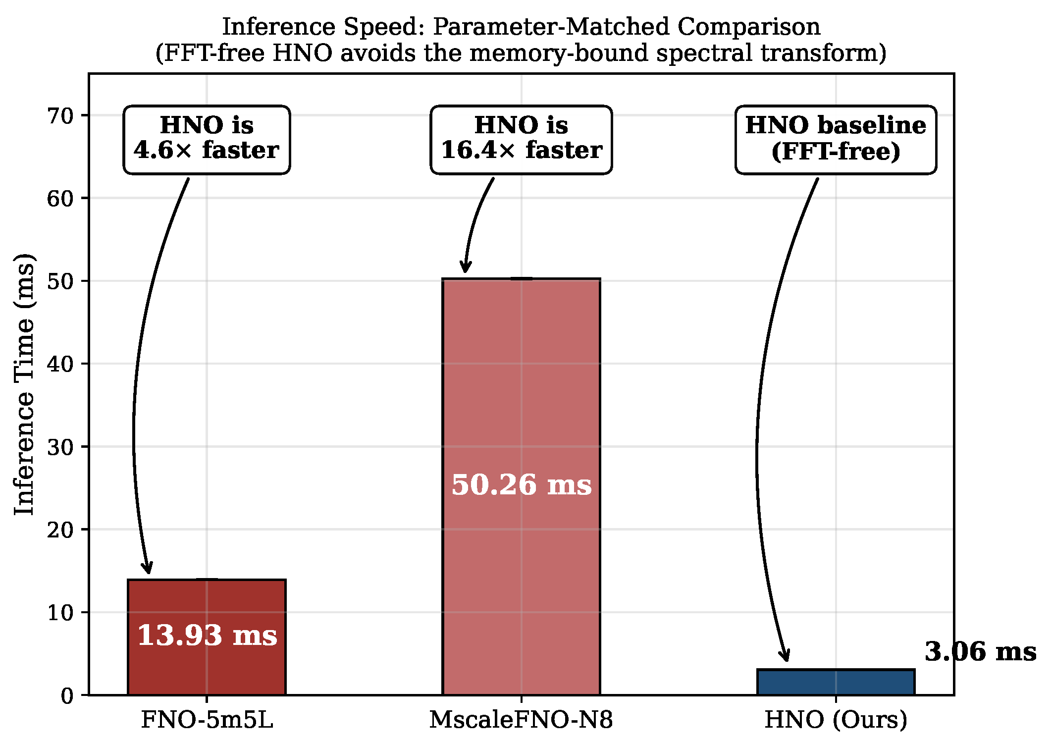
HNO achieves a 4.6× speedup over FNO-5m5L, a 16.4× speedup over MscaleFNO-N8, and a 29.6× speedup over MscaleFNO-N8-wide. This counterintuitive efficiency arises because

• FFT operations in FNO are memory-bound, not computing-bound, with poor cache locality.
• MscaleFNO amplifies this cost by running eight parallel FFT branches, each with its own spectral transform; widening each branch from 31 to 64 channels roughly doubles the per-branch FFT cost.
• HNO’s convolutions and linear layers achieve much higher GPU utilization on modern hardware (743.9 vs. 86.3 GFLOPS).
• HNO avoids the non-local memory access patterns inherent to butterfly FFT.

3.2. Wavelet Neural Operator Comparison

A natural question is how HNO compares against a learned non-Fourier fixed basis. We benchmark HNO against a Wavelet Neural Operator (WNO) that replaces the global FFT with a fixed Daubechies-4 (db4) discrete wavelet transform, at a comparable parameter budget under the identical PML/$k_0=20$ high-contrast protocol (Table 2). HNO attains the lowest absolute OOD error (1.036 vs. WNO 1.051) and the best in-distribution fit (0.864 vs. WNO 0.914). WNO’s smaller relative gap (15.0% vs. 19.9%) reflects its weaker in-distribution fit (InD $0.914$ vs. HNO’s $0.864$), which leaves less headroom for the gap to grow—a reminder that the gap must be read alongside the absolute OOD column rather than in isolation. Decisively, HNO is $14\times$ faster at inference (3.1 vs. 44.5 ms): WNO applies a discrete wavelet transform at every layer, whereas HNO is transform-free. HNO therefore matches or slightly beats WNO on accuracy while being an order of magnitude faster.

• Extreme contrast and multi-layer media.

To probe the boundary of out-of-distribution generalization beyond the $15:1$ Level 4 regime, we evaluate the Level 3-trained models on synthetically generated test sets at contrast ratios up to $50:1$ and on novel multi-layer (stratified-slab) media (

Table 3. Extreme-contrast (>15:1) and multi-layer OOD stress: relative $L_2$ of the Level 3-trained models (3 seeds, mean ± std). Test media are synthetically generated by the same FD-PML solver (Appendix A).

OOD Set	Contrast	HNO	FNO-5m5L
$20:1$ target	19.9:1	$1.046\pm 0.020$	$1.468\pm 0.169$
$30:1$ target	29.8:1	$1.064\pm 0.021$	$1.829\pm 0.305$
$50:1$ target	49.6:1	$1.049\pm 0.019$	$2.289\pm 0.484$
Multi-layer	29.8:1	$1.698\pm 0.048$	$12.267\pm 3.731$

). HNO’s relative $L^2$ stays near its ≈1.05 floor up to $50:1$, while FNO degrades from 1.47 to 2.29; on multi-layer media, FNO becomes catastrophic (12.27), whereas HNO remains bounded (1.70). We stress that an error near 1 is not accurate—it sits at the surrogate’s accuracy ceiling (Section 3.6)—so the finding is one of graceful degradation (HNO holds its floor while FNO diverges), not of accurate extreme-contrast prediction.

3.3. Frequency Robustness

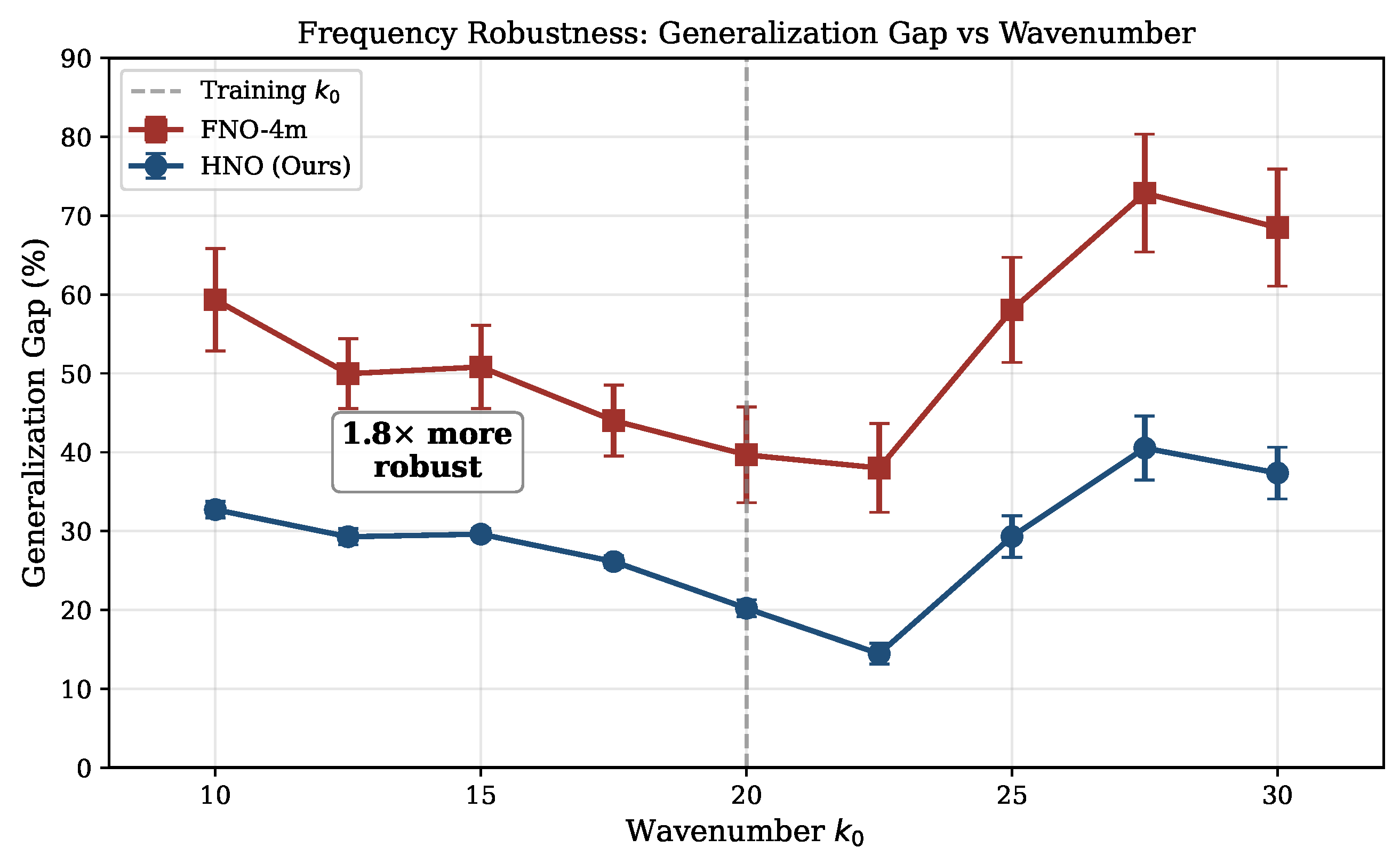
We train at $k_0=20$ and test across nine wavenumbers $k_0\in [10,30]$. Figure 4 shows that HNO maintains consistent performance while FNO degrades significantly at extreme frequencies; averaged over the swept wavenumbers, HNO attains a markedly lower mean OOD gap than FNO (29.9% vs. 55.2%) (

Table 4. Frequency robustness: Average OOD gap across $k_0$ values (excluding training $k_0=20$). Reported values are means over the eight swept wavenumbers (the nine-point sweep excluding the training $k_0=20$); the “Gap Variance” column is the spread across $k_0$, not a per-seed standard deviation (cf. the seed-wise ± convention used in Table 1). Bold marks the best (lowest) value in each column and the derived improvement row.

Model	Avg OOD Gap	Gap Variance
FNO-4m	55.2%	122.6
HNO	29.9%	53.8
Improvement	1.8×	56% lower

). (The FNO baseline used in this sweep is FNO-4m (550 K parameters, the configuration used as the FNO baseline in the original FNO paper for Helmholtz-like problems), not the parameter-matched FNO-5m5L (1.05 M) used in Section 3.1. The parameter-matched version of this sweep is reported below (

Table 5. Wavenumber-shift OOD gap (%) against the parameter-matched FNO-5m5L (3 seeds). Train $k_0=20$; the star marks the in-distribution wavenumber. Test sets at each $k_0$ are synthetically generated by the FD-PML solver (Appendix A).

${\mathit{k}}_{\mathbf{0}}$	FNO-5m5L	HNO	$\mathbf{\Delta }$
10.0	$+72.3$	$+32.7$	$+39.6$
12.5	$+59.3$	$+29.3$	$+30.0$
15.0	$+60.6$	$+29.6$	$+31.0$
17.5	$+52.1$	$+26.1$	$+26.0$
20.0 ⋆	$+50.8$	$+20.2$	$+30.6$
22.5	$+51.3$	$+14.4$	$+36.8$
25.0	$+69.0$	$+29.3$	$+39.7$
27.5	$+84.8$	$+40.5$	$+44.3$
30.0	$+81.9$	$+37.4$	$+44.6$

); the mode-saturation mechanism that drives FNO’s frequency sensitivity (Section 1) is a property of the fixed-spectral-basis architecture rather than of capacity, and the matched-capacity sweep confirms the qualitative pattern is preserved—indeed, the advantage widens.)

• Matched-capacity wavenumber sweep.

The sweep above uses the 550 K FNO-4m baseline (the configuration of the original FNO Helmholtz study); a reviewer asked for the comparison at the parameter-matched FNO-5m5L (1.05 M) used in the main evaluation. Repeating the sweep against FNO-5m5L (Table 5) widens HNO’s advantage rather than narrowing it: averaged over the swept wavenumbers ($k_0\ne 20$), HNO attains a 29.9% gap versus 66.4% for the matched FNO-5m5L—a $2.2\times$ robustness margin, larger than the $1.8\times$ margin obtained against FNO-4m, because the higher-capacity FNO overfits the training wavenumber more severely (consistent with the capacity–brittleness trend described in Section 3.1). At the training point $k_0=20$, both models reproduce the main comparison (FNO 50.8%, HNO 20.2%).

• Robustness to grid resolution and training set size.

HNO’s advantage is not an artifact of a single grid resolution or training set size. Across $64\times 64$, $128\times 128$, and $256\times 256$ grids, HNO attains a lower OOD loss than FNO at every resolution, and the margin widens with resolution; across training set sizes from 100 to 1000 samples, HNO retains the smaller generalization gap throughout, with the separation growing as data is added. The full sweeps are deferred to Appendix B (

Table A1. Grid resolution scaling: OOD loss at different spatial resolutions.

Resolution	HNO (OOD)	FNO (OOD)	Winner
$64\times 64$	1.078	1.278	HNO
$128\times 128$	1.036	1.306	HNO
$256\times 256$	1.018	1.366	HNO

and 

Table A2. Data size scaling: Generalization gap at different training set sizes.

Train Size	HNO Gap	FNO Gap	HNO Advantage
100	+10.5%	+19.9%	+9.4%
200	+13.4%	+16.0%	+2.6%
500	+16.6%	+39.1%	+22.5%
1000	+19.9%	+51.6%	+31.7%

) to keep the main comparison focused.

3.4. Architecture Ablation

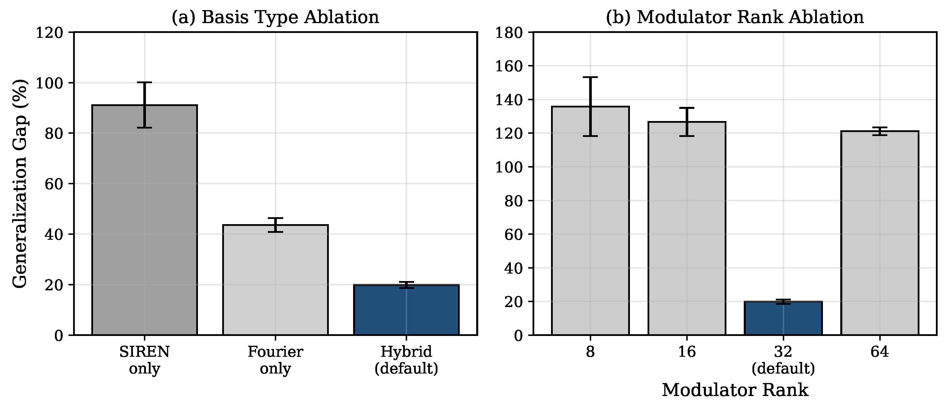
We ablate the three architectural choices of HNO—basis type, modulator rank, and encoder structure—in two complementary studies.

Table 6. Basis type and modulator rank ablation on the full HNO architecture (3 seeds). Each row modifies one component while keeping the rest of HNO fixed; the spatial-feature pathway in the modulator (Section 2.3) is preserved. Bold marks the best (lowest) generalization gap within each ablation group; italics mark the ablation-group header rows.

Configuration	Gen Gap	vs. Full HNO	Params
Basis Type Ablation
SIREN only	91.1 ± 9.0%	4.6× worse	768 K
Fourier only	43.6 ± 2.7%	2.2× worse	755 K
Hybrid (default)	19.9 ± 1.2%	–	1047 K
Modulator Rank Ablation
Rank 8	135.7 ± 17.5%	6.8× worse	748 K
Rank 16	126.7 ± 8.3%	6.4× worse	751 K
Rank 32 (default)	19.9 ± 1.2%	–	1047 K
Rank 64	121.1 ± 2.3%	6.1× worse	766 K

and

Table 7. Capacity-matched encoder ablation (3 seeds). The first three rows are matched at ∼1.05 M total parameters (∼915 K in the encoder); the fourth is a no-encoder control. All variants use the simplified backbone described in Section 3.4, so absolute gaps differ from Section 3.1; pairwise comparisons within the table are paired-seed. Bold marks the lowest generalization gap and its encoder row; bold in the footnote labels the statistically significant paired tests.

Encoder	Gen Gap	Params (Total)	Params (Encoder)
Linear (no activation)	207.3 ± 14.6%	1054 K	916 K
CNN (multi-scale conv)	64.6 ± 3.5%	1060 K	921 K
None (GAP + linear, control)	62.8 ± 16.8%	139 K	<1 K
MLP (flatten + bottleneck)	43.4 ± 10.1%	1054 K	916 K

Pairwise paired t-tests across 3 identical seeds: MLP vs. CNN: mean diff $-21.2\%$, $t=5.18$, $p=0.035$; CNN vs. Linear: $+142.7\%$, $t=-21.65$, $p=0.002$; CNN vs. no-encoder control: not significantly different ($\Delta =-1.8\%$).

report basis/rank ablations on the full HNO and a capacity-matched encoder ablation, respectively. Figure 5 visualizes the basis and rank sweeps.

• Capacity-matched encoder ablation.

A naive “with vs. without encoder” comparison conflates two confounds: the encoder’s structural prior (e.g., translation equivariance from convolutions) and its raw parameter capacity. To isolate these, we replace the encoder in HNO with three structurally distinct alternatives—CNN, MLP (flatten + nonlinear bottleneck), and Linear (flatten + low-rank linear projection, no activation)—all sized to ∼915 K encoder parameters (∼1.05 M total). A no-encoder control (global average pooling + scalar linear, 139 K total) is included as a reference floor. To attribute the effect to the encoder choice in isolation, all four variants share an identical backbone of HybridBasisNetwork + global-only modulator + coefficient network and omit the spatial-feature pathway used in the modulator of full HNO (Section 2.3). Absolute Gen Gap values in Table 7 are therefore higher than the 19.6% reported in Section 3.1; comparisons are between encoder variants within this simplified backbone.

• Key Findings.

• Hybrid basis is critical: Neither SIREN nor Fourier alone achieves good OOD generalization (Table 6).
• Rank 32 is optimal, with non-monotone behavior across ranks: The OOD gap drops by an order of magnitude between rank 16 (126.7%) and rank 32 (19.9%), then degrades again at rank 64 (121.1%). The interpretation that lower ranks (8, 16) bottleneck the modulator’s capacity to resolve enough independent directions in the medium-conditioning space, and that rank 64 hits an overfitting regime in which the hypernetwork captures medium-specific details that do not transfer to Level 4 contrast, is consistent with the gap pattern but is not the only possibility. The sharp ∼6× transition between rank 16 and rank 32, together with rank 64’s higher variance across reseeds in this and our earlier sweeps, also admits a training-stability reading: for example, the bounded tanh combiner output may saturate asymmetrically once the upstream LoRA dimension exceeds the rank-32 width tuned in the rest of the architecture. We do not distinguish the two readings here and treat rank 32 as a robust empirical operating point rather than as a fundamentally optimal capacity; the finer sweep at ranks 24, 32, 40, and 48 with multiple seeds, reported in Table 10, confirms a flat basin (18.6–21.0%) bracketed by the catastrophic ranks 16 and 64, supporting this training-stability reading.
• Nonlinear feature aggregation is essential, but the encoder’s spatial inductive bias is not: At matched capacity, the linear encoder collapses (+207% gap), confirming that nonlinearity in the encoder is required. However, neither CNN nor MLP dominates—in fact, MLP outperforms CNN by 21.2% at matched capacity ($p=0.035$), and the no-encoder control performs comparably to CNN ($\Delta =-1.8\%$, n.s.). Crucially, the ∼60% gaps in this table reflect its deliberately simplified backbone and must not be read as the effect of removing the spatial path: on the full backbone, the path-decomposition ablation (Table 9) shows that the global LoRA path alone already reaches a 20.4% gap, statistically indistinguishable from the full dual path (21.0%). The principal driver of the low gap is therefore not the spatial pathway but the hybrid trunk (Table 12: Hybrid 19.6% vs. Fourier 42.2% vs. SIREN 100.1%), together with an adequately sized rank-32 modulator, with the spatial path and encoder structure acting as comparatively minor robustness refinements.

• Additional ablations: gate-bound, dual-path, rank, and modulation form.

We report four further ablations requested in revision. These were run as an independent five-seed series; its default configuration ($|\Delta \varphi |\le 0.5$, rank 32, dual path, bounded gate) lands at a $21.0\%\pm 3.1$ gap, which is statistically consistent with—though slightly above—the $19.6\%\pm 1.1$ main result (Table 1), so we interpret only within-series comparisons. Three of the four return a robustness, not a necessity, verdict, which we state plainly. (i) Gate-bound (

Table 8. Gate-boundary sensitivity: OOD generalization gap as the coefficient-modulation bound $|\Delta \varphi |$ is varied (independent 5-seed series; see in-text baseline note).

Configuration	Params	In-Dist	OOD	Gen. Gap (%)
$|\Delta \varphi |\le 0.3$	1,047,440	0.867	1.050	$+21.2\pm 3.1$
$|\Delta \varphi |\le 0.5$ (ours)	1,047,440	0.867	1.050	$+21.0\pm 3.1$
$|\Delta \varphi |\le 0.7$	1,047,440	0.867	1.048	$+20.8\pm 3.1$
unbounded	1,047,440	0.867	1.031	$+18.9\pm 2.2$

): The OOD gap is insensitive to the multiplicative bound—$[-0.3,0.3]$, $[-0.5,0.5]$, $[-0.7,0.7]$, and unbounded all coincide within seed noise (unbounded $18.9\%$)—so $[-0.5,0.5]$ is a stable default and safety guard, not a tuned optimum. (ii) Dual path (

Table 9. Dual-path separation (global LoRA vs. spatial $1\times 1$-conv path): the spatial path is a refinement, not the principal driver, on the full backbone.

Configuration	Params	In-Dist	OOD	Gen. Gap (%)
global path only	1,047,440	0.866	1.043	$+20.4\pm 3.2$
spatial path only	1,047,440	0.867	1.050	$+21.0\pm 3.1$
both (ours)	1,047,440	0.867	1.050	$+21.0\pm 3.1$

): The global LoRA path alone ($20.4\%$) matches the full dual path ($21.0\%$), so the spatial path is a refinement, not the driver—correcting the simplified-backbone reading associated with Table 7. (iii) Modulation form (Table 11): Additive FiLM ($18.7\%$), attention ($20.8\%$), and dynamic routing ($17.2\%$) are comparable to the bounded multiplicative gate ($21.0\%$), so the OOD gain is insensitive to the gate form, and, as item (v) below shows, to the modulation’s presence altogether. (iv) Rank (

Table 10. Modulator-rank fine sweep around the chosen rank 32: ranks 24–48 form a flat basin.

Configuration	Params	In-Dist	OOD	Gen. Gap (%)
rank 24	1,042,304	0.867	1.031	$+18.9\pm 1.8$
rank 32 (ours)	1,047,440	0.867	1.050	$+21.0\pm 3.1$
rank 40	1,052,576	0.862	1.035	$+20.1\pm 2.1$
rank 48	1,057,712	0.865	1.026	$+18.6\pm 2.7$

): Ranks 24–48 form a flat basin ($18.6$–$21.0\%$) bracketed by the catastrophic ranks 16 and 64 of the coarse sweep (Table 12), so rank 32 is a robust operating point within a plateau rather than a sharp optimum, favoring the training-stability reading over a fine-tuned-capacity one. (v) Modulation presence (trunk/branch isolation) (

Table 11. Modulation mechanism and presence: the bounded-multiplicative coefficient gate vs. additive FiLM, attention, dynamic routing, and a no-modulation control ($\Delta \varphi \equiv 0$, i.e., a pure hybrid-trunk DeepONet at matched parameters). All variants—including removing the modulation outright—are comparable within seed noise (paired $t=-1.07$, $p=0.35$ for no-modulation vs. ours), so the modulation is accuracy-neutral on this benchmark and the hybrid trunk carries the OOD gain.

Configuration	Params	In-Dist	OOD	Gen. Gap (%)
bounded mult. (ours)	1,047,440	0.867	1.050	$+21.0\pm 3.1$
no modulation ($\Delta \varphi \equiv 0$)	1,047,440	0.866	1.043	$+20.4\pm 3.3$
additive FiLM	1,055,696	0.869	1.031	$+18.7\pm 1.5$
attention	1,047,440	0.866	1.046	$+20.8\pm 2.4$
dynamic routing	1,080,980	0.868	1.017	$+17.2\pm 1.4$

, “no modulation” row): Disabling the modulation outright (gate scale 0, so $\Delta \varphi \equiv 0$ and $\widehat{u}={\sum }_k{\alpha }_k\left(n^2\right){\varphi }_k^{\mathrm{hybrid}}\left(\mathit{x}\right)$—a pure hybrid-trunk DeepONet at the same $1,047,440$ parameters) leaves the OOD gap unchanged ($20.4\%$ vs. the full model’s $21.0\%$; paired $t=-1.07$, $p=0.35$, n.s.). This disentangles the two design choices that the matched-parameter DeepONet comparison alone confounds. Combined with the trunk swap (the vanilla MLP-trunk DeepONet of Table 1 at $99.9\%$ versus this hybrid-trunk DeepONet at $20.4\%$, matched capacity), it shows that essentially the entire $99.9\%\to 20\%$ OOD improvement is attributable to the hybrid wave-tailored trunk. The input-conditioned coefficient modulation is accuracy-neutral on this benchmark and is retained as a bounded, generic robustness mechanism rather than the accuracy driver. Finally, the core basis/rank/encoder ablation re-run at five seeds (

Table 12. Core architecture ablation (basis/rank/encoder) re-run at 5 seeds (addressing the request for ≥5 seeds); hybrid is the shared reference for all three axes. Bold marks the default (hybrid) reference row.

Configuration	Params	In-Dist	OOD	Gen. Gap (%)
SIREN only	767,905	0.860	1.721	$+100.1\pm 16.3$
Fourier only	755,265	0.900	1.280	$+42.2\pm 7.6$
Hybrid (default)	1,047,440	0.866	1.036	$+19.6\pm 1.1$
Rank 8	748,345	0.864	1.993	$+130.6\pm 17.9$
Rank 16	750,913	0.863	1.890	$+118.8\pm 10.7$
Rank 64	766,321	0.862	1.828	$+112.1\pm 21.6$
No encoder	139,345	0.921	1.831	$+98.8\pm 41.8$

, addressing the request for more seeds) confirms the load-bearing components: the hybrid trunk (Hybrid $19.6\%$ vs. Fourier $42.2\%$ vs. SIREN $100.1\%$), an adequately sized rank-32 modulator, and a nonlinear encoder.

3.5. Efficiency Analysis

Despite having ∼2.5× higher theoretical FLOPs than FNO (2.23 vs. 0.88 GFLOPs), HNO achieves 4.6× faster wall-clock inference than FNO-5m5L and 16.4× faster than MscaleFNO-N8 (Figure 6). (Speedup ratios in this subsection and in Figure 6 are computed from a dedicated FLOPs/speed benchmark run on the parameter-matched (∼1.05 M) configurations (HNO 3.06 ms, FNO 13.93 ms, MscaleFNO-N8 50.26 ms, MscaleFNO-N8-wide 90.55 ms). The “Inf. (ms)” column of Table 1 reports independently measured per-seed wall-clock averages (HNO 3.05 ms, FNO 13.98 ms, MscaleFNO-N8 50.48 ms); the two sources agree within run-to-run jitter (≲0.6%), well inside cross-seed variance, and yield nearly identical speedup ratios (e.g., MscaleFNO speedup $50.26/3.06=16.4\times$ vs. $50.48/3.05=16.6\times$).) This apparent paradox is explained as follows.

• Memory bandwidth: FFT operations are memory-bound with poor cache locality; MscaleFNO compounds this by running eight FFT branches in parallel.
• GPU utilization: HNO achieves 8.6× better GFLOPS utilization than FNO (743.9 vs. 86.3).
• Operation types: Convolutions and linear layers are highly optimized by cuDNN, whereas FFTs rely on batched cuFFT calls with less favorable memory layouts.

3.6. Comparison to Classical FD-PML Solver

The cross-architecture comparisons above establish HNO’s advantage over other neural operators but do not directly address a question of practical importance: When is a learned surrogate preferable to the classical solver that produced the training data? To answer this, we benchmark HNO inference against the same scipy-based five-point FD-PML solver used to generate our ground-truth dataset. Both methods are timed on the identical 100 Level 4 OOD samples. The FD-PML solver runs in single-process scipy.sparse with spsolve (SuperLU direct factorization); HNO runs on the GPU at the parameter-matched (∼1.05 M) configuration. CPU thread parallelism is restricted to one thread (MKL_NUM_THREADS=1) for deterministic timing.

• When the surrogate is preferable.

Table 13 quantifies the trade-off. The classical solver yields the reference ground-truth solution at 338 ms per query (75% of which is the LU factorization that must be repeated for every new medium $n^2$, since the system matrix changes with $n^2$). HNO returns a surrogate solution in $0.48$–$1.85$ ms, two-to-three orders of magnitude faster, at a cost of a relative $L^2$ error of ≈1.04 (≈104%) on Level 4 OOD samples (Table 1). Because this trade-off is conditional rather than universal, we make the operating regimes explicit:

• Regime 1—surrogate preferable (many-query, error-tolerant): Full-waveform inversion, parametric uncertainty quantification, design-space exploration, and real-time imaging issue ${10}^3$–${10}^6$ forward solves whose individual accuracy is absorbed by an outer loop. Here a 100×–700× wall-clock reduction translates directly into computing or response-time savings: a typical FWI loop with ${10}^4$ forward solves per inversion costs roughly an hour of CPU time with FD-PML versus ≈5 s with HNO. This is the regime the architecture targets.
• Regime 2—surrogate as warm-start only (accuracy-critical, many-query): When the same high-volume workload must also meet a tight accuracy tolerance, HNO is best used not as the final answer but as an initial guess polished by a small number of FD-PML (or Krylov) refinement steps near the solution—the surrogate sets the accuracy floor and refinement closes the residual. How few refinement steps suffice is an open question (Section 4.2).
• Regime 3—direct solver required (forward-once or high-accuracy): For single-shot or low-volume solves, PDE-constrained validation, and any application demanding solution-quality accuracy on extreme-contrast media, the ≈1 relative $L^2$ error is disqualifying, and the classical direct solver remains the correct choice; with a small query count, there is no amortization benefit.

Table 13. Wall-clock comparison on Level 4 OOD samples (100 problems, $128\times 128$ grid, $k_0=20$). FD-PML on Intel 12-core CPU, single-process scipy.sparse. HNO on NVIDIA RTX 3060 GPU. Per-sample times for HNO are reported both at batch size 1 (single query, e.g., real-time pipelines) and at batch size 32 (parametric sweeps). Speedups are wall-clock ratios; the accuracy column is taken from Table 1. Bold marks the HNO speedup factors and the recommended batched-inference configuration.

Method	Hardware	Per-Sample Wall-Clock	Speedup	Rel. ${\mathit{L}}^2$ Error	Use Case
FD-PML (scipy spsolve)	CPU, 1 thread	338.4 ms ± 6.8 ms	1× (reference)	≈0 (ground truth)	one-off solves, validation
assembly only	CPU, 1 thread	85.7 ms	–	–	–
LU solve only	CPU, 1 thread	251.8 ms	–	–	–
HNO (B = 1, single)	GPU (RTX 3060)	1.85 ms ± 0.10 ms	183×	1.04 (≈104%)	real-time inversion/imaging
HNO (B = 32, batch)	GPU (RTX 3060)	0.48 ms (per sample)	698×	1.04 (≈104%)	FWI, parametric UQ, design loops

Table 13. Wall-clock comparison on Level 4 OOD samples (100 problems, $128\times 128$ grid, $k_0=20$). FD-PML on Intel 12-core CPU, single-process scipy.sparse. HNO on NVIDIA RTX 3060 GPU. Per-sample times for HNO are reported both at batch size 1 (single query, e.g., real-time pipelines) and at batch size 32 (parametric sweeps). Speedups are wall-clock ratios; the accuracy column is taken from Table 1. Bold marks the HNO speedup factors and the recommended batched-inference configuration.

Method	Hardware	Per-Sample Wall-Clock	Speedup	Rel. ${\mathit{L}}^2$ Error	Use Case
FD-PML (scipy spsolve)	CPU, 1 thread	338.4 ms ± 6.8 ms	1× (reference)	≈0 (ground truth)	one-off solves, validation
assembly only	CPU, 1 thread	85.7 ms	–	–	–
LU solve only	CPU, 1 thread	251.8 ms	–	–	–
HNO (B = 1, single)	GPU (RTX 3060)	1.85 ms ± 0.10 ms	183×	1.04 (≈104%)	real-time inversion/imaging
HNO (B = 32, batch)	GPU (RTX 3060)	0.48 ms (per sample)	698×	1.04 (≈104%)	FWI, parametric UQ, design loops

Edge and embedded deployment (medical ultrasound, non-destructive evaluation) cuts across Regimes 1–2: the FFT-free, single-pass nature of HNO makes it portable to commodity GPUs and amenable to mobile-class accelerators, whereas the classical sparse solver depends on a system-level LAPACK/SuperLU stack.

• Caveats and stronger classical baselines.

The headline 183×/698× speedups in Table 13 are measured against the same single-process scipy.sparse.linalg.spsolve that produced the training data. Readers will fairly ask whether more sophisticated classical methods would close that gap. We therefore profile three additional baselines on the identical 100 OOD samples; the LU-solve wall-clock is reported in

Table 14. Extended classical-solver comparison (LU-solve wall-clock only; same 100 Level 4 OOD samples, $128\times 128$ grid, $k_0=20$, complex Helmholtz system, 3 repeats per sample). Assembly cost (≈86 ms per sample) is shared across all rows. The Converged? column reports whether the iterative solver reached a relative residual $\le {10}^{-6}$ within 200 iterations. The scipy.spsolve row (257.6 ms) was timed in a separate run on the same hardware as the 251.8 ms LU-solve number reported in Table 13; the ≈6 ms discrepancy is run-to-run jitter and is well within the standard deviation of either measurement. Bold marks the fastest classical solver (multi-threaded MKL PARDISO).

Classical Solver	Threads	Per-Sample Solve	vs. Scipy 1-Thread	Converged?	Notes
scipy.spsolve (SuperLU)	1	257.6 ms	1.00×	N/A (direct)	matches data-generation pipeline
pypardiso (Intel MKL PARDISO)	12	32.7 ms	7.88×	N/A (direct)	complex system embedded as $2\times 2$ real block
Classical AMG (pyamg)	1	700.3 ms	0.37×	0/100	diverges on indefinite Helmholtz operator
Shifted-Laplacian + AMG-FGMRES ($\beta =0.5$)	1	304.8 ms	0.85×	0/100	stagnates at residual $\approx 1.9$ within 200 iters

, with the assembly cost (≈86 ms per sample) shared across all variants.

Three observations follow. First, multi-threaded MKL PARDISO is $7.88\times$ faster than single-threaded spsolve, reducing the full FD-PML wall-clock per sample to ≈86 + 33 $\approx 119$ ms (assembly + solve). HNO’s speedup against this stronger classical baseline is therefore $119/1.85\approx 64\times$ at $B=1$ and $119/0.485\approx 245\times$ at $B=32$, rather than $183\times$/$698\times$. The smaller numbers are still a one-to-two-order-of-magnitude reduction; we report the headline ratio against the data-generation pipeline (single-threaded spsolve) for apples-to-apples comparison and the multi-threaded ratio here for engineering deployment fairness. Second, classical AMG (Ruge–Stüben on the real-block-form of A) does not converge on the indefinite Helmholtz operator at $k_0=20$ with $15:1$ contrast and is in fact $\approx 2.7\times$ slower than direct LU because of the wasted iterations. This is consistent with the well-known difficulty of geometric/algebraic multigrid for indefinite wave problems [23]. Third, a shifted-Laplacian preconditioner [23] (Erlangga–Oosterlee–Vuik 2006) with $\beta =0.5$ inside an AMG-preconditioned FGMRES does not reach the requested ${10}^{-6}$ tolerance within 200 iterations on our 100 samples; the residual stagnates around ≈1.9. A more carefully tuned shift schedule, deflation, or geometric multigrid V-cycle inside the preconditioner could close this gap (and is an active research area), but the result already shows that there is no single drop-in “classical Helmholtz solver” baseline—it is itself a research line.

• Amortized cost.

The per-query speedups above omit the one-time cost of building the surrogate, which a fair accounting must include: HNO must be trained, and its training data must itself be generated by the classical solver. Generating the 800-sample Level 3 training set costs $800\times 338\mathrm{ms}\approx 270$ s of FD-PML time (single-threaded spsolve, i.e., the data-generation pipeline), to which we add the one-time training wall-clock $T_{\mathrm{train}}\approx 34$ s for HNO (Appendix A). Against the single-threaded classical baseline, each HNO query saves ≈$338-0.5\approx 337$ ms at batch size 32, so the data-generation cost alone is recovered after ≈$270/0.337\approx 800$ queries—comparable to the dataset size itself—and the training-inclusive break-even $N^{\ast }=(270\mathrm{s}+T_{\mathrm{train}})/0.337\mathrm{s}\approx 900$ queries. Because the many-query workflows that motivate this work (FWI, parametric UQ) routinely issue ${10}^4$–${10}^6$ solves, the upfront cost is amortized by one-to-three orders of magnitude; for one-off or low-volume use (Regime 3 above), it is not amortized at all. A finer accuracy–cost characterization against higher-order finite-element (FEM) and geometric/algebraic multigrid solvers—reporting solution accuracy at matched wall-clock budgets rather than wall-clock at a fixed tolerance—is a natural extension and is left for future work.

The relative $L^2$ error of ≈1.04 on Level 4 OOD reflects an extreme contrast regime ($n^2$ up to 15:1), where even our best model is rough; on Level 3 in-distribution problems, the error drops to ≈0.87, and HNO’s advantage over FNO (Section 3.1) is in the relative OOD robustness, not in absolute accuracy.

3.7. Qualitative Comparison

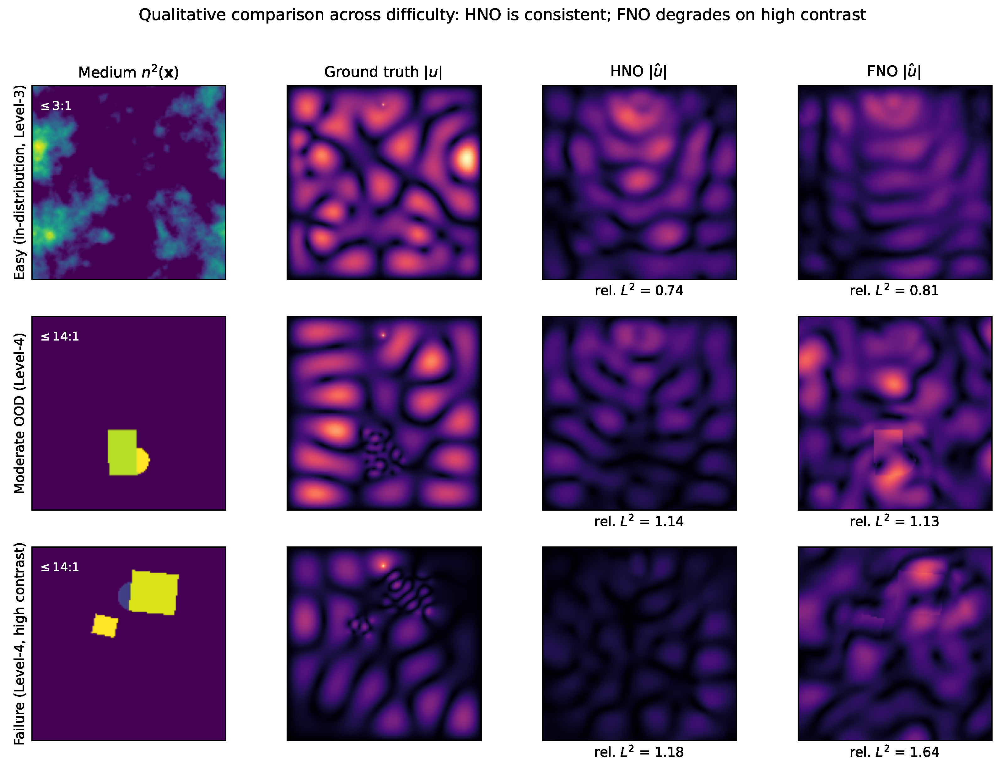
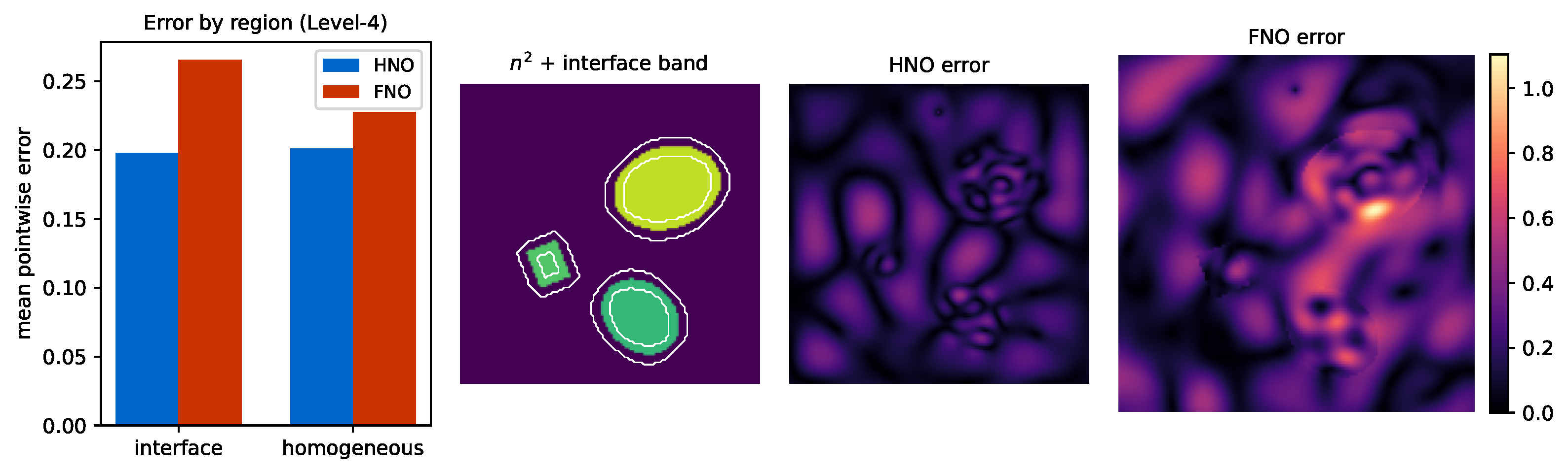
We compare FNO and HNO predictions qualitatively on Level 4 (high-contrast) OOD media. On the full 100-sample Level 4 test set, both models operate in an extreme-contrast regime (HNO mean relative $L^2\approx 1.04$ vs. FNO $\approx 1.30$), so the quantity of interest is not absolute accuracy but the spatial localization of error: whether FNO errors concentrate at material interfaces—where $n^2$ is discontinuous, consistent with mode saturation—while HNO stays more uniform through medium-conditioned coefficient modulation over the hybrid basis. We examine this first across the difficulty range (Figure 7) and then quantify it with an interface/homogeneous error decomposition (Figure 8); aggregate gap statistics are reported in Section 3.1.

• Easy, moderate, and failure cases.

Figure 7 compares HNO and FNO across the difficulty range: an easy in-distribution Level 3 medium, a moderate-contrast Level 4 medium, and a high-contrast Level 4 failure case. HNO’s relative $L^2$ stays bounded ($0.74/1.14/1.18$), while FNO degrades sharply on the high-contrast case ($0.81/1.13/1.64$); the two are comparable on the easy and moderate media. This makes concrete the aggregate statistics of Section 3.1: HNO is consistent across difficulty, whereas FNO is brittle on extreme contrast.

• Interface vs. homogeneous error decomposition.

We quantify the qualitative claim that FNO error concentrates at material interfaces while HNO is uniform. For each of the 100 Level 4 OOD samples, we split the domain into an interface band (a dilated neighborhood of large $|\nabla n^2|$) and the homogeneous interior, and average the pointwise error in each (Figure 8); the ratios below are computed from the full-precision regional means. FNO’s error is $1.17\times$ higher at interfaces than in homogeneous regions ($0.265$ vs. $0.227$), confirming interface-localized failure; HNO’s error is essentially uniform ($0.198$ vs. $0.201$, ratio $0.98\times$) and lower in both regions. The adaptive coefficient modulation thus removes the interface error concentration exhibited by the fixed Fourier basis.

4. Discussion

4.1. Scope: Darcy Flow as an Elliptic Counter-Example

We evaluate on the Darcy Flow benchmark [1], an elliptic PDE:

$$-\nabla ·\left(a\right(\mathit{x})\nabla u(\mathit{x}\left)\right)=f\left(\mathit{x}\right).$$

(10)

Figure 9 and

Table 15. Darcy Flow results (3 seeds; ± is the sample standard deviation). The baseline is the non-parameter-matched FNO-4m (550 K). FNO attains the lower gap on this elliptic benchmark, marking HNO’s wave-specialized scope; the large per-seed gap variance makes the ratio illustrative. Bold marks the lower (better) generalization gap, here attained by FNO.

Model	InD Loss	OOD Loss	Gen Gap
FNO-4m	0.094 ± 0.003	0.160 ± 0.014	70.6 ± 13.3%
HNO	0.090 ± 0.022	0.279 ± 0.028	229.8 ± 120.6%

summarize the outcome: on this elliptic benchmark, FNO attains the lower generalization gap, reversing the ordering observed on the Helmholtz problem.

• Why HNO Fails on Elliptic PDEs.

The architectural choices optimized for wave physics become liabilities for elliptic operators:

• SIREN periodicity: It is designed for oscillatory wave solutions ($u\sim \sin \left(k_{0}x\right)$), not smooth pressure fields.
• Hybrid basis: Fourier components are suited for global oscillations, not local diffusion.
• Bounded modulation: The $[-0.5,0.5]$ tanh constraint limits expressivity for monotonic solutions.

• Practical Guidance.

• Wave scattering, seismic, radar, ultrasound → Use HNO.
• Pressure diffusion, heat conduction, Darcy Flow → Use FNO.

The mismatch is expected from HNO’s design: its wave-tailored components (SIREN periodicity, hybrid Fourier basis, bounded modulation) suit oscillatory solutions, not the smooth, monotone fields of elliptic diffusion. We therefore treat the elliptic regime as outside HNO’s intended scope and recommend a general-purpose FNO there.

4.2. Further Limitations

Beyond the elliptic/hyperbolic scope boundary established above, we group the remaining limitations into seven categories: scope, wavenumber range, data and training cost, hardware, end-to-end inverse-problem validation, hyperparameter sensitivity, and geometric generality.

(a)

Scope: PDE class and dimensionality.

We validate HNO on the 2D Helmholtz equation with PML boundary conditions. Other wave-type PDEs of practical importance—Maxwell’s equations (electromagnetics), elastic wave equations (seismology), time-domain wave propagation, and 3D Helmholtz—are not evaluated. The architectural choices (SIREN periodicity and bounded coefficient modulation) are physically motivated for oscillatory solutions, and we expect the benefits to transfer, but direct evidence is out of scope here. The complementary elliptic case (Darcy Flow), where HNO is worse than FNO, is analyzed in Section 4.1 and is what bounds our claims to hyperbolic/wave operators rather than to operator learning in general. Two further coverage limits apply to the experimental setup itself: all results use a single fixed point-source location (${\mathit{x}}_s=(0.1,0.5)$; Appendix A) and the single Sommerfeld/PML boundary condition, so varied source configurations (multi-source, plane-wave, and distributed) and alternative boundary conditions are untested and left for future work—for reasons independent of the wavenumber-pollution argument of limitation (b). On the theoretical side, we establish no quantitative approximation-rate (n-width) bound for the medium-conditioned construction (Section 2.2); the out-of-distribution benefit is stated as a falsifiable empirical hypothesis and tested in Section 3.1 and Section 3.4, and a closed-form bound remains open.

(b)

Wavenumber range (low-to-moderate frequency only).

Training is performed at fixed $k_0=20$, and the frequency-robustness study (Section 3.3) sweeps test-time $k_0\in [10,30]$. With wavelength $\lambda =2\pi /k_0$ and domain side length $L=1$, this corresponds to $L/\lambda \approx 1.6$–$4.8$ wavelengths across the domain—the low-to-moderate frequency regime. Engineering Helmholtz applications often require substantially higher frequencies: seismic full-waveform inversion at the field scale operates at 30–100 wavelengths per profile [24], and ultrasound or microwave NDT can reach ∼${10}^2$–${10}^3$ wavelengths per device aperture. We therefore probe—rather than assume—the behavior just beyond the swept band with a limited high-wavenumber test at $k_0\in \{40,50,60\}$ (trained at $k_0=20$;

Table 16. High-wavenumber probe: OOD generalization gap (%) at test time $k_0\in \{40,50,60\}$ (trained at $k_0=20$; Level 4 high-contrast OOD, 3 seeds). The matched-parameter HNO advantage persists at every probed wavenumber; the $k_0\gtrsim 100$ regime is left untested (FD pollution error, Appendix A).

${\mathit{k}}_{\mathbf{0}}$ (ppw)	FNO-5m5L Gap %	HNO Gap %	$\mathbf{\Delta }$ (FNO−HNO)
40 (20)	$+101.0\pm 19.3$	$+42.7\pm 4.5$	$+58.4$
50 (16)	$+92.7\pm 18.0$	$+39.7\pm 3.7$	$+53.0$
60 (13)	$+114.9\pm 21.6$	$+47.0\pm 4.9$	$+67.9$
avg	$+102.9$	$+43.1$	$+59.8$

): the matched-parameter OOD advantage persists at every probed wavenumber, with HNO averaging a $43.1\%$ gap against FNO-5m5L’s $102.9\%$, even though both models’ absolute gaps rise well above their in-distribution values. We nonetheless make no high-frequency claim for the $k_0\gg 30$ regime as a whole—neither the 1.8× frequency robustness, nor quantitative OOD accuracy, nor the FD-PML speedup is demonstrated there. Two obstacles compound as $k_0$ grows, and each would require separate work. First, the second-order five-point FD ground truth itself incurs a pollution error scaling as $\mathcal{O}\left({\left(k_{0}h\right)}^2{k}_{0}L\right)$ [25] that would dominate for $k_0\gtrsim 100$ at our grid spacing (Appendix A), so even the training targets degrade unless a higher-order discretization or a finer grid is used. Second, FNO-style fixed-spectral methods need many more modes to resolve a high-frequency wavefield, so HNO would correspondingly need a larger basis budget K and likely a retuned SIREN frequency ${\omega }_0$. This subsumes solver fidelity more generally: higher-order discretizations or finite-element methods (FEMs) would shift absolute loss values, though—by the matched-baseline design—not the relative ordering across architectures. Extending HNO into the high-frequency regime is left for future work.

(c)

Data and training cost.

All main-text experiments use 800 Level 3 training samples, reflecting the single-GPU hardware budget. Our data-size ablation (Table A2, 100–1000 samples) shows HNO’s advantage over vanilla FNO is stable and actually grows with training set size within that range, but extrapolation beyond ${10}^3$ samples cannot be claimed from our data. We have tested MscaleFNO at 4.2× HNO’s parameter count and confirmed that the OOD gap worsens rather than narrows (Table 1), but large-scale training benchmarking at ${10}^4$–${10}^5$ samples against MscaleFNO remains for future work. The associated compute is itself a limitation: the main comparisons use five seeds and ablations use three seeds (Section 2.5), and the surrogate carries a one-time data-generation-plus-training cost (Section 3.6, “Amortized cost”) that is recovered only in the many-query regime. Per-model training time and peak GPU memory are reported in Appendix A for reproducibility.

(d)

Hardware.

Inference timings are measured on a single NVIDIA RTX 3060 (12 GB). The FFT memory-bottleneck argument (Section 3.5) may attenuate on newer GPUs with larger L2 caches or on TPUs with optimized spectral primitives. We expect the qualitative ordering to hold, but exact speedups are hardware-dependent.

(e)

End-to-end inverse-problem validation.

This paper validates HNO as a forward surrogate—we report relative $L^2$ error on the forward map $n^2\mapsto u$ and wall-clock speedups against FD-PML at the level of a single forward solve. We do not report end-to-end inverse-problem results, including full-waveform inversion with HNO as the inner-loop surrogate, parametric uncertainty quantification, or a closed-loop FWI-plus-FD-PML-refinement scheme (the warm-start Regime 2 of Section 3.6). Two questions become first-order in those settings and are not answered here: how the ≈1 relative $L^2$ error on Level 4 contrasts propagates through thousands of inverse-loop iterations (error accumulation, possible bias in the recovered medium), and how few FD-PML refinement steps suffice to reach inversion-quality accuracy when warm-started from HNO. Integrating HNO inside a full FWI loop and characterizing the surrogate-plus-refinement trade-off remain the most important future work for the applications that motivate this study (seismic FWI, parametric UQ, and real-time imaging in NDT and medical ultrasound).

(f)

Hyperparameter sensitivity and tuning cost.

The principal architectural hyperparameters—basis budget $K=64$, SIREN frequency ${\omega }_0=30$, modulator rank 32, and gate bound $[-0.5,0.5]$—were fixed once on the Level 3 validation split and then held constant across every experiment in this paper. The ablations of Section 3.4 indicate that the design is robust to the choices we did sweep: the OOD gap sits in a flat basin for ranks 24–48 (Table 10), is insensitive to the gate bound including the unbounded case (Table 8), and is essentially unchanged across bounded-multiplicative, additive-FiLM, attention, and dynamic-routing modulation forms (Table 11). We did not, however, jointly tune the basis budget K and the SIREN frequency ${\omega }_0$, nor did we retune any hyperparameter per wavenumber or per PDE class; a frequency-adaptive choice of K and ${\omega }_0$ is likely required to enter the high-$k_0$ regime of limitation (b), and a systematic or automated search over these settings is left to future work. The values reported here should therefore be read as robust defaults for low-to-moderate-frequency Helmholtz scattering, not as a globally optimized configuration.

(g)

Geometric generality (regular grids only).

All experiments use a regular $128\times 128$ Cartesian grid on the unit square with PML truncation. Both the SpatialFeatureEncoder (a multi-scale CNN) and the coordinate-evaluated hybrid trunk assume this structured, fixed-resolution layout, so the present architecture does not handle unstructured meshes, curved or re-entrant boundaries, or point-cloud discretizations. Operators built specifically for such settings—Geo-FNO and GINO (Section 1)—address geometry through explicit coordinate deformation or graph-kernel integration; combining HNO’s coefficient-modulation mechanism with a geometry-aware encoder of this kind is the natural route to irregular domains and is itself left for future work.

5. Conclusions

We introduced the Helmholtz Neural Operator (HNO), an FFT-free branch–trunk operator in the DeepONet family, combining a hybrid SIREN + learnable-Fourier trunk with a dual-path (rank-32 LoRA global + $1\times 1$-conv spatial) hypernetwork branch whose output is a bounded multiplicative gate on per-mode coefficients. On Helmholtz scattering benchmarks, we observe

• A 2.6× better OOD generalization than FNO at matched parameters (19.6% vs. 50.6% gap, $p=1.7\times {10}^{-3}$, $d=5.1$);
• A 5.1× better performance than vanilla DeepONet at matched parameters (19.6% vs. 99.9%, $p=8.2\times {10}^{-3}$)—an improvement a modulation-presence ablation (Section 3.4) attributes to the hybrid SIREN+Fourier trunk, with the coefficient modulation being accuracy-neutral;
• A 6.0× better performance than MscaleFNO at matched parameters (19.6% vs. 117.4%, $p=2.4\times {10}^{-6}$);
• A 7.6× better performance than MscaleFNO even at 4.2× more parameters (19.6% vs. 148.0%, $p=3.2\times {10}^{-4}$);
• Faster wall-clock inference via FFT-free design (HNO 3.06 ms): 4.6× vs. FNO-5m5L (13.93 ms, matched 1.05 M), 16.4× vs. MscaleFNO-N8 (50.26 ms, matched 1.05 M), and 29.6× vs. MscaleFNO-N8-wide (90.55 ms, 4.2× more parameters);
• A 1.8× better frequency robustness across wavenumber variations within the tested $k_0\in [10,30]$ band (Section 4.2);
• A 64×–245× faster performance than multi-threaded FD-PML (Intel MKL PARDISO on 12 cores), and a $183\times$–$698\times$ faster performance than the single-thread scipy.spsolve pipeline that produced our ground truth (Section 3.6), making HNO useful as a forward surrogate inside many-query workflows.

These speedups come with an explicit accuracy ceiling: on Level 4 OOD samples (15:1 contrast), the absolute relative $L^2$ error of HNO remains ≈1.04 (in-distribution ≈0.87), which dictates three deployment regimes (Section 3.6). HNO is the preferred forward map in many-query, error-tolerant workflows (inverse design, parametric UQ, real-time imaging); it should be used only as a warm start for a few FD-PML refinement steps when the same high-volume workload is accuracy-critical, and it is not a substitute for a classical direct solver in forward-once or high-accuracy settings. Because the one-time data-generation and training cost is recovered only after ∼${10}^3$ queries, the surrogate pays off in precisely the high-volume regimes that motivate it.

A notable empirical finding is that MscaleFNO, which scales spectral capacity through parallel frequency-scaled branches, degrades OOD generalization relative to vanilla FNO, and the degradation is monotonic in branch capacity—going from 50.6% (FNO, 1.05 M) to 117.4% (narrow MscaleFNO, 1.05 M) to 148.0% (wide MscaleFNO, 4.40 M). This rules out the hypothesis that matched-budget underperformance was an artifact of per-branch capacity starvation and points to the parallel-frequency-scaled decomposition itself as the source of OOD brittleness. The bottleneck for inhomogeneous wave scattering is not spectral expressivity but the wave-inappropriateness of a fixed Fourier basis; a hybrid SIREN+learnable-Fourier trunk addresses this directly, and our ablations (Section 3.4) locate the out-of-distribution gain in this trunk rather than in the medium-conditioned coefficient modulation, which is accuracy-neutral.

Importantly, HNO is specialized for hyperbolic/wave equations and underperforms on elliptic PDEs like Darcy Flow. This finding suggests that the future of neural operators may lie not in universal architectures but in physics-informed designs tailored to specific PDE classes.

• Engineering implications.

The efficiency and OOD-robustness gains reported here are expected to extend—subject to the high-frequency and closed-loop validation deferred in Section 4.2 (paragraphs (b) and (e))—to the settings that motivated this study: inverse-scattering and full-waveform inversion workflows in which a forward surrogate is invoked thousands of times, parametric uncertainty quantification over heterogeneous media, and real-time imaging pipelines in non-destructive evaluation and medical ultrasound. Because HNO does not rely on a global FFT, it avoids the spectral-primitive dependency of FNO-family surrogates and is amenable to deployment on commodity GPUs and edge devices.

• Future Work.

Promising directions include extending HNO to Maxwell’s equations (electromagnetics), elastic wave equations (seismology), and three-dimensional Helmholtz scattering, as well as tight coupling with classical PML-based finite-difference or finite-element preconditioners for inverse-scattering loops. Understanding which architectural features benefit which PDE classes could guide the design of problem-specific neural operators for applied science and engineering.

References

1. Li, Z.; Kovachki, N.; Azizzadenesheli, K.; Liu, B.; Bhattacharya, K.; Stuart, A.; Anandkumar, A. Fourier Neural Operator for Parametric Partial Differential Equations. arXiv 2021, arXiv:2010.08895. [Google Scholar] [CrossRef]
2. Lu, L.; Jin, P.; Pang, G.; Zhang, Z.; Karniadakis, G.E. Learning nonlinear operators via DeepONet based on the universal approximation theorem of operators. Nat. Mach. Intell. 2021, 3, 218–229. [Google Scholar] [CrossRef]
3. Kovachki, N.; Li, Z.; Liu, B.; Azizzadenesheli, K.; Bhattacharya, K.; Stuart, A.; Anandkumar, A. Neural Operator: Learning Maps Between Function Spaces with Applications to PDEs. J. Mach. Learn. Res. 2023, 24, 4061–4157. [Google Scholar] [CrossRef]
4. Pinkus, A. n-Widths in Approximation Theory; Springer Science & Business Media: Berlin/Heidelberg, Germany, 1985; Volume 7. [Google Scholar] [CrossRef]
5. DeVore, R.A.; Howard, R.; Micchelli, C.A. Optimal nonlinear approximation. Manuscripta Math. 1989, 63, 469–478. [Google Scholar] [CrossRef]
6. You, Z.; Xu, Z.; Cai, W. MscaleFNO: Multi-scale Fourier neural operator learning for oscillatory functions and wave scattering problems. J. Comput. Phys. 2026, 547, 114530. [Google Scholar] [CrossRef]
7. Liu, Z.; Cai, W.; Xu, Z.Q.J. Multi-scale deep neural network (MscaleDNN) for solving Poisson-Boltzmann equation in complex domains. Commun. Comput. Phys. 2020, 28, 1970–2001. [Google Scholar] [CrossRef]
8. Sitzmann, V.; Martel, J.; Bergman, A.; Lindell, D.; Wetzstein, G. Implicit neural representations with periodic activation functions. In Proceedings of the Advances in Neural Information Processing Systems, Virtual, 6–12 December 2020; Volume 33, pp. 7462–7473. [Google Scholar] [CrossRef]
9. Hu, E.J.; Shen, Y.; Wallis, P.; Allen-Zhu, Z.; Li, Y.; Wang, S.; Wang, L.; Chen, W. LoRA: Low-Rank Adaptation of Large Language Models. arXiv 2022, arXiv:2106.09685. [Google Scholar] [CrossRef]
10. Tripura, T.; Chakraborty, S. Wavelet Neural Operator for solving parametric partial differential equations in computational mechanics problems. Comput. Methods Appl. Mech. Eng. 2023, 404, 115783. [Google Scholar] [CrossRef]
11. Li, Z.; Huang, D.Z.; Liu, B.; Anandkumar, A. Fourier Neural Operator with learned deformations for PDEs on general geometries. J. Mach. Learn. Res. 2023, 24, 18593–18618. [Google Scholar] [CrossRef]
12. Li, Z.; Kovachki, N.; Choy, C.; Li, B.; Kossaifi, J.; Otta, S.; Nabian, M.A.; Stadler, M.; Hundt, C.; Azizzadenesheli, K.; et al. Geometry-Informed Neural Operator for Large-Scale 3D PDEs. arXiv 2023, arXiv:2309.00583. [Google Scholar] [CrossRef]
13. Balaji, A.; Teolis, T.; Mis, S.D.; Lara Benitez, J.A.; Wang, C.; de Hoop, M.V. Hybrid operator learning of wave scattering maps in high-contrast media. arXiv 2026, arXiv:2602.11197. [Google Scholar] [CrossRef]
14. Mildenhall, B.; Srinivasan, P.P.; Tancik, M.; Barron, J.T.; Ramamoorthi, R.; Ng, R. NeRF: Representing scenes as neural radiance fields for view synthesis. In Proceedings of the European Conference on Computer Vision; Springer: Berlin/Heidelberg, Germany, 2020; pp. 405–421. [Google Scholar] [CrossRef]
15. Tancik, M.; Srinivasan, P.; Mildenhall, B.; Fridovich-Keil, S.; Raghavan, N.; Singhal, U.; Ramamoorthi, R.; Barron, J.; Ng, R. Fourier features let networks learn high frequency functions in low dimensional domains. In Proceedings of the Advances in Neural Information Processing Systems, Virtual, 6–12 December 2020; Volume 33, pp. 7537–7547. [Google Scholar] [CrossRef]
16. Ha, D.; Dai, A.; Le, Q.V. Hypernetworks. arXiv 2017, arXiv:1609.09106. [Google Scholar] [CrossRef]
17. Perez, E.; Strub, F.; De Vries, H.; Dumoulin, V.; Courville, A. FiLM: Visual reasoning with a general conditioning layer. In Proceedings of the AAAI Conference on Artificial Intelligence, New Orleans, LA, USA, 2–7 February 2018; Volume 32, pp. 3942–3951. [Google Scholar] [CrossRef]
18. Daubechies, I. Ten Lectures on Wavelets; SIAM: Philadelphia, PA, USA, 1992. [Google Scholar] [CrossRef]
19. Candes, E.; Demanet, L.; Donoho, D.; Ying, L. Fast discrete curvelet transforms. Multiscale Model. Simul. 2006, 5, 861–899. [Google Scholar] [CrossRef]
20. Elad, M.; Aharon, M. Image denoising via sparse and redundant representations over learned dictionaries. IEEE Trans. Image Process. 2006, 15, 3736–3745. [Google Scholar] [CrossRef] [PubMed]
21. Gin, C.R.; Shea, D.E.; Brunton, S.L.; Kutz, J.N. DeepGreen: Deep learning of Green’s functions for nonlinear boundary value problems. Sci. Rep. 2021, 11, 21614. [Google Scholar] [CrossRef] [PubMed]
22. Greif, C.; Urban, K. Decay of the Kolmogorov N-width for wave problems. Appl. Math. Lett. 2019, 96, 216–222. [Google Scholar] [CrossRef]
23. Erlangga, Y.A.; Oosterlee, C.W.; Vuik, C. A novel multigrid based preconditioner for heterogeneous Helmholtz problems. SIAM J. Sci. Comput. 2006, 27, 1471–1492. [Google Scholar] [CrossRef]
24. Virieux, J.; Operto, S. An overview of full-waveform inversion in exploration geophysics. Geophysics 2009, 74, WCC1–WCC26. [Google Scholar] [CrossRef]
25. Babuška, I.M.; Sauter, S.A. Is the pollution effect of the FEM avoidable for the Helmholtz equation considering high wave numbers? SIAM J. Numer. Anal. 1997, 34, 2392–2423. [Google Scholar] [CrossRef]
26. Johnson, S.G. Notes on Perfectly Matched Layers (PMLs); Technical Report; Massachusetts Institute of Technology: Cambridge, MA, USA, 2008; MIT 18.369 Course Notes; Available online: http://math.mit.edu/~stevenj/18.369/pml.pdf (accessed on 15 February 2026).
Figure 1. Helmholtz Neural Operator (HNO) architecture. The SpatialFeatureEncoder extracts multi-scale features from the input medium n 2 ( x ) and exposes both a globally pooled vector z ( n 2 ) R 256 and a spatial feature tensor S ( n 2 ) R 128 × 32 × 32 . The dashed box delineates the EnhancedModulator, which combines a global path (rank-32 LoRA bottleneck on z ) and a spatial path (two 1 × 1 convolutions plus spatial pooling on S ) and routes the concatenated outputs through a 1 2 tanh combiner to produce the bounded multiplicative gate Δ ϕ ( n 2 ) [ 0.5 , 0.5 ] K . The HybridBasisNetwork combines SIREN and learnable Fourier bases evaluated at spatial coordinates x . The CoefficientNetwork takes z ( n 2 ) from the SpatialFeatureEncoder as input and predicts expansion coefficients α ( n 2 ) R 2 K for the final wave field reconstruction u ^ ( x ; n 2 ) = k α k ( n 2 ) ϕ k hybrid ( x ) ( 1 + Δ ϕ k ( n 2 ) ) . The architecture is FFT-free: spectral information is captured by the learnable Fourier feature block inside HybridBasisNetwork rather than by a global FFT.
Applsci 16 05997 g001
Figure 2. Dataset visualization. Top row: Input medium n 2 ( x ) and wave field magnitude | u ( x ) | . Bottom row: Real and imaginary components of the wave field. Level 1 (a,b,e,f) shows simple single-scatterer geometry; the displayed sample has a contrast 2.3 : 1 , while the dataset maximum is 3 : 1 . Level 4 (c,d,g,h) exhibits high-contrast multiple scatterers; the displayed sample has a contrast ≈12:1, while the dataset maximum is 15 : 1 . The numbers in brackets inside each medium panel report the contrast of the displayed sample; dataset-wide maxima are listed in the Section 2.5 above. A red diamond marked S indicates the point-source location. The increase in geometric and spectral complexity from Level 1 to Level 4 explains why fixed Fourier bases (FNO) struggle on Level 4.
Applsci 16 05997 g002
Figure 3. Parameter-matched comparison of OOD generalization gap across DeepONet, FNO, MscaleFNO, and HNO (∼1.05 M params each). Vanilla DeepONet (gray, leftmost) is the structural family HNO sits inside; its 99.9% gap with a generic Fourier-feature trunk and unconstrained branch quantifies the contribution of HNO’s hybrid trunk + bounded branch design at matched capacity. Adding parallel frequency-scaled branches (MscaleFNO) more than doubles the OOD gap relative to FNO, while HNO (blue, rightmost) achieves 2.6× better generalization than FNO ( p = 1.7 × 10 3 ), 5.1× better than DeepONet ( p = 8.2 × 10 3 ), and 6.0× better than MscaleFNO ( p = 2.4 × 10 6 ). A capacity-unmatched MscaleFNO with 4.2× more parameters further worsens to 148.0% (Table 1), confirming the observed collapse is architectural rather than capacity-related. The horizontal dashed line marks HNO’s generalization gap as a visual reference level.
Applsci 16 05997 g003
Figure 4. Frequency robustness: Generalization gap across wavenumber k 0 values. Training at k 0 = 20 (dashed line). HNO (blue) maintains lower and more consistent gaps compared to FNO-4m (red; the 550 K original-FNO baseline, not parameter-matched), demonstrating 1.8× better robustness with 56% lower variance; the parameter-matched FNO-5m5L sweep widens this margin to 2.2× (Table 5).
Applsci 16 05997 g004
Figure 5. Architecture ablation study (basis type and modulator rank). (a) Hybrid basis achieves 4.6× lower gap than SIREN-only and 2.2× lower than Fourier-only. (b) Modulator rank 32 is the critical sweet spot; both lower and higher ranks degrade substantially. The encoder ablation is reported separately in Table 7.
Applsci 16 05997 g005
Figure 6. Inference speed comparison (parameter-matched, ∼1.05 M params each). HNO achieves 4.6× faster inference than FNO (3.06 vs. 13.93 ms) and 16.4× faster than MscaleFNO (3.06 vs. 50.26 ms) due to its FFT-free design.
Applsci 16 05997 g006
Figure 7. Qualitative comparison across difficulty (seed-42 models). Rows: easy in-distribution Level 3, moderate Level 4, and high-contrast Level 4 failure. Columns: input medium n 2 , ground-truth | u | , HNO | u ^ | , FNO | u ^ | (relative L 2 annotated). HNO degrades gracefully ( 0.74 / 1.14 / 1.18 ), while FNO collapses on the high-contrast case ( 0.81 / 1.13 / 1.64 ). The medium panels (first column) use the viridis colormap (purple for low refractive index through green/yellow for high), and the wave-field magnitude panels (ground truth, HNO, FNO) use the magma colormap (dark for low magnitude through bright for high), each row on a shared scale.
Applsci 16 05997 g007
Figure 8. Interface vs. homogeneous error decomposition on Level 4 OOD (100 samples). Left: mean pointwise error by region (ratios from full-precision means)—FNO concentrates error at interfaces ( 1.17 × ) while HNO is uniform ( 0.98 × ) and lower in both. Right: a representative medium with the interface band (white contour) and the HNO/FNO error maps on a shared scale. In the medium panel (second from left), the viridis colormap shows the background in purple and the high-contrast scatterers in green/yellow, and the white contours delineate the interface band; the HNO and FNO error maps share the colorbar at right (magma colormap, dark for low error through bright for high).
Applsci 16 05997 g008
Figure 9. Darcy Flow (elliptic PDE), a deliberate out-of-domain test: FNO attains a lower gap than HNO (ratio ≈ 3.3×), marking the boundary of HNO’s wave-specialized design. The Darcy baseline is the non-parameter-matched FNO-4m (550 K), and the per-seed gap variance is large, so the ratio is illustrative rather than precise.
Applsci 16 05997 g009