Physics-Informed Residual Convolutional Network Model for Depth-Averaged Landslide Dynamics

Abstract

Rapid landslide motions control impact area, flow velocity, deposition pattern, and, in extreme cases, are a river-blocking hazard; therefore, reliable dynamic simulations are of direct importance to engineering–geological hazard assessments. Depth-averaged models provide an efficient framework for simulating large-scale mass movements, but conventional physics-informed neural networks (PINNs) remain challenged with regard to nonlinear flows, which can limit their applicability in landslide analysis. To address these limitations, this study develops a physics-informed residual convolutional network model (PI-RCN) for depth-averaged landslide dynamics. The proposed framework combines sequential residual learning with depth-wise separable convolutions (DSCs) and incorporates physics-based residuals, mass conservation, and hard constraints to preserve physical consistency during time marching. The model is evaluated using a 1+1D frictionless dam-break benchmark, a Hong Kong landslide, and the Yigong rock avalanche. Results show that PI-RCN accurately reproduces the benchmark flow evolution with substantially fewer trainable parameters than a baseline fully connected PINN. In the Hong Kong case, the model demonstrates improved convergence stability and optimization efficiency. In the Yigong case, PI-RCN reproduces the main spatiotemporal evolution and multi-stage velocity variation of a long-runout rock avalanche. These results suggest that PI-RCN provides a useful physics-informed framework for efficient and consistent landslide dynamic simulation.

1. Introduction

In mountainous regions, floods, glacial hazards, and landslides pose increasingly serious threats to human lives and infrastructure. The dataset indicates that 4862 distinct landslide events caused a total of 55,997 fatalities between January 2004 and December 2016 [1]. To mitigate these risks, it is essential to understand not only where such hazards may occur, but also how they initiate and evolve in space and time. This need has motivated the development of dynamic risk analysis frameworks capable of simulating the initiation, propagation, and runout of hazardous mass movements [2]. Within this context, hazard zoning has become a fundamental component of urban and regional planning [3]. Effective hazard zoning relies on dynamic analysis to solve the governing equations of motion, enabling quantitative predictions of key physical indicators such as runout distance, flow velocity, and impact extent. These parameters are critical for assessing hazard intensity and delineating hazard-prone areas, making dynamic numerical modeling an important tool in hazard assessment [4].

To meet the computational demands of such dynamic analyses, depth-averaged models are derived by averaging the three-dimensional governing equations over the vertical direction, resulting in a system of two-dimensional equations that describe horizontal motion [5]. This reduction in dimensionality significantly decreases computational cost while retaining the essential dynamics of large-scale flows. These models are widely adopted in landslide simulations [6,7,8].

Depth-averaged models rely on several key assumptions, including incompressible flow with constant density ρ [5], negligible vertical variations [9], and dominant dynamics in the horizontal plane. Representative examples include the shallow water equations, the Savage–Hutter model [5], and Boussinesq-type models [10], which have been extensively applied to simulate floods, landslides, and debris flows.

Depth-averaged models have advanced toward multiphase formulations. Notably, Pudasaini [11] introduced a generalized two-phase dynamic model, while Pudasaini and Mergili [12] developed a multiphase landslide dynamics model to describe the motion patterns of distinct phases. The primary strengths of depth-averaged models reside in their computational efficiency and simplicity, rendering them ideal for numerical simulations. Despite their simplifications, these models can capture the essential dynamical characteristics of geophysical flows.

For the governing equations of geophysical mass flows, numerical methods constitute an important component of the solution process. Two fundamental descriptions are commonly adopted: the Lagrangian and Eulerian frameworks. The Lagrangian description follows the trajectories of individual particles and requires explicit computation of the forces acting on each particle, making it particularly suitable for problems involving a limited number of discrete elements [13,14]. Representative Lagrangian-based software includes LS-Rapid [2], Landslide Analyst (LA) [15], Debris Flow Analyst (DA) [16], and Rapid Mass Movement Simulation (RAMMS, https://ramms.ch/ (accessed on 18 May 2026)) [17].

In contrast, the Eulerian description observes the evolution of flow variables at fixed grids, which is more appropriate for continuum-scale simulations [18,19]. Owing to its efficiency and robustness in handling large deformations and long runout processes, the Eulerian framework has been widely adopted in modeling rock avalanches and debris flows [20,21]. Key examples of Eulerian-based software include r.avaflow (https://www.avaflow.org/ (accessed on 18 May 2026)) [22], Titan2D (https://github.com/titan2d/titan2d (accessed on 18 May 2026)) [23], and Massflow (http://www.massflow-software.com/en/ (accessed on 18 May 2026)) [24].

Despite the various simplifications incorporated into hydrological dynamic models, analytical solutions are rarely available for realistic flow conditions. Consequently, numerical discretization schemes are required to obtain approximate solutions. Traditional approaches primarily include the finite difference (FD) method [25] and the finite volume method (FV) [26]. In hydrological simulations, FD and FV methods discretize the governing equations into systems of algebraic equations that can be solved using matrix-based techniques. To ensure numerical stability and accuracy, various linearization and discretization strategies have been developed, such as the non-oscillatory central (NOC) differencing scheme [27] and the MacCormack scheme [24].

In addition, flux-splitting techniques are widely employed to handle strong nonlinearities and discontinuities by decomposing fluxes into positive and negative components. Prominent examples include the Steger–Warming flux-splitting scheme [28], Van Leer flux splitting [29], and Liou–Steffen flux splitting [30]. While these schemes have proven effective, their performance is often highly sensitive to algorithm selection, parameter tuning, and mesh resolution, which can pose significant challenges for practical and large-scale applications. Alongside grid-based methods, advances in computing technology have facilitated the development of meshless techniques, such as smoothed particle hydrodynamics (SPH) [31,32]. However, SPH simulations remain dependent on particle number and spatial distribution, which can substantially influence solution accuracy.

Physics-informed neural networks (PINNs) have emerged as a promising alternative for solving partial differential equations (PDEs) by embedding physical laws directly into the neural network training process [33]. PINNs have been widely applied across multiple geotechnical-related fields, including geotechnical methods [34], landslide simulation [35], and earthquake engineering [36]. By avoiding explicit mesh generation and traditional discretization, PINNs offer an appealing framework. Nevertheless, PINNs suffer from several limitations that restrict their robustness and scalability. In particular, when applied to stiff, multi-scale, or highly nonlinear systems, PINNs often exhibit training instability and slow convergence due to ill-conditioned loss landscapes and severe gradient imbalance between PDE residuals and boundary or initial condition constraints [37,38]. Moreover, the inherent spectral bias of neural networks limits their ability to accurately resolve high-frequency components, sharp gradients, and discontinuities, which are common in advection-dominated flows, shock waves, and granular or landslide dynamics [39]. These difficulties are further exacerbated by strong sensitivity to hyperparameter choices and the absence of rigorous convergence guarantees for complex nonlinear PDEs, often resulting in suboptimal solutions or prohibitively high computational costs.

PINNs remain challenged by slow convergence, training instability, and limited capabilities in resolving sharp gradients and strongly nonlinear flow features in depth-averaged geophysical mass movements. These limitations restrict their practical applicability to large-scale and highly transient landslide simulations. This study proposes a physics-informed residual convolutional network (PI-RCN) for depth-averaged landslide dynamics, in which residual learning is integrated with depth-wise separable convolutions (DSCs) to improve gradient propagation, enhance training stability, and reduce computational complexity.

The main contributions of this work include three aspects. First, we develop a physics-informed residual convolutional framework for sequential prediction of depth-averaged landslide motion. Second, the combination of residual learning and DSC improves optimization efficiency while preserving the capability to represent strongly nonlinear spatiotemporal evolution. Third, through benchmark and real-case analyses, we demonstrate that the proposed framework has the potential to support engineering–geological assessment. These outputs of the model are directly related to hazard zoning and risk assessment. This study provides a useful tool for landslide hazard analysis using a convolutional network model.

2. Materials and Methods

Based on the dynamic process, key landslide indicators, such as runout distance, affected area, and deposition pattern, can be obtained to support landslide mobility analysis and hazard assessment. Unlike conventional numerical algorithms such as the finite difference method, which are usually designed for specific governing equations and physical models, this study develops a general physics-informed framework based on neural network design. The PI-RCN embeds the conservation constraints of depth-averaged landslide dynamics into a learnable spatiotemporal structure to predict the temporal evolution of flow depth and depth-averaged velocity.

2.1. Framework

(1)

Time-Marching Strategy

In PI-RCN, the solution is advanced sequentially in time through a time-marching framework. Starting from the initial flow state, the network predicts the flow variables at the next time level, and the predicted state is then used as the input for the subsequent step. The flow field is propagated step by step as

$${\mathbf{U}}^0\stackrel{\mathsf{\Delta }t}{\to }{\mathbf{U}}^1\stackrel{\mathsf{\Delta }t}{\to }\cdots \stackrel{\mathsf{\Delta }t}{\to }{\mathbf{U}}^n\stackrel{\mathsf{\Delta }t}{\to }{\mathbf{U}}^{n+1}.$$

(1)

where ${\mathbf{U}}^n$ denotes the flow state at time level $n$. The initial state is constructed from the initial flow thickness together with zero initial momentum, and two historical states are maintained during the simulation to support multi-step temporal discretization. Specifically, ${\mathbf{U}}^n$ is used as the current input state, while ${\mathbf{U}}^{n-1}$ is retained once available for higher-order time integration.

To improve temporal stability and efficiency, an adaptive time increment is employed. At each marching step, the time step size is determined according to a CFL-type criterion based on the local flow velocity and gravity wave speed

$$\mathsf{\Delta }t=\mathrm{c}\mathrm{l}\mathrm{i}\mathrm{p}\left({\displaystyle \frac{CFL\cdot \min \left(\mathsf{\Delta }x,\mathsf{\Delta }y\right)}{\max \left(\sqrt{u^2+v^2}+\sqrt{gh}\right)+\epsilon }},\mathsf{\Delta }{t}_{min},\mathsf{\Delta }{t}_{max}\right)$$

(2)

This strategy improves numerical robustness while avoiding unnecessarily small-time steps.

The number of optimization steps is set to be larger in the initial stage and reduced in later stages, reflecting the fact that the early evolution requires stronger correction from the randomly initialized model, whereas later stages can benefit from parameter inheritance from the previous step. Therefore, the temporal training is not restarted independently at each step; instead, the network weights obtained at the previous time level are directly reused and further updated at the current step. This parameter continuation mechanism serves as a physics-informed fine-tuning process across adjacent time levels and exploits the temporal similarity of consecutive landslide states.

A mixed first- or second-order backward differentiation strategy is adopted for temporal discretization. For the first marching step, a first-order backward difference formula (BDF₁) is used because only the initial state is available. After the second state has been obtained, the method switches to a second-order backward difference formula (BDF₂), which incorporates both ${\mathbf{U}}^n$ and ${\mathbf{U}}^{n-1}$ to construct the temporal residual at ${\mathbf{U}}^{n+1}$. In the code implementation, the BDF₁ residual is used only at the initial step, whereas all subsequent steps are optimized using the BDF₂ residual. This design provides a stable start-up procedure and improves temporal accuracy during the later propagation stage.

After the optimization converges, the trained network is applied to the current state ${\mathbf{U}}^n$ to predict ${\mathbf{U}}^{n+1}$. Through this sequential prediction–update procedure, PI-RCN simulates landslide motion while preserving temporal consistency and computational efficiency.

(2)

Residual Block Design

PI-RCN is formulated to learn the temporal increment of the state variable rather than directly predicting the full flow state at the next time level. Specifically, for the flow state ${\mathbf{U}}^n$ at time level $n$, the neural network is designed to approximate the residual evolution as

$$\begin{array}{c}{\mathcal{N}}_{\theta }\left({\mathbf{U}}^n\right)={\mathbf{U}}^{n+1}-{\mathbf{U}}^n\end{array}$$

(3)

where ${\mathcal{N}}_{\theta }\left(\cdot \right)$ denotes the trainable nonlinear mapping parameterized by $\theta$.

This residual formulation allows the network to concentrate on learning the incremental physical evolution between two adjacent time levels. Since consecutive landslide states are usually strongly correlated in time, the temporal increment is generally smoother and easier to approximate than the full solution field. As a result, the optimization process becomes more stable and efficient, particularly for strongly nonlinear transient dynamics.

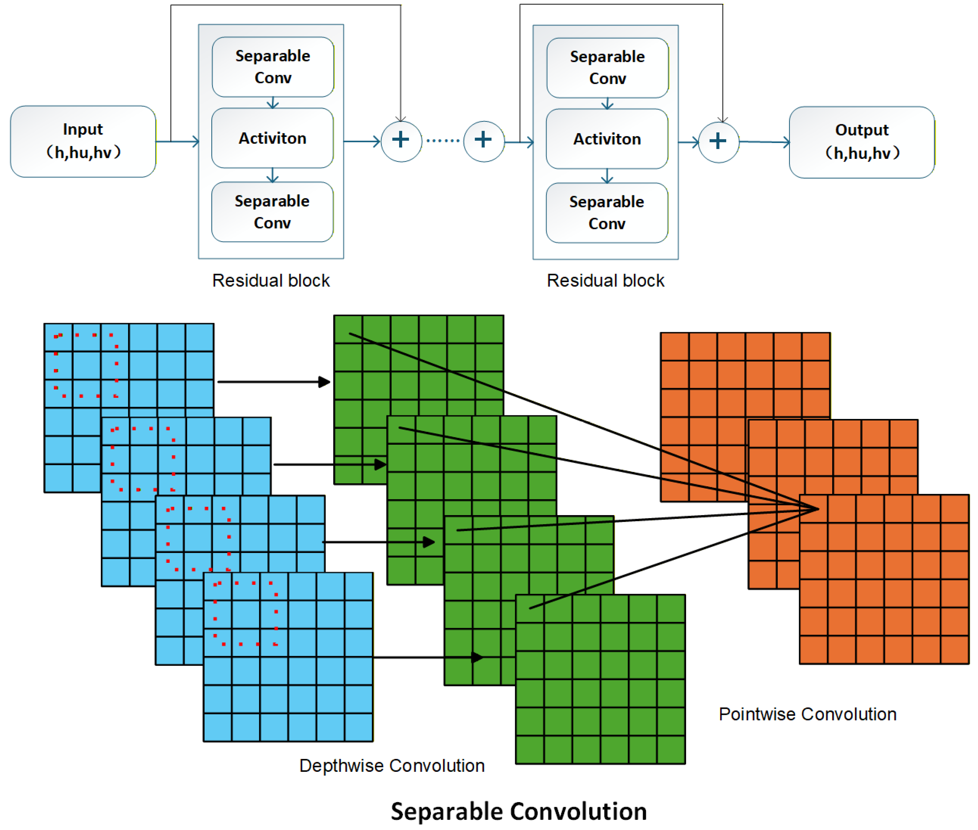
Building upon the residual learning strategy, a DSC-Residual Block is constructed, as illustrated in Figure 1. Each block contains two successive DSC layers, each followed by nonlinear activation, together with an identity shortcut connection. The transformed features are added to the input feature map to form the block output. This design preserves input information, improves gradient propagation during backpropagation, and enhances training stability in deep architectures. By stacking multiple DSC-Residual Blocks, the network can progressively capture the complex nonlinear spatiotemporal features of landslide motion.

In addition, the residual formulation is consistent with the sequential time-marching strategy adopted in PI-RCN. At each time level, the model receives the current state as input and predicts only the update required to advance the solution to the next time level. This design reduces the learning burden of each forward pass and makes the model particularly suitable for simulation. The residual block serves both as a structural mechanism for stabilizing deep-network training and as a physically motivated operator for learning the incremental evolution of landslide dynamics.

(3)

Depth-wise separable convolutions

To reduce computational cost and improve inference efficiency, the standard convolutional layers in PI-RCN are replaced with a DSC. A conventional convolution simultaneously performs spatial filtering and cross-channel feature mixing within a single operation. In contrast, a DSC decomposes this process into two successive steps: a depth-wise convolution, which applies an independent spatial filter to each input channel, and a pointwise convolution with a 1 × 1 kernel, which linearly combines the resulting channel-wise features to produce the output channels. This decomposition preserves the capability of spatial feature extraction while substantially reducing the number of trainable parameters and floating-point operations (FLOPs). For an input feature map H of spatial size $D_f \times D_f$, let the convolution kernel size be $k \times k$, and let the numbers of input and output channels be $C_{in}$ and $C_{out}$, respectively. The resulting output feature map G has a spatial size $D_g\times D_g$. These expressions are summarized in

Table 1. Comparison of parameter counts and FLOPs between the standard convolution and DSC.

	Parameters	FLOPs
Convolution	$k^2{C}_{in}{C}_{out}$	$k^2{C}_{in}{C}_{out}{D}_g^2$
Separable convolution	$k^2{C}_{in}+C_{in}{C}_{out}$	$k^2{C_{in}D}_g^2+D_g^2{C}_{in}{C}_{out}$

. Under the same output feature map size, the parameter and FLOP ratios of DSCs relative to the standard convolution ($R_P \mathrm{a}\mathrm{n}\mathrm{d} R_{FLOPS}$) have the same form. The ratios are:

$$R_P=R_{FLOPS}={\displaystyle \frac{1}{C_{out}}}+{\displaystyle \frac{1}{k^2}}$$

(4)

The ratios provide quantitative measures of how much computational cost can be saved by replacing a standard convolution with a depth-wise separable convolution. A smaller value indicates a stronger reduction in model complexity and computational cost. Compared with standard convolution, DSC becomes increasingly efficient as $C_{out}$ and $k$ increase.

As a representative example, when $k=3$, $C_{in}=32$, and $C_{out}=64$, the number of trainable parameters is reduced from 18,432 for the standard convolution to 2336 for DSC, corresponding to an 87.3% reduction. This substantial decrease in model complexity highlights the efficiency benefit of the separable design, which is particularly advantageous for large-scale spatiotemporal modeling tasks such as landslide dynamics, where repeated feature extraction is required throughout sequential time marching. In PI-RCN, this convolution strategy enables the network to maintain strong nonlinear representation capabilities while improving optimization efficiency and reducing overall computational burden.

By incorporating DSCs into the residual blocks, PI-RCN achieves a compact architecture that is suited to physics-informed simulations of nonlinear depth-averaged flows. The reduced computational complexity allows more efficient training and inference, while the residual structure preserves stable gradient propagation. The overall network architecture built upon this design is presented in Figure 2.

2.2. Hard Constraints

Two hard constraints are incorporated into PI-RCN: non-negativity of flow thickness and a neighborhood mask for active flow regions. These constraints are designed to prevent nonphysical states generated by the neural network and to restrict updates to dynamically relevant regions of the computational domain. The flow state is first represented in a physically interpretable form, after which the constraints are enforced directly on the predicted variables.

For each cell $\left(i,j\right)$ at time level $n$, the flow state is represented by conservative variables consisting of flow thickness and depth-integrated momentum components:

$${\mathbf{U}}_{i,j}^n=[h_{i,j}^n,{\left(hu\right)}_{i,j}^n,{\left(hv\right)}_{i,j}^n{]}^T,{\mathbf{U}}^n\in {\mathbb{R}}^{N_x\times N_y\times 3}$$

(5)

where ${\mathbf{U}}_{i,j}^n$ denotes the local flow-state vector at cell $\left(i,j\right)$, $h$ denotes the flow thickness, and $hu$ and $hv$ denote the depth-integrated momentum components in the x- and y-directions, respectively. Accordingly, the full numerical state at time level $n$ is represented by ${\mathbf{U}}^n\in {\mathbb{R}}^{N_x\times N_y\times 3}$, where $N_x$ and $N_y$ are the numbers of computational cells in the two horizontal directions. The corresponding velocity components are

$$\begin{array}{c}{u}_{i,j}^n={\left(hu\right)}_{i,j}^n/\left(h_{i,j}^n+\epsilon \right), v_{i,j}^n={\left(hv\right)}_{i,j}^n/\left(h_{i,j}^n+\epsilon \right)\end{array}$$

(6)

where $\epsilon$ is a small positive constant introduced to avoid division by zero in nearly dry regions. These velocities are used when evaluating the flux and source terms in the governing equations.

(1)

Non-Negativity of Flow Thickness

Since negative flow thickness is unrealistic, the predicted thickness is constrained to remain non-negative. Let $h_{i,j}^{\mathrm{r}\mathrm{a}\mathrm{w}}$ denote the raw thickness output of the neural network. The constrained thickness is then defined as

$$h_{i,j}=\max \left(h_{i,j}^{\mathrm{r}\mathrm{a}\mathrm{w}},0\right)$$

(7)

This clipping operation removes infinitesimal negative values introduced by the network and guarantees the physical validity of the predicted flow depth at every grid point. Such a hard constraint is especially important near deposition fronts and marginal flow regions, where small numerical oscillations can otherwise lead to spurious negative thickness values.

(2)

Neighborhood Mask for Active Flow Regions

To suppress nonphysical spreading and improve computational efficiency, a neighborhood mask is introduced to identify active flow regions. The mask is constructed from the thickness field at the previous time level and then dilated over a local $k\times k$ neighborhood. In this way, not only currently active cells but also their immediate neighboring cells are included in the update region. The Boolean mask $M\in \{\mathrm{0,1}{\}}^{N_x\times N_y}$ is defined as

$$M(i,j)=\{\begin{array}{cc}1,& \mathrm{if} \exists \left(i^{\prime },j^{\prime }\right)\in {\mathcal{N}}_k\left(i,j\right) \mathrm{such} \mathrm{that} h^n\left(i^{\prime },j^{\prime }\right)>\epsilon \\ 0,& \mathrm{otherwise},\end{array}$$

(8)

where $i\in \left\{1,\dots ,N_x\right\}$ and $j\in \left\{1,\dots ,N_y\right\}$ denote the grid indices, $\epsilon$ is a small threshold distinguishing active and inactive cells, $k$ is the mask kernel size, and ${\mathcal{N}}_k\left(i,j\right)$ denotes the $k\times k$ neighborhood centered at $\left(i,j\right)$. This definition is consistent with the implementation, in which the active region is determined from the previous thickness field and expanded using a local window operation. The mask is then applied to the predicted flow variables as

$$\left\{\begin{array}{c}h=M\odot h\\ hu=M\odot hu\\ hv=M\odot hv\end{array}\right.$$

(9)

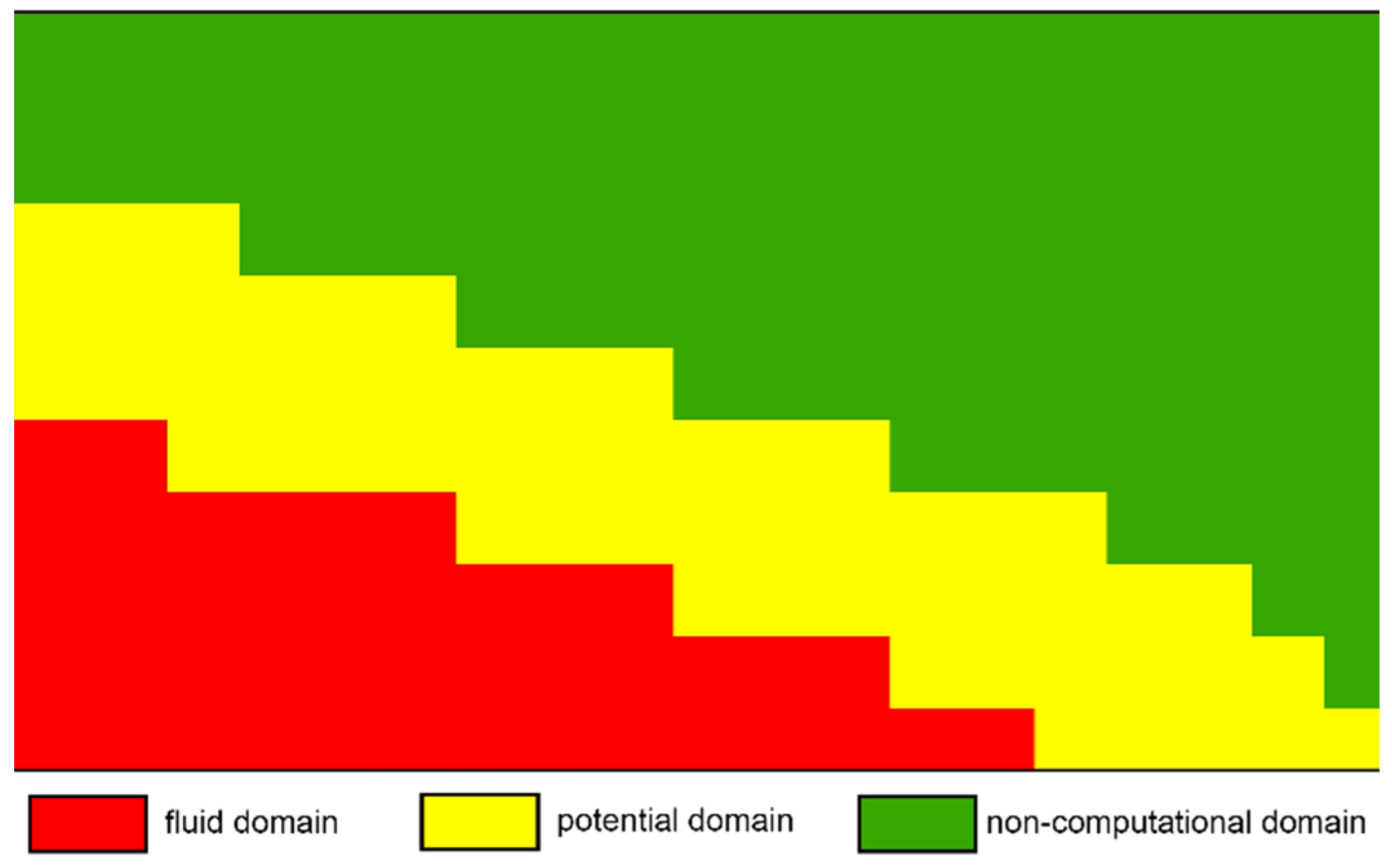
where $\odot$ denotes element-wise multiplication. This treatment plays a role similar to a localized computational stencil in conventional finite-difference or finite-volume schemes: it prevents isolated non-zero predictions in dry regions, reduces the effective computational domain, and helps maintain physically meaningful mass and momentum evolution during sequential prediction (Figure 3). In this study, a 15 × 15 neighborhood mask is adopted. This size was chosen to capture local spatial interactions while maintaining computational efficiency.

2.3. Loss Function

The loss function in PI-RCN is designed to ensure that the predicted state at the next time level satisfies the governing equations while remaining smooth and globally mass-consistent. The total loss is defined as

$$\mathcal{L}={\lambda }_h{\mathcal{L}}_h+{\lambda }_{hu}{\mathcal{L}}_{hu}+{\lambda }_{hv}{\mathcal{L}}_{hv}+{\lambda }_{TV}{\mathcal{L}}_{TV}+{\lambda }_{mass}{\mathcal{L}}_{mass}$$

(10)

where $L_h$, $L_{hu}$, and $L_{hv}$ denote the residual losses associated with the continuity, $x$-momentum, and $y$-momentum equations, respectively; $L_{TV}$ is a total-variation regularization term used to suppress spurious oscillations; and $L_{mass}$ enforces global mass conservation. The coefficients ${\lambda }_h$, ${\lambda }_{hu}$, ${\lambda }_{hv}$, ${\lambda }_{TV}$, and ${\lambda }_{mass}$ are non-negative weighting parameters that balance the relative contributions of the five loss components during training. This formulation is consistent with the implementation, where the total loss is computed as the weighted sum of the three PDE residual losses, TV loss, and mass loss.

(1)

PDE residual loss

The physical loss is constructed from the depth-averaged continuity and momentum equations. The governing system can be written in a conservative form:

$$\begin{array}{c}\begin{array}{c}{\displaystyle \frac{\partial h}{\partial t}}+\nabla \cdot \left(h\mathbf{u}\right)=0\\ {\displaystyle \frac{\partial \left(h\mathbf{u}\right)}{\partial t}}+\nabla \cdot \left(h\mathbf{u}\otimes \mathbf{u}\right)=h\mathbf{S}\end{array}\end{array}$$

(11)

where $\mathbf{u}$ is the depth-averaged horizontal velocity vector and $\mathbf{S}$ denotes the source term induced by gravity, topographic slope, internal stress, and basal friction. To improve temporal accuracy, PI-RCN employs a fully implicit time integration framework based on a mixed BDF₁/BDF₂ scheme in order to enhance numerical stability.

Let $R_h$, $R_{hu}$, and $R_{hv}$ denote the residuals of the continuity, x-momentum, and y-momentum equations evaluated at the predicted state. The corresponding residual losses are defined as

$$\begin{array}{c}\begin{array}{c}{\mathcal{L}}_h={\displaystyle \frac{1}{N}}\sum _{\left(i,j\right)\in {\mathsf{\Omega }}_a}{R}_h(i,j{)}^2\\ L_{hu}={\displaystyle \frac{1}{N}}\sum _{\left(i,j\right)\in {\mathsf{\Omega }}_a}{R}_{hu}(i,j{)}^2\end{array}\\ {\mathcal{L}}_{hv}={\displaystyle \frac{1}{N}}\sum _{\left(i,j\right)\in {\mathsf{\Omega }}_a}{R}_{hv}(i,j{)}^2\end{array}$$

(12)

where ${\mathsf{\Omega }}_a$ denotes the active computational region determined by the neighborhood mask introduced in Section 2.2, and $N$ is the number of valid cells in that region. $R_h$, $R_{hu}$, and $R_{hv}$ denote the residuals of the mass conservation equation and the momentum conservation equations in the x- and y-directions, respectively. Their temporal terms are discretized in a unified form by a mixed BDF₁/BDF₂ operator $\delta t$, written as

$$\begin{array}{c}{R}_h^{n+1}={\delta }_t{h}^{n+1}+{\displaystyle \frac{\partial (hu{)}^{n+1}}{\partial x}}+{\displaystyle \frac{\partial (hv{)}^{n+1}}{\partial y}}\\ R_{hu}^{n+1}={\delta }_t{(hu)}^{n+1}+{\displaystyle \frac{\partial F_x^{n+1}}{\partial x}}+{\displaystyle \frac{\partial G_x^{n+1}}{\partial y}}-S_x^{n+1}\\ R_{hv}^{n+1}={\delta }_t{(hv)}^{n+1}+{\displaystyle \frac{\partial F_y^{n+1}}{\partial x}}+{\displaystyle \frac{\partial G_y^{n+1}}{\partial y}}-S_y^{n+1}\end{array}$$

(13)

where

$${\delta }_t{\varphi }^{n+1}=\{\begin{array}{cc}{\displaystyle \frac{{\varphi }^{n+1}-{\varphi }^n}{\mathsf{\Delta }t}},& \mathrm{for} \mathrm{the} \mathrm{first} \mathrm{step} ({BDF}_1)\\ {\displaystyle \frac{3{\varphi }^{n+1}-4{\varphi }^n+{\varphi }^{n-1}}{2\mathsf{\Delta }t}},& \mathrm{for} \mathrm{subsequent} \mathrm{steps} ({BDF}_2)\end{array}$$

(14)

In this way, BDF₁ is used to provide a stable initialization when only one previous state is available, while BDF₂ is adopted thereafter to improve temporal accuracy during sequential time marching.

(2)

Total variation loss

In addition to the PDE residual terms, a total variation regularization (${\mathcal{L}}_{TV}$) is introduced to suppress local oscillations and improve the spatial smoothness of the predicted fields. The implementation applies TV regularization separately to h, hu, and hv, and compares the predicted field with the previous time-level field. The regularization was applied to the conservative variables $h$, $hu$, and $hv$. For a variable $q\in \left\{h,hu,hv\right\}$:

$$TV\left(q\right)={\displaystyle {\sum }_{i=1}^{N_x-1}}{\displaystyle {\sum }_{j=1}^{N_y}}\left|q_{i+1,j}-q_{i,j}\right|+{\displaystyle {\sum }_{i=1}^{N_x}}{\displaystyle {\sum }_{j=1}^{N_y-1}}\left|q_{i,j+1}-q_{i,j}\right|$$

(15)

The regularization term measures the increase in total variation from the previous state to the predicted state:

$${\mathcal{L}}_{TV}^q=max\left[TV\right(q^{n+1})-TV(q^n),0],q\in \{h,hu,hv\}$$

(16)

where $max(·)$ denotes taking the maximum value. The TV loss (${\mathcal{L}}_{TV}$) is written as

$${\mathcal{L}}_{TV}={\mathcal{L}}_{TV}^h+{\mathcal{L}}_{TV}^{hu}+{\mathcal{L}}_{TV}^{hv}$$

(17)

where each component penalizes excessive spatial variation in the corresponding predicted field. This term is especially useful for landslide dynamics because the solution often contains rapidly varying fronts, thin marginal zones, and sharp local changes in momentum. By penalizing high-frequency numerical artifacts while retaining the dominant physical structures, the TV loss improves the smoothness and robustness of the sequential prediction.

(3)

Mass conservation loss

To enforce global conservation, a mass loss is introduced based on the total flow volume before and after the update. Let $h^n$ and $h^{n+1}$ denote the thickness fields at the current and predicted time levels, respectively. The conservation loss is defined as

$${\mathcal{L}}_{mass}={\left({\displaystyle \frac{\sum _{i,j}{h}_{i,j}^{n+1}\mathsf{\Delta }x\mathsf{\Delta }y-\sum _{i,j}{h}_{i,j}^n\mathsf{\Delta }x\mathsf{\Delta }y}{\sum _{i,j}{h}_{i,j}^n\mathsf{\Delta }x\mathsf{\Delta }y+\epsilon }}\right)}^2$$

(18)

where $\mathsf{\Delta }x$ and $\mathsf{\Delta }y$ are the grid spacings and ε is a small positive constant introduced to avoid division by zero. By penalizing the relative change in total mass, ${\mathcal{L}}_{mass}$ prevents the network from producing physically implausible accumulation or loss of material during sequential propagation. This is particularly important for simulations, in which small local errors may otherwise accumulate over time and degrade the physical fidelity of the predicted landslide evolution.

The loss function combines local equation satisfaction, spatial regularity, and global conservation into a unified optimization objective. The PDE residual terms enforce the governing physics, TV regularization suppresses oscillatory artifacts, and the mass conservation term preserves the integral property of the continuity equation. These components enable PI-RCN to achieve stable and physically consistent predictions of strongly nonlinear depth-averaged landslide motion.

3. Results

All simulations were run on a local workstation using Docker with the NVIDIA JAX image nvcr.io/nvidia/jax:25.04-py3. The workstation was equipped with a 12th Gen Intel(R) Core(TM) i9-12900K CPU at 3.20 GHz, 32 GB RAM, and an NVIDIA GeForce RTX 3080 GPU with 10 GB memory. The NVIDIA driver version was 595.97, with CUDA 13.2, and the CUDA compilation tools were CUDA 12.9.

3.1. 1+1D Simulation

The one-dimensional (1+1D) frictionless dam-break flow is a canonical benchmark problem that has been used to evaluate the accuracy, stability, and robustness of numerical schemes for hyperbolic conservation laws. Owing to its well-defined wave structure and the availability of an analytical solution, this problem provides valuable insight into the performance of numerical methodologies within depth-averaged flow frameworks.

For the one-dimensional (1+1D) frictionless dam-break problem, the flow is driven solely by gravity. The governing equations are the one-dimensional depth-averaged shallow water equations without friction, expressed as follows:

$${\displaystyle \frac{\partial h}{\partial t}}+{\displaystyle \frac{\partial hu}{\partial x}}=0$$

(19)

$${\displaystyle \frac{\partial hu}{\partial t}}+{\displaystyle \frac{\partial {hu}^2+0.5g{h}^2}{\partial x}}=0$$

(20)

where $h$ denotes the water depth, $u$ is the depth-averaged velocity, and $g$ is the gravitational acceleration.

The idealized configuration consists of an infinitely extended reservoir separated by a dam located at $x=0$. Initially, the upstream water depth is prescribed as $h_0=1$, and the dam is instantaneously removed at $t=0$, generating a right-propagating positive surge and a left-propagating rarefaction wave. This configuration represents a standard Riemann problem for the shallow-water equations without friction. In the present study, both the proposed PI-RCN model and a conventional fully connected PINN are employed to solve this problem, while the analytical solution of Stoker (1992) [40] is used as the reference benchmark for quantitative comparison. The PINN baseline is implemented as a feed-forward network that maps the space–time coordinates $\left(x,t\right)$ to the flow variables $\left(h,u\right)$. The main architectural and computational settings for PINN and PI-RCN are shown in

Table 2. Main architectural and computational settings for PINN and PI-RCN.

Item	PINN	PI-RCN
Input	(x,t)	Grid
Main structure	4 hidden layers, 128 neurons each	3 blocks, 32 channels
Main operator	Dense layer	Depth-wise separable convolution
Activation function	tanh	tanh and ReLU
Optimizer	Adam	AdamW
Learning rate	$1.0\times {10}^{-4}$	$1.0\times {10}^{-3}$

.

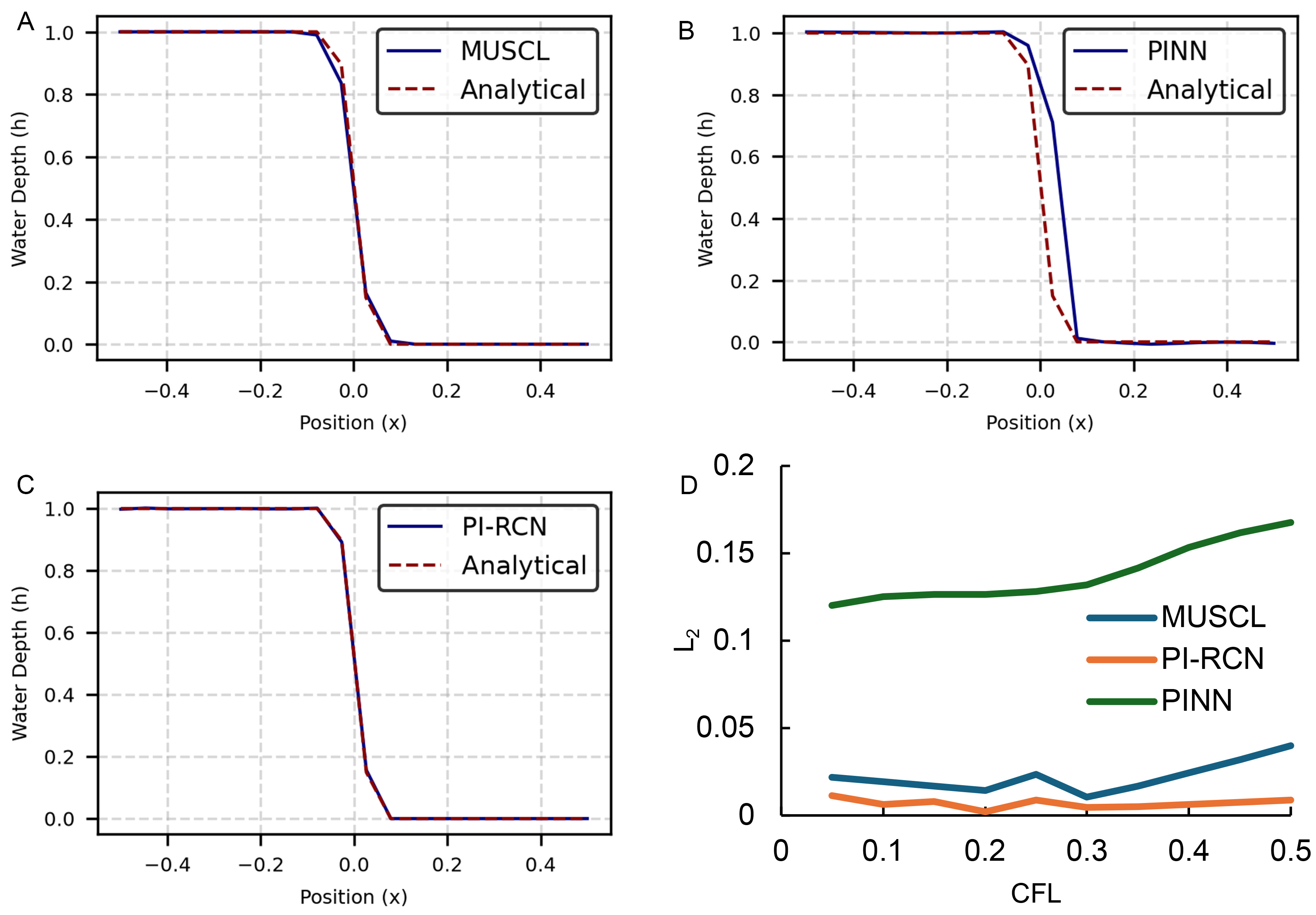
Figure 4 presents the predicted results at $t=0.01$ s, including the Monotonic Upstream-centered Scheme for Conservation Laws (MUSCL) solution, the PINN solution, the PI-RCN solution, and the corresponding L₂ loss comparison under different CFL numbers. The comparison shows that both the conventional numerical scheme and PI-RCN reproduce the overall wave structure of the dam-break flow, whereas the PINN exhibits larger deviations, particularly in regions associated with steep gradients and discontinuity-like behavior. This result is consistent with the known difficulty of conventional PINNs in resolving non-smooth features, because their solution representation is inherently smooth and their residual construction relies on differentiability. For discontinuous or sharp-gradient regions, such as moving fronts, conventional PINNs usually require more collocation points to accurately evaluate the physical residuals. The loss weights for the governing equations, boundary conditions, and data terms also need to be carefully adjusted. Otherwise, the network may mainly fit smooth regions and fail to capture abrupt changes in the solution.

The proposed PI-RCN exhibits more favorable behavior with regard to this benchmark: by learning the incremental evolution of the conservative state through a residual convolutional architecture, it more effectively represents the transient wave propagation and steep local gradients than the conventional PINN. The result of PI-RCN was obtained at CFL = 0.2, where the $L_2$ error was 0.0020, compared with 0.0143 for MUSCL and 0.1263 for PINN. These results indicate that PI-RCN can serve as an exploratory physics-informed framework for depth-averaged landslide dynamics, producing predictions that are broadly comparable to those of the traditional MUSCL scheme.

Averaged over all CFL numbers, the computational time of PI-RCN was approximately 1.24 s, which was much lower than that of PINN at 10.14 s. This indicates that PI-RCN achieved about an 8-fold speedup over the PINN while retaining the neural network-based modeling framework. The average computational time of the MUSCL solver was 0.019 s, reflecting the lower cost of the conventional numerical solver in this small one-dimensional benchmark. Nevertheless, compared with PINN, PI-RCN significantly reduced the computational burden.

3.2. 2+1D Simulation

To assess the performance of PI-RCN in more realistic two-dimensional settings, two 2+1D landslide simulations are considered. A Hong Kong landslide is used as an ablation benchmark to evaluate the respective roles of residual connections and DSCs in training stability and convergence efficiency. The Yigong rock avalanche is then employed as a large-scale real-world case to examine the ability of the proposed framework to reproduce complex spatiotemporal evolution, velocity variation, and long-runout behavior under highly nonlinear conditions. These two cases provide evidence for the optimization robustness and practical applicability of PI-RCN in depth-averaged geophysical mass-flow modeling.

In the 2+1D simulation, $\mathbf{S}$ denotes the source terms in the x- and y-directions, which are given by:

$$\begin{array}{c}{s}_x=-g_x-{\beta }_x{\displaystyle \frac{\partial h}{\partial x}} - g_z\cdot {\displaystyle \frac{u}{\left|\mathbf{u}\right|}}tan\delta \\ s_y=-g_y-{\beta }_y{\displaystyle \frac{\partial h}{\partial y}} - g_z\cdot {\displaystyle \frac{v}{\left|\mathbf{u}\right|}}tan\delta \end{array}$$

(21)

where ${\beta }_x$ and ${\beta }_y$ are the parameters related to the earth pressure coefficients. To ensure scale consistency, the equations are non-dimensionalized as: $\tilde{h}=h/H$, $\tilde{z}=z/H$, $\tilde{t}=t/T$, $\tilde{\mathbf{x}}=\mathbf{x}/L$, and $\tilde{\mathbf{u}}=\mathbf{u}/U$, where $U=\sqrt{gH}$ and ${\mu }_m={\displaystyle \frac{L}{H}}·tan\delta$. Accordingly, the governing equations can be written as follows:

$${\displaystyle \frac{\partial }{\partial t}}\left[\begin{array}{c}\tilde{h}\\ \tilde{h}\tilde{u}\\ \tilde{h}\tilde{v}\end{array}\right]+\nabla \cdot \left[\begin{array}{cc}\tilde{h}\tilde{u}& \tilde{h}\tilde{v}\\ \tilde{h}{\tilde{u}}^2+{\displaystyle \frac{1}{2}}{k}_{a/p}{\tilde{h}}^2& \tilde{h}\tilde{u}\tilde{v}\\ \tilde{h}\tilde{u}\tilde{v}& \tilde{h}{\tilde{v}}^2+{\displaystyle \frac{1}{2}}{k}_{a/p}{\tilde{h}}^2\end{array}\right]=\left[\begin{array}{c}0\\ -{\displaystyle \frac{d\tilde{z}}{dx}}-{\displaystyle \frac{\tilde{u}}{\tilde{\mathbf{u}}}}\cdot {\mu }_m\\ -{\displaystyle \frac{d\tilde{z}}{dy}}-{\displaystyle \frac{\tilde{v}}{\tilde{\mathbf{u}}}}\cdot {\mu }_m\end{array}\right]$$

(22)

where $\nabla \cdot$ is a divergence operator acting on the flux tensor. $u={\left(u,v\right)}^T$ denotes the depth-averaged horizontal velocity vector, where $u$ and $v$ are the components in the $x$- and $y$-directions, respectively. The active and passive earth pressure coefficients, $k_a$ and $k_p$, describe the redistribution of normal stress caused by the internal friction of the moving granular mass. Specifically, $k_a$ is used when the material is in an extensional state, whereas $k_p$ is used when the material is in a compressional state. They are defined as

$$k_{a/p}=2{\mathrm{s}\mathrm{e}\mathrm{c}}^2\varphi \cdot \left(\begin{array}{c}1\mp \sqrt{1-{\mathrm{c}\mathrm{o}\mathrm{s}}^2\varphi {\mathrm{s}\mathrm{e}\mathrm{c}}^2\delta }\end{array}\right)-1$$

(23)

where $\varphi$ is the internal friction angle and $\delta$ is the basal friction angle.

To ensure the continuity and differentiability of the earth pressure coefficient, thereby improving training stability and facilitating convergence, a smooth transition between the active and passive states is introduced:

$$k=k_a+\left(k_p-k_a\right)\cdot sigmoid\left(-{\displaystyle \frac{\partial u}{\partial x}}\right)$$

(24)

(1)

Hong Kong landslide

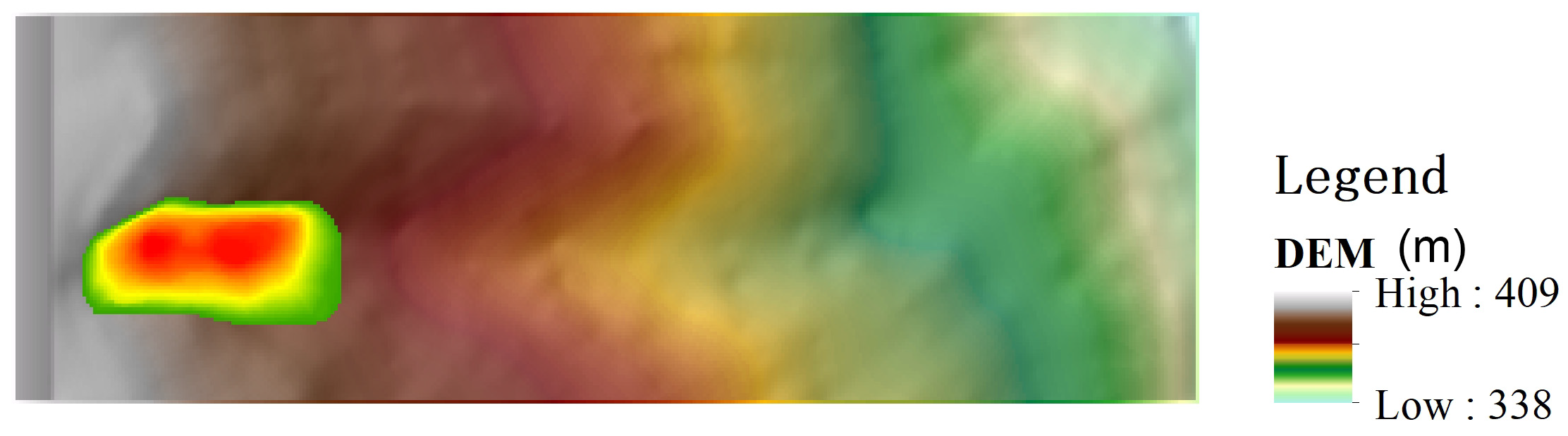
A well-documented landslide event that occurred in 1993 in Lantau Island, Hong Kong, is adopted to evaluate the proposed method under realistic topographic and source conditions [41]. The digital elevation model (DEM) and source data were derived from the work of Ouyang et al. [24] (Figure 5), and the landslide motion is simulated within the Savage–Hutter framework [5], with an internal friction angle of 20° and a basal friction angle of 16°. The PI-RCN parameters are listed in

Table 3. Key PI-RCN settings for the Hong Kong landslide case.

Parameter	Setting
Feature channels/residual blocks	32/4
Convolution kernel	7 × 7
CFL	0.6
Time-step range	$1.0 \times {10}^{-4}$–1 s
Neighborhood mask	15 × 15
Total simulation time	12 s
Loss weights	$w_h=1;$$w_{hu}=10;$$w_{hv}=10;$$w_{TV}=1.0\times {10}^{-6};$$w_{mass}=1.0\times {10}^{-3}$

.

This case is used here not primarily as a final predictive benchmark, but as a controlled test for examining how different architectural choices affect the convergence behavior.

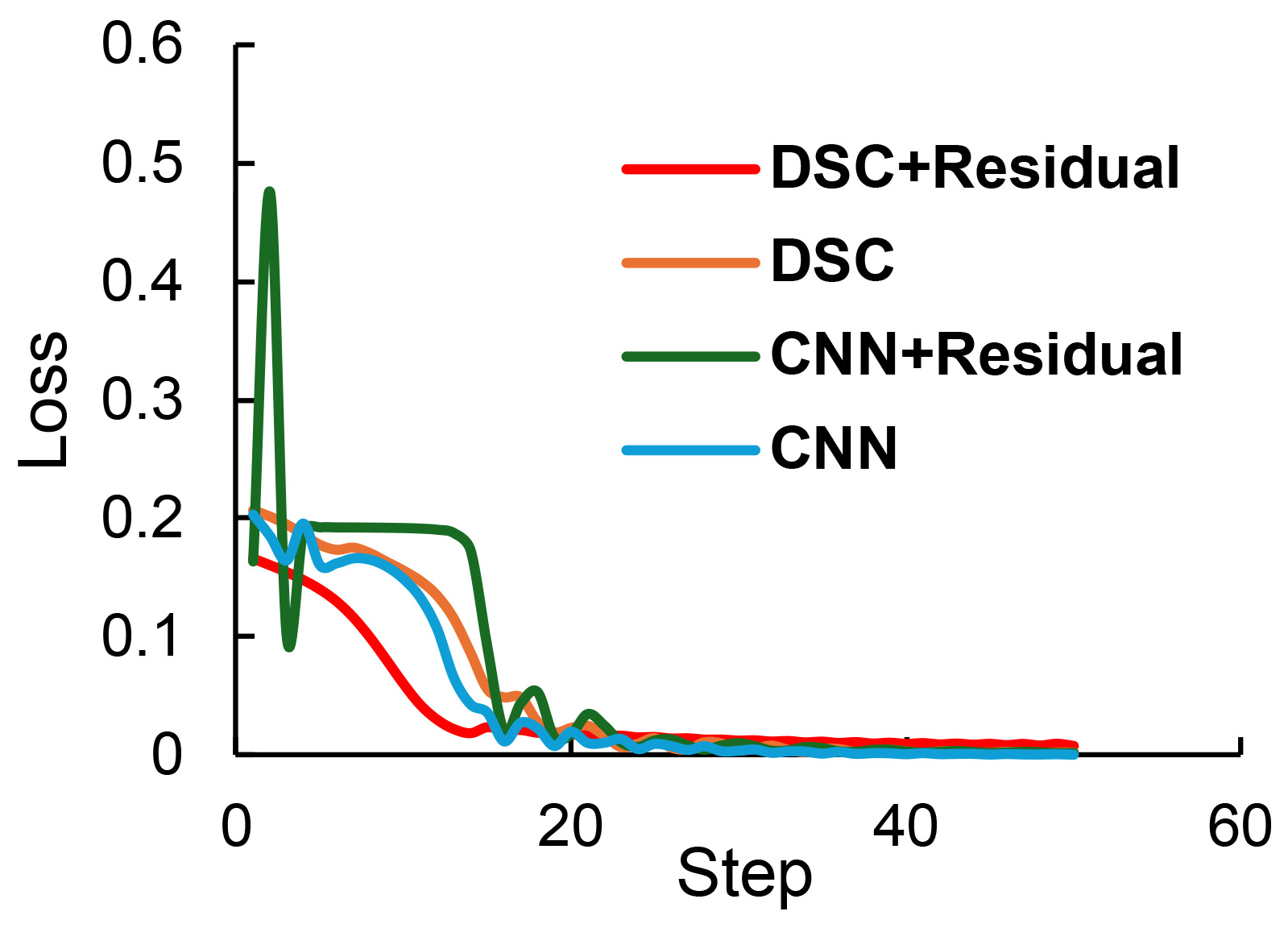
Figure 6 shows the training loss histories of four network variants: DSC+Residual, DSC, CNN+Residual, and CNN. The DSC-based models (DSC+Residual and DSC) each contain 21,654 trainable parameters, whereas the CNN-based models (CNN+Residual and CNN) each contain 79,587 trainable parameters. Although the four models start from comparable initial losses at Step 1, their subsequent optimization trajectories differ markedly. In particular, the CNN+Residual configuration exhibits pronounced early-stage instability, with the loss increasing sharply to 0.476 at Step 2, whereas the other three architectures show a monotonic decrease during the first ten training steps.

Among the tested variants, the DSC+Residual architecture achieves fast and stable convergence. Its loss decreases to 0.059 by Step 10 and remains the lowest during the intermediate stage, reaching 0.017 at Step 20, compared with 0.023 for DSC, 0.0170 for CNN+Residual, and 0.0204 for CNN. In the later stage, all four models converge to losses below 0.01, but DSC+Residual maintains a consistent optimization trajectory throughout the full training process. These results indicate that the DSC+Residual architecture achieved performance comparable to the other tested architectures while using substantially fewer trainable parameters. Specifically, depth-wise separable convolution reduced the parameter number from 79,587 to 21,654. Therefore, the DSC+Residual architecture provides a more compact model structure while retaining effective local feature extraction capabilities.

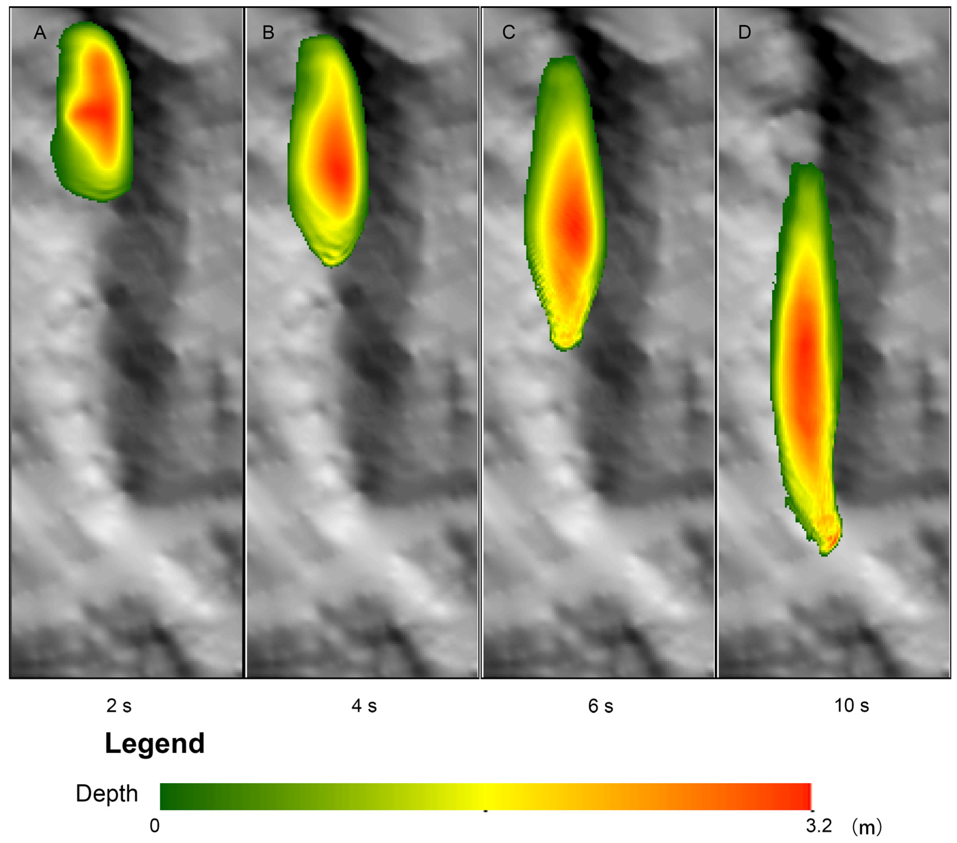
The improved optimization behavior is also reflected in the predicted landslide evolution. As shown in Figure 7, the PI-RCN simulation reproduces a clear and continuous downslope propagation of the sliding mass. To evaluate the predictive accuracy of the proposed model, the PI-RCN results were compared with the finite volume with Van Leer splitting method (FV-VLS) solution at several representative times (2 s, 4 s, 6 s, and 10 s). The corresponding L₂ errors are 0.012 m² at t = 2, 0.006 m² at t = 4, 0.011 m² at t = 6, and 0.025 m² at t = 10. These results indicate that PI-RCN maintains good agreement with FV-VLS. Moreover, these spatiotemporal characteristics are consistent with the evolution pattern reported by Chen and Lee (2003) [41].

(2)

Yigong rock avalanche

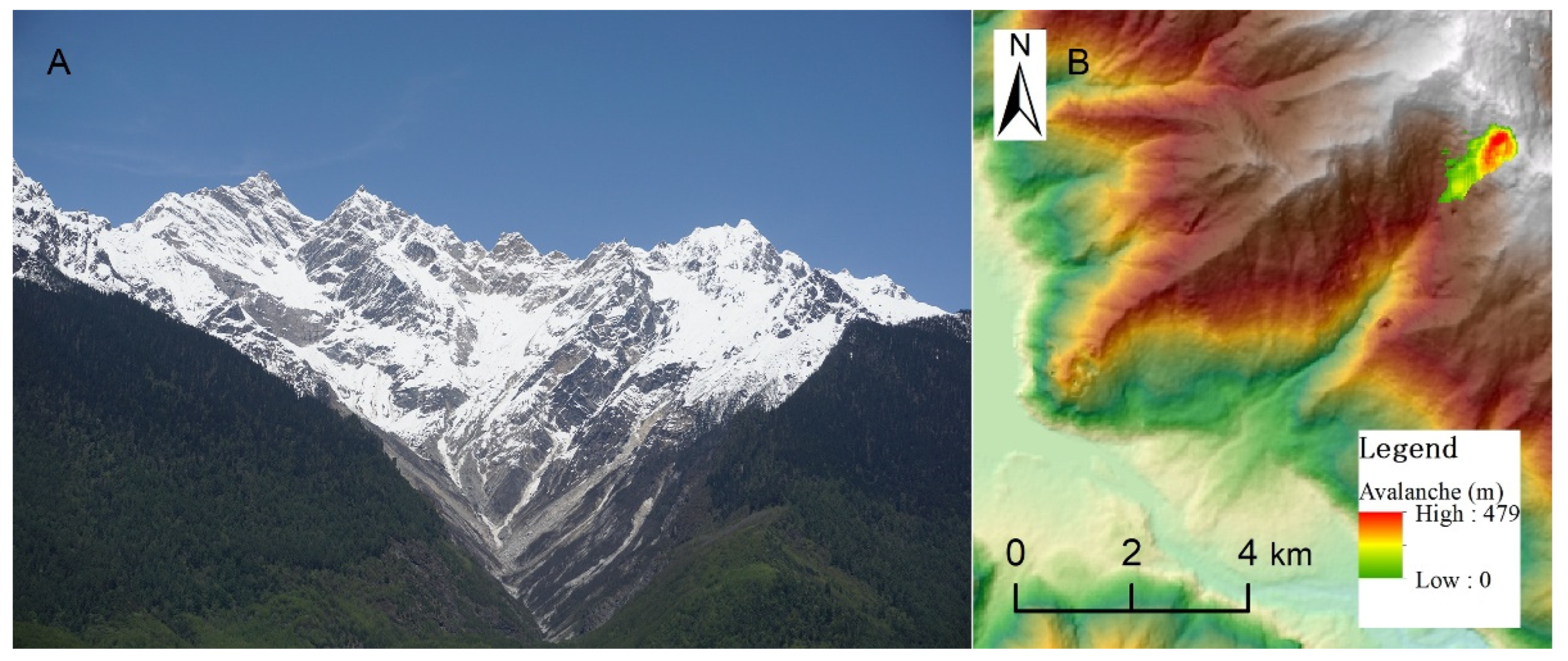
The Yigong rock avalanche is employed as a real-world large-scale benchmark to evaluate the practical applicability of PI-RCN to high-energy, long-runout geophysical mass flows. This event (94°58′03″ E, 30°12′11″ N) occurred on 9 April 2000 in the Yigong Tsangpo Valley of southeastern Tibet and involved an estimated 3 × 10⁸ m³ of rock that detached from a steep source area, traveled several kilometers downslope at high velocity, and ultimately dammed the Yigong Tsangpo River (Figure 8). Owing to its large volume, rapid motion, and complex runout process, the event provides a challenging test case for the proposed framework. In the present simulation, the avalanche is modeled using the Savage–Hutter equations with an internal friction angle of 24° and a basal friction angle of 20°, and the source height is obtained from the Massflow software package (V2.0). The parameters in PI-RCN are shown in

Table 4. Key PI-RCN settings for the Yigong landslide case.

Parameter	Setting
Feature channels/residual blocks	32/4
Convolution kernel	7 × 7
CFL target	0.2
Time-step range	1.0 × 10−4–1 s
Neighborhood mask	15 × 15
Total simulation time	100 s
Loss weights	$w_h=1;$$w_{hu}=0.1;$$w_{hv}=0.1;$$w_{TV}=1.0\times {10}^{-7};$$w_{mass}=1$

.

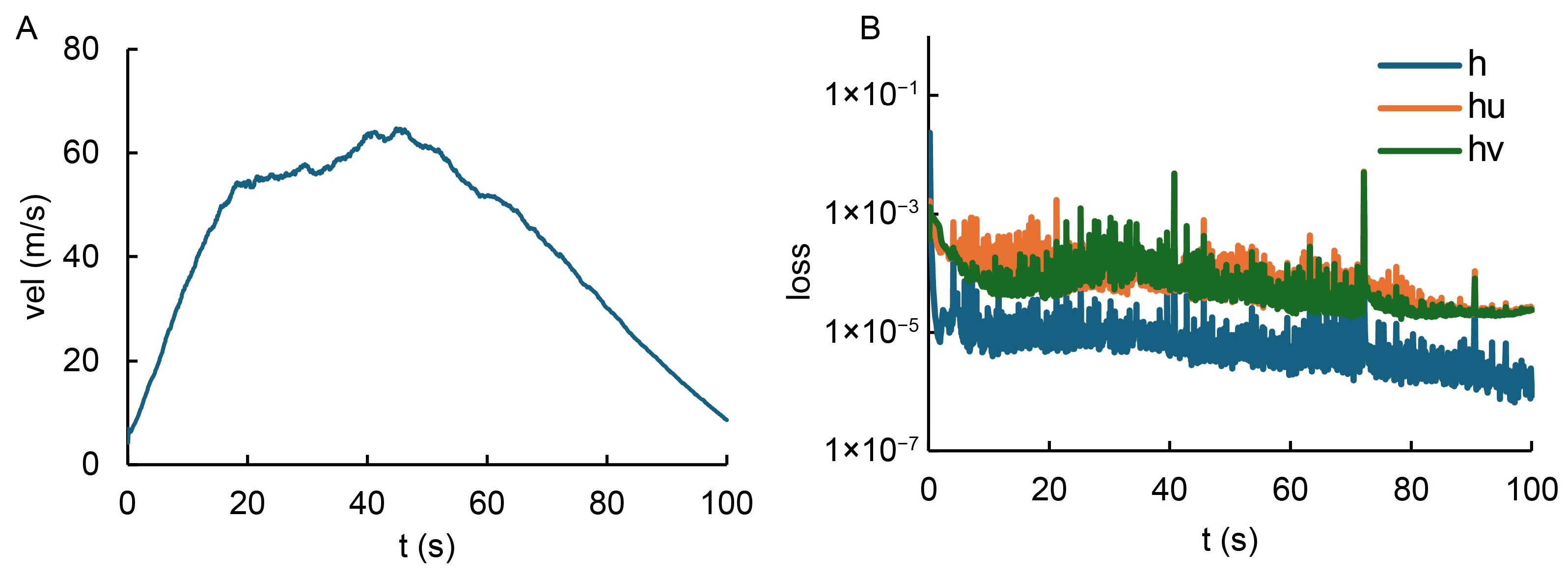
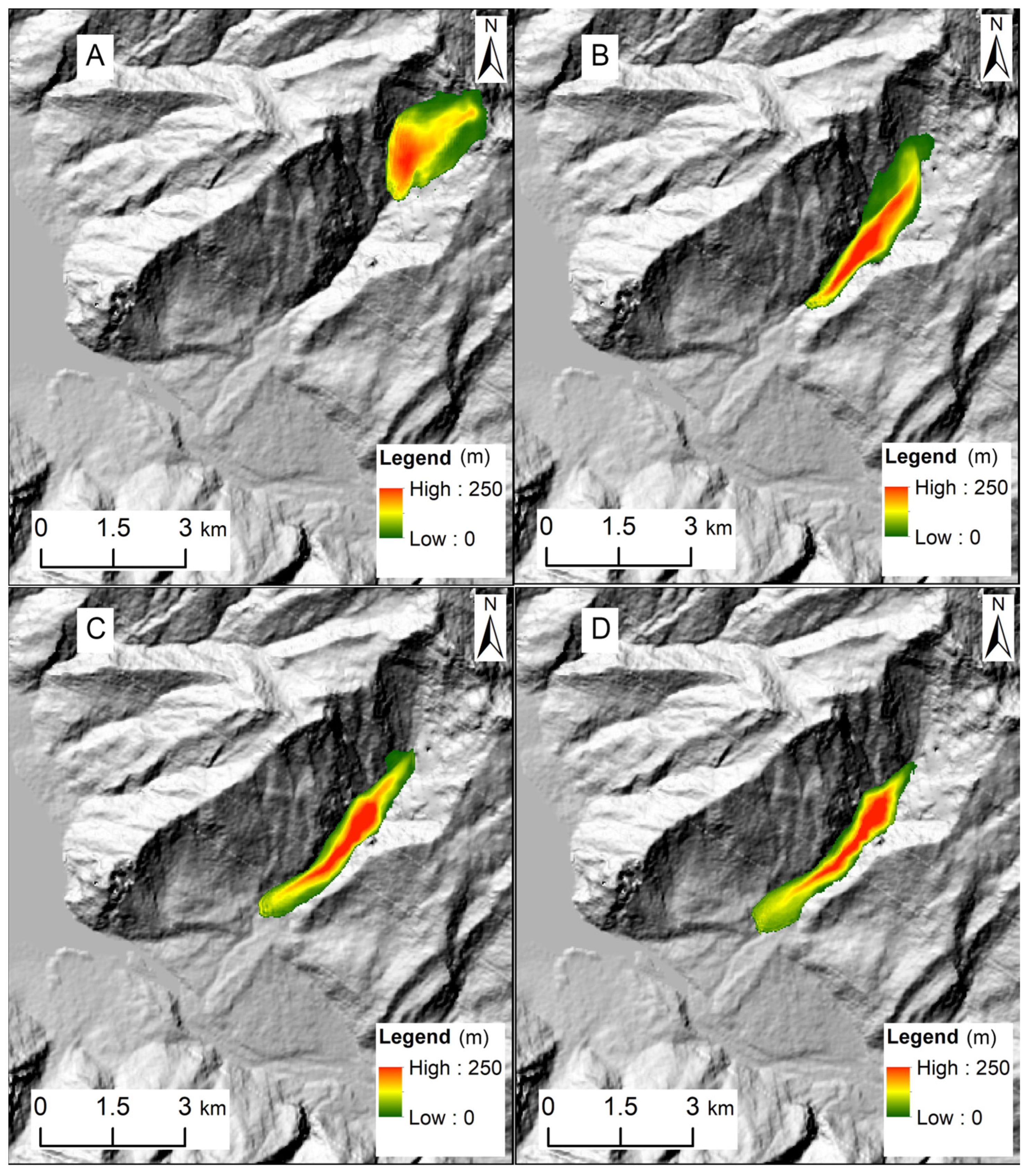
The predicted kinematic evolution is shown in Figure 9A and Figure 10. The rapid movement phase lasts approximately 80–100 s, which is consistent with the timescale reported in previous studies. At 20 s, the avalanche remains concentrated near the source area and corresponds to the early acceleration stage. By 40 s, the flow enters the peak-velocity stage and exhibits pronounced downslope elongation, with a velocity of approximately 60–70 m/s. At 60 s, the avalanche reaches its greatest runout extent, representing a quasi-steady high-momentum stage. By 80 s, the front decelerates and the deposit begins to thicken, indicating progressive momentum dissipation and deposition. The result suggests that PI-RCN is able to reproduce the major stages of realistic avalanche motion, including acceleration, peak transport, long-runout propagation, and deceleration.

Figure 9B shows the temporal behavior of the loss components associated with the depth and momentum conservation equations. Although minor short-term fluctuations are observed, all residual terms decrease rapidly by several orders of magnitude during the early training stage and subsequently stabilize within the range of 10⁻³ to 10⁻⁶. This sustained decay indicates that mass and momentum conservation are effectively enforced during training and provides evidence that the proposed framework remains numerically stable even for highly energetic avalanche dynamics.

The Yigong case further demonstrates the potential of PI-RCN as an AI-driven framework for simulating rapid long-runout rock-avalanche motion in steep mountain valleys. The predicted rapid acceleration, valley-confined transport, and subsequent deceleration show that the model can capture the principal stages of long-distance mass movement under strong topographic control. Relative to conventional PINN frameworks, PI-RCN better resolves the strongly nonlinear and sharply varying flow features that characterize extreme landslide motion.

The two 2+1D cases confirm the effectiveness of PI-RCN from two complementary perspectives. The Hong Kong landslide shows that the DSC-Residual architecture improves convergence behavior and suppresses optimization instability, whereas the Yigong case demonstrates that the same framework can reproduce physically realistic spatiotemporal evolution and velocity characteristics in a real large-scale hazard scenario. These findings suggest the potential of PI-RCN as a compact and physics-informed network for nonlinear geophysical mass-flow simulation.

4. Discussion

The results of the benchmark indicate that the proposed PI-RCN framework provides a practical improvement over conventional PINN-based approaches for depth-averaged landslide simulation. The main advantage of the method does not lie in replacing established shock-capturing solvers, but in offering a more efficient and stable physics-informed model for strongly nonlinear spatiotemporal flow problems. The present results suggest that the combination of residual learning and DSCs addresses two key limitations of conventional PINNs in geophysical mass-flow modeling, namely optimization instability and high computational cost.

A reason for the improved performance of PI-RCN is the residual time-marching formulation. Instead of reconstructing the entire flow state independently at each step, the network learns the incremental evolution between two adjacent time levels. This design reduces the learning burden of each forward pass because consecutive landslide states are strongly correlated in time, and their differences are generally smoother than the full solution field. The benchmark dam-break results support this interpretation: PI-RCN reproduces the analytical solution with high accuracy, indicating that the structure is effective.

The Hong Kong ablation study further clarifies the complementary roles of the two architectural components. Residual connections primarily improve gradient propagation and stabilize deep optimization, whereas DSCs reduce parameter count and computational cost while preserving the ability to extract localized spatial features. Their combination leads to the most favorable training behavior among the tested variants.

PI-RCN is particularly suitable for depth-averaged flow systems in which nonlinear transport, topographic forcing, and frictional source terms interact over many sequential time steps. In the Yigong rock avalanche, the framework remains stable while reproducing the spatiotemporal evolution, multi-stage velocity pattern, and realistic long-runout behavior of the avalanche. The sustained decay of the governing-equation residuals suggests that the model is able to preserve the main physical constraints, even in a rapidly evolving flow regime. This is a meaningful property for practical geohazard simulation.

In addition, PI-RCN improves the trainability and efficiency of physics-informed learning for nonlinear depth-averaged flow systems by combining residual evolution modeling with parameter-efficient convolutional feature extraction. PI-RCN is an exploratory attempt to develop a residual time-marching framework. The dam-break benchmark, Hong Kong case, and Yigong case together suggest that the framework can provide physically consistent predictions and improved computational efficiency relative to a baseline PINN. Future work should further extend this framework to erosion–entrainment processes, complex rheology, and more rigorous validation using field observations.

5. Conclusions

This study developed a physics-informed residual convolutional network (PI-RCN) for depth-averaged landslide dynamics and evaluated it using a benchmark dam-break problem, a Hong Kong landslide, and the Yigong rock avalanche. These results indicate that PI-RCN shows potential as a neural-network-based tool for supporting engineering-geological studies of landslide dynamics, especially where rapid evaluation of runout behavior, topographic control, and hazard implications is required. Compared with a baseline PINN, PI-RCN provides an efficient and robust route for physics-informed simulation of transient landslide motion.

By applying the framework to real landslide cases over complex terrain, we show that PI-RCN can reproduce terrain-guided propagation, local confinement effects, long-runout behavior, and multi-stage velocity evolution that are directly relevant to engineering-geological interpretation. In this sense, the proposed framework offers a practical bridge between physics-informed network modeling and hazard-oriented analysis of landslide mobility.