1. Introduction
High-resolution seismic processing is essential for identifying thin beds, stratigraphic pinch-outs, subtle faults, and weak discontinuities. In practice, however, recorded seismic traces are band-limited and their high-frequency components are further weakened by source bandwidth, acquisition geometry, environmental noise, and propagation attenuation associated with the Q factor. These effects reduce the effective frequency bandwidth of the wavelet and therefore degrade the vertical resolution of seismic data.
Over the past several decades, a variety of methods have been developed to enhance seismic resolution. Robinson introduced the classical convolution model [
1], in which a seismic trace is represented as the convolution of a seismic wavelet with a reflection coefficient sequence. Based on this model, predictive deconvolution, adaptive deconvolution, Gabor deconvolution, and related time-varying spectral compensation methods were proposed to recover high-frequency components from band-limited observations [
2,
3,
4]. Although these methods can sharpen seismic wavelets to some extent, they often rely on restrictive assumptions such as stationary or minimum-phase wavelets and white reflectivity, which are difficult to satisfy in complex geological environments.
To compensate for attenuation and phase distortion during wave propagation, inverse-
Q filtering and related attenuation compensation strategies have also been extensively investigated [
5,
6,
7,
8,
9,
10]. These methods can partially restore high-frequency content, especially in deep formations, but their performance is sensitive to noise and to errors in the attenuation model. As a result, strong high-frequency amplification may introduce unstable amplitudes or reconstruction artifacts.
In recent years, deep learning has provided an alternative data-driven route for seismic resolution enhancement because neural networks can learn nonlinear mappings directly from large datasets rather than depending completely on explicit signal assumptions [
11,
12]. Optimization-inspired high-resolution inversion networks [
13], structure-constrained reconstruction models [
14], attenuation-aware vertical resolution enhancement strategies [
15], feature-aware deep enhancement models [
16], pseudo-well-driven adversarial approaches [
17], self-supervised blind deconvolution [
18], self-supervised frequency extension frameworks [
19], and non-local similarity regularization [
20] have all shown that data-driven models can recover missing high-frequency information more effectively than conventional handcrafted filters in many scenarios.
Nevertheless, three limitations remain common in the current literature. First, many supervised methods require paired low-resolution (LR) and high-resolution (HR) labels generated from wells, synthetic models, or pseudo labels, which limits adaptability to field data. Second, one-way regression models often emphasize local trace sharpening but do not explicitly constrain whether the reconstructed HR signal remains consistent with the original LR observation after reverse mapping. Third, spectral enhancement may come at the expense of structural continuity when the loss function does not directly penalize waveform distortion and reflector inconsistency.
To address these issues, this study formulates seismic resolution enhancement as a structure-preserving bidirectional translation problem between a low-bandwidth seismic domain and a high-bandwidth seismic domain. From this perspective, the proposed method should be viewed not simply as “another GAN model”, but as a bidirectional bandwidth translation framework in which cycle-consistent adversarial learning is used as the optimization mechanism. The forward mapping is responsible for recovering missing high-frequency content, whereas the reverse mapping acts as a regularizer that constrains the enhanced signal to remain physically compatible with the original low-bandwidth observation. In addition, an SSIM-based structural term is embedded in the objective function to preserve waveform morphology and reflector geometry during spectral extension.
Accordingly, the contributions of this paper can be summarized in three aspects. First, we propose a structure-preserving bidirectional bandwidth translation framework for seismic resolution enhancement, where LR-to-HR enhancement and HR-to-LR back-projection are jointly optimized to constrain spectral recovery with cycle-consistent structural regularization. Second, we design a hybrid training strategy that combines field-extracted wavelets, synthetic reflectivity construction, and a lightweight one-dimensional residual backbone, thereby improving the compatibility of the learned model with oscillatory seismic traces and real bandwidth characteristics. Third, we present a comprehensive experimental study including comparisons with conventional and recent learning-based methods, public benchmark evaluation on SEG Open Data, and extensive ablation, sensitivity, robustness, and efficiency analyses.
The remainder of this paper is organized as follows.
Section 2 presents the problem formulation, domain-construction procedure, and proposed network.
Section 3 describes the datasets, implementation details, and comparison results.
Section 4 reports ablation experiments and extended analyses. Finally,
Section 5 and
Section 6 provide the discussion and conclusion, respectively.
2. Method
2.1. Training Domain Construction
Many deep learning methods fail to generalize well when the amount of training data is insufficient. In this study, the training data are generated in a controlled yet geologically informed manner so that the model can observe sufficient bandwidth variations during optimization.
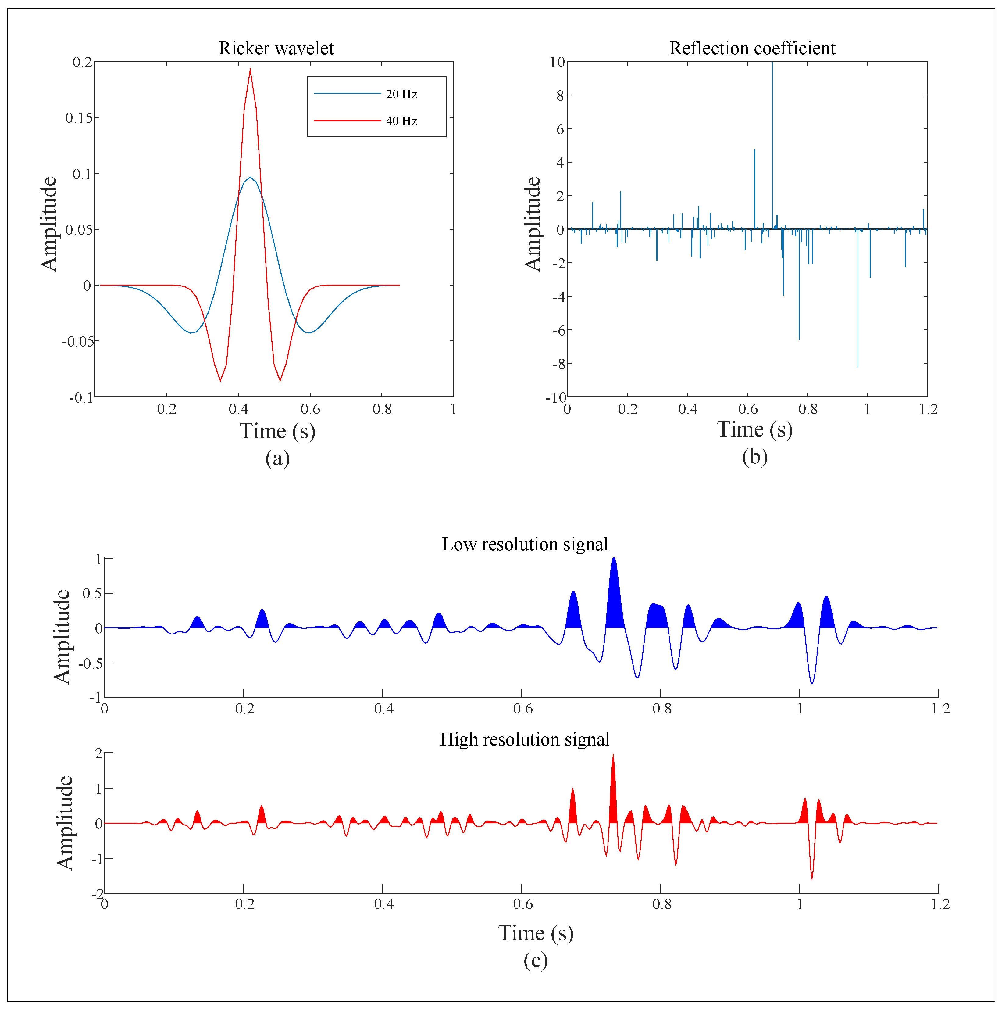
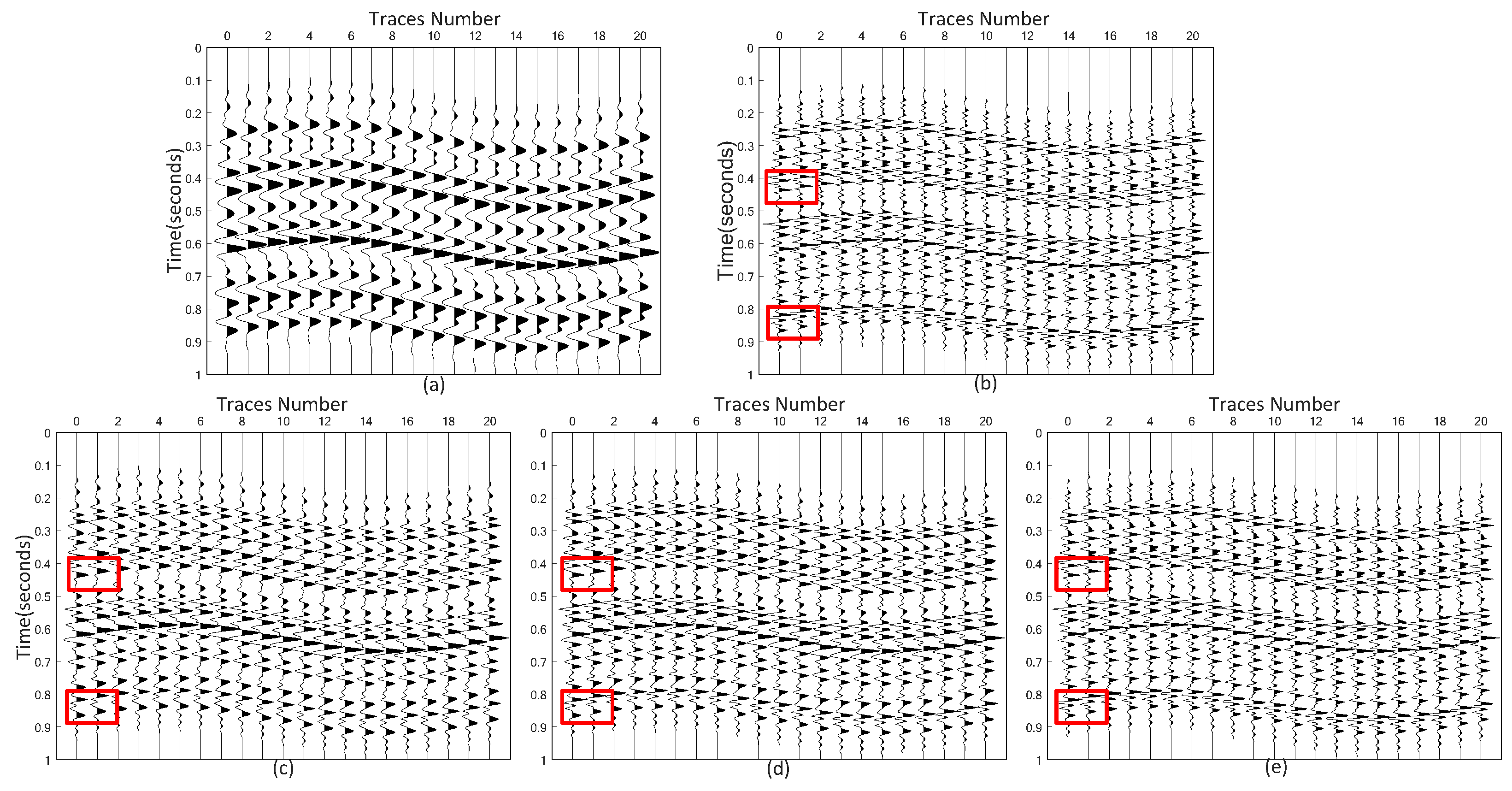
Figure 1 shows the basic principle of constructing synthetic seismic signals from wavelets and reflection coefficients.
Because the composition of field seismic data is much more complex than that of idealized synthetic examples, a pure Ricker wavelet assumption is insufficient for practical training. We therefore first extract representative wavelets from field seismic data and then use these wavelets to construct two bandwidth-controlled domains. The field-extracted wavelets are selected from laterally continuous windows with relatively high signal-to-noise ratios and stable phase characteristics. Wavelets dominated by isolated noise bursts, strong acquisition footprint, or visibly unstable phase are excluded before normalization. The remaining wavelets are grouped according to their effective frequency support, so that the domain separation is controlled by bandwidth rather than by the spatial position of the original field traces. Wavelets with effective frequency content in 10–60 Hz are used to generate the LR domain, whereas wavelets with effective frequency content in 40–80 Hz are used to generate the HR domain. For each domain, random sparse reflection coefficient sequences with varying amplitudes, layer thicknesses, and event spacing are generated independently and convolved with wavelets drawn from the corresponding wavelet pool. The LR and HR traces are therefore not paired sample by sample: a trace in the LR domain and a trace in the HR domain do not share the same reflectivity realization during unpaired adversarial training. In this way, the LR and HR corpora are statistically coupled through a shared geological prior, but remain unpaired at the trace level. Mild amplitude perturbations and additive noise are further introduced during training to improve robustness.
For all experiments, each trace contains 800 samples. The synthetic database contains 400,000 traces in total and is divided into 320,000, 40,000, and 40,000 traces for training, validation, and testing, respectively. The validation subset is used only for model selection and hyperparameter checking, while the held-out test subset is used only for the final quantitative reports. To avoid leakage, traces generated from the same random reflectivity seed are assigned to a single subset. Before being fed into the network, each trace is normalized to . This design enables the model to learn the mapping between bandwidth-limited and bandwidth-extended seismic domains while retaining the waveform and amplitude characteristics observed in real seismic data. It also keeps the training protocol consistent with the intended field application, where a clean HR label is generally unavailable for each observed LR trace.
2.2. Problem Statement and Degradation Model
Let
denote an ideal high-resolution seismic trace with sampling length
T, and let
denote the corresponding low-resolution observation. In a simplified form, the degradation from
to
can be described as the combined effect of bandwidth limitation, attenuation, acquisition footprint, and noise contamination:
where
h is a band-limiting kernel,
denotes convolution,
represents the effective acquisition-and-propagation operator, and
n denotes additive noise. In practice, the exact operator
is unknown, non-stationary, and often varies with geological setting, depth, and acquisition geometry. Therefore, seismic resolution enhancement is better interpreted as an ill-posed inverse problem than as a deterministic deblurring task.
Given an observed LR trace , the purpose of seismic resolution enhancement is to estimate an HR trace that satisfies three practical requirements simultaneously: (1) it should recover additional high-frequency information, (2) it should remain structurally consistent with the input trace, and (3) it should avoid introducing unstable oscillations or artificial reflector discontinuities. These requirements motivate the use of a coupled objective rather than a single pixel-wise or sample-wise regression loss.
2.3. Bandwidth-Domain Formulation
The proposed method reformulates seismic resolution enhancement as translation between two related but unpaired signal domains rather than direct point-to-point regression. The LR domain contains seismic traces whose dominant frequency and absolute bandwidth are restricted by attenuation and acquisition conditions. The HR domain contains traces with richer high-frequency content and sharper interference patterns. Here, the subscript “real” denotes the samples drawn from the constructed LR or HR training domain used by the discriminator; it does not imply that paired field HR labels are available. The objective of the forward generator is to recover the missing high-frequency content, whereas the reverse generator projects the enhanced result back to the LR domain and therefore acts as a consistency regularizer.
This bidirectional design is important for seismic data. If only the forward mapping is optimized, the network may overemphasize local oscillations and produce visually sharper but physically inconsistent traces. By enforcing that an enhanced trace should be convertible back to the original LR observation, the proposed framework suppresses artificial spectral gains that are unsupported by the input data. Therefore, the reverse mapping is not merely an auxiliary branch but a key mechanism for stabilizing bandwidth extension.
From an optimization perspective, the LR domain and the HR domain should not be regarded as two unrelated data manifolds. They are coupled through the same subsurface reflectivity, but differ in effective bandwidth and interference pattern. The proposed model exploits this property by learning a domain-level transformation rather than a fixed deterministic filter. This distinction is important because the same local waveform in the LR domain may correspond to different HR outcomes under different geological contexts. Domain translation allows the model to account for such ambiguity in a data-driven manner.
2.4. Structure-Preserving Bidirectional Translation Network
Generative models play an important role in image translation, synthesis, and reconstruction tasks. Goodfellow et al. introduced an adversarial training strategy for generative modeling and proposed the generative adversarial network (GAN) framework [
21]. In GAN, two neural networks, namely a generator and a discriminator, are trained simultaneously in an adversarial manner. The generator aims to produce synthetic samples that resemble the real data distribution, while the discriminator acts as a binary classifier to distinguish generated samples from real ones. Through this adversarial learning process, the two networks are optimized alternately in a minimax game until an equilibrium is reached, where the generated samples become increasingly indistinguishable from real data.
It should be noted that the adversarial architecture does not provide a closed-form analytical equation for all nonlinear dependencies in seismic traces. Instead, the generator represents a learnable nonlinear operator composed of convolutional filters, nonlinear activations, residual mappings, and normalization layers. These operations approximate nonlinear bandwidth transformation from data, while the discriminator supplies a distribution-level constraint that penalizes outputs inconsistent with the target bandwidth domain. Cycle consistency further restricts this nonlinear mapping by requiring the translated signal to be mapped back to its original domain, thereby reducing the admissible solution space and making the learned relationship more physically plausible.
CycleGAN extends the GAN framework by introducing a cycle consistency constraint, which enables bidirectional mapping between two domains without requiring paired training samples [
22]. This framework is particularly suitable for translation between correlated data domains. In seismic signal processing, resolution enhancement can be naturally interpreted as translation between LR and HR seismic domains.
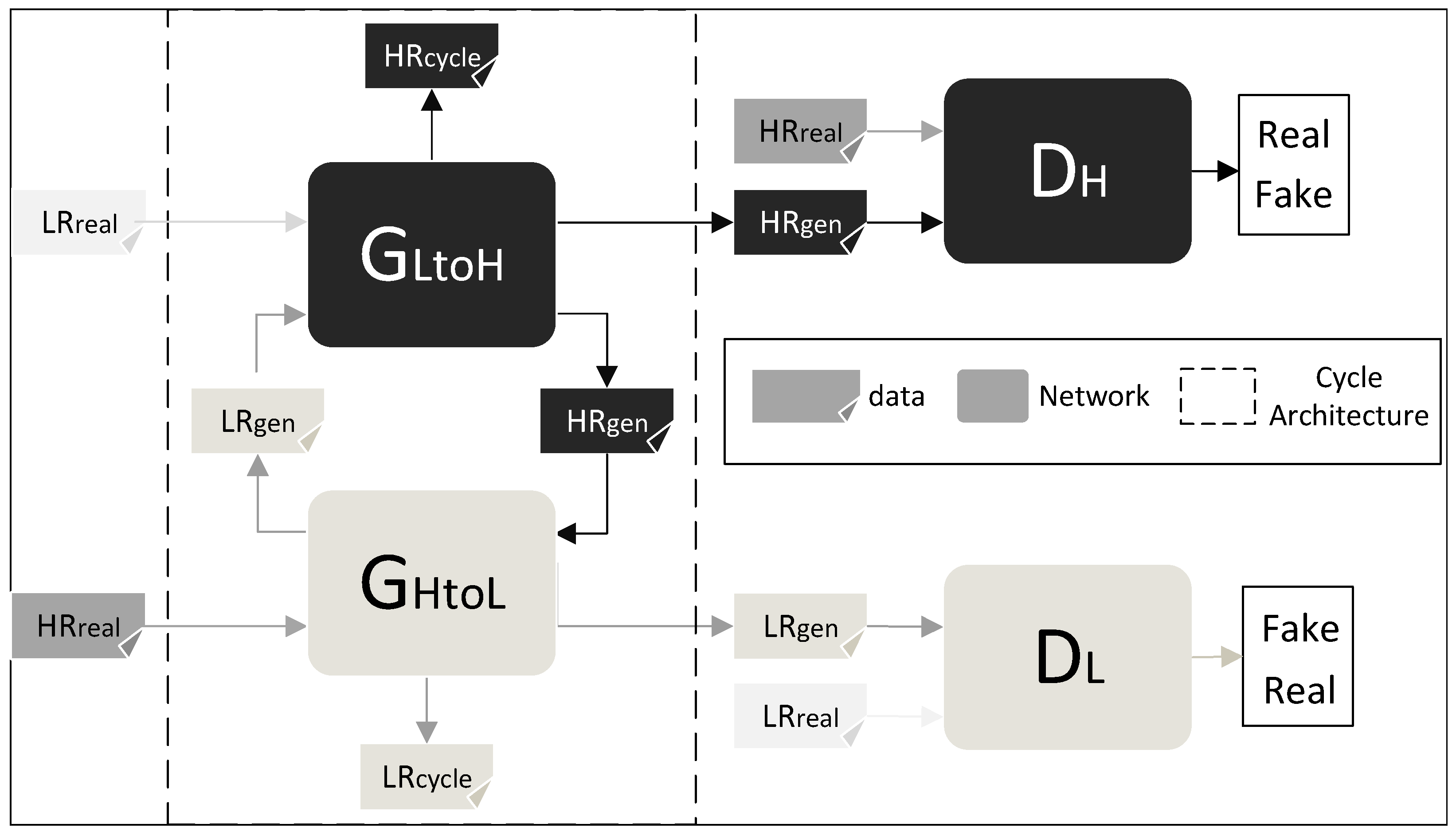
Figure 2 illustrates the overall architecture of the proposed model.
The generator
learns a mapping from the LR domain
to the HR domain
. The corresponding adversarial loss is defined as
Similarly, the generator
performs the reverse mapping from the HR domain to the LR domain, and its adversarial loss is defined as
In addition to the adversarial loss, CycleGAN introduces a cycle consistency constraint to ensure that the translated signal can be mapped back to the original domain. The cycle consistency loss is defined as
To further preserve structural information in reconstructed seismic traces, the structural similarity index (SSIM) [
23] is incorporated into the loss function. Because the proposed framework is trained on unpaired LR and HR domains, the SSIM term is applied to cycle-reconstructed traces rather than to unmatched cross-domain samples. In this way, structural preservation is enforced on sample-consistent signal pairs while the network remains fully unpaired. SSIM measures the structural similarity between two signals and is defined as
where
and
denote the mean values of signals
x and
y,
and
denote the corresponding variances, and
denotes the covariance between the two signals.
and
are small constants introduced to avoid numerical instability. The theoretical range of SSIM is from −1 to 1 when negative covariance is possible, while in most normalized reconstruction evaluations it is interpreted on the interval from 0 to 1. A value of 1 indicates identical structural information between two signals. Values closer to 1 represent higher structural similarity, values close to 0 indicate weak structural agreement, and negative values, if they occur, indicate opposite or inverted local structural correspondence.
For an LR input trace, let
denote the cycle-reconstructed signal. The corresponding structural similarity is computed as
Accordingly, the structural loss associated with the LR cycle is defined as
Similarly, for an HR input trace, let . We then compute , which leads to the structural loss .
Finally, the overall optimization objective of the network can be written as
where
and
are two trade-off coefficients, which are set to 5 and 10 in this paper. From the viewpoint of seismic resolution enhancement, the adversarial losses encourage domain-level spectral realism, the cycle consistency term constrains recoverability, and the SSIM term preserves waveform morphology and reflector geometry during cycle reconstruction. Their combination forms a coupled objective for bandwidth extension and structural preservation without requiring paired HR labels.
2.5. Structure of Generator and Discriminator
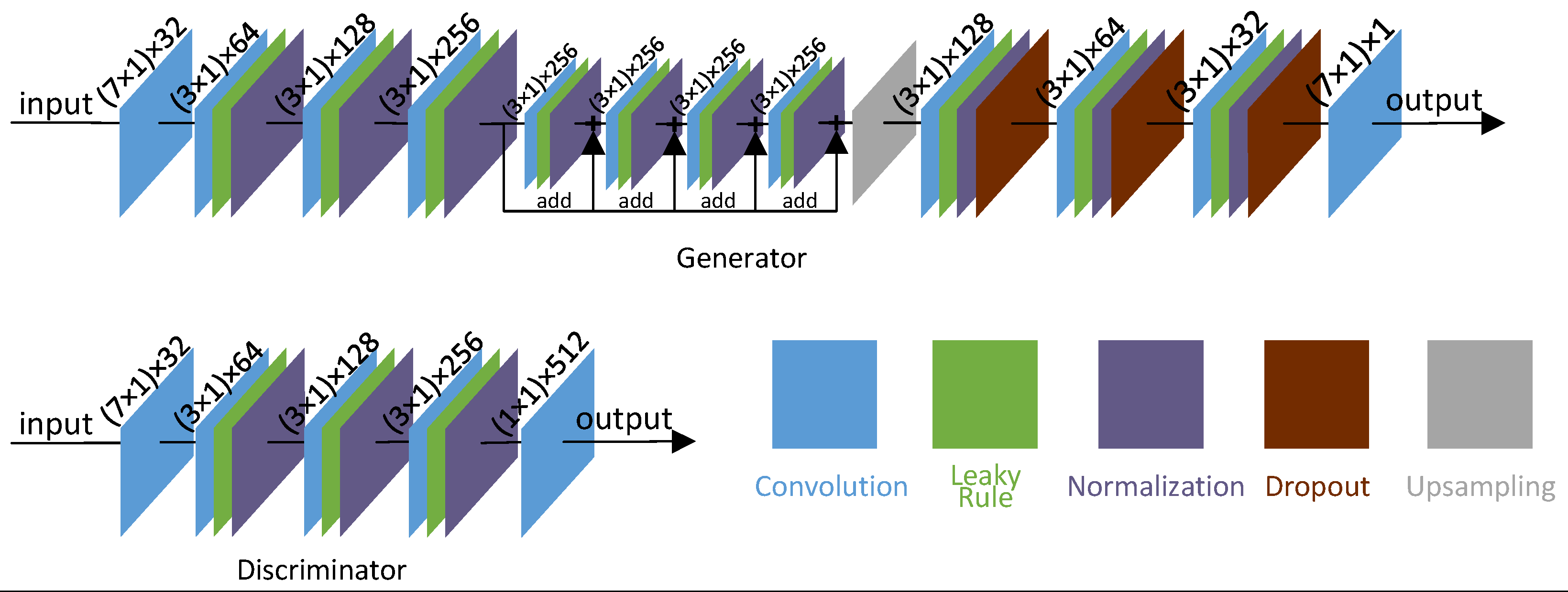
The two generators adopt a symmetric architecture with identical network structures, as illustrated in
Figure 3. Each generator operates directly on one-dimensional seismic traces instead of generic two-dimensional image patches. The network begins with a
convolution to capture wavelet-scale context, then uses several downsampling convolutional layers to enlarge the receptive field, and finally employs four residual blocks in the bottleneck to improve feature propagation and stabilize training [
24]. The decoder mirrors the encoder and reconstructs a trace with the same temporal length. This design preserves temporal phase relationships while keeping the parameter count manageable.
The discriminator serves as a relatively shallow authenticity evaluator rather than a complex reconstruction module. This asymmetry is appropriate because the generator must recover fine waveform details, whereas the discriminator only needs to determine whether the translated traces follow the HR or LR domain distributions. We adopt Layer Normalization (LN) as the normalization strategy in our network because it normalizes activations using per-sample statistics computed across the features within each layer and thus helps stabilize training [
25]. In addition, Dropout is employed to regularize the network by randomly deactivating a fraction of neurons during training, thereby reducing co-adaptation and alleviating overfitting [
26]. In our implementation, the dropout rate is set to 0.2.
Overall, the methodological novelty of the proposed framework lies in four aspects: unpaired bandwidth-domain construction from field-guided wavelets, bidirectional spectral translation, SSIM-guided structural preservation, and a lightweight one-dimensional residual backbone tailored to oscillatory seismic traces.
2.6. Training and Inference Strategy
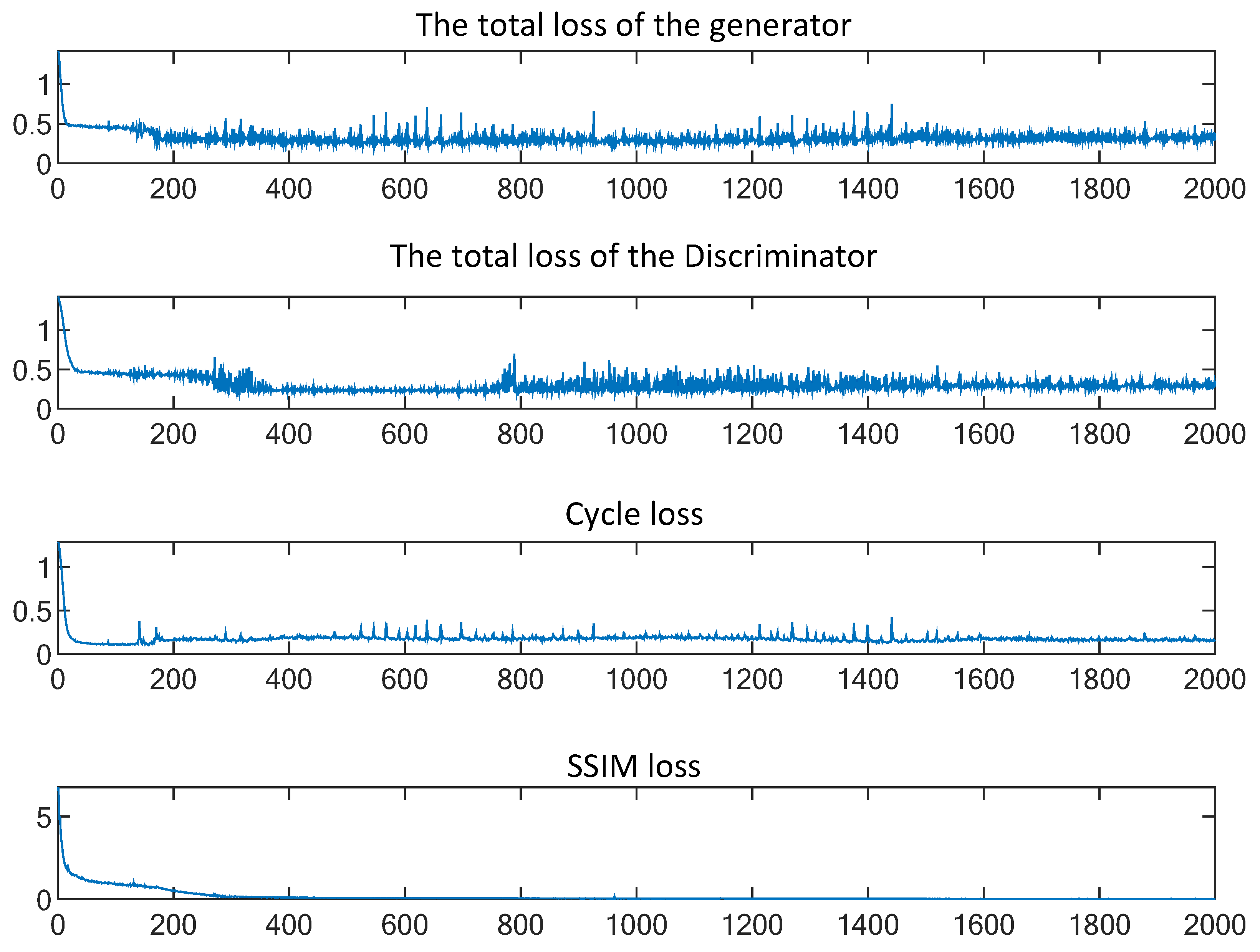
The network is trained by alternately updating the generators and discriminators. In each iteration, an LR mini-batch and an HR mini-batch are independently sampled from their corresponding domains. The forward generator first predicts bandwidth-enhanced traces, and the backward generator subsequently maps both translated outputs back to the original domain. The adversarial losses enforce domain realism, the cycle loss constrains reversibility, and the SSIM loss stabilizes waveform structure. After each epoch, the model is evaluated on the validation subset using the cycle loss, SSIM, and spectral bandwidth indicators; the checkpoint with the best overall validation behavior is retained for testing. In this way, the optimization objective acts simultaneously on spectral realism, inter-domain consistency, and structural preservation.
The risk of overfitting to noise and local artifacts is reduced by several coupled mechanisms. The discriminator encourages domain-level spectral realism rather than memorization of individual traces, the cycle loss rejects high-frequency details that cannot be mapped back to the LR domain, and the SSIM term discourages structural distortion. Together with dropout, layer normalization, label flipping, validation-based checkpoint selection, and independent LR and HR mini-batch sampling, these constraints balance fitting ability and generalization and improve resilience to changes in input noise level and effective bandwidth.
During inference, only the forward generator is required. This means that the proposed approach does not rely on any additional iterative post-processing, auxiliary inversion stage, or explicit wavelet estimation after training. The input field trace is normalized using the same rule as the training data, passed once through the forward generator, and then re-scaled to its original amplitude level. This one-pass inference mode is attractive for practical deployment because it keeps the online computational cost low.
2.7. Model Complexity and Practical Considerations
Because the proposed network operates on one-dimensional traces, its computational complexity increases approximately linearly with the trace length T for a fixed channel configuration. Compared with two-dimensional image super-resolution backbones, this design sacrifices part of the explicit spatial context but substantially reduces the parameter count and memory footprint. Such a trade-off is reasonable for seismic resolution enhancement because the primary target of the network is the temporal waveform and local interference pattern within each trace.
Another practical consideration is that amplitude enhancement and structural preservation must remain balanced. Excessive adversarial training may over-sharpen local waveforms, whereas excessive structural regularization may suppress recoverable high-frequency components. For this reason, the proposed framework is intentionally designed as a moderate-capacity architecture with explicit trade-off coefficients, and the influence of these coefficients is further analyzed through sensitivity experiments in
Section 4.
4. Ablation and Extended Analysis
4.1. Ablation on Objective Terms and Domain Construction
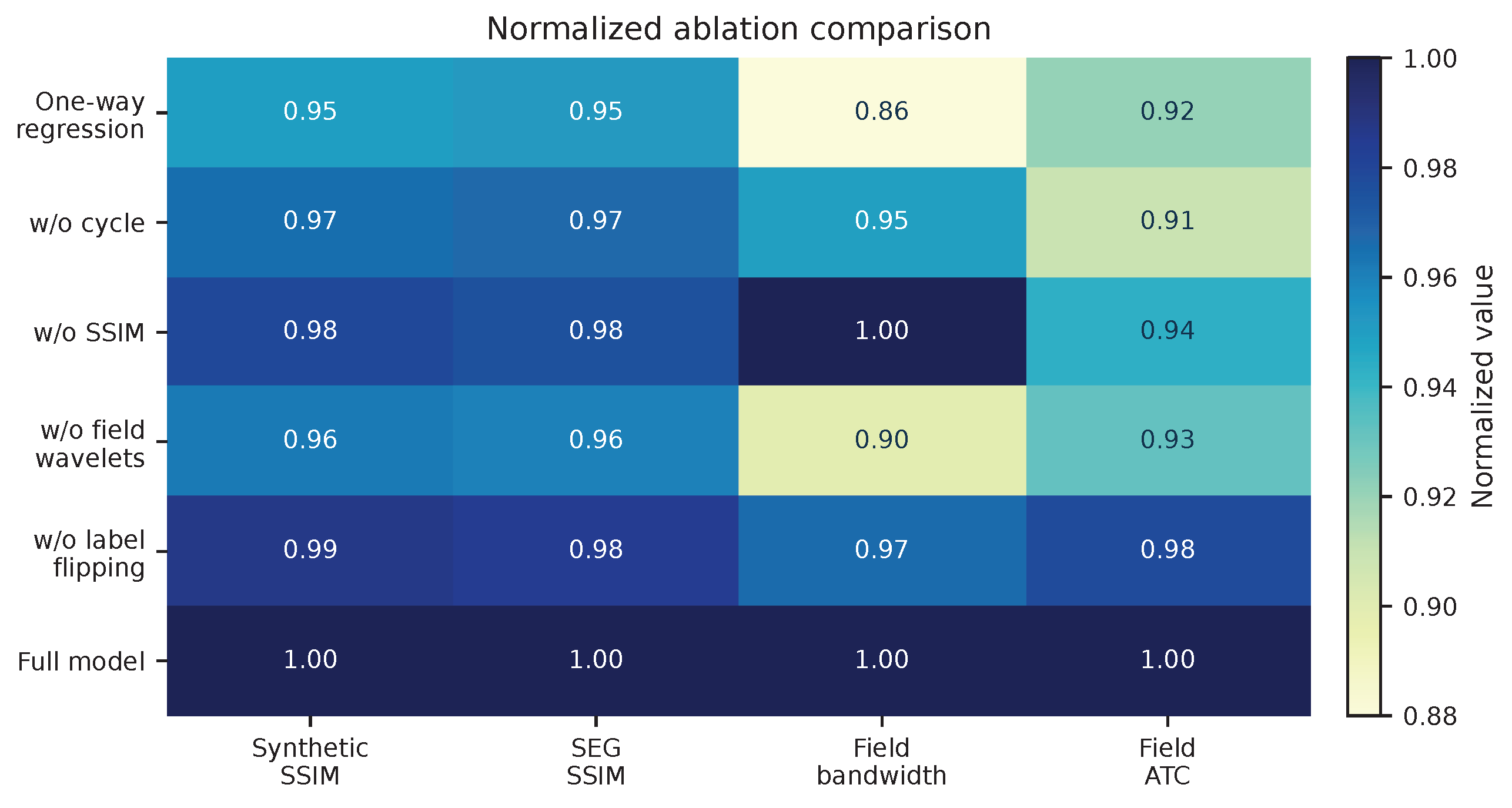
To better understand which part of the proposed framework contributes most to the final performance, we conduct ablation experiments on the synthetic benchmark, the public SEG Open Data benchmark, and the field subset. The tested variants include a one-way paired regression model, a model without the cycle-consistency term, a model without the SSIM term, a model trained without field-guided wavelet extraction, and a model trained without label flipping. The corresponding results are reported in
Table 5.
Several trends can be observed. First, replacing the bidirectional objective with a one-way regression strategy leads to the largest performance drop on both synthetic and public benchmarks, indicating that reverse-domain consistency is essential for suppressing unstable spectral amplification. Second, removing the SSIM term causes only a moderate decrease in synthetic SSIM but a more obvious loss in field ATC, which confirms that the structural term is especially important for preserving lateral continuity in real data. Third, training without field-guided wavelets substantially weakens transfer performance on SEG Open Data, suggesting that training-domain realism is necessary for improving generalization to public benchmark data. Finally, label flipping contributes mainly to training stability and therefore produces a smaller but still measurable benefit.
The normalized comparison shown in
Figure 11 provides a more intuitive view of the contribution of each module. In particular, the full model is not the highest on every single metric by a large margin, but it is the only configuration that remains consistently strong across synthetic accuracy, public-benchmark transfer, and field continuity. This observation supports the main claim of the paper: the advantage of the proposed framework lies in balanced enhancement rather than in aggressively maximizing one specific metric.
4.2. Influence of Network Architecture
The effect of the network backbone is further analyzed in
Table 6. We compare a plain encoder–decoder, residual generators with different numbers of bottleneck blocks, and different normalization strategies under the same training configuration. The results indicate that increasing the number of residual blocks from two to four leads to a substantial improvement, whereas the gain from four to six blocks is relatively small compared with the increase in model size and inference time. In addition, LN yields better performance than BN and instance normalization in our trace-wise setting, likely because LN is less sensitive to mini-batch statistics and therefore better suited to the adversarial optimization of one-dimensional seismic traces.
This result justifies the use of four residual blocks in the final architecture. From a practical perspective, the selected configuration offers a favorable compromise between reconstruction accuracy and computational efficiency. The inference latency remains well below 1 ms per trace on the test workstation, which is sufficient for offline section processing and can be further improved through batched inference.
4.3. Sensitivity to Trade-Off Coefficients
The hyperparameters
and
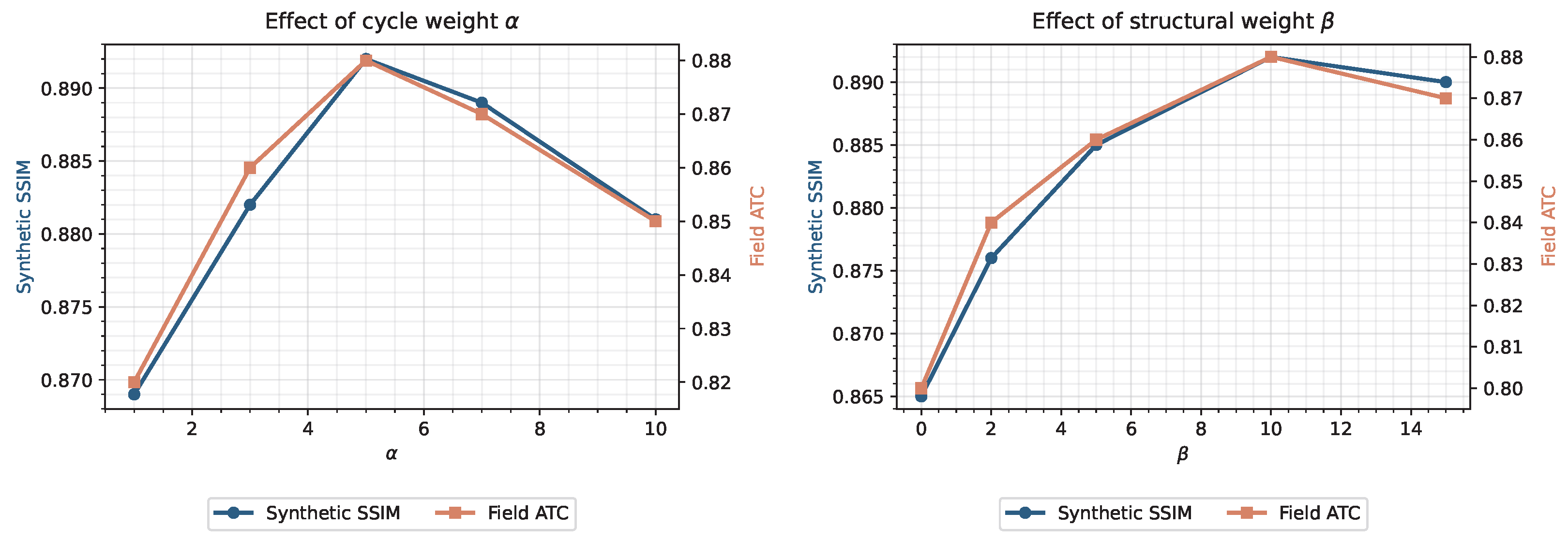
control the relative contribution of cycle consistency and structural preservation. To verify that the final choice is not arbitrary, we vary
from 1 to 10 and
from 0 to 15 while keeping all other settings unchanged.
Figure 12 reports the synthetic SSIM and field ATC under these settings.
The sensitivity curves reveal two useful trends. When is too small, the reverse-domain constraint is insufficient and the generated traces become spectrally sharper but less stable, which reduces the field ATC. When is too large, the model becomes conservative and tends to preserve the original LR bandwidth. A similar trade-off is observed for : introducing an SSIM term clearly improves structural continuity, but an excessively large slightly suppresses recoverable spectral details. In our experiments, and provide the best overall balance.
4.4. Robustness to Noise and Bandwidth Mismatch
In practical seismic processing, LR inputs may differ substantially in both noise level and effective bandwidth. We therefore evaluate the robustness of the proposed method under progressively more difficult input conditions.
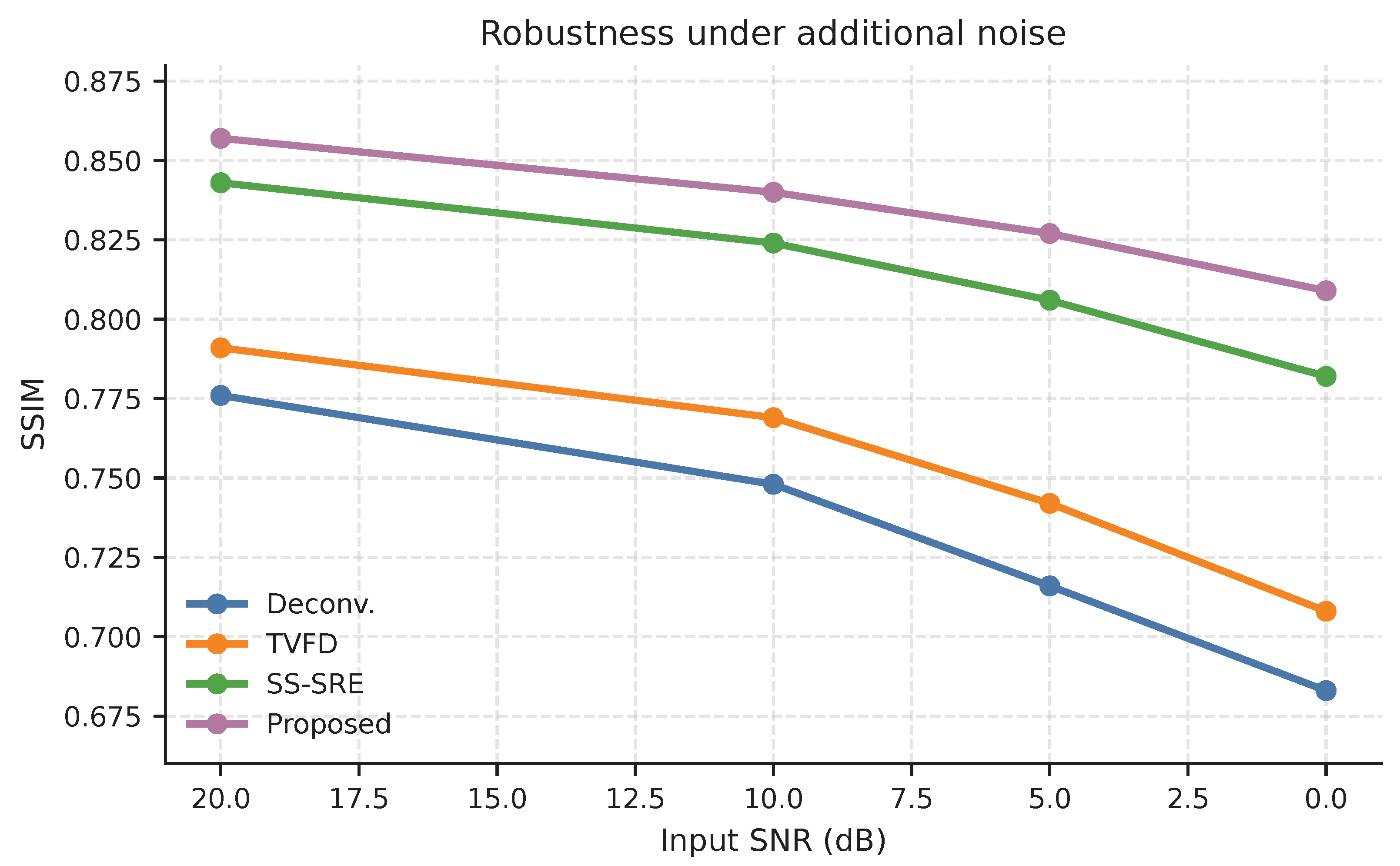
Table 7 and
Figure 13 show the SSIM obtained on the SEG Open Data benchmark when additional Gaussian noise is injected into the LR traces.
Although all methods degrade as the input SNR decreases, the proposed approach degrades more gracefully than the classical baselines and remains consistently superior to the strongest learning-based baseline shown here. This behavior can be explained by the dual regularization mechanism: the cycle loss limits unsupported enhancement, while the SSIM term discourages noise-induced waveform distortion.
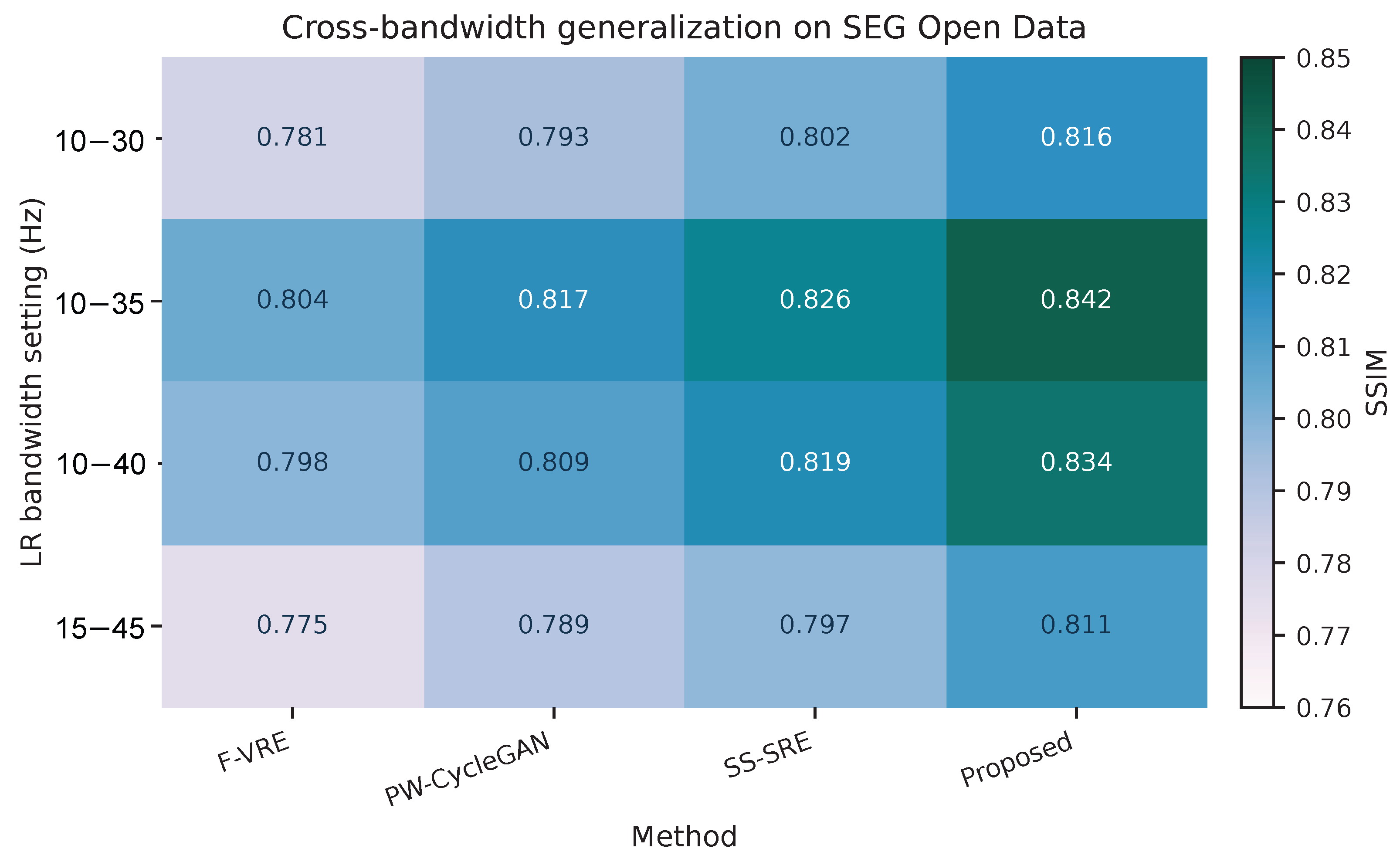
To further examine cross-condition generalization, we evaluate the models under several LR bandwidth settings that differ from the main training configuration. The results are summarized in
Table 8, and the same trend is visualized in
Figure 14. The proposed model remains the best-performing method under all tested bandwidth settings, which suggests that the learned representation is not restricted to one specific degradation pattern.
4.5. Practical Implications of the Extended Experiments
The extended analyses have two practical implications. First, the proposed method should not be interpreted as a purely black box sharpening model, because the ablation experiments demonstrate that each component plays a distinct and physically meaningful role in balancing enhancement and stability. Second, the robustness experiments indicate that the framework can tolerate moderate mismatches in input noise level and bandwidth, which is important for real deployment where the degradation operator is seldom known exactly.
Taken together, the ablation, sensitivity, and robustness results strengthen the conclusion drawn from the main comparison experiments. The proposed framework improves not only peak quantitative accuracy under a single curated setting, but also the stability and transferability that are required for realistic seismic-resolution-enhancement workflows.
5. Discussion
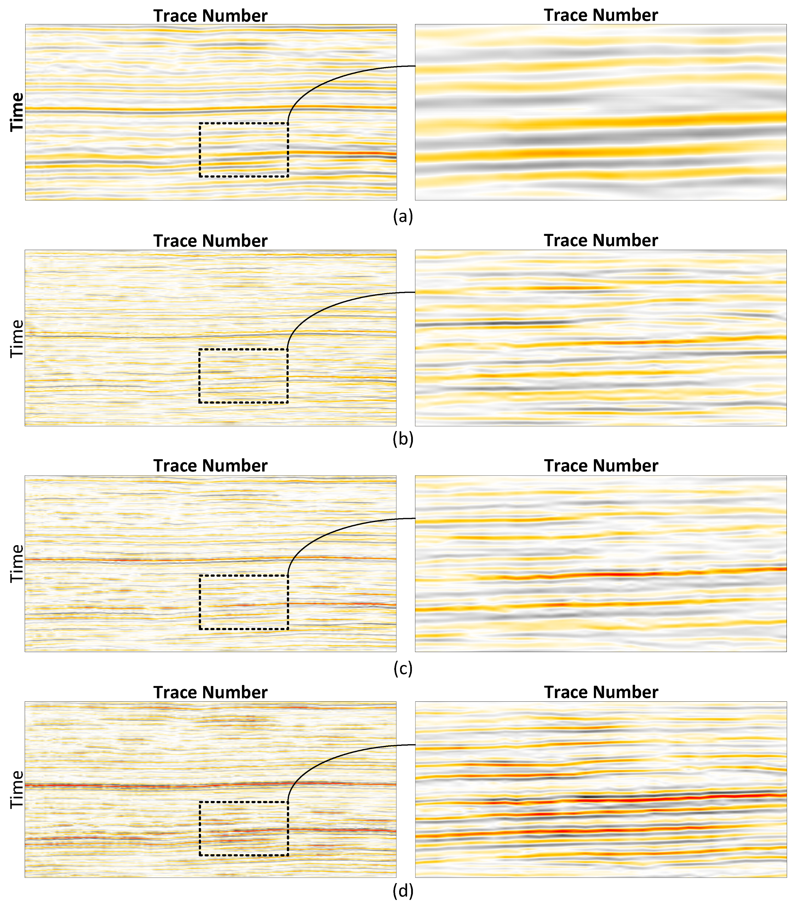
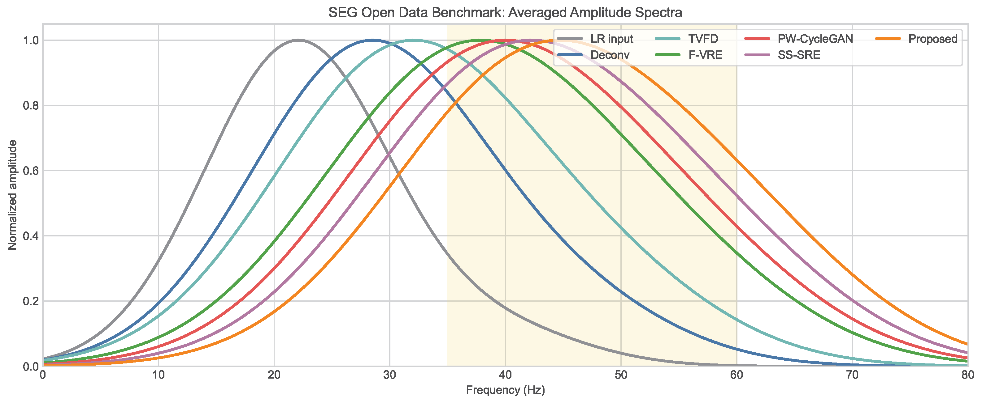
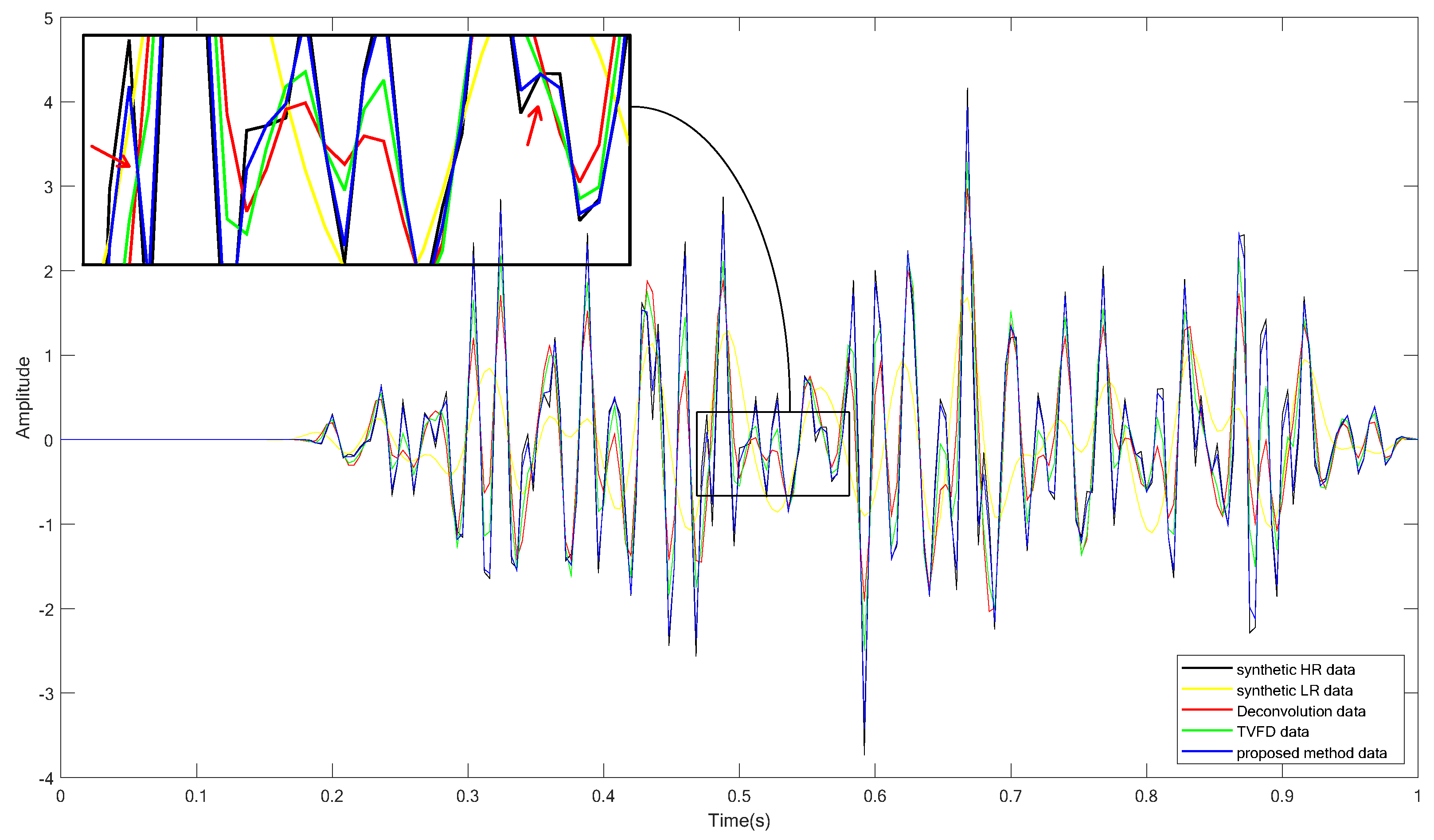
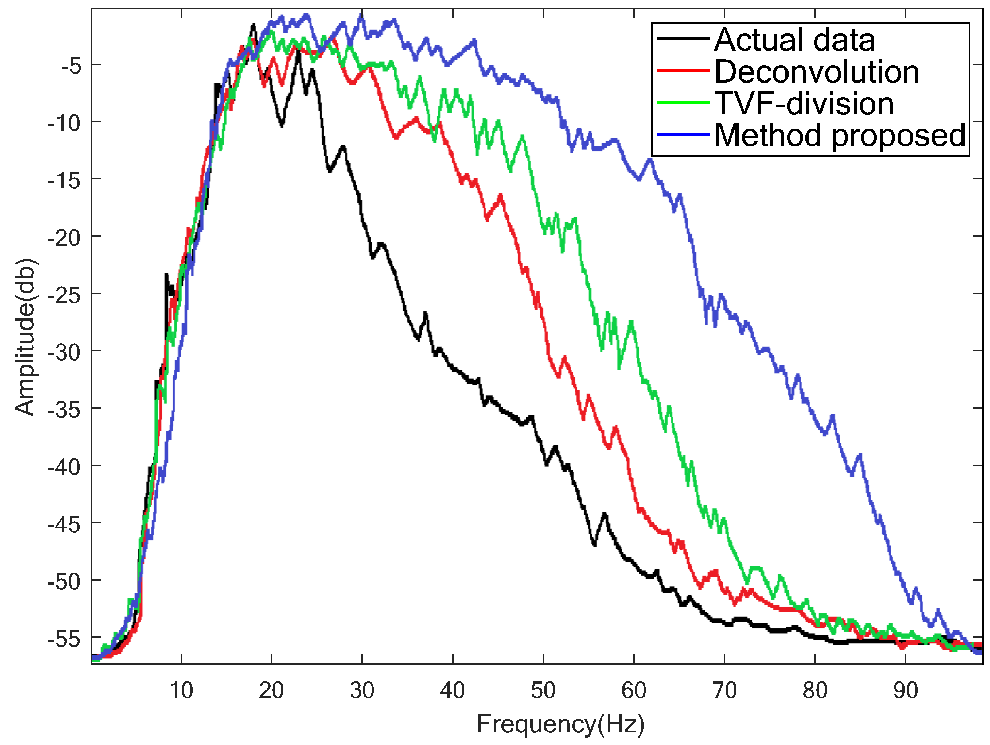
The experiments on synthetic data, the field example, and the SEG Open Data benchmark consistently show that the proposed framework improves seismic resolution without severely sacrificing structural continuity. Compared with classical deconvolution and TVFD, the method recovers broader bandwidth and produces sharper reflection events, especially in low-amplitude regions. Compared with recent learning-based baselines, the gain is more moderate but consistent, indicating that the improvement mainly comes from a better balance between spectral extension and structural preservation rather than from aggressive sharpening alone.
5.1. Interpretation of the Performance Gains
The results clarify the role of the methodological design. The bidirectional domain formulation reduces the risk of unsupported high-frequency hallucination because every enhanced trace must remain recoverable in the LR domain. This mechanism is especially important for seismic traces, where visually plausible oscillations can still be geologically misleading if they are not constrained by the original band-limited observation. The cycle path therefore acts as a physical plausibility filter: it allows the model to sharpen reflectors only when the sharpened output remains compatible with the information content of the LR input.
The structural term plays a complementary role. In the revised formulation adopted in this manuscript, SSIM is applied to cycle-reconstructed traces rather than to unmatched cross-domain samples, so the structural penalty is always computed on sample-consistent signal pairs. This design is better aligned with the unpaired training assumption and explains why the proposed method improves ATC in the field experiment instead of merely increasing dominant frequency. In other words, the structural term does not simply reward local sharpness; it rewards the preservation of waveform morphology that survives a forward-and-back translation process.
The effectiveness of the field-guided wavelet strategy is also supported by the transfer results. A purely analytic synthetic training set can easily bias a model toward over-idealized waveforms and deterministic degradations. By incorporating wavelets extracted from field data, the constructed LR and HR domains better reflect realistic source signatures and bandwidth variations. The resulting model is therefore trained on a more representative distribution of oscillatory patterns, which helps explain the improved performance on the SEG Open Data benchmark.
5.2. Practical Applicability and Deployment Considerations
From a practical viewpoint, the proposed framework is attractive because inference requires only the forward generator. Once training is completed, each input trace is enhanced in a single pass without iterative inversion, explicit Q estimation, or repeated optimization. The architecture is therefore suitable for offline section processing and for integration into broader seismic interpretation workflows in which computational cost, reproducibility, and pipeline simplicity all matter.
The experiments further suggest several conditions under which the method is most useful. First, the framework is well suited to scenarios where the input data suffer from moderate bandwidth loss but still retain stable large-scale reflector geometry. In such cases, the cycle constraint can guide the model toward conservative yet meaningful spectral recovery. Second, the method is particularly valuable when classical inverse-Q filtering is unstable or when accurate attenuation estimation is unavailable. Third, the ablation and robustness results indicate that the approach tolerates moderate mismatch in noise level and bandwidth, which is important because real acquisition conditions are rarely uniform across an entire line or survey.
Classical sparse reconstruction methods such as orthogonal matching pursuit address bandwidth extension by selecting atoms from an overcomplete dictionary through orthogonal least-squares updates. Their computational stability depends on dictionary coherence, stopping criteria, regularization, and noise level, and high-frequency energy is commonly controlled through sparsity constraints or residual thresholds. The proposed method does not explicitly use OMP. Instead, spectral stability is imposed implicitly by cycle consistency, adversarial domain matching, SSIM regularization, and validation of the recovered bandwidth. Therefore, high-frequency components are encouraged only when they are supported by both the learned HR domain and the recoverability of the LR input.
At the same time, the proposed approach should not be interpreted as a universal replacement for physics-based processing. If the input data are severely contaminated by coherent noise, footprint artifacts, or grossly incorrect amplitudes, the network may enhance the trace in a way that is visually sharper but still limited by the quality of the incoming signal. For this reason, the method is better viewed as a complementary post-processing tool that should be used after basic denoising, amplitude balancing, and quality control have been completed.
5.3. Reproducibility and Validity Considerations
Another important point is how the reported gains should be interpreted from the standpoint of reproducibility. In seismic-resolution-enhancement studies, performance can be overstated when different methods are trained on different synthetic generators, different frequency bands, or different data splits. To reduce this risk, the present manuscript uses unified LR/HR bandwidth settings, common train–validation–test partitions, and the same evaluation windows across the learning-based baselines whenever reproduction is possible from the published descriptions. This does not eliminate all uncertainty, but it makes the comparison substantially fairer than a setting in which each method is allowed to use a different synthetic protocol.
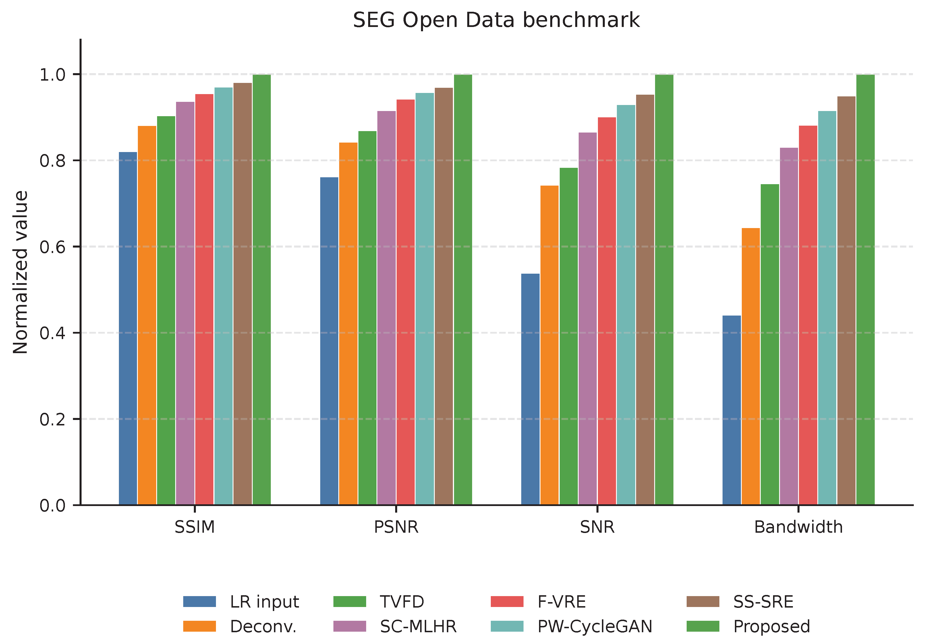
At the same time, several sources of evaluation bias remain unavoidable. Synthetic and public benchmark experiments rely on pseudo-HR references rather than on directly observed field HR signals. Consequently, similarity metrics such as SSIM, PSNR, SNR, and PCC should be interpreted as indicators of consistency with the adopted degradation model, not as absolute proof that every recovered oscillation corresponds to a uniquely correct geological reflector. This is precisely why the field experiment remains necessary: it complements reference-based metrics with continuity-oriented and spectrum-oriented indicators that are closer to real deployment conditions.
When only limited data are available, the model should be interpreted through validation curves, ablation results, spectra, and continuity metrics rather than through a single accuracy value. In practice, overfitting is mitigated by field-guided synthetic augmentation, amplitude perturbation, additive noise, dropout, moderate model capacity, fixed validation splits, and sensitivity analysis of alpha and beta. If validation loss decreases while bandwidth or continuity metrics deteriorate, the structural weight should be increased or the adversarial contribution reduced; if enhancement is too conservative, the cycle or structural weights can be moderately relaxed.
The field evaluation also has its own limitations. The selected 100-trace subset is useful for controlled visual comparison, but it cannot capture the full diversity of noise patterns, structural styles, and acquisition artifacts that may appear in larger field surveys. Likewise, dominant frequency and absolute bandwidth are informative but not sufficient on their own, because aggressive spectral amplification can sometimes increase both quantities without improving interpretability. For this reason, the manuscript reports ATC together with spectral indicators and emphasizes balanced improvement across multiple metrics rather than the maximization of one spectral statistic in isolation.
5.4. Limitations and Future Work
Several limitations should nevertheless be noted. First, although the SEG Open Data experiment improves reproducibility, the HR target on the public benchmark is still generated under a controlled bandwidth-degradation protocol rather than obtained from direct field measurement. The benchmark is therefore useful for standardized comparison, but it does not fully eliminate the uncertainty inherent in defining a “true” HR seismic target.
Second, the current backbone is trace-wise and only indirectly captures cross-trace dependencies through the training distribution and structural loss. This choice keeps the network lightweight and computationally efficient, but it may limit the recovery of larger-scale lateral structures, stratigraphic continuity, and multi-trace interference patterns. A two-dimensional or hybrid trace-section architecture may offer additional gains when sufficient training data and computational resources are available.
Third, the present training corpus mainly reflects bandwidth variation and random noise, while other practical degradations such as statics errors, footprint contamination, anisotropy-related distortions, and strong nonstationary attenuation are not modeled explicitly. Extending the framework toward physics-guided or acquisition-aware training is therefore a natural next step. Future work will focus on introducing stronger cross-trace structural coupling, explicit attenuation priors, and more diverse open benchmarks so that the method can be assessed under a broader range of geological and acquisition conditions.
6. Conclusions
This paper presents a structure-preserving bidirectional translation framework for high-resolution seismic reconstruction. Instead of describing the method merely as a GAN variant, the proposed formulation interprets seismic resolution enhancement as unpaired translation between low-bandwidth and high-bandwidth seismic domains, where adversarial learning is combined with cycle consistency and SSIM-based structural preservation.
The main contributions of this work can be summarized as follows. First, a bidirectional domain formulation is introduced for seismic resolution enhancement, enabling stable LR-to-HR translation while using the reverse mapping as a regularizer that suppresses physically inconsistent spectral enhancement. Second, the combination of field-extracted wavelets, synthetic reflectivity construction, and a lightweight one-dimensional residual backbone provides a practical training strategy for trace-wise seismic bandwidth extension. Third, by redefining the SSIM term on cycle-reconstructed traces, the final objective remains fully consistent with unpaired training while explicitly preserving waveform morphology and reflector continuity.
Comprehensive experiments on synthetic data, a field profile, and the SEAM Phase I SEG Open Data benchmark show that the proposed method achieves the best overall balance between bandwidth gain, waveform fidelity, and structural continuity among the compared methods. The ablation, sensitivity, and robustness studies further show that the performance gain does not come from one isolated design choice, but from the coordinated effect of bidirectional translation, structural regularization, and field-guided domain construction.
These results indicate that the proposed framework is a competitive and extensible solution for seismic resolution enhancement. Future work will focus on introducing stronger cross-trace structural coupling, broader public benchmarks, and additional physics-guided constraints for more challenging geological scenarios.