Improvement of PC-SAFT-Based Asphaltene Prediction Model and Simulation of Phase Behavior Under Multiple Operating Conditions

Abstract

This study, based on phase equilibrium theory, uses reservoir crude oil systems as the research object and adopts the Perturbed Chain-Statistical Associating Fluid Theory (PC-SAFT) equation of state. By combining the Panuganti characterization method with the three-phase Rachford–Rice algorithm, an integrated RRPC-SAFT engineering workflow is established, which effectively addresses the drawbacks of traditional PC-SAFT models, including low computational efficiency and poor convergence under extreme working conditions. On this basis, systematic performance comparisons are conducted between the RRPC-SAFT workflow and classical cubic equations of state (PR and SRK). Furthermore, the asphaltene phase behavior under gas injection development conditions is simulated, and the quantitative effects of the four SARA fractions on the critical precipitation conditions and precipitation intensity of asphaltenes are determined, clarifying the evolution rules and main controlling factors of asphaltene phase instability under various development scenarios. The research results reveal that the average relative errors of bubble point pressure and asphaltene onset precipitation pressure (AOP) for the three crude oil samples are all less than or equal to 5%. Compared with the PR and SRK models, the average prediction errors are reduced by 1.27% and 2.01%, respectively. Gas injection simulation results demonstrate that nitrogen poses the highest risk of triggering asphaltene precipitation under equimolar injection, with the asphaltene onset precipitation pressure increasing up to 114.94%. Single-factor analysis of SARA fractions verifies that saturates and asphaltenes aggravate precipitation, while aromatics and resins suppress asphaltene destabilization. In terms of computational efficiency, the computational speed of the RRPC-SAFT algorithm is four times higher than that of the traditional Gibbs free energy minimization algorithm. This model can be applied to calculate the thermodynamic critical equilibrium conditions of asphaltene precipitation, providing a thermodynamic basis for early screening of asphaltene deposition risks, optimization of gas injection schemes, and design of deposition prevention and control technologies.

1. Introduction

Asphaltenes are the components with the highest relative molecular weight and strongest polarity in crude oil, characterized by high aromaticity, strong self-association, and thermodynamic instability. They are generally defined as a class of compounds that are insoluble in n-heptane but soluble in aromatic solvents [1,2]. With global oil and gas development extending to deep, low-permeability, and heavy oil reservoirs, and the large-scale promotion of enhanced oil recovery technologies such as CO₂ flooding, the problems of reservoir damage and wellbore blockage caused by asphaltene deposition have become increasingly prominent and have emerged as one of the core challenges restricting the efficient development of oil and gas fields. This problem is particularly prominent in low-permeability reservoirs such as shale oil and tight oil, where surface adsorption and pore throat blockage induced by asphaltenes lead to a remarkable production decline, emerging as one of the key bottlenecks, restricting the efficient development of oil and gas fields and the industrial implementation of carbon sequestration [3].

Regarding asphaltene deposition prediction, three core thermodynamic systems have been established: solubility models, colloid models, and equation of state models [4,5]. Among them, the solubility model is constructed based on the principle of similar miscibility, with easy-to-obtain parameters but ignores molecular association, resulting in a limited application scope [6,7,8]; the colloid model can explain the dispersion and stabilization effect of resins on asphaltenes, but its core parameters mostly rely on experimental fitting, leading to weak generalization ability; the equation of state model, by virtue of its accurate description of intermolecular interactions, can simultaneously describe vapor–liquid, liquid–liquid, and vapor–liquid–solid multiphase equilibrium behaviors, and has become the mainstream research direction in this field. However, traditional PC-SAFT models have problems such as low computational efficiency and poor convergence under extreme working conditions, and existing studies have insufficient quantification of the deposition regulation laws of the endogenous SARA four components in crude oil, making it difficult to meet the needs of on-site engineering applications [9,10].

Early studies on asphaltene phase behavior were mainly carried out based on classical cubic equations of state. In 2003, Vafaie et al. [11] introduced an association term into the PR equation to compensate for the insufficient description of asphaltene polarity by traditional cubic equations, but only used a simple empirical relationship to calculate the deviation coefficient term, lacking support from correlations with clear physical meaning. In 2006, Sabbagh et al. [12] used the group contribution method to adjust the parameters of the PR equation of state and divided asphaltenes into three sub-components to simulate the precipitation behavior of n-alkane-diluted systems, which improved the prediction accuracy of heavy oil systems to some extent; however, this approach still did not overcome the inherent limitations of the mean field theory.

With the development of statistical thermodynamics, a series of equations of state based on the Statistical Associating Fluid Theory (SAFT) have gradually become the core of research. These equations describe the repulsion, attraction, and association of chain molecules from the molecular level, and their ability to describe the phase equilibrium of asymmetric macromolecular systems is significantly better than that of classical cubic equations. In 2003, Ting et al. [13] first applied the SAFT equation to asphaltene phase behavior simulation. In the same year, Ting [14] further proposed that asphaltene precipitation is a reversible thermodynamic process, that the precipitated phase is a pseudo-component liquid phase, and that only van der Waals dispersion forces dominate molecular association and aggregation, thereby introducing the PC-SAFT equation of state into asphaltene precipitation calculations for the first time. Subsequently, Wu et al. [15,16] regarded the remaining components of crude oil as a continuous medium and described the dispersion force between asphaltenes and resins through the Hamaker constant [17]. The model’s calculation error for asphaltene precipitation pressure was less than 7%, but it could not be independently applied to the phase behavior simulation of gas-bearing crude oil systems. From 2004 to 2007, Gonzalez et al. [18,19] proposed the Variable Range Statistical Associating Fluid Theory (SAFT-VR) and used the SARA four-component analysis method to characterize degassed oil, but the model only considered the dispersion force between asphaltene molecules and ignored the interaction between polar components. In 2010, Li et al. [20] introduced the Cubic-Plus-Association (CPA) equation of state into asphaltene deposition research, which can simultaneously describe the self-association of asphaltenes and the polar interactions with aromatics and resins [21], and further improved the characterization method of crude oil systems to enhance model accuracy [22]. However, the model parameter calibration still relies on a large number of experimental fittings, resulting in a limited generalization ability.

The PC-SAFT equation has gradually become the standard model for asphaltene phase behavior simulation due to the clear physical meaning of its parameters and its strong adaptability to heavy hydrocarbon systems. In 2012, Panuganti et al. [23] proposed a standardized characterization method for crude oil systems based on PC-SAFT, dividing crude oil into 10 pseudo-components and using the aromaticity parameter to describe the structural characteristics of aromatics + resins (A + R). In 2013, they further optimized the characterization method, simplifying crude oil into two pseudo-component systems: a flash vapor phase and a tank oil phase, and only needed to adjust the average molecular weight of asphaltenes to match the experimental data of asphaltene onset precipitation pressure (AOP) [24]. In 2016, Tavakkoli et al. [25] divided asphaltenes into four sub-components and fitted the precipitation experimental data through a distribution function, improving the matching effect of asphaltene precipitation behavior in lighter n-alkane systems. In 2022, Ghasemi et al. [26] carried out field crude oil asphaltene precipitation studies under high-temperature and high-pressure conditions, and proposed a multi-parameter simultaneous optimization method to replace the traditional step-by-step parameter adjustment strategy, which reduced the prediction error of heavy oil systems by 5% to 12% and expanded the applicability of the model under extremely high-temperature and high-pressure working conditions.

To clearly distinguish the technical routes, research content, and research focus of previous studies and the present work, the investigations by Panuganti, Parsaei, Ghasemi, and this paper are compared in

Table 1. Comparison of Research Approaches by Panuganti, Parsaei, Ghasemi, and the present work.

Research Object	Crude Oil Characterization	Solution Algorithm	Main Research Content
Panuganti	Stepwise standardized characterization	Traditional Gibbs algorithm	Basic SARA fraction analysis
Parsaei	Simplified characterization	Three-phase RR algorithm	Phase diagram simulation
Ghasemi	Classical characterization	Traditional algorithm	Gas injection simulation
This work	Stepwise standardized characterization	Fast RR algorithm	Gas injection schemes coupled with quantitative SARA fraction analysis

.

This work excludes investigations on molecular aggregation kinetics, interfacial adsorption, and actual asphaltene deposition and plugging processes in reservoirs and pipelines. The paper focuses on the thermodynamic phase equilibrium of asphaltenes to establish a fast-solving RRPC-SAFT model, quantify the critical precipitation thresholds and evolutionary patterns of asphaltenes under various operating conditions, and provide a thermodynamic basis for subsequent deposition kinetic simulations and field deposition risk control. Three typical domestic continental crude oil samples, namely, a high gas–oil ratio (GOR) black oil, high CO₂-content crude oil, and a light crude oil with a low asphaltene concentration, are adopted for model validation, covering common gas injection development scenarios. The RRPC-SAFT workflow is built upon the PC-SAFT molecular thermodynamic framework and employs a multi-pseudo-component splitting characterization strategy, which theoretically supports the characterization of diverse fluids, including heavy oil, high-wax crude oil, and ultra-high GOR crude oil. However, restricted by the availability of experimental measurement data, experimental calibrations for heavy oil and coupled wax–asphaltene systems are not implemented in this study. Verification of such extreme fluid systems will be prioritized in future research.

2. PC-SAFT Equation of State

Gross et al. [27] proposed the Perturbed Chain-Statistical Associating Fluid Theory (PC-SAFT) based on the second-order perturbation theory proposed by Barker et al. [28]. It has the ability to handle the thermodynamic behavior and phase equilibrium of systems containing heavy hydrocarbons and systems with large molecular weight differences (such as asphaltene and polymer systems). Traditional SAFT models only consider the chain shape of molecules in the hard-chain term (repulsion term) of the equation of state, while the PC-SAFT model also considers the chain length dependence of dispersion interactions. The PC-SAFT equation of state improves the deficiency of SAFT models in describing the dispersion term by extending it to the hard-chain reference system and adjusting the model constants. This model is superior to the cubic equations of state of classical petroleum models in describing the phase behavior of mixtures with large molecular size differences and liquid compressibility. The contribution of the dispersion term compensates for the description of molecular non-sphericity and narrows the gap between statistical mechanics models and classical petroleum engineering models. The PC-SAFT equation is the most widely used in the SAFT series of equations and is regarded as the standard equation of state for describing complex macromolecular systems [29].

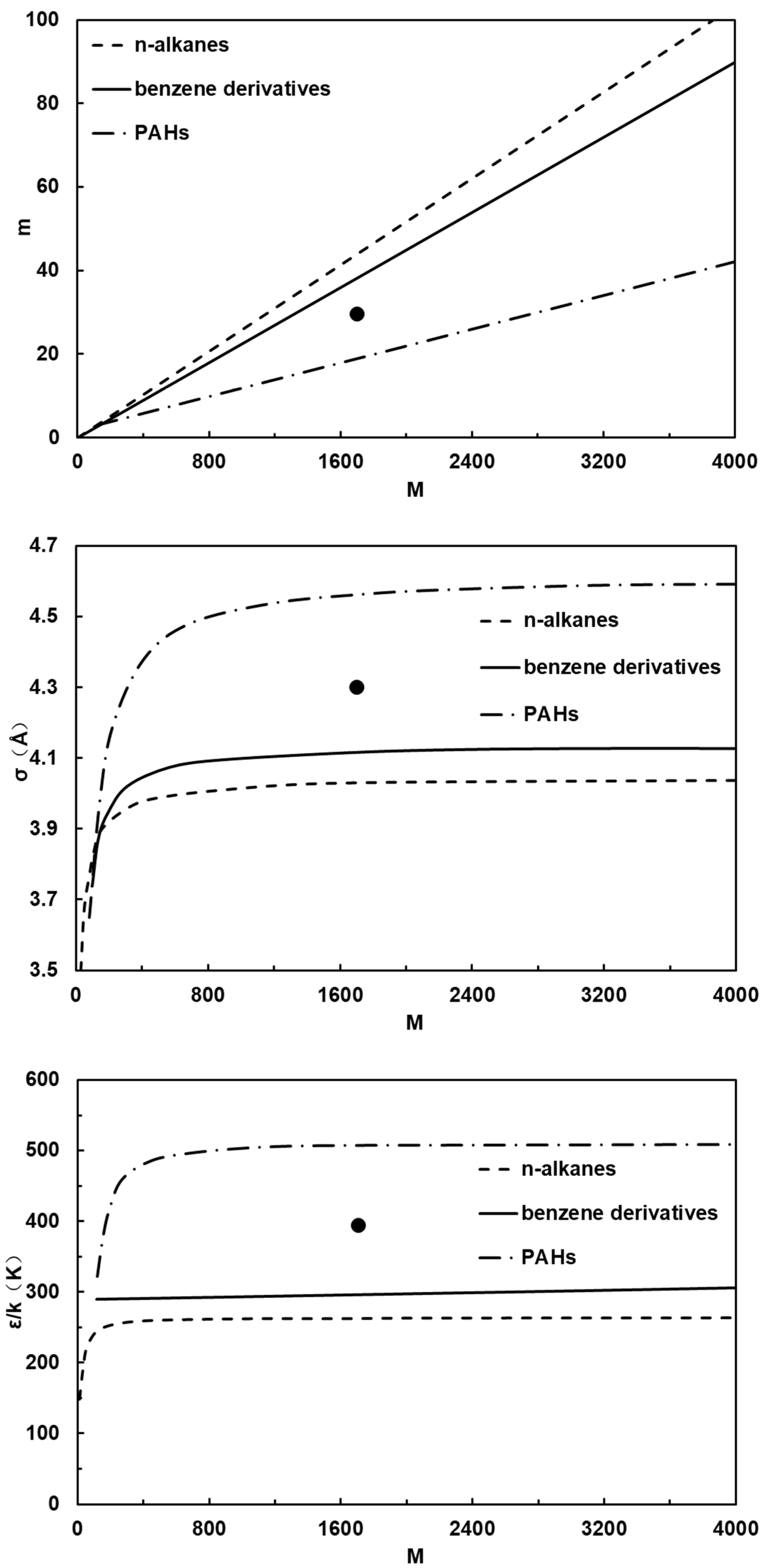
For non-associating fluids, the PC-SAFT model uses mole fraction x_i, segment number m_i, segment diameter σ_i, and segment interaction energy ε_i/k to solve parameters such as the residual Helmholtz free energy and the deviation factor. These parameters are usually obtained by fitting the experimental vapor pressure and liquid density of pure components. The PC-SAFT equation of state describes the fluid behavior as a function of temperature, volume, and mole number using the Helmholtz free energy, and thermodynamic properties can be obtained by differentiating the independent variables in the Helmholtz free energy expression.

In the macroscopic liquid–liquid equilibrium process of asphaltene precipitation from crude oil, dispersion forces dominate the overall intermolecular interactions of the system. Polar association mainly affects the internal structure of microscopic asphaltene aggregates and does not change the macroscopic thermodynamic characteristics of the system, such as the phase equilibrium boundary and asphaltene onset pressure (AOP); this conclusion has been verified by numerous asphaltene PVT experiments and simulation studies [30,31,32]. In addition, the association parameters of crude oil systems are difficult to obtain, and their introduction will significantly increase the number of parameters to be solved in the model and raise the difficulty of parameter calibration. For conventional oilfield crude oils, after disabling the association term, the prediction accuracy of the model for bubble point pressure and asphaltene precipitation pressure can still meet the requirements of engineering design, which is also a generally accepted simplification scheme in the current field of PC-SAFT asphaltene modeling [23,24]. Therefore, the SAFT association term is not considered, and the Helmholtz free energy consists of contributions from both the hard-chain reference term and the dispersion perturbation term:

$${\tilde{a}}^{res}={\tilde{a}}^{hc}+{\tilde{a}}^{disp}$$

(1)

where ${\tilde{a}}^{res}$ is the residual Helmholtz free energy; ${\tilde{a}}^{hc}$ is the Helmholtz free energy of the hard-chain term; ${\tilde{a}}^{disp}$ is the Helmholtz free energy of the dispersion term.

Similar to the virial equation, the PC-SAFT model also defines the compressibility factor as the sum of the ideal gas compressibility factor 1, the hard-chain contribution, and the perturbation term:

$$Z=1+Z^{hc}+Z^{disp}$$

(2)

where Z^hc is the compressibility factor of the hard-chain reference term (repulsion); Z^disp is the compressibility factor of the dispersion perturbation (attraction) term.

The expression for the average segment number $\overline{m}$ is:

$$\overline{m}={\displaystyle \sum _{i=1}^N{x}_i}{m}_i$$

(3)

The radial distribution function $g_{ij}^{hs}$ describes the relative spacing of molecules in the mixture. For segments of components i and j, the radial distribution function is:

$$g_{ij}^{hs}={\displaystyle \frac{1}{1-{\zeta }_3}}+{\displaystyle \frac{d_i d_j}{d_i+d_j}}{\displaystyle \frac{3{\zeta }_2}{\left(1-{\zeta }_3\right)}}+{\left({\displaystyle \frac{d_i d_j}{d_i+d_j}}\right)}^2{\displaystyle \frac{2{\zeta }_2^2}{{\left(1-{\zeta }_3\right)}^3}}$$

(4)

The coefficient ζ_n is a size parameter, and its expression is:

$${\zeta }_n={\displaystyle \frac{\pi }{6}}\rho {\displaystyle \sum _{i=1}^N{x}_i}{m}_i{d}_i^n$$

(5)

where ζ₀, ζ₁, ζ₂, ζ₃ are the parameters related to system properties, determined by molecular structure and intermolecular forces.

The total molecular density ρ is:

$$\rho ={\displaystyle \frac{6\eta }{\pi {\displaystyle \sum _{i=1}^N{x}_i}{m}_i{d}_i^3}}$$

(6)

where η is the packing fraction, also known as reduced density, equal to ζ₃.

The temperature-dependent effective segment diameter d_i is:

$$d_i={\sigma }_i\left[1-0.12\exp \left(-{\displaystyle \frac{3{\epsilon }_i}{kT}}\right)\right]$$

(7)

where k is the Boltzmann constant; T is the temperature.

The mixing parameters are obtained from the traditional Berthelot–Lorentz mixing rules:

$${\epsilon }_{ij}=\sqrt{{\epsilon }_i{\epsilon }_j}\left(1-k_{ij}\right)$$

(8)

$${\sigma }_{ij}={\displaystyle \frac{1}{2}}\left({\sigma }_i+{\sigma }_j\right)$$

(9)

where k_ij is a binary interaction parameter.

The calculation of the fugacity coefficient is particularly important, as it is used in the calculation of Gibbs free energy, fugacity, and equilibrium constants, which are used to determine the equilibrium state of the mixture. The fugacity coefficient φ_k(T, P) is related to the residual chemical potential ${\mu }_k^{res}$ and is calculated by the following formula:

$$\ln {\phi }_k={\displaystyle \frac{{\mu }_k^{res}(T,\nu )}{kT}}-\ln Z$$

(10)

The residual chemical potential refers to the difference in chemical potential between a real fluid and an ideal gas at the same temperature and pressure, reflecting the contribution of intermolecular interactions in the real fluid to the chemical potential, which can be derived from the following formula:

$${\displaystyle \frac{{\mu }_k^{res}(T,v)}{kT}}={\tilde{a}}^{\mathrm{res}}+(Z-1)+{\left({\displaystyle \frac{\partial {\tilde{a}}^{res}}{\partial x_k}}\right)}_{T,v,x_{i\ne k}}-{\displaystyle \sum _{j=1}^N\left[x_j{\left(\frac{\partial {\tilde{a}}^{res}}{\partial x_j}\right)}_{T,v,x_{i\ne j}}\right]}$$

(11)

The exclusion of the association term in this study is supported by consistent experimental conclusions from prior literature indicating that the macroscopic phase equilibrium boundary of asphaltenes in conventional crude oils is dominated by dispersion forces, and omitting the association term can reduce the number of fitting parameters and adapt to limited field experimental data. This model is applicable to conventional and medium-heavy crude oils and can meet the simulation requirements of conventional production and gas injection operating conditions. For high-polar extra-heavy oils, high heteroatom-containing crude oils, and high-resin oil sands bitumens, polar interactions cannot be ignored, and the prediction accuracy of this model will decrease; such systems require the introduction of association terms or other associative equations of state (such as CPA) for optimization. Meanwhile, PC-SAFT is an equilibrium model without kinetic equations and cannot reproduce the irreversible aggregation of asphaltenes and the hysteresis behavior associated with wall deposition under variable operating conditions in oilfields.

3. PC-SAFT Model Characterization

The standard characterization method for the PC-SAFT equation of state proposed by Panuganti et al. [24] was adopted, which only requires three parameters: molecular segment number m, segment diameter σ, and inter-segment interaction energy ε/k to characterize reservoir fluids. Due to the ability of crude oil to dissolve asphaltenes, two types of phase equilibrium calculations are required for thermodynamic models of asphaltene precipitation: the stage where the pressure is between the onset precipitation pressure (AOP) and the bubble point pressure, and the stage where the pressure is below the bubble point pressure. The first stage is liquid–liquid equilibrium, with the two liquid phases being the oil phase and the asphaltene phase, respectively; the second stage is vapor–liquid–liquid equilibrium.

3.1. Gas Phase Component Characterization

The vapor phase obtained by flashing gas-bearing crude oil is a mixture of seven components: N₂, CO₂, H₂S, methane, ethane, propane, and a light hydrocarbon pseudo-component (C₄+ mixture). The CO₂ and N₂ components are grouped separately to facilitate the study of their effects on asphaltene deposition during enhanced oil recovery. Benzene, toluene, and xylene are not included in the composition analysis of the flash vapor because their contents are extremely low and have no significant impact on the prediction results; in addition, these components are aromatics and cannot be classified into heavy gas fractions containing saturates. The PC-SAFT parameters for N₂ to propane are provided by the studies by Gonzalez [19] and Gross [27], as shown in

Table 2. PC-SAFT parameters of CO₂, N_2, and methane.

	m	σ (Å)	ε/k (K)
CO2	2.0729	2.7852	169.21
N2	1.2053	3.313	90.96
H2S	1.6517	3.0737	227.34
C1	1	3.7039	150.03
C2	1.607	3.520	191.42
C3	2.002	3.618	208.11

.

The molecular weight and composition of light hydrocarbon components are determined by gas chromatography, and the parameters are obtained by interpolation from the parameter-molecular weight correlation of n-alkane homologs.

3.2. Liquid Phase Pseudo-Component Characterization

Based on gas chromatography (GC) and SARA four-component analysis, the liquid phase is regarded as composed of three pseudo-components: saturates, aromatics + resins (A + R), and asphaltenes [14]. When characterizing the liquid phase, the mole percentage of the composition data is converted to mass percentage to match the SARA data. Reasonable assumptions are made for the C₉+ molecular weight of saturates and aromatic + resin pseudo-components to match the tank oil molecular weight with the C₉+ average molecular weight. The amounts of C₉+ Saturates, A + R, and asphaltene pseudo-components are input so that the total mass percentage of saturates, A + R, and asphaltenes is consistent with the content reported in the SARA analysis.

3.2.1. Saturates Pseudo-Component

The saturated fraction pseudo-component represents n-alkanes, isoalkanes, and cycloalkanes present in the liquid phase of reservoir fluids. These substances are soluble in n-heptane at room temperature. Using the n-alkane correlation, the PC-SAFT equation of state parameters are estimated from the average molecular weight of the saturated fraction:

$$m=0.0257\times M_i+0.8444$$

(12)

$$\sigma =4.047-4.8013\times {\displaystyle \frac{\ln (M_i)}{M_i}}$$

(13)

$${\displaystyle \frac{\epsilon }{k}}=\exp \left(5.5769-{\displaystyle \frac{9.523}{M_i}}\right)$$

(14)

3.2.2. Aromatic Hydrocarbon and Resin Pseudo-Component

Aromatics + resins and asphaltenes are obtained by linear weighting between benzene derivatives and aromatic hydrocarbon components through the corresponding aromaticity:

$$m_i=(1-\gamma )(0.0223M_i+0.751)+\gamma (0.0101M_i+1.7296)$$

(15)

$${\sigma }_i=(1-{\gamma }_i)(4.1377-{\displaystyle \frac{38.1483}{M_i}})+{\gamma }_i(4.6169-{\displaystyle \frac{93.98}{M_i}})$$

(16)

$${\displaystyle \frac{{\epsilon }_i}{k}}=(1-{\gamma }_i)(0.00436M_i+283.93)+{\gamma }_i(508-{\displaystyle \frac{234100}{M_i^{1.5}}})$$

(17)

Ting et al. [14] proposed the characteristic parameter aromaticity γ to describe the behavioral tendency of components. The γ of polycyclic aromatic hydrocarbons is defined as 1, and the γ of benzene derivatives is defined as 0 [19]. The molecular weight reflects the average molecular weight of the pseudo-component, while the aromaticity reflects the chemical properties of the molecule, indicating the tendency of the pseudo-component towards polycyclic aromatic hydrocarbons and benzene derivatives. Studies have shown that negative aromaticity values are necessary to meet the properties for crude oil characterization. Ting et al. found in their research that γ = −0.1 best fits the bubble point pressure and that asphaltenes can be dissolved in the aromatic + resin pseudo-component.

3.2.3. Asphaltene Characterization

Based on the experimental results of Alboudwarej et al. [33], the average molecular weight of pre-aggregated asphaltenes is set to 1700 g/mol. Because asphaltenes have extremely low vapor pressure and usually a very low content of crude oil, changes in the asphaltene parameters have a negligible impact on the saturation pressure and density of crude oil.

According to the PC-SAFT parameter correlation diagram (Figure 1), the PC-SAFT parameters of asphaltene (M_Asp = 1700 g/mol) fall within the range shown in

Table 3. Parameter range of asphaltenes.

Parameter	Range (Default Value)
m	19–39 (33)
σ (Å)	4.1–4.5 (4.3)
ε/k (K)	296–504 (400)

.

The parameters are adjusted by matching experimental data through the molecular weight M and aromaticity γ (0~1) parameter of the pseudo-component. The aromaticity γ is adjusted to match the degassed oil density and bubble point pressure at different temperatures or gas compositions, and the PC-SAFT parameters of asphaltenes are used to match the experimentally measured asphaltene onset precipitation pressure (AOP). For samples from the same oil field, asphaltenes have similar chemical properties. If the aromaticity of one well is known, only the molecular weight of asphaltenes needs to be adjusted, which can further reduce the number of adjustable parameters required for simulation.

The binary interaction parameters are taken from the results proposed by Panuganti et al. [23] and do not require fitting, as shown in

Table 4. PC-SAFT binary interaction parameters.

Component	N2	CO2	H2S	C1	C2	C3	C4+	Sat	A + R	Asp
N2	0
CO2	0	0
H2S	0.09	0.0678	0
C1	0.03	0.05	0.062	0
C2	0.04	0.097	0.058	0	0
C3	0.06	0.1	0.053	0	0	0
C4+	0.075	0.12	0.07	0.03	0.02	0.015	0
Sat	0.14	0.13	0.09	0.03	0.012	0.01	0.005	0
A + R	0.158	0.1	0.015	0.029	0.025	0.01	0.012	0.007	0
Asp	0.16	0.1	0.015	0.07	0.06	0.01	0.01	−0.004	0	0

.

Lumping asphaltenes into a single pseudo-component is an engineering compromise necessitated by limited field experimental data, and subdividing asphaltenes into multiple segments will significantly increase the number of adjustable parameters and cause overfitting; this simplification can only match the equilibrium precipitation pressure, cannot capture the multi-stage irreversible aggregation of asphaltenes, and is therefore not applicable to the quantitative simulation of dynamic deposition.

To ensure the objectivity of the model prediction capability, this paper strictly divides the parameter calibration dataset and the independent validation dataset, and the unified calibration rules are as follows:

(1)

Scope of adjustable parameters: only the aromaticity γ and the PC-SAFT characteristic parameters of asphaltenes (segment number m, segment interaction energy ε/k) are adjustable parameters; all PC-SAFT parameters of pure components and binary interaction parameters adopt commonly accepted values from the literature and are not involved in fitting or optimization.

(2)

Calibration data rule: for each type of crude oil, only one set of experimental bubble point pressure values and one set of experimental asphaltene onset pressure (AOP) values at a single temperature are selected as the calibration dataset to match the aromaticity γ and asphaltene characteristic parameters, respectively.

(3)

Validation data rule: for all bubble point and AOP data at other temperature points under the same crude oil system, as well as all working conditions involving gas injection perturbations and SARA fraction perturbations, no model parameters are adjusted, and all data are used as independent prediction validation data to test the generalization capability of the model.

4. RRPC-SAFT Algorithm

Due to the inherent characteristics of the traditional PC-SAFT equation of state, such as complex calculations and difficult parameter calibration, when it is coupled with the Gibbs free energy minimization method to predict the thermodynamic phase behavior of asphaltenes, there are disadvantages, such as long calculation times, poor convergence stability, and poor industrial application adaptability. Parsaei et al. proposed the RRPC-SAFT, a fast and robust algorithm for the PC-SAFT equation of state, based on the three-phase Rachford–Rice (RR) equation [34].

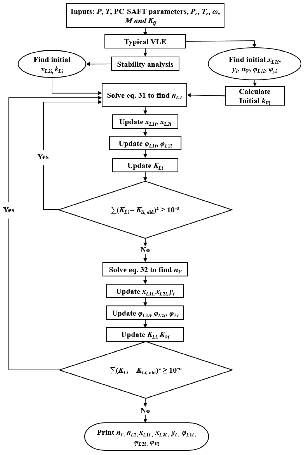
This algorithm efficiently solves the phase equilibrium by solving the three-phase RR equation using PC-SAFT fugacity coefficients instead of the traditional Gibbs free energy minimization method and can accurately predict vapor–liquid–liquid three-phase equilibrium and asphaltene phase envelopes. The algorithm consists of two layers of loops: the inner loop is used to check the convergence of the asphaltene phase equilibrium constant, and the outer loop recalculates the vapor phase equilibrium constant. At the same time, the asphaltene precipitation behavior is predicted through phase stability analysis, and the three-phase equilibrium is solved by combining the double-nested Rachford–Rice equation, which can avoid the iterative divergence problem of the traditional Gibbs free energy minimization method. It greatly improves calculation stability and convergence efficiency and effectively controls numerical calculation errors.

4.1. Phase Stability Analysis

Phase stability analysis is the core pre-step of the RRPC-SAFT algorithm to judge whether asphaltenes precipitate. It is used to verify whether the oil-rich liquid phase obtained by a two-phase vapor–liquid equilibrium flash will split into an asphaltene second liquid phase, and to provide reliable initial values for subsequent three-phase equilibrium calculations. The Michelsen stability determination method is adopted to iteratively solve multiple trial phases and judge the thermodynamic stability of the system.

4.1.1. Trial Phase Initial Values

Obtain the oil-rich liquid phase composition x_Li and vapor phase composition y_Vi to judge whether the asphaltene phase will precipitate and to provide initial composition guesses for subsequent calculations. Six sets of trial phase compositions Y_i are used for stability analysis to determine whether there is a possible state with lower Gibbs free energy than the single phase:

$$Y_i=z_i{K}_i$$

(18)

$$Y_i=z_i/K_i$$

(19)

$$Y_i=\left(x_{Li}+y_{Vi}\right)/2$$

(20)

$$Y_i=\exp \left(h_i\right)$$

(21)

$$\left\{\begin{array}{c}{Y}_1=0.999\\ Y_i=0.001/\left(N_c-1\right), i=2,3,\dots ,N_c\end{array}\right.$$

(22)

$$\left\{\begin{array}{c}{Y}_i=0.001/\left(N_c-1\right), i=1,2,\dots ,N_c-1\\ Y_{Nc}=0.999\end{array}\right.$$

(23)

where K_i is the equilibrium constant, h_i is calculated through the fugacity coefficient φ_i and the total composition z_i, and the fugacity coefficient is also calculated based on the total composition:

$$h_i=\ln z_i+\ln ({\phi }_i)$$

(24)

4.1.2. Convergence and Stability Judgment

The residual criterion for the trial phase iterative convergence is:

$$\max \left|r_i\right|=\max \left|\ln Y_i+\ln {\phi }_i(y)-h_i\right|<{10}^{-8}$$

(25)

where Y_i is the trial phase composition; φ_i(y) is the component fugacity coefficient of the trial phase.

After convergence, two core verifications need to be completed. First, check whether the solution of the algorithm is a non-trivial solution to avoid converging to the composition of the existing phase. The criterion is:

$${\left[{\displaystyle \sum _{i=1}^{N_c}{(y_i-C_i)}^2}\right]}^{{\displaystyle \frac{1}{2}}}\ge {\displaystyle \frac{{\epsilon }_{\mathrm{trivial}}}{N_c}}$$

(26)

where ε_trivial (10⁻⁸), and C_i are sequentially replaced by the total feed composition z_i, the oil-rich liquid phase composition x_Li, and the vapor phase composition y_Vi. If the solution is a trivial solution or does not converge within the preset maximum number of iterations, replace the initial value of Y_i for subsequent calculation.

Then perform the final stability judgment: if the following formula is satisfied, it is judged that the oil-rich liquid phase is thermodynamically unstable and will precipitate a second liquid asphaltene phase:

$$\left|{\displaystyle \sum _{i=1}^{N_c}{Y}_i}-1\right|\ge {10}^{-8}$$

(27)

The trial phase composition y_i that meets this convergence condition is the initial composition x_L2i of the asphaltene phase; if all trial phases do not meet the above conditions, it is established that the liquid phase is stable and no asphaltene precipitation occurs.

4.2. Three-Phase VLLE Calculation

The PC-SAFT asphaltene phase diagram prediction algorithm based on the three-phase Rachford–Rice equation solves the three-phase RR equation simultaneously through double-nested loops instead of the traditional Gibbs free energy minimization method, thereby achieving an efficient solution of the three-phase equilibrium of asphaltene systems.

The crude oil equilibrium system is divided into three phases: the vapor phase, the oil-rich liquid phase, and the asphaltene-rich liquid phase. The total mole fraction of the system satisfies the normalization condition:

$$V+L_1+L_2=1$$

(28)

where V, L₁, L₂ are the mole fractions of the vapor phase, oil-rich liquid phase, and asphaltene-rich liquid phase at equilibrium, respectively. Taking 1 mol as the benchmark, L₁ and L₂ are the amounts of substance of the oil-rich liquid phase and asphaltene-rich phase, respectively. The phase equilibrium constant is defined as:

$$K_{Vi}={\displaystyle \frac{y_i}{x_{L1i}}}={\displaystyle \frac{{\phi }_{L1i}}{{\phi }_{Vi}}}$$

(29)

$$K_{Li}={\displaystyle \frac{x_{L2i}}{x_{L1i}}}={\displaystyle \frac{{\phi }_{L1i}}{{\phi }_{L2i}}}$$

(30)

where K_Vi is the vapor–liquid equilibrium constant; K_Li is the liquid–liquid (asphaltene phase) equilibrium constant; x_L2i is the mole fraction of component i in the asphaltene-rich liquid phase; φ_Vi, φ_L1i, φ_L2i are the fugacity coefficients of component i in the vapor phase, oil-rich liquid phase, and asphaltene-rich liquid phase, respectively.

First, perform a vapor–liquid equilibrium (VLE) flash calculation on the system to obtain the initial value of the vapor phase equilibrium constant K_Vi, then perform phase stability analysis of the liquid phase composition to obtain the asphaltene phase equilibrium constant K_Li. If the stability analysis result indicates that the system will form an asphaltene phase, complete the VLLE calculation. To solve the double three-phase RR equations of the asphaltene second liquid phase and vapor phase, realize the simultaneous solution of material conservation and phase equilibrium, in the following form:

$$R{R}_1={\displaystyle {\displaystyle \sum _{i=1}^{N_c}}(y_i-x_{L1i})}s={\displaystyle {\displaystyle \sum _{i=1}^{N_c}}\frac{z_i\left(K_{Vi}-1\right)}{1+V\left(K_{Vi}-1\right)+L_2\left(K_{Li}-1\right)}}=0$$

(31)

$$R{R}_2={\displaystyle {\displaystyle \sum _{i=1}^{N_c}}(x_{L2i}-x_{L1i})}={\displaystyle {\displaystyle \sum _{i=1}^{N_c}}\frac{z_i\left(K_{Li}-1\right)}{1+V\left(K_{Vi}-1\right)+L_2\left(K_{Li}-1\right)}}=0$$

(32)

where z_i is the total feed mole fraction of component i. The denominator represents the coupling term between the phase fraction and the equilibrium constant. The flowchart of the vapor–liquid–liquid equilibrium (VLLE) algorithm is shown in Figure 2.

5. Results and Discussion

Based on the RRPC-SAFT model and the three-phase VLLE fast solution algorithm, three typical field crude oil systems were selected: high gas-oil ratio black oil reservoir A [35], high CO₂-content reservoir B [35], and light low-asphaltene reservoir C [23], to carry out comprehensive verification of three core indicators: bubble point pressure, asphaltene onset precipitation pressure (AOP), and phase state partition characterization. On this basis, reservoir B was selected as the research object to stimulate the asphaltene deposition phase behavior under three mainstream gas injection media (N₂, CH₄, and CO₂); reservoir C was selected as the research object to investigate the sensitivity of SARA four components using the single-factor variable control method, and the influence laws of different factors on the critical conditions and deposition intensity of asphaltene deposition was quantified.

5.1. High Gas-Oil Ratio Black Oil Reservoir A

This paper adopts the engineering accuracy criterion for reservoir fluid phase equilibrium simulation: the average relative errors of bubble point pressure and asphaltene onset pressure (AOP) are ≤ 5%, and meeting this threshold is deemed to satisfy the requirements of on-site engineering calculation. All subsequent model error evaluations follow this quantitative criterion.

Reservoir A is a conventional black oil reservoir system with a high gas-oil ratio [35], and four PVT testing methods, namely, the gravimetric method, the acoustic resonance technique (ART), near-infrared (NIR) spectroscopy, and the filtration method, are adopted with test temperatures covering 99–116 °C. Parameter fitting is conducted based on data at a single temperature point, and data at other temperatures are used for independent validation; the measurement is dominated by NIR light scattering, with a measurement error of ±1.7237 MPa for asphaltene precipitation pressure. The basic fluid components and characterization results of different models are shown in

Table 5. Fluid components of reservoir A.

Component	Mole Fraction (%)
N2	0.48
CO2	0.92
H2S	0.00
C1	43.43
C2	11.02
C3	6.55
iC4	0.79
nC4	3.70
iC5	1.28
nC5	2.25
C6	2.70
C7+	26.88
C7+ molar mass (g/mol)	228.1
C7+ density (g/cm3), 0.101 MPa, 15 °C	0.865

,

Table 6. Characterization results of oil components of reservoir A for PR equation of state.

Component	Molar Mass (g/mol)	Mole Fraction (%)	Critical Temperature Tc (°C)	Critical Pressure Pc (MPa)	Acentric Factor ω
N2	28.0	0.480	−146.95	3.3940	0.04
CO2	44.0	0.919	31.05	7.3760	0.225
C1	16.0	43.391	−82.55	4.6000	0.008
C2	30.1	11.010	32.25	4.8840	0.098
C3	44.1	6.544	96.65	4.2460	0.152
iC4	58.1	0.789	134.95	3.6480	0.176
nC4	58.1	3.787	152.05	3.8000	0.193
iC5	72.2	1.279	187.25	3.3840	0.227
nC5	72.2	2.248	196.45	3.3740	0.251
C6	86.2	2.698	234.25	2.9690	0.296
C7–C25	180.4	22.738	418.66	1.9460	0.6803
C26–C49	460.3	3.747	683.62	1.3080	1.2077
C50–C64	769.2	0.230	845.45	1.0660	0.9492
C50–C64-A	769.2	0.070	1172.58	1.7300	1.274
C65–C80	982.8	0.054	1051.88	1.0280	0.1823
C65–C80-A	982.8	0.016	1172.58	1.7300	1.274

and

Table 7. PC-SAFT characterization results of reservoir A fluid.

Component	Molar Mass (g/mol)	Mole Fraction (%)	Segment Number m	Segment Diameter σ (Å)	Segment Energy Parameter ε/k (K)
N2	28.01	0.48	1.206	3.313	90.96
CO2	44.01	0.92	2.073	2.785	169.21
C1	16.04	43.43	1.000	3.704	150.03
C2	30.07	11.02	1.607	3.520	191.42
C3	44.10	6.55	2.002	3.618	208.11
Heavy gas	69.81	10.72	2.64	3.75	258
Saturates	210.63	14.72	6.24	3.92	256
A + R	250.070	9.67	6.32	4.12	295
Asphaltenes	1700	0.0676	29.5000	4.3000	420.00

. In the PR and SRK models, the binary interaction parameters between asphaltene components and C₁–C₉ hydrocarbons are defaulted to 0.017, and the binary interaction parameters between all other hydrocarbons are defaulted to 0, as shown in

Table 8. Binary interaction parameters in cubic equations of state.

Component	N2	CO2	H2S	C1–C9
CO2	−0.032	-	-	-
H2S	0.170	0.099	-	-
C1	0.028	0.120	0.080	-
C2	0.041	0.120	0.085	-
C3	0.076	0.120	0.089	-
iC4	0.094	0.120	0.051	-
nC4	0.070	0.120	0.060	-
iC5	0.087	0.120	0.060	-
nC5	0.088	0.120	0.069	-
C6	0.080	0.120	0.050	-
C7	0.080	0.100	-	-
C7+-A	0.080	0.100	-	0.017

.

The measured bubble point pressure and AOP data at 99 °C are selected as the parameter calibration dataset to complete the matching of aromaticity γ and asphaltene parameters. The bubble point and AOP data at three temperatures of 104 °C, 110 °C, and 116 °C are all independent validation data, and no model parameters are adjusted after parameter calibration.

The PR and RRPC-SAFT models were used for a multi-dimensional performance comparison, and the bubble point pressure prediction results and error statistics are shown in

Table 9. Comparison of bubble point pressure prediction results of reservoir A fluid at different temperatures.

T (°C)	Measured Value P (MPa)	PR		RRPC-SAFT
		Predicted Value (MPa)	Relative Error (%)	Predicted Value (MPa)	Relative Error (%)
99	22.21	22.9	3.1067	21.74	2.1162
104	22.64	22.9	1.1484	22.1	2.3852
110	22.59	23.4	3.5857	22.33	1.1510
116	22.68	24	5.8201	22.8	0.5291
Average relative error	-	-	3.4152	-	1.5453

. The bubble point prediction errors of both models are at a low level, among which the average relative error of the RRPC-SAFT model is 1.5453%, meeting the engineering accuracy criterion of ≤5%; the average relative error of the PR model is 3.4152%, which also satisfies the engineering accuracy requirements. The error of the PR model tends to increase with the rise in temperature, reaching a relative error of 5.8201% under a high-temperature condition of 116 °C; the error fluctuation range of the RRPC-SAFT model over the full temperature range is 1.8571%, with more stable accuracy performance in the high-temperature interval. The PR model, based on the mean field theory, cannot accurately describe the high-temperature vapor–liquid equilibrium law of high gas-oil ratio asymmetric systems, while the RRPC-SAFT model can accurately characterize the intermolecular interactions between light hydrocarbons and heavy components at different temperatures.

The prediction results of AOP are shown in

Table 10. AOP prediction results of reservoir A fluid at different temperatures.

T (°C)	Measured Value P (MPa)	PR		RRPC-SAFT
		Predicted Value (MPa)	Relative Error (%)	Predicted Value (MPa)	Relative Error (%)
99	47.26	46.5	1.6081	47.1	0.3386
104	45.42	45	0.9247	45.7	0.6165
110	44.26	43.3	2.1690	44.5	0.5423
116	42.92	42	2.1435	42.8	0.2796
Average relative error	-	-	1.7113	-	0.4442

. The average relative error of AOP for the RRPC-SAFT model is 0.4442%, and that for the PR model is 1.7113%, both of which meet the engineering accuracy criterion of ≤5%; the predicted values of the PR model over the full temperature range are generally lower than the measured values, while the RRPC-SAFT model shows no obvious systematic deviation.

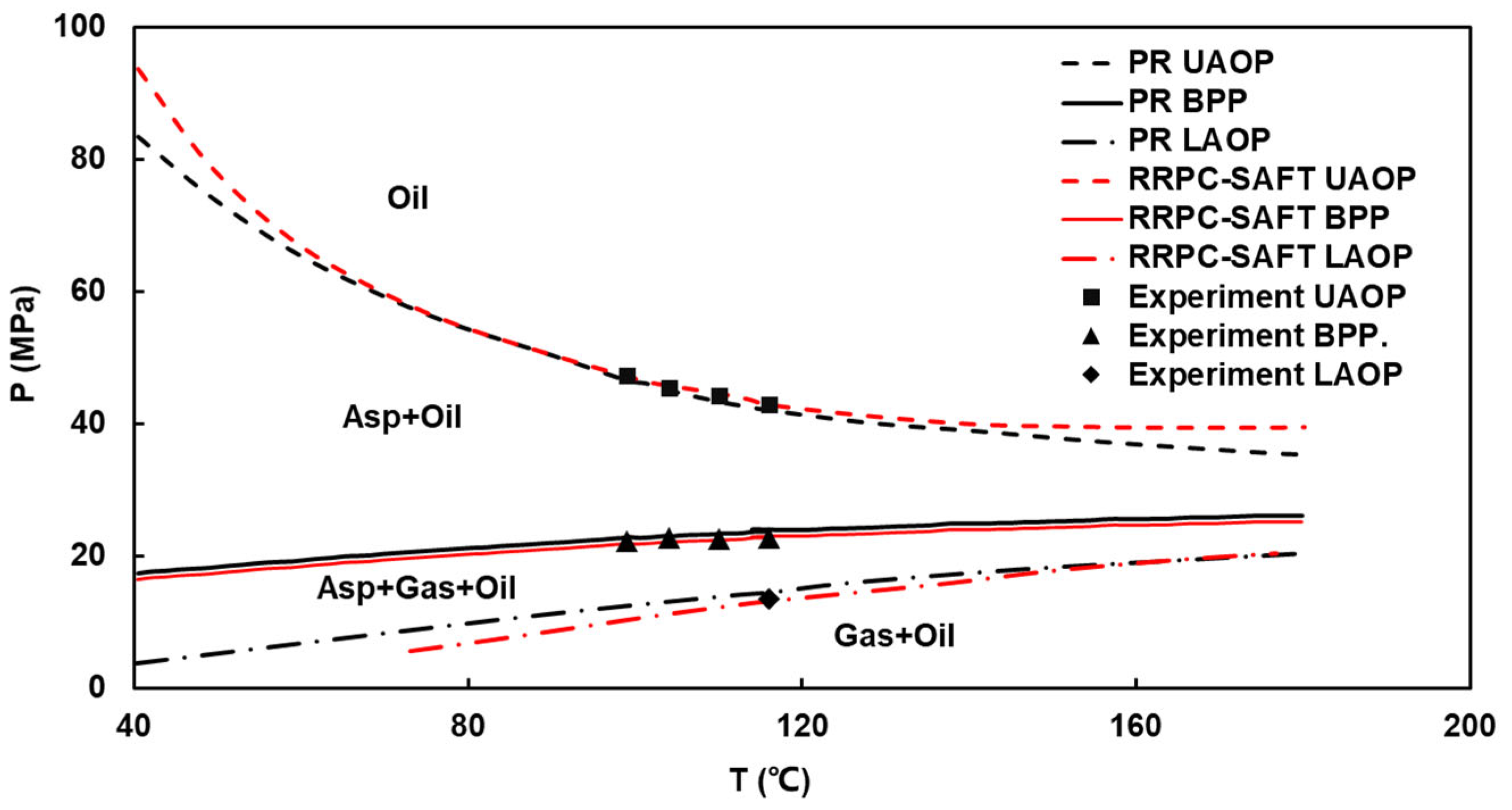
Based on the phase equilibrium calculation results of the PR and RRPC-SAFT equations of state (Figure 3), the asphaltene instability zone predicted by the PR model is small, and the precipitation pressure prediction is low in the low-temperature interval; the upper and lower precipitation pressure lines predicted by the RRPC-SAFT model are highly consistent with the experimental measurement points, with the relative error of the upper precipitation pressure prediction controlled within 1%, and the overall error across the entire temperature range being less than 3%.

5.2. High CO₂ Reservoir B

Reservoir B is a typical oil reservoir with high CO₂ content, with a CO₂ mole fraction of 11.37% [35]. The reference test temperature is 82 °C, consistent with the testing method for Reservoir A. The measured bubble point pressure and AOP data at 120 °C are selected as the parameter calibration dataset; the bubble point and AOP data at three temperatures of 83.2 °C, 104.2 °C, and 141.1 °C, as well as all N₂ gas injection scenarios and comparative scenarios with different injection media, were all independent validation data, and no model parameters were modified throughout the process.

The SRK and RRPC-SAFT models were used for a multi-dimensional performance comparison, and the bubble point pressure prediction results and error statistics are shown in

Table 11. Comparison of bubble point pressure prediction results of reservoir B fluid at different temperatures.

T (°C)	Measured Value P (MPa)	SRK		RRPC-SAFT
		Predicted Value (MPa)	Relative Error (%)	Predicted Value (MPa)	Relative Error (%)
83.2	17.24	17.43	1.1021	17.5	1.5081
104.2	18.62	18.91	1.5575	18.99	1.9871
120	19.99	19.92	0.3502	20.03	0.2001
141.1	21.1	21.06	0.1896	20.98	0.5687
Average relative error	-	-	0.7998	-	1.0660

. The average relative errors of bubble point prediction of both models are lower than 2%, meeting the engineering accuracy criterion of ≤5%; among them, the average relative error of the SRK model is 0.7998%, slightly lower than 1.0660% of the RRPC-SAFT model, and the two models have close accuracy with no obvious systematic deviation. The error increases with decreasing temperature, and the accuracy is highest in the formation temperature range of 120.0~141.1 °C, with average relative errors of 0.2699% and 0.3844%, respectively. The fugacity of CO₂ and the light hydrocarbon liquid phase are more sensitive to the accuracy of intermolecular interaction description at low temperatures, and the SRK model has a mature empirical parameter correction system for hydrocarbon-CO₂ systems, so it shows a slight advantage in the low-temperature interval.

The prediction results of AOP are shown in

Table 12. AOP prediction results of reservoir B fluid at different temperatures.

T (°C)	Measured Value P (MPa)	SRK		RRPC-SAFT
		Predicted Value (MPa)	Relative Error (%)	Predicted Value (MPa)	Relative Error (%)
83.2	37.23	33.99	8.7027	38.5	3.4112
104.2	27.92	29.01	3.9040	29	3.8682
120	25.17	26.51	5.3238	26.2	4.0922
141.1	26.2	24.61	6.0687	25	4.5802
Average relative error	-	-	5.9998	-	3.9879

. The average relative error of the RRPC-SAFT model is 3.9879%, meeting the engineering accuracy criterion of ≤5%; the average relative error of the SRK model is 5.9998%, exceeding the engineering accuracy threshold. The relative error of the SRK model reaches 8.7027% under the low-temperature condition of 83.2 °C, with a wider error fluctuation range; the maximum relative error of the RRPC-SAFT model over the full temperature range is 4.5802%, with more stable accuracy performance. The core mechanism is that the RRPC-SAFT model can accurately characterize the dispersion interaction between asphaltene macromolecular chains and small molecules, thereby compensating for the inherent defects of the SRK model based on the mean field theory.

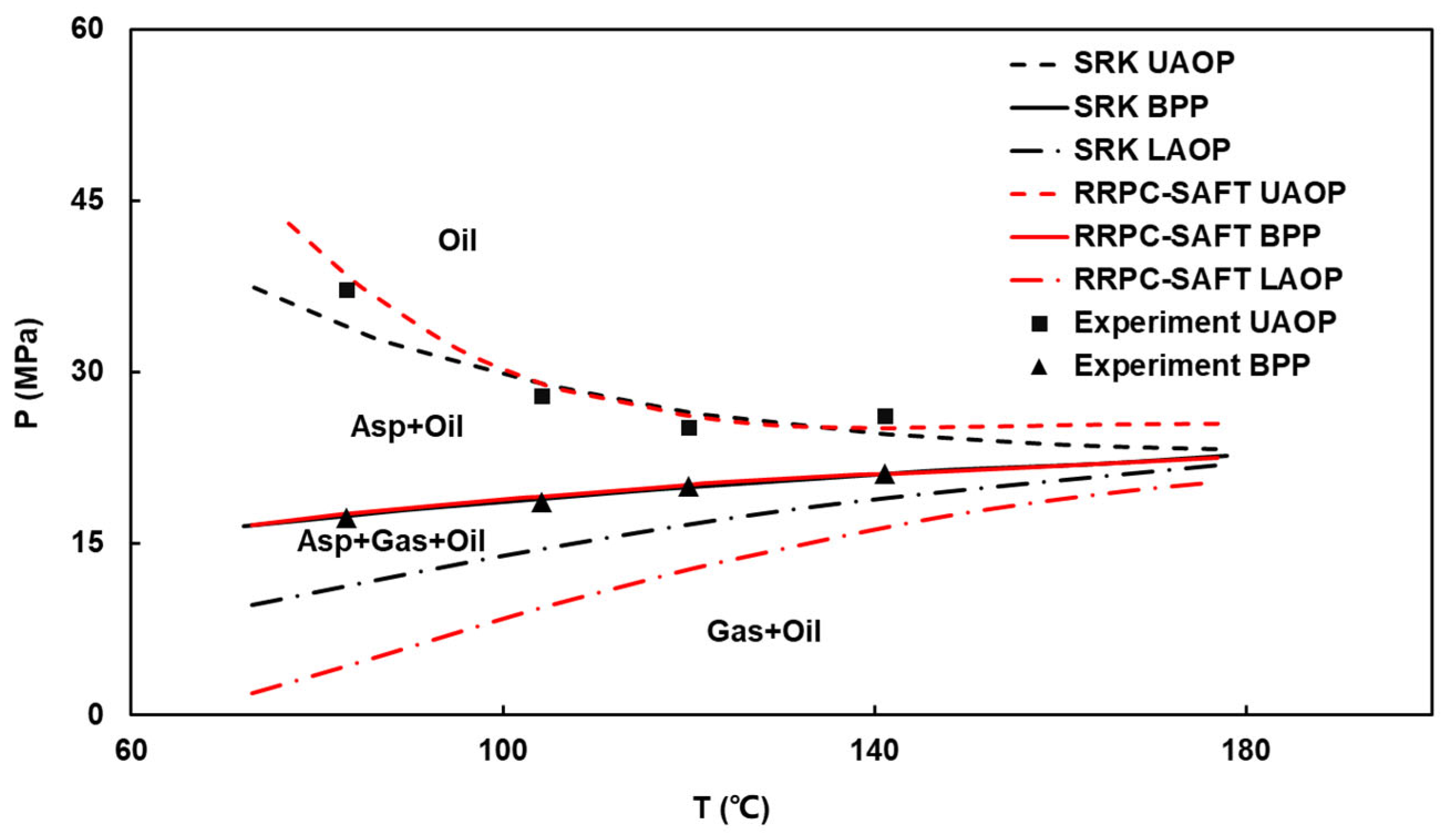
Based on the phase equilibrium calculation results of the SRK and RRPC-SAFT equations of state (Figure 4), the asphaltene instability zone predicted by the SRK model is significantly smaller than the measured results, and cannot accurately describe the increasing trend of the lower precipitation pressure with temperature and the low-temperature re-dissolution behavior. The RRPC-SAFT model exhibits stable calculation performance over the full temperature range of 80–180 °C, with the average relative error of asphaltene precipitation pressure prediction controlled within 5%, and shows better agreement with the measured precipitation envelope.

The RRPC-SAFT calculation framework established in this paper has clear engineering value for the integrated development of CO₂-EOR and CCUS. CO₂ injection disrupts the colloidal equilibrium of crude oil, induces asphaltene precipitation that can plug pore throats and wellbores, and damages reservoir permeability, which is a core problem restricting carbon storage and gas injection recovery efficiency [3]. The simulation results in this paper for high-CO₂ reservoirs can quickly determine the critical conditions of asphaltene precipitation under different gas injection volumes, and provide a thermodynamic basis for on-site gas injection schemes and flow assurance management.

In terms of multi-scale reservoir damage, asphaltene has two plugging modes, namely, surface adsorption and pore throat bridging. Microscopic pore simulation requires macroscopic phase equilibrium results as boundary conditions, and the high-precision phase equilibrium data in this paper can provide reliable input for pore-scale damage simulation [3].

From the perspective of prevention and control technologies, current research on asphaltene inhibitors has investigated the mechanism of molecular interaction, and asphaltene dispersion is achieved through hydrogen bonds and van der Waals forces. There are differences in the types of inhibitors suitable for different asphaltene molecules [36]. The SARA fraction perturbation simulation in this paper can be used to pre-screen inhibitors and reduce experimental costs.

5.3. Light Low-Asphaltene Reservoir C

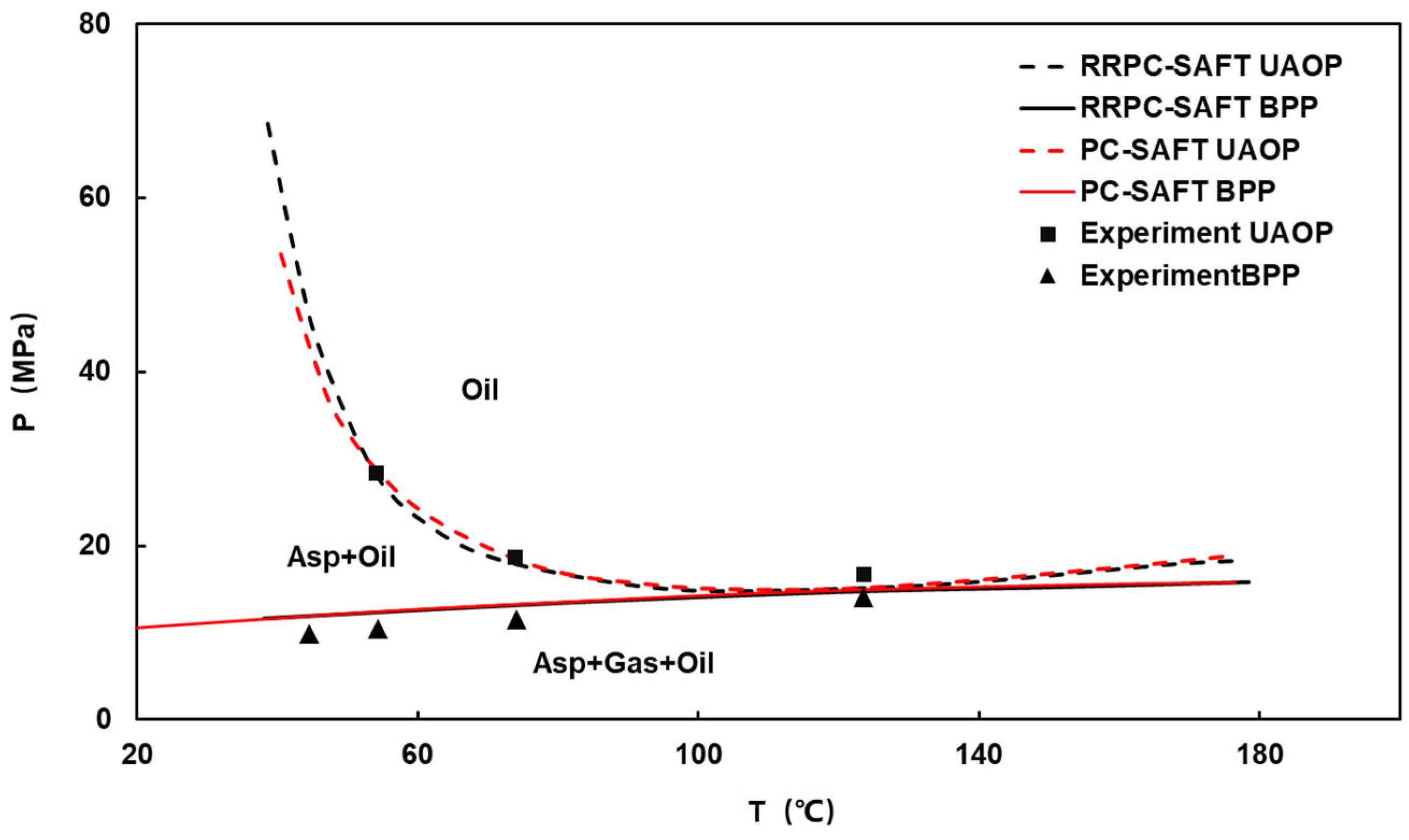
Reservoir C is a light crude oil system with low asphaltene content [23], the experimental fluids and corresponding PVT, SARA, and gas injection experimental data are provided by Abu Dhabi National Oil Company (ADNOC), and the near-infrared (NIR) light scattering method is adopted with multiple temperature gradients set from 44.56 °C to 123.56 °C. The PC-SAFT and RRPC-SAFT models were used for multi-dimensional performance comparison, and the bubble point pressure prediction results and error statistics are shown in

Table 13. Comparison of bubble point pressure prediction results of reservoir C fluid at different temperatures.

T (°C)	Measured Value P (MPa)	PC-SAFT		RRPC-SAFT
		Predicted Value (MPa)	Relative Error (%)	Predicted Value (MPa)	Relative Error (%)
44.56	9.9	10.26	3.6364	10.67	7.7778
54.36	10.44	10.91	4.5019	11.12	6.5134
74.09	11.53	11.96	3.7294	12.01	4.1631
123.56	14.11	13.93	1.2757	13.99	0.8505
Average relative error	-	-	3.2858	-	4.8262

. The measured bubble point pressure and AOP data at 74.09 °C were selected as the parameter calibration dataset; the bubble point and AOP data at temperatures of 44.56 °C, 54.36 °C, and 123.56 °C, as well as the subsequent SARA four-fraction perturbation scenarios, were all independent validation data without secondary parameter tuning.

The average relative errors of both models over the full temperature interval are controlled within 5%, with a difference of only 1.5404%, confirming that the RRPC-SAFT algorithm does not degrade prediction accuracy for vapor–liquid two-phase equilibrium. The error decreases significantly with increasing temperature, and at 123.56 °C formation temperature, the relative error of the RRPC-SAFT model is only 0.8505%, surpassing that of the traditional model.

The prediction results of AOP are shown in

Table 14. AOP prediction results of reservoir C fluid at different temperatures.

T (°C)	Measured Value P (MPa)	PC-SAFT		RRPC-SAFT
		Predicted Value (MPa)	Relative Error (%)	Predicted Value (MPa)	Relative Error (%)
54.36	28.35	28.16	0.6619	28.19	0.5561
74.09	18.72	18.34	2.0172	17.88	4.4748
123.56	15.90	15.24	4.1264	15.28	3.8747
Average relative error	-	-	2.2685	-	2.9685

. The difference in average relative error between the two models is only 0.699%, and both meet the engineering accuracy criterion of ≤5%. The RRPC-SAFT algorithm completely retains the high-precision prediction characteristics of the traditional PC-SAFT model. The errors of both models increase slightly in the 74.09 °C medium-temperature interval because this temperature corresponds to the slope inflection point of the precipitation envelope; the errors of both models drop to about 4% at formation temperature, meeting the engineering accuracy requirements.

Over the entire temperature interval, both the RRPC-SAFT model and the traditional PC-SAFT model show extremely high prediction accuracy for AOP, with a difference in average relative error of only 0.699%. Combined with the crude oil bubble point line and asphaltene deposition envelope (Figure 5), these results confirm that the prediction accuracy of the RRPC-SAFT algorithm for asphaltene phase behavior is on par with that of the conventional PC-SAFT model, achieving a balance between calculation accuracy and efficiency.

The summary of error data for the three types of crude oil is shown in

Table 15. Summary of Model Performance for the Three Crude Oil Systems.

Reservoir Type	Index	Comparative Model	Average Error of RRPC-SAFT (%)	Average Error of Comparative Model (%)	Performance Comparison
High Gas-Oil Ratio Black Oil	BPP	PR	1.5453	3.4152	RRPC-SAFT performs better
	AOP	PR	0.4442	1.7113	RRPC-SAFT performs better
High CO2 Crude Oil	BPP	SRK	1.0660	0.7998	Comparable
	AOP	SRK	3.9879	5.9998	RRPC-SAFT performs better
Light Crude Oil with Low Asphaltene Content	BPP	Conventional PC-SAFT	4.8262	3.2858	Comparable
	AOP	Conventional PC-SAFT	2.9685	2.2685	Comparable

. Classical cubic equations of state such as PR and SRK have inherent advantages in the calculation of vapor–liquid bubble point equilibrium of conventional hydrocarbons, owing to long-term industrial data accumulation, parameter optimization, and a well-established empirical correction system. The RRPC-SAFT model proposed in this paper focuses on liquid–liquid equilibrium systems with molecular asymmetry and macromolecules, and is suitable for asphaltene deposition simulation scenarios. The differences in their theoretical positioning and original design intentions lead to differences in computational performance. The comprehensive simulation results show that the RRPC-SAFT model has a lower overall error in predicting asphaltene phase instability. For vapor–liquid bubble point calculation, the two types of models have their own advantages and disadvantages for different fluid systems, and an appropriate thermodynamic model should be selected according to the calculation objective and fluid type.

This paper strictly distinguishes the parameter calibration dataset from the independent validation dataset. For each group of crude oil, only experimental data at a single temperature point are used to fit the adjustable parameters, and all other working conditions are independent predictions without parameter correction, effectively avoiding the risk of overfitting and endowing the model prediction results with reliable generalization capability.

5.4. Influence of Gas Injection Development on Asphaltene Deposition

Gas injection flooding is the core technology for enhanced oil recovery in deep and low-permeability reservoirs. However, injected gas changes the component balance and dissolution capacity of the crude oil system, destabilizes the colloidal stability system of asphaltenes, and thus induces asphaltene instability, flocculation, and deposition. Based on the RRPC-SAFT model, using the high-CO₂ crude oil from reservoir B as the research object, the influence of different injection media and mole fractions on the asphaltene phase equilibrium was quantitatively characterized, and the deposition risk level and action mechanism were clarified.

5.4.1. Influence of N₂ on Asphaltene Phase Equilibrium

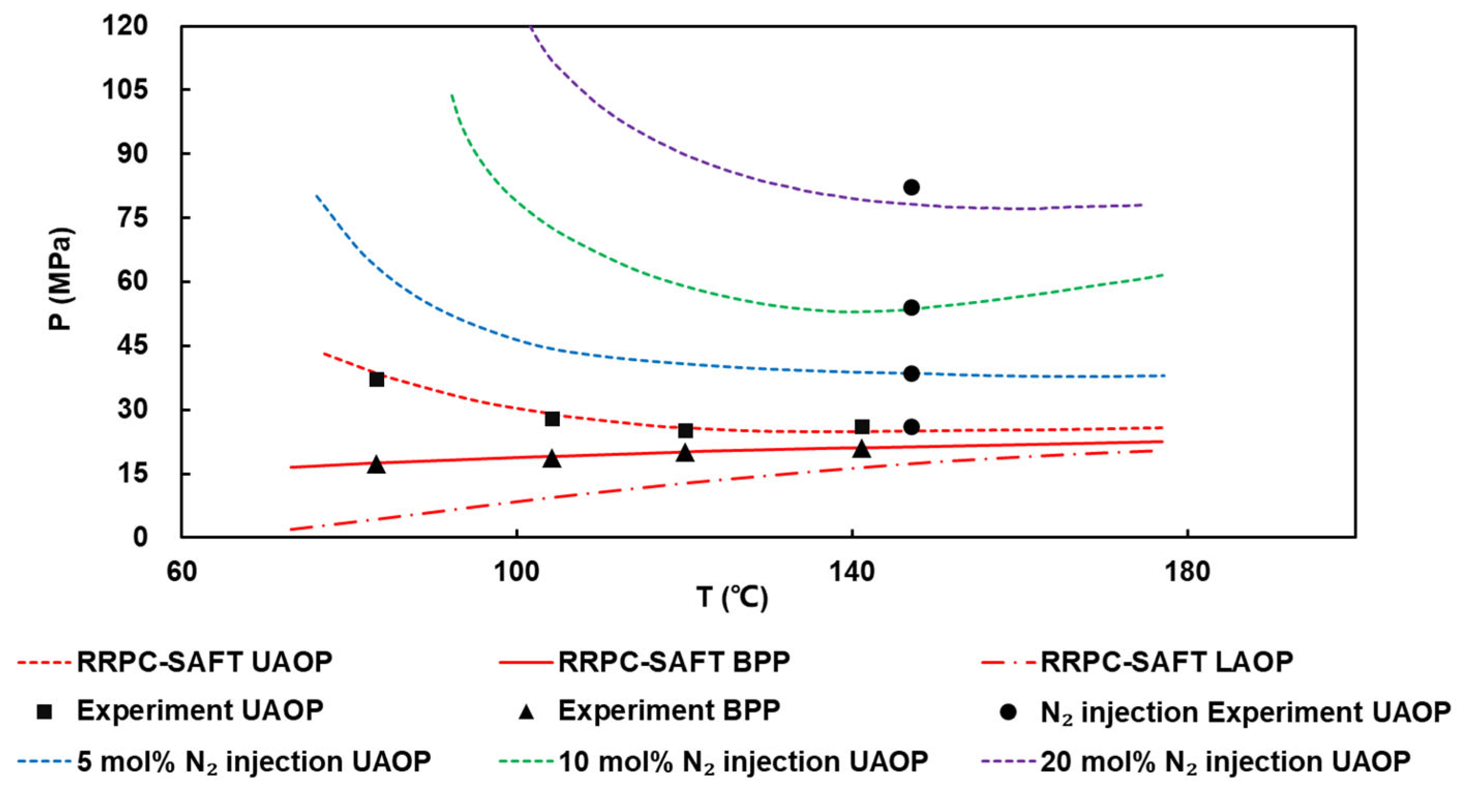
N₂, as a non-polar inert gas, has extremely poor miscibility with crude oil hydrocarbon components and is one of the media with the highest asphaltene deposition risk in gas injection development. At the reservoir temperature of 147 °C, four N₂ injection gradients of 0, 5, 10, and 20 mol% were set to simulate the variation in AOP, and the results are shown in

Table 16. Experimental values of AOP under different N₂ injection ratios of reservoir B fluid at 147 °C.

Injected N2 Mole Percentage (mol%)	Experimental Value of AOP (MPa)	Predicted Value of AOP (MPa)	Relative Error (%)
0	26.70	25.03	1.1236
5	38.64	38.58	0.1553
10	54.10	53.80	0.5545
20	82.20	78.26	4.7932

.

The AOP increases continuously with the increase in N₂ injection volume, and the maximum relative prediction error of the model is 4.7932%, which meets the engineering accuracy criterion of ≤5%. Under the non-gas injection baseline condition, the measured AOP of crude oil is 26.70 MPa; when 5 mol% N₂ is injected, AOP rises to 38.64 MPa, with an absolute increment of 11.94 MPa and a relative increase of 44.72%; when 20 mol% N₂ is injected, the increase in AOP relative to the baseline reaches 207.87%, and the promotion effect of N₂ on asphaltene deposition intensifies continuously with rising injection molar fraction.

To further clarify the influence of N₂ injection on the asphaltene phase behavior envelope over the full temperature interval, the calibrated RRPC-SAFT model was used for phase state prediction. The bubble point lines and asphaltene deposition envelopes of crude oil under different N₂ injection ratios are shown in Figure 6.

As the N₂ injection ratio increases, the asphaltene deposition envelope expands toward the high-temperature and high-pressure zone, and this evolution pattern is consistent with the results of visual gas injection tests [37]. The upper limit of deposition pressure rises with increasing injection ratio; its peak value is below 45 MPa at 0 mol% injection and exceeds 120 MPa at 20 mol%. The asphaltene instability window is significantly widened. The deposition risk spans the entire range of conventional reservoir development; therefore, deposition damage cannot be completely avoided by maintaining formation pressure alone.

The mechanism of action is as follows: N₂ does not interact with asphaltenes and resins but only reduces the solvation capacity of crude oil through a dilution effect, destroying the stable structure of asphaltene micelles. At the same time, the low solubility of N₂ exacerbates changes in light hydrocarbon fugacity in crude oil, further reducing the solubility of asphaltenes and inducing large-scale flocculation and deposition.

5.4.2. Comparative Analysis of Different Injection Media

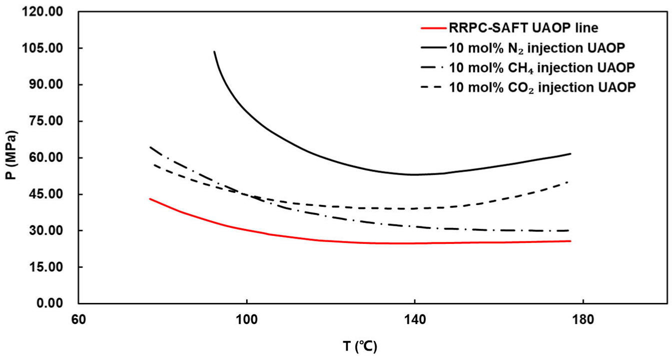
With the injection mole fraction fixed at 10 mol% as a unified variable, parallel comparison simulations of CH₄, CO_2, and N₂ were carried out. The influence of different injection media on asphaltene phase behavior is shown in Figure 7. In the temperature interval of 60–180 °C, after CH₄ and CO₂ injection, the upper AOP values are all located above the asphaltene upper deposition line, indicating that both media raise the asphaltene deposition trigger pressure, but there are significant differences in their influence magnitudes.

There are obvious differences in the phase behavior regulation characteristics of the three media. After CH₄ injection, the deposition envelope shifts slightly upward, the upper precipitation pressure rises to a limited extent, the deposition window widens slightly, and the phase envelope shape is highly similar to that of the baseline crude oil; after CO₂ injection, the deposition envelope shifts moderately upward, the upper precipitation pressure rises significantly more than that observed in CH₄, the deposition window widens obviously, and the low-temperature asphaltene re-dissolution behavior is weakened; after N₂ injection, the deposition envelope shifts greatly upward, the upper precipitation pressure extends into the high pressure range, the deposition window widens globally, and the phase boundary migration amplitude is far greater than those of the first two media.

At the actual reservoir temperature of 147 °C, the predicted asphaltene deposition pressures under 10% N₂, CO_2, and CH₄ injection are shown in

Table 17. Predicted values of AOP under different gas injection conditions.

Gas Injection Situation	Predicted AOP (MPa)	Relative Increase (%)
-	25.03	-
10 mol% CH4	30.86	23.30
10 mol% CO2	39.62	58.30
10 mol% N2	53.80	114.94

. Based on the quantitative data under 10 mol% equimolar injection conditions, the precipitation-promoting intensity of the three injection media in oil fields on asphaltene deposition is ranked as: N₂ > CO₂ > CH₄. The ranking of asphaltene deposition promotion intensity is consistent with the conclusion of laboratory gas injection experiments conducted by Jamaluddin et al. [35]. Their effects on asphaltene deposition differ: CH₄ is a weak precipitation-promoting medium, with an AOP increase of only 23.30%; CO₂ is a moderate precipitation-promoting medium, with an increase of 58.30%; N₂ is a strong precipitation-promoting medium, with an increase of 114.94%.

The core mechanism underlying this difference lies in the different molecular characteristics and compatibility of the injection media with crude oil: CH₄, as the native light hydrocarbon component of crude oil, has excellent miscibility with hydrocarbon components in crude oil [9], and has the weakest weakening effect on the solvation capacity of the crude oil system; the quadrupole moment structure of CO₂ molecules can form weak association with asphaltene polar groups, which alleviates asphaltene aggregation to a certain extent; N₂ is a non-polar inert gas with extremely poor miscibility with crude oil hydrocarbon components, which greatly dilutes the light and resin components of crude oil and significantly reduces the solubility of crude oil for asphaltenes. From the perspective of on-site engineering application, natural gas should be preferentially selected as the injection medium for enhanced oil recovery in this reservoir; if CO₂ flooding is selected as the development method, it is necessary to support the asphaltene inhibitor slug injection process; if N₂ flooding is selected, it is necessary to strictly optimize the injection rate and slug size, and strictly control the underground gas saturation.

5.5. Influence of Saturates on Asphaltene Deposition

Saturates are the components with the highest proportion among the SARA four components of crude oil, and are also poor solvents for asphaltenes. Their content changes will directly change the dissolution capacity of the crude oil system. Using the single-factor variable control method, taking the actual block crude oil of reservoir C as the research object, the regulation mechanism of saturate content on the crude oil phase boundary, AOP, and deposition enrichment degree was systematically revealed.

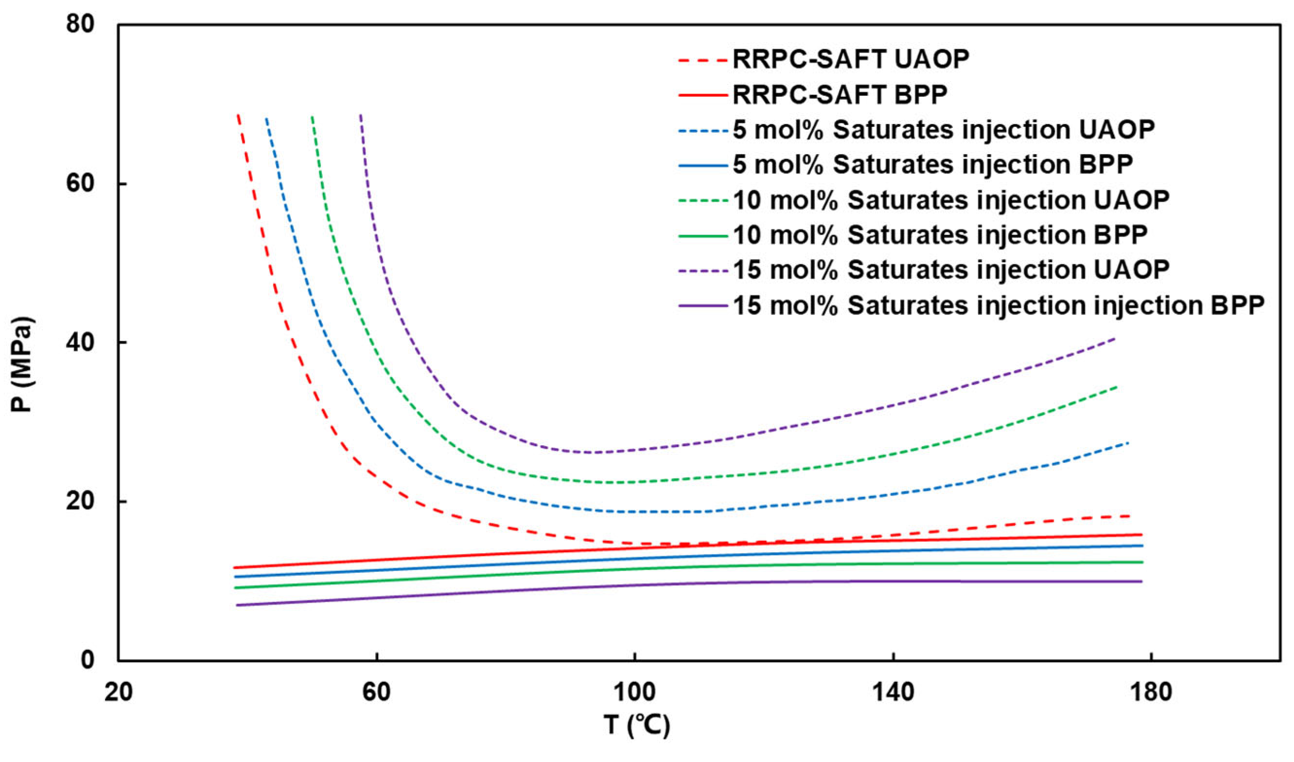
By fixing the mole fraction increment of saturates and compressing all other components in equal proportions according to the original mole ratio, four working conditions were set: baseline crude oil, +5 mol%, +10 mol%, and +15 mol%. The normalized mole composition under each working condition is shown in

Table 18. Mole composition of reservoir C fluid under different saturate increment conditions.

Component	Baseline Oil Composition (mol%)	+5 mol% Saturates	+10 mol% Saturates	+15 mol% Saturates
N2	0.163	0.1552	0.1482	0.1417
CO2	1.944	1.8514	1.7673	1.6904
C1	33.600	32.0000	30.5455	29.2174
C2	7.557	7.1971	6.8700	6.5713
C3	6.742	6.4210	6.1291	5.8626
Heavy gas	8.198	7.8076	7.4527	7.1287
Saturates	31.743	34.9933	37.9482	40.6461
A + R	9.907	9.4352	9.0064	8.6148
Asphaltenes	0.133	0.1267	0.1209	0.1157
Total	100	100	100	100

.

5.5.1. Influence of Saturate Content on Phase Boundary

The phase equilibrium calculation for each working condition was performed using the RRPC-SAFT model. The crude oil bubble point lines and asphaltene deposition envelopes under different saturate contents are shown in Figure 8.

The bubble point pressure shows a continuous decreasing trend with the increase in the saturates’ mole increment, and the decrease in the high-temperature interval is significantly greater than that in the low-temperature interval; under the 15 mol% increment condition, the bubble point pressure is reduced by 12.7% compared with the baseline value, the critical pressure for vapor phase precipitation shifts downward, and the vapor–liquid equilibrium boundary migrates to the low-pressure region. The saturate content is significantly positively correlated with AOP. With an increase in the saturate increment, the AOP across the full temperature interval shows a continuous and significant upward trend, and the asphaltene deposition envelope shifts upward overall; the vertical distance between the deposition line and the bubble point line increases linearly, and the asphaltene deposition pressure window widens globally. Under the 15 mol% increment condition, the AOP rises by more than 120% compared with the baseline value, and the deposition risk interval of crude oil in the single-phase liquid phase region expands by more than three times.

The action mechanism is as follows: saturates occupy the solvent space of A + R, reduce the overall aromaticity of the crude oil system, and weaken the dissolution stability of asphaltene molecules; at the same time, saturates cannot form micelle protective films, thereby accelerating the association and flocculation of asphaltene molecules.

5.5.2. Influence of Saturate Content on Asphaltene Enrichment Degree

By fixing the temperature at 74.1 °C, the asphaltene enrichment degree and relative increase under each working condition were measured, and the results are shown in

Table 19. Asphaltene mass fraction in the precipitated phase.

Working Condition	Mass Fraction of Asphaltenes in the Precipitated Phase (wt.%)	Relative Increase (%)
Baseline crude oil	66.91	-
+5 mol% Saturates	69.85	4.39
+10 mol% Saturates	75.3	12.54
+15 mol% Saturates	83.89	25.38

. The asphaltene deposition intensity is positively correlated with the saturate content, and the increase continues to amplify with the increase in the increment. The increase in enrichment degree is only 4.39% at the 5 mol% increment, reaches 12.54% under the 10 mol% increment, and is as high as 25.38% under the 15 mol% increment, with the enrichment degree exceeding 80 wt.%; the purity of the deposited phase increases, and the corresponding risk of pore plugging rises accordingly. The reason is that the increase in the saturate content further compresses the asphaltene dissolution space, promotes more asphaltene molecules to separate from the oil phase into the asphaltene-rich phase, and at the same time inhibits asphaltene re-dissolution, exacerbating the degree of phase separation.

5.6. Influence of Aromatics + Resins on Asphaltene Deposition

Aromatics and resins are the core components of the crude oil colloid system that maintain the stability of asphaltenes. Aromatics can improve the solubility of asphaltenes through π-π interactions, and resins can inhibit the association of asphaltene molecules through steric hindrance effects. By fixing the mole fraction increment of A + R and compressing all other components in equal proportion according to the original mole ratio, four working conditions were set: baseline crude oil, +5 mol%, +10 mol%, and +15 mol%.

5.6.1. Influence of Aromatics + Resins Content on Phase Boundary

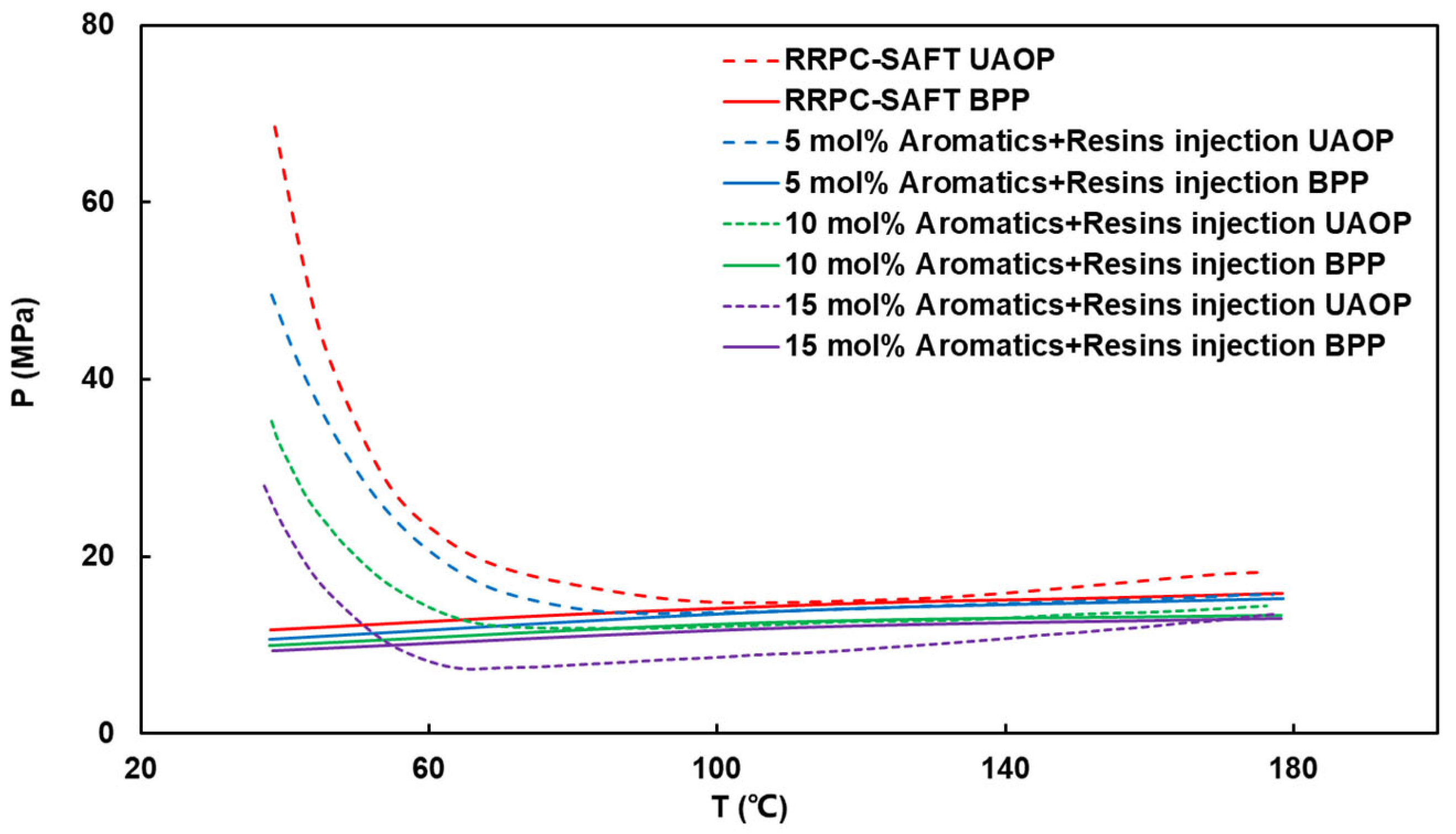
The phase equilibrium calculation for each working condition was completed using the RRPC-SAFT algorithm. The crude oil bubble point lines and asphaltene deposition envelopes under different A + R contents are shown in Figure 9.

Contrary to the trend observed when adding saturates, the AOP decreases significantly overall, and the more A + R are added, the greater the decrease; the decrease in the low-temperature interval is much greater than that in the high-temperature interval, the slope of the deposition line decreases significantly and the curve becomes very flat; the distance between the deposition line and the bubble point line is greatly reduced, and the asphaltene deposition window is significantly narrowed. When the addition amount reaches 15 mol%, the AOP crosses the bubble point line, and theoretically, there is no asphaltene deposition risk in the single-phase region.

5.6.2. Influence of Aromatics + Resins Content on Asphaltene Enrichment Degree

At 74.1 °C, the change in the asphaltene enrichment degree in the liquid–liquid equilibrium asphaltene-rich precipitated phase is shown in

Table 20. Mass fraction of asphaltenes in the asphaltene-rich precipitated phase.

Working Condition	Mass Fraction of Asphaltenes in the Precipitated Phase (wt.%)	Relative Increase Compared to Baseline (%)
Baseline crude oil	66.91	-
+5 mol% A + R	57.64	−13.85
+10 mol% A + R	44.15	−34.02
+15 mol% A + R	25.84	−61.38

. The asphaltene deposition amount is significantly negatively correlated with the content of A + R. As the mole fraction increment of A + R increases from 0 mol% to 15 mol%, the mass fraction of asphaltenes in the asphaltene-rich precipitated phase at the bubble point decreases from 66.91 wt.% to 25.84 wt.%, with a relative decrease of 61.38%, indicating an obvious inhibitory effect on asphaltene deposition.

The action mechanism is as follows: the aromatic rings of aromatics can form strong π-π interactions with the fused aromatic nuclei of asphaltenes, greatly improving the solubility of asphaltenes in the oil phase [38]; the polar ends of resins can be adsorbed on the surface of asphaltene aggregates, and the non-polar ends extend into the oil phase to form a stable solvation film, producing a steric hindrance effect and preventing asphaltene molecules from aggregating and precipitating.

5.7. Influence of Asphaltenes on Asphaltene Deposition

Asphaltenes are the primary constituents involved in deposition behavior, and their initial content in crude oil is the core internal factor determining the critical conditions and intensity of deposition. By fixing the mole fraction increment of asphaltenes and compressing all other components in equal proportion according to the original mole ratio, four working conditions were set: baseline crude oil, +5 mol%, +10 mol%, and +15 mol%.

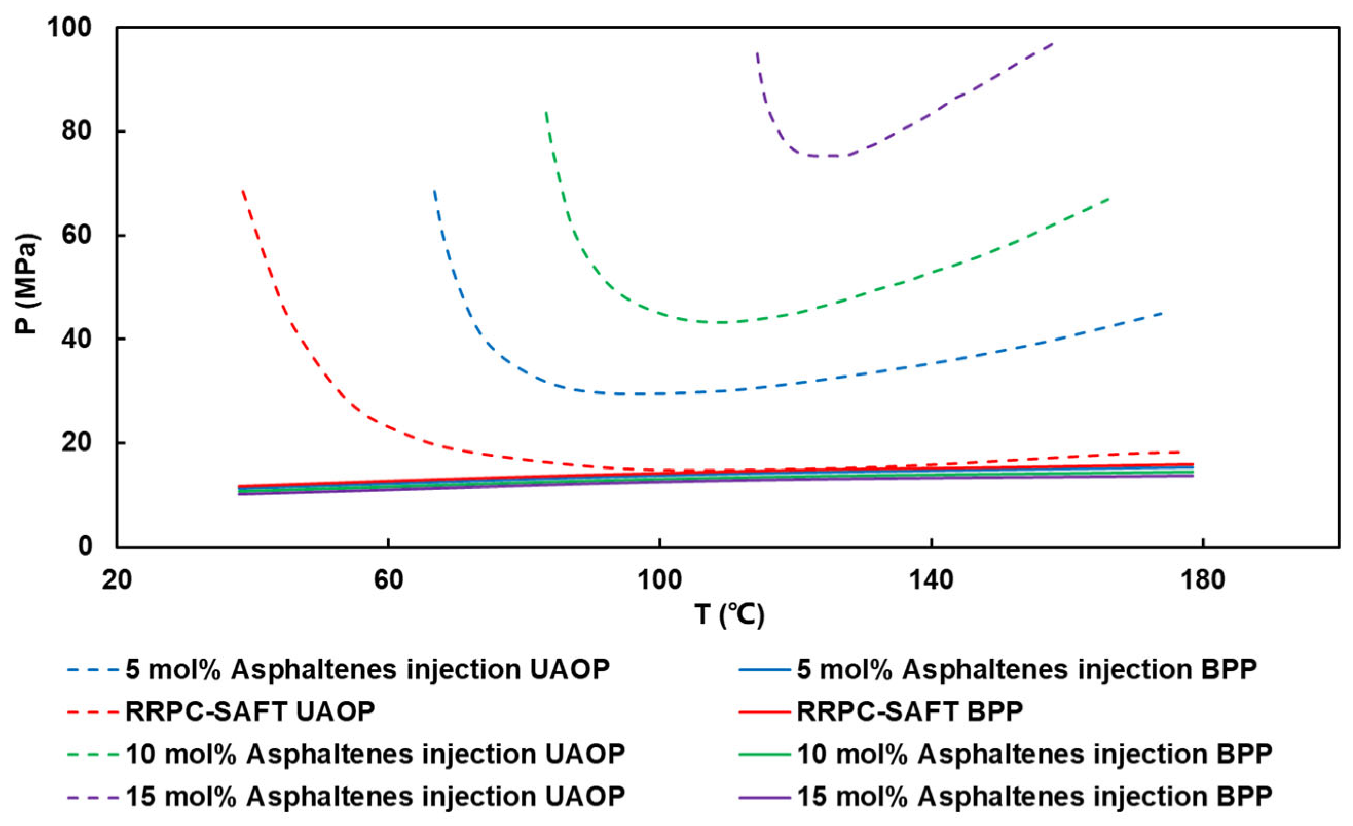
The phase equilibrium calculation for each working condition was completed using the RRPC-SAFT algorithm. The calculation results for the bubble point line and asphaltene deposition line of reservoir C fluid are shown in Figure 10.

With the increase in the amount of the asphaltene addition, the upper asphaltene precipitation pressure shows a sharp upward trend [39] and shifts significantly upward overall; under the +15 mol% asphaltene condition, the AOP rises by over 200% relative to the baseline crude oil sample, and the increase is much greater than that under the same mole increment of saturates. Meanwhile, the gap between the asphaltene onset precipitation curve and the bubble point curve widens significantly, and the asphaltene unstable region expands from a narrow interval near the bubble point directly to an interval far exceeding the original formation pressure of the reservoir; under the +15 mol% asphaltene condition, the AOP exceeds 80 MPa, and the crude oil is in a high-risk state of asphaltene deposition throughout the entire reservoir, wellbore and surface gathering and transportation systems.

The core reason is that the crude oil system has an upper limit on the solubility of asphaltenes, and the asphaltene content directly changes the saturation of the system. When the asphaltene concentration exceeds its solubility limit in crude oil, unstable deposition occurs even under the original formation temperature and pressure conditions.

6. Conclusions and Prospect

6.1. Main Conclusions

Based on the existing PC-SAFT thermodynamic framework, this paper integrates the Panuganti-standardized crude oil characterization method and the Parsaei three-phase Rachford–Rice solution algorithm to establish an integrated RRPC-SAFT engineering calculation workflow. Systematic research was conducted on the mechanism of asphaltene phase equilibrium and the evolution of phase behavior under various working conditions, and the dominant control factors of asphaltene instability under different development conditions were quantified. The main research conclusions are as follows:

(1)

Based on the theoretical framework of the classical PC-SAFT equation of state, multi-pseudo-component parameterization of crude oil is realized via the Panuganti standardization approach, which is further coupled with Parsaei’s three-phase Rachford–Rice solver to establish the integrated workflow. Observations indicate that the computational cost of this algorithm is only one-quarter of that of the Gibbs free energy minimization method.

(2)

Validation using three types of field crude oils verifies the outstanding prediction accuracy and performance advantages of the proposed model. For bubble point pressure calculation, the average relative error of the RRPC-SAFT model ranges from 1.07% to 4.83%, fully complying with the specified engineering accuracy threshold of ≤5%. The model outperforms the PR equation for high gas–oil ratio black oil, achieves comparable accuracy to the SRK equation for high-CO₂ crude oil, and maintains prediction precision close to that of the conventional PC-SAFT model for light crude oil with low asphaltene content. In terms of asphaltene onset pressure (AOP) prediction, the average relative error falls within the range of 0.44–3.99%, which also satisfies the 5% error limit. The RRPC-SAFT model delivers lower AOP prediction errors than both PR and SRK equations for high gas-oil ratio black oil and high-CO₂ crude oil, respectively, and exhibits accuracy equivalent to that of the traditional PC-SAFT model for light low-asphaltene crude oil.

(3)

For the high-CO₂ crude oil System B investigated in this work, gas injection elevates AOP and expands the range of deposition risk. At a molar injection fraction of 10 mol%, the asphaltene precipitation-promoting intensity of the three injected media follows the order: N₂ > CO₂ > CH₄. Injecting 20 mol% nitrogen leads to a 207.87% rise in AOP, making nitrogen the injection medium with the highest deposition risk.

(4)

For the light low-asphaltene crude oil System C in this study, the contents of saturates and asphaltenes are positively correlated with deposition risk. At a 15 mol% incremental fraction, the asphaltene enrichment degree rises by 25.38%, and AOP increases by more than 200%. Aromatics plus resins act as the core stabilizing components; a 15 mol% increment reduces the maximum asphaltene deposition amount by 61.38%, which can effectively narrow the deposition window and eliminate the risk of asphaltene precipitation within the single-phase region.

6.2. Future Outlook

The integrated RRPC-SAFT engineering workflow constructed by combining the Panuganti-standardized crude oil characterization method and the Parsaei three-phase Rachford–Rice solving algorithm in this study can realize risk prediction of asphaltene phase instability in crude oil, and provide a thermodynamic theoretical basis for on-site early warning of asphaltene deposition risks and the formulation of prevention and control schemes. Combined with the research outcomes and field engineering requirements, the following recommendations are proposed for future research and field application:

(1)

Conduct field pilot tests and iterative calibration of the model. Select typical blocks threatened by severe asphaltene deposition, and apply the proposed model to gas injection scheme optimization, production parameter regulation, and deposition remediation. Continuously revise model parameters on the basis of downhole measurement and production performance data to improve the field adaptability of the model, and establish a full technical system for asphaltene deposition prevention and control that can directly guide field production operations.

(2)

Follow-up studies will conduct parallel SARA measurements using multiple batches and diverse detection methods to quantify the measurement error range of each fraction. Single-factor perturbation analysis can be adopted to assess the sensitivity of model predictions to SARA measurement deviations, supplemented by uncertainty analysis, so as to strengthen the robustness of the model in field applications.

(3)

Further investigate asphaltene deposition kinetics and formation damage mechanisms. The proposed model is a thermodynamic equilibrium model that can predict the critical precipitation conditions and phase equilibrium behaviors of asphaltenes, and it is applicable to preliminary deposition risk screening and comparative optimization of development schemes in the early stage of reservoir development. Nevertheless, it cannot directly describe real deposition processes such as aggregation kinetics, interfacial adsorption, wax-asphaltene coupled fouling, and pore plugging, which deserve further exploration in future studies.