Three-Dimensional Scanning-Based Discrete Element Modeling, Contact Parameter Calibration, and Validation of Sugar Beet Roots

Abstract

To enhance the fidelity of the DEM representation of sugar beet roots, the root geometry was reconstructed from three-dimensional scanning data and represented in EDEM2024 as a multi-sphere clump. The Hertz–Mindlin (no slip) model was used to describe particle contact behavior. The root–Q235 steel contact parameters were determined by drop-rebound, inclined-plane sliding, and inclined-plane rolling experiments. For root–root interactions, the parameters were further refined through cylinder-lifting repose-angle simulations combined with the steepest-ascent method and a three-factor quadratic orthogonal rotatable regression scheme. The optimized inter-root restitution coefficient, static friction coefficient, and rolling friction coefficient were 0.534, 0.728, and 0.080, respectively. With this parameter set, the deviation between the simulated and measured angles of repose was 0.86%, and the error obtained in the independent validation test was 1.5%. These results demonstrate that the proposed DEM model and calibrated parameter set can accurately represent the motion and contact behavior of sugar beet roots.

1. Introduction

Sugar beet is a major sugar crop [1,2]. Its harvesting, transportation, and piling processes involve extensive contact, collision, and friction among particulate materials, and the resulting particle motion directly affects the operational efficiency and degree of material damage. DEM provides an effective means of describing the dynamic behavior of bulk materials interacting with agricultural machinery and is widely used in equipment research to analyze material movement and support structural optimization [3,4,5,6]. To ensure that DEM simulations can reliably reproduce the motion and interaction behavior of sugar beet roots, the geometric representation of the root must first be constructed with sufficient accuracy in the simulation environment. In addition, the physical and contact parameters used as model inputs need to be determined appropriately, because these parameters directly affect the predictive reliability of the numerical results [7,8,9,10].

A substantial body of research has addressed discrete element modeling and parameter calibration across a wide range of agricultural materials. The materials investigated mainly include wheat seeds [11], garlic cloves [12], germinated rice seeds [13], Leymus chinensis seeds [14], sunflower seeds [15], maize seeds [16], and mini tubers [17]. The calibration methods commonly used include collision, sliding, rolling, angle-of-repose, and response surface optimization experiments. These works offer valuable guidance for the calibration of DEM parameters in agricultural materials. However, existing research has mainly focused on seeds or small-sized particles materials, whereas studies on DEM model construction and contact-parameter calibration for large and irregularly shaped root crops such as sugar beet remain relatively limited, particularly systematic investigations aimed at simulating piling behavior.

This study addresses sugar beet roots by constructing a DEM model based on three-dimensional scanning, reverse reconstruction, and multi-sphere clumping to capture their geometric features. A combined calibration strategy incorporating collision, sliding, rolling, and piling tests was employed to determine both beet–steel and inter-root contact parameters. The reliability of the calibrated parameters was further assessed through validation experiments. The obtained parameter set enables accurate simulation of sugar beet piling behavior and supports analyses of material handling, as well as the design and optimization of related equipment.

2. Materials and Methods

2.1. Discrete Element Model of Sugar Beet Roots

2.1.1. Contour Model

In this study, three-dimensional scanning and reverse reconstruction were used to obtain the external contour of sugar beet roots, providing a geometric basis for subsequent discrete element model construction. Sixteen sugar beet roots of the cultivar “Nei 28128” were selected as scanning samples, and the samples were collected from the Chifeng region of Inner Mongolia Autonomous Region, China. The average mass, length, and moisture content of the sugar beet roots were 500–610 g, 150–260 mm, and 75–85%, respectively. These basic parameters were referenced from the project on the transformation of key technologies and equipment for sugar beet harvesting. The maximum sample diameter was 133.21 mm, with a sphericity index of 0.88. To accurately establish the contour model, the external profiles of the sugar beet roots were scanned using a FreeScan UE11 three-dimensional scanner (SHINING 3D Tech. Co., Ltd., Hangzhou, Zhejiang, China).

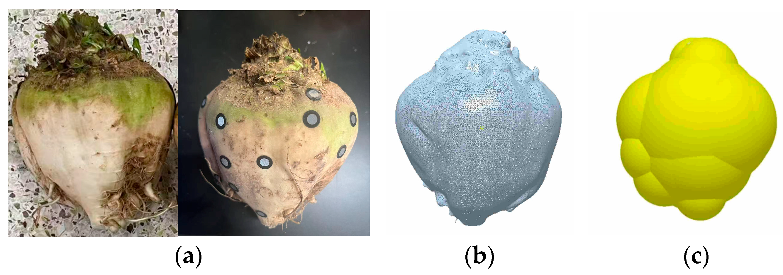
To improve the quality of the representative particle model, one sugar beet with a relatively intact shape and an overall contour closest to a sphere was selected from the 16 reconstructed samples as the representative sample for the discrete element modeling. This approach preserved the typical geometric characteristics of sugar beet roots while facilitating the subsequent approximation of the external contour using a multi-sphere agglomeration method. The reconstructed geometry was subsequently imported into EDEM2024 for automated particle filling, as shown in Figure 1.

2.1.2. Discrete Element Model

Sugar beet is a typical irregular block material. During digging operations, the friction, collision, and contact behaviors among materials are relatively complex, and a single-sphere model cannot accurately characterize the actual geometric features or mechanical response. Based on the contour model of the representative sugar beet root, the multi-sphere agglomeration method was adopted in this study to construct a discrete approximation [18]. After repeated model comparison and optimization, the final discrete element model of the sugar beet root consisted of 14 spherical elements, with a minimum sphere radius of 20 mm, a maximum sphere radius of 56 mm, and an average radius of 41.64 mm. The multi-sphere filling result for the sugar beet root is shown in Figure 1c.

2.2. Calibration of Contact Model Parameters

Agricultural materials often display strong anisotropic characteristics, and discrete element representations of irregular particles inherently deviate from real materials in both size and shape. As a result, discrepancies exist between simulated contact parameters and actual contact parameters, and the experimentally measured contact parameters cannot be directly applied to discrete element simulations [19,20]. In this work, the contact parameters used in the simulations were determined through a combination of bench-scale experiments and numerical analysis. Specifically, the contact parameters between the sugar beet and Q235 steel plates were calibrated. Commonly used calibration experiments for contact parameters include collision rebound, inclined plane sliding, inclined plane rolling, and piling experiments [21,22,23]. The data listed in

Table 1. Table of Physical Properties of Beets and Steel Plates.

Parameters	Value
Beet-to-Poisson ratio	0.4
Shear modulus of sugar beet/Pa	3 × 106
Beet density/(kg·m−3)	1100
Poisson’s ratio of Q235 steel	0.3
Shear modulus of Q235 steel/Pa	7.7 × 1010
Density of Q235 steel plate/(kg·m−3)	7850

were derived from the 2022 Science and Technology Achievement Transformation Project entitled “Key Technologies and Equipment for Sugar Beet Harvesting”.

2.2.1. Determination of Contact Parameters for Beet–Steel Interactions

Collision Recovery Coefficient

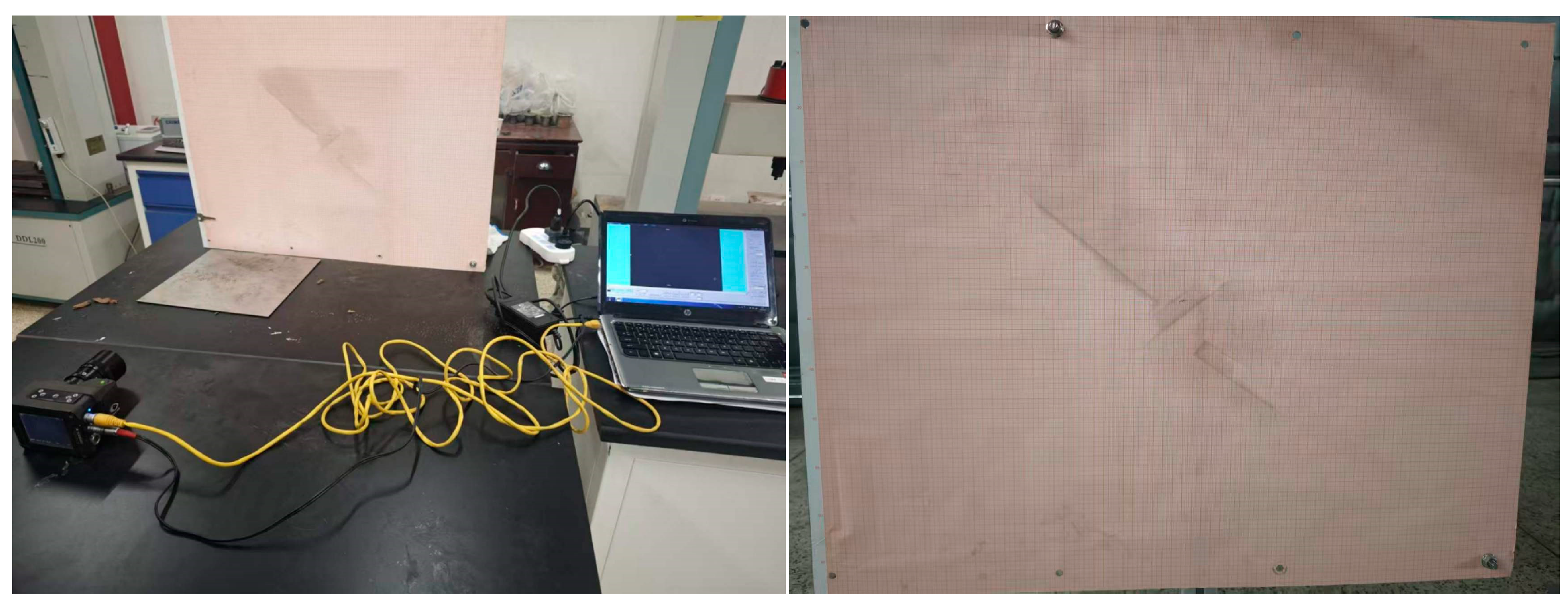
The restitution coefficient for the sugar beet–steel plate interface was obtained through a drop–rebound test [7]. The entire motion process was captured and recorded using a high-speed camera (MIRO eX2, Vision Research Inc., Wayne, NJ, USA), as shown in Figure 2.

The restitution coefficient e for the sugar beet particle–steel plate interaction was determined using the following expression:

$$e={\displaystyle \frac{v_1}{v_0}}={\displaystyle \frac{\sqrt{2g{H}_1}}{\sqrt{2g{H}_0}}}=\sqrt{{\displaystyle \frac{H_1}{H_0}}}$$

(1)

where $v_0$ is the velocity of the root immediately before contacting the impact surface, $v_1$ is the velocity of the root at the moment of rebound from the contact surface, $H_0$ is the initial release height of the root, and $H_1$ is the maximum rebound height of the root.

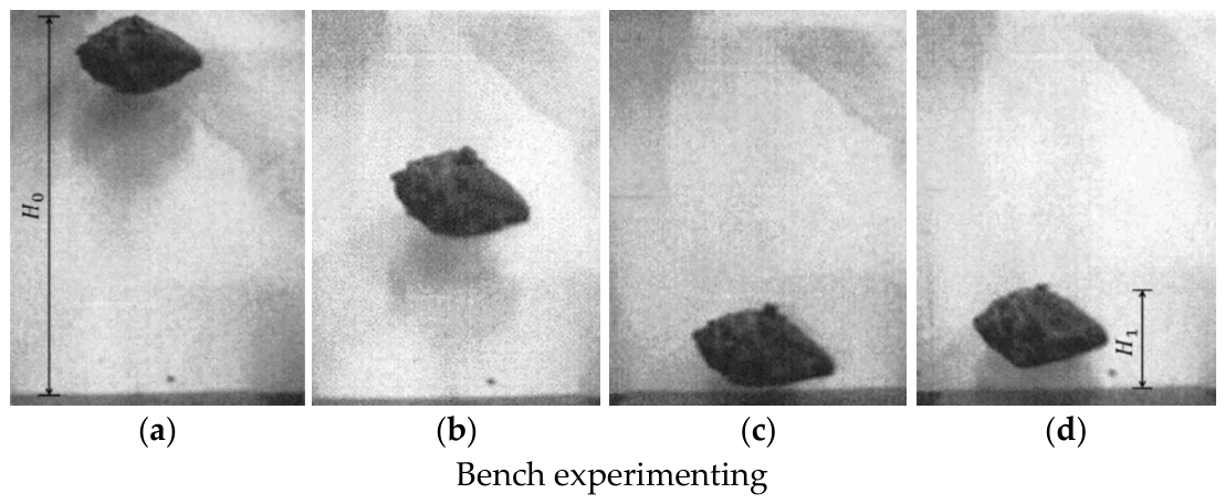
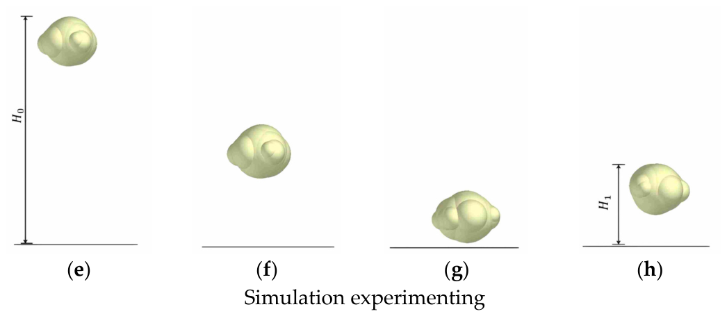
A sugar beet root was released from a preset height $H_0$ onto a horizontal steel plate. Its highest rebound position was recorded by a high-speed camera, and the rebound height $H_1$ was read from the coordinate grid. To improve the accuracy of the experimental results, three release heights, $H_0$ = 400, 450, and 500 mm, were selected, and 30 coefficient-of-restitution experiments were conducted at each height. The experimental procedure is illustrated in Figure 3. The measured average rebound heights, $H_1$, were (96.40 ± 40.43) mm, (108.84 ± 33.08) mm, and (118.60 ± 20.84) mm, respectively. In the simulation, 96.40, 108.84, and 118.60 mm were used as validation reference values. The corresponding coefficients of restitution, $e$, between the sugar beet and the steel plate were 0.491, 0.492, and 0.487, respectively. This indicated that changes in the initial release height had no significant effect on the coefficient of restitution. Therefore, an initial release height of ($H_0$ = 450) mm was selected for the simulation tests. Under this condition, the rebound height ($H_1$) ranged from 75.76 to 141.92 mm, and the coefficient of restitution $e$ calculated using Equation (1) ranged from 0.41 to 0.56.

In the simulation, the previously constructed sugar beet root model was used. The root was released from rest at a height of 450 mm above a horizontally positioned steel plate, allowing it to fall freely under gravity. The beet–steel restitution coefficient was varied within the range of 0.41–0.56, and the rebound height under each parameter setting was obtained using the EDEM2024 post-processing module. Based on the preliminary simulations, the final simulation scheme and corresponding results were determined.

Coefficient of Static Friction

The static friction coefficient was obtained using an inclined-plane sliding test [24]. The static friction coefficient ${\mu }_s$ is related to the inclination angle $\alpha$ as follows:

$${\mu }_s={\displaystyle \frac{f}{T}}={\displaystyle \frac{\mathrm{mg}\sin \alpha }{\mathrm{mg}\cos \alpha }}=\tan \alpha$$

(2)

where $f$ denotes the frictional force, $T$ is the normal reaction of the inclined surface acting on the sugar beet root, and $\alpha$ represents the tilt angle of the steel plate relative to the horizontal direction.

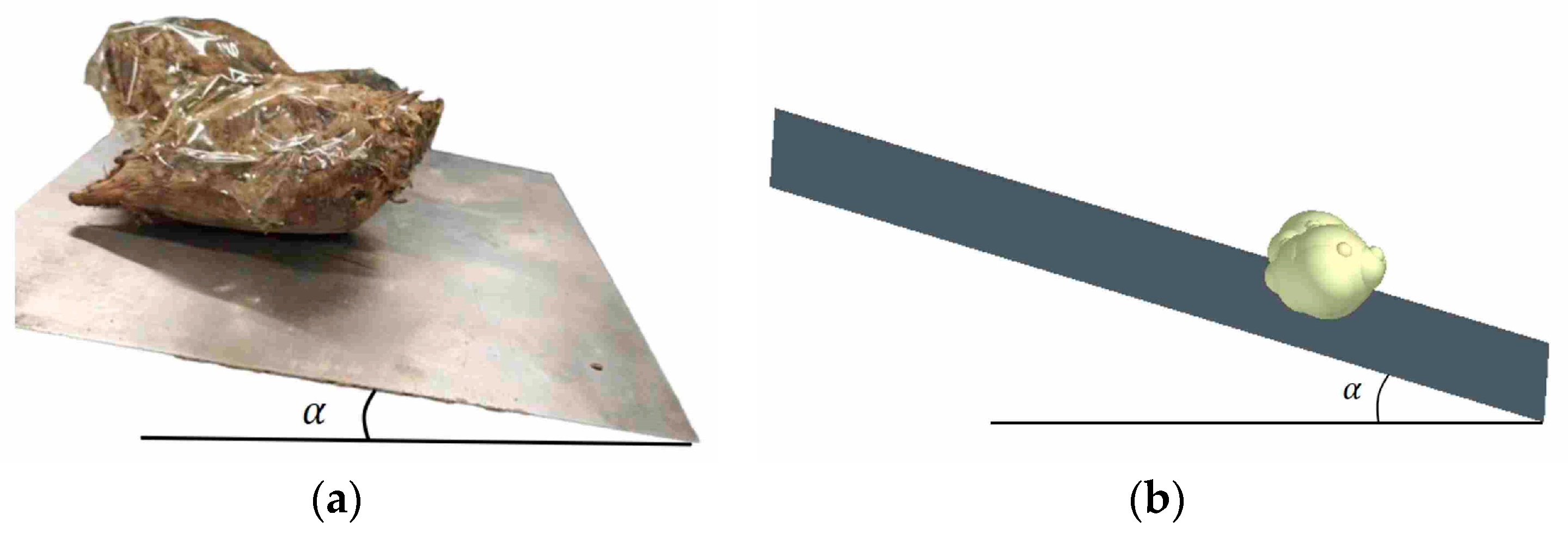
The inclined-plane test was conducted using a Q235 steel plate, as illustrated in Figure 4. Two oval-shaped sugar beet roots were bonded together before testing to minimize rolling and ensure sliding-dominated motion. During the test, the plate was gradually raised from one end while the other end remained fixed on the horizontal bench. The inclination angle at the onset of sliding was measured with a digital angle gauge with an accuracy of 0.05° and a measurement range of 0–360°. After 30 repeated tests, the mean critical sliding angle was $\alpha$ = 37.14 ± 6.14°, corresponding to a sugar beet–steel plate static friction coefficient of ${\mu }_s$ = 0.757 ± 0.157. This angle was subsequently used as the reference value for the simulation.

In EDEM2024, the inclined-plane sliding model was built using a 300 mm × 300 mm square plate assigned with the material properties of Q235 steel. Two sugar beet roots were bonded into a single unit to avoid rolling during sliding. To isolate the influence of static friction, the restitution coefficient was held at its calibrated value of 0.517, while the rolling friction coefficient was set to zero. The sugar beet–steel plate static friction coefficient, $x_2$, was then varied from 0.55 to 0.95. Seven simulation cases were carried out, with five repetitions for each case, and the mean values were used in the analysis.

Coefficient of Rolling Friction

The rolling friction coefficient was determined using an inclined-plane rolling test [25]. Based on the principle of energy conservation:

$$mgS\sin \beta ={\mu }_{r}mg\left(S\cos \beta +L\right)$$

(3)

Thus, the rolling friction coefficient ${\mu }_r$ can be derived as:

$${\mu }_r={\displaystyle \frac{S\sin \beta }{S\cos \beta +L}}$$

(4)

where $\beta$ denotes the tilt angle of the steel plate, while $S$ and $L$ correspond to the rolling distances of the sugar beet root along the inclined section and on the horizontal steel plate, respectively.

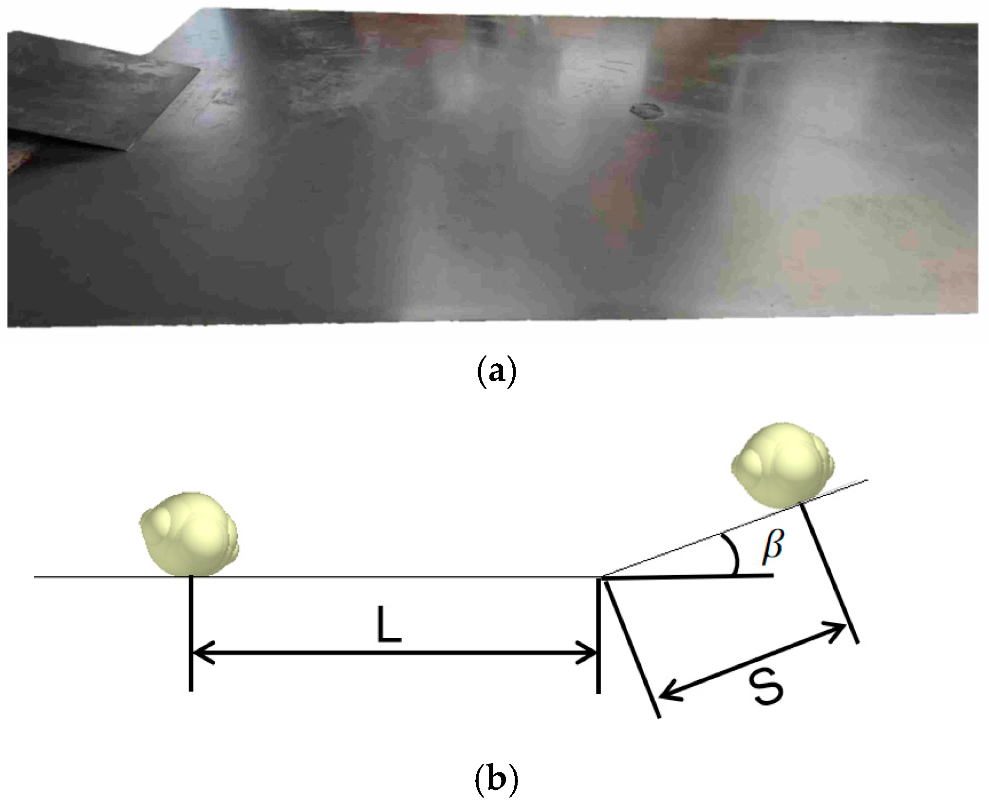
The experiment bench was composed of two steel plates, as shown in Figure 5. Preliminary tests showed that when the inclination angle was too large, the sugar beet root might bounce after rolling onto the horizontal plate, leading to measurement errors; when the inclination angle was too small, the root might stop before completing the rolling process, the inclination angle of the steel plate was set to $\beta$ = 20° and the rolling distance of the sugar beet root on the inclined plane was set to $S$ = 300 mm. Following the inclined-plane rolling test procedure, 30 repeated measurements were performed, giving an average horizontal rolling distance of $L$ = 656.3 ± 69.6 mm. By substituting the measured values into Equation (4), the sugar beet–steel rolling friction coefficient under the experimental conditions was calculated as ${\mu }_r$ = 0.11.

For the rolling simulation, an inclined–horizontal plate system was constructed in EDEM2024. One rectangular plate was inclined at (20°), and its lower end was connected to a horizontal rectangular plate. Both plates were assigned the material properties of Q235 steel. A sugar beet root was positioned on the inclined plate at a distance of ($S$ = 300) mm from the lower end and released from rest to roll down the slope. The calibrated sugar beet–steel restitution coefficient and static friction coefficient were fixed at ($e$ = 0.517) and (${\mu }_s$ = 0.757), respectively. The rolling friction coefficient was then varied from 0.09 to 0.13. Seven simulation cases were conducted, each with five repetitions, and the mean values were used as the final results.

2.2.2. Determination of Contact Parameters for Sugar Beet–Sugar Beet Interactions

The angle of repose is a macroscopic indicator commonly used to characterize material flowability and frictional behavior. Among the contact parameters, the static and rolling friction coefficients have a pronounced influence on this response. After calibrating the sugar beet–steel plate parameters described above, the inter-root contact parameters of sugar beet roots were further analyzed and calibrated. Specifically, the steepest-ascent test and the quadratic orthogonal rotatable regression design were used to determine the static friction coefficient, rolling friction coefficient, and other relevant simulation parameters between sugar beet roots.

Pile-Up Experiment

To determine the angle of repose of sugar beet roots, image processing and geometric parameter extraction were performed based on the side-view image of the pile. The original color image of the pile was first captured using a camera mounted on a fixed tripod. Before image acquisition, the tripod was adjusted with a spirit level to ensure that the camera remained horizontally aligned, and the optical axis of the camera was kept perpendicular to the pile profile. The camera height was adjusted to be approximately level with the central height of the pile to reduce geometric distortion during image capture. The image was then imported into MATLAB2007 and converted into a grayscale image. Threshold segmentation was subsequently applied to obtain a binary image, from which the surface boundary of the pile was extracted. Based on the extracted boundary, the contour points located on the stable inclined surface of the pile were selected, and linear fitting was performed for the selected boundary points. The angle of repose was calculated from the slope of the fitted line.

In the DEM analysis, the simulated repose angle was obtained by adopting the cylinder-lifting procedure. During this stage, the calibrated contact parameters for the sugar beet root–steel plate interaction were held constant. The restitution coefficient, static friction coefficient, and rolling friction coefficient between sugar beet roots were treated as the three variables to be optimized. The agreement between the DEM simulation and the bench-scale piling test was evaluated using the deviation between the simulated and measured repose angles. Accordingly, the relative error, $\delta$, was selected as the response index and was calculated as follows:

$$\delta ={\displaystyle \frac{|{\theta }^{\prime }-\theta |}{\theta }}\times 100$$

(5)

where ${\theta }^{\prime }$ represents the simulated angle of repose, and $\theta$ represents the measured angle of repose.

Steepest Climb Experiment

To rapidly determine the reasonable ranges of the contact parameters between sugar beet roots, the steepest ascent method was employed. In this method, the parameter combination is progressively adjusted in the direction of the most rapid change in the relative error of the angle of repose within the multi-factor parameter space, so as to narrow the search range for the optimal parameters. Based on preliminary simulations, the factor ranges were determined.

Quadratic Orthogonal Rotatable Regression Experiment

To obtain the optimal contact parameters for root–root interactions in the EDEM2024 model, a quadratic orthogonal rotatable regression scheme involving three variables was employed. The restitution coefficient, static friction coefficient, and rolling friction coefficient between sugar beet roots were taken as the independent variables. The response index was defined as the relative error between the DEM-predicted angle of repose and the experimentally measured value.

3. Results

3.1. Restitution Coefficient Calibration and Result Analysis

The simulated collision–rebound results for the sugar beet root–steel plate contact are summarized in

Table 2. Simulation Experiment Results for the Rebound Coefficient of Beet-Steel Plate Collisions.

NO	Recovery Factor ${\mathit{x}}_1$	Rebound Height ${\mathit{y}}_1$/mm
1	0.41	82.15
2	0.45	88.59
3	0.49	99.44
4	0.53	123.97
5	0.56	126.25

. In this table, $x_1$ refers to the restitution coefficient, whereas $y_1$ represents the rebound height.

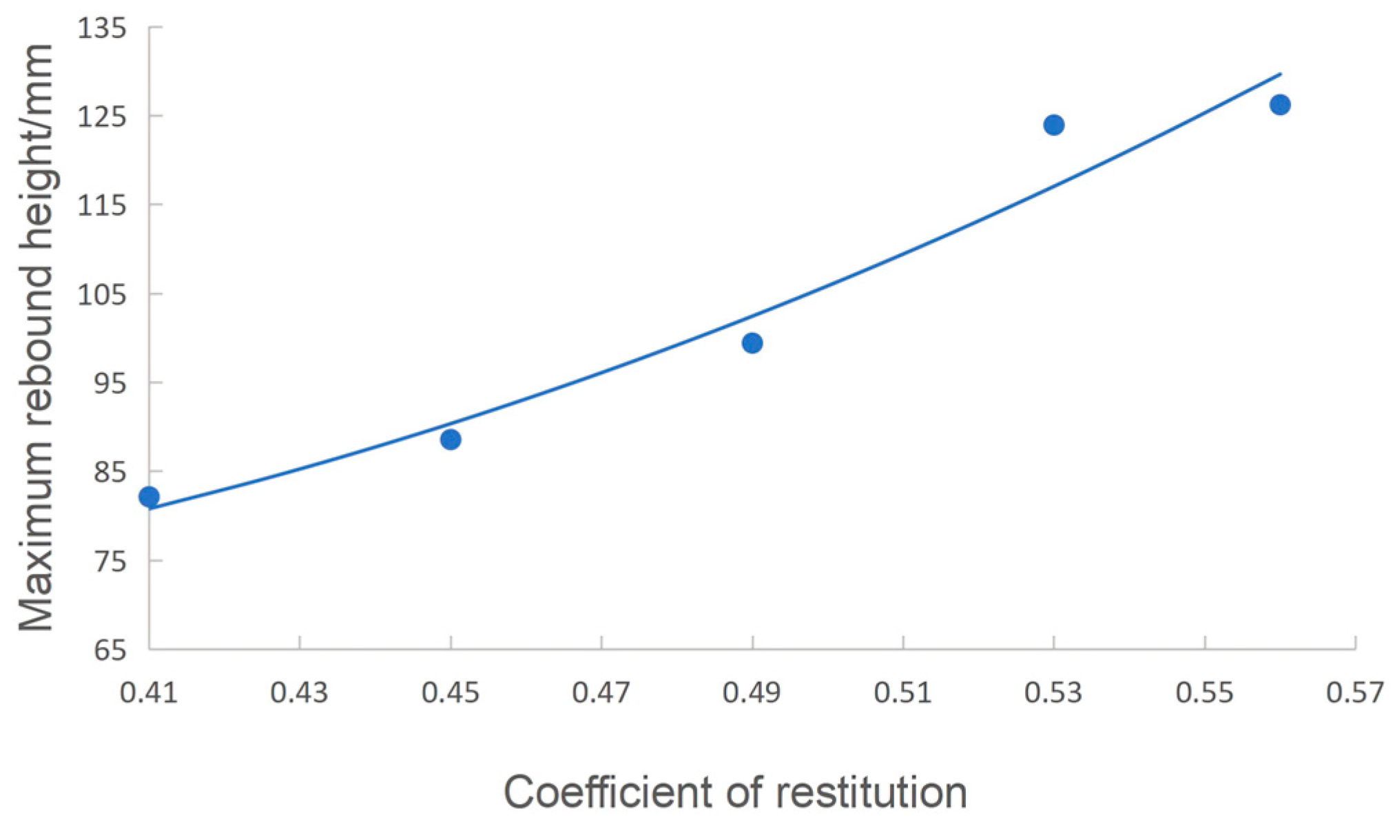
By fitting the data in Table 2, a quadratic polynomial relationship was obtained, as illustrated in Figure 6, and the corresponding equation is given as follows:

$$y_1=785.83x_1^2-436.44x_1+127.65$$

(6)

The fitted equation had a high coefficient of determination $R^2$ = 0.9549, indicating that it effectively described the relationship between rebound height and the coefficient of restitution for the sugar beet–steel plate contact. Substituting $y_1$ = 108.84 mm into fitting Equation (6) yielded $x_1$ = 0.508. This value was then used as the restitution coefficient in the validation simulations at $H_0$ = 400, 450, and 500 mm, with three replicates for each condition. The mean simulated rebound heights, $H_1^{\prime }$, were 95.76, 106.78, and 116.43 mm. The corresponding relative errors were 0.66%, 1.89%, and 1.83%, confirming good consistency between the simulated and experimental rebound heights. Thus, the coefficient of restitution for the sugar beet–steel plate contact was determined as 0.508 for subsequent EDEM simulations.

3.2. Static Friction Coefficient: Calibration Results and Analysis

The simulation results for the static friction coefficient are shown in

Table 3. Results of Simulation Experiments on the Static Coefficient of Friction.

NO	Static Friction Coefficient ${\mathit{x}}_2$	Angle of Inclination ${\mathit{y}}_2$/°
1	0.55	28.84
2	0.62	31.80
3	0.69	34.66
4	0.76	37.28
5	0.83	39.69
6	0.90	42.00
7	0.95	43.55

, where $x_2$ denotes the static friction coefficient and $y_2$ denotes the simulated inclination angle of the inclined plate.

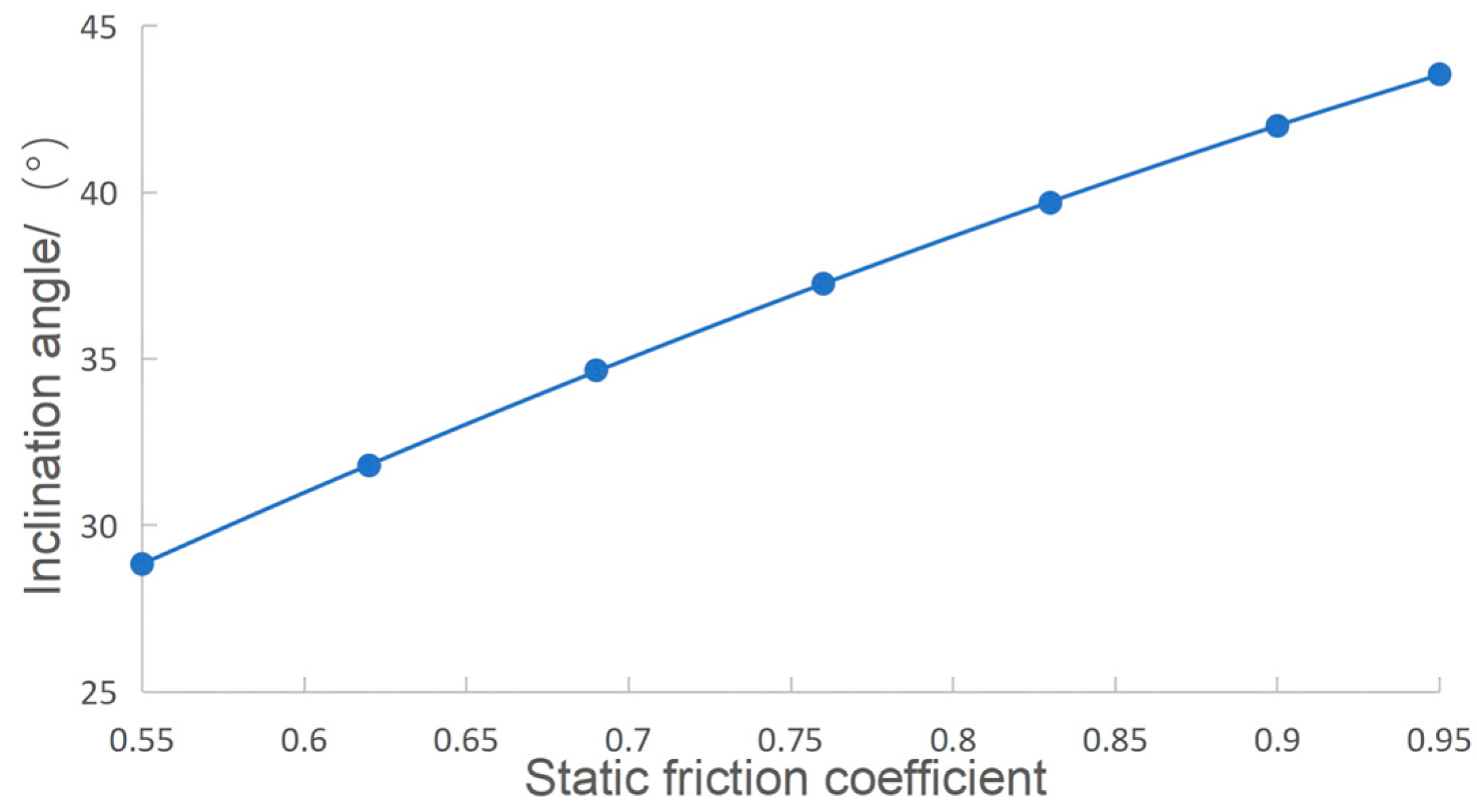
A quadratic polynomial was fitted to the experimental data, as depicted in Figure 7, and the resulting relationship is expressed as:

$$y_2=-17.556x_2^2+63.072x_2-0.5376$$

(7)

The regression yielded a determination coefficient of ($R^2$ = 1), demonstrating a perfect correspondence between the sugar beet–steel static friction coefficient and the plane inclination angle. Substituting $y_2$ = 37.14° into fitting Equation (7) gave $x_2$ = 0.757. This value was then used in three validation simulations, which produced plate inclination angles of 37.11°, 37.23°, and 37.12°. The mean simulated angle was 37.15°, differing from the experimental value by only 0.03%. The close agreement confirms the reliability of the calibrated parameter. Therefore, the static friction coefficient for the sugar beet–steel plate contact was set as ${\mu }_s$ = 0.757 in the EDEM simulation.

3.3. Calibration Results and Analysis of the Rolling Friction Coefficient

The simulated data for rolling friction calibration are summarized in

Table 4. Results of Simulation Experiments on the Coefficient of Kinetic Friction.

NO	Rolling Friction Coefficient ${\mathit{x}}_3$	Scroll Distance ${\mathit{y}}_3$/mm
1	0.090	752.6
2	0.097	682.5
3	0.103	612.1
4	0.110	562.7
5	0.117	512.2
6	0.123	472.3
7	0.130	432.9

. Here, $x_3$ refers to the rolling friction coefficient, and $y_3$ indicates the corresponding rolling distance.

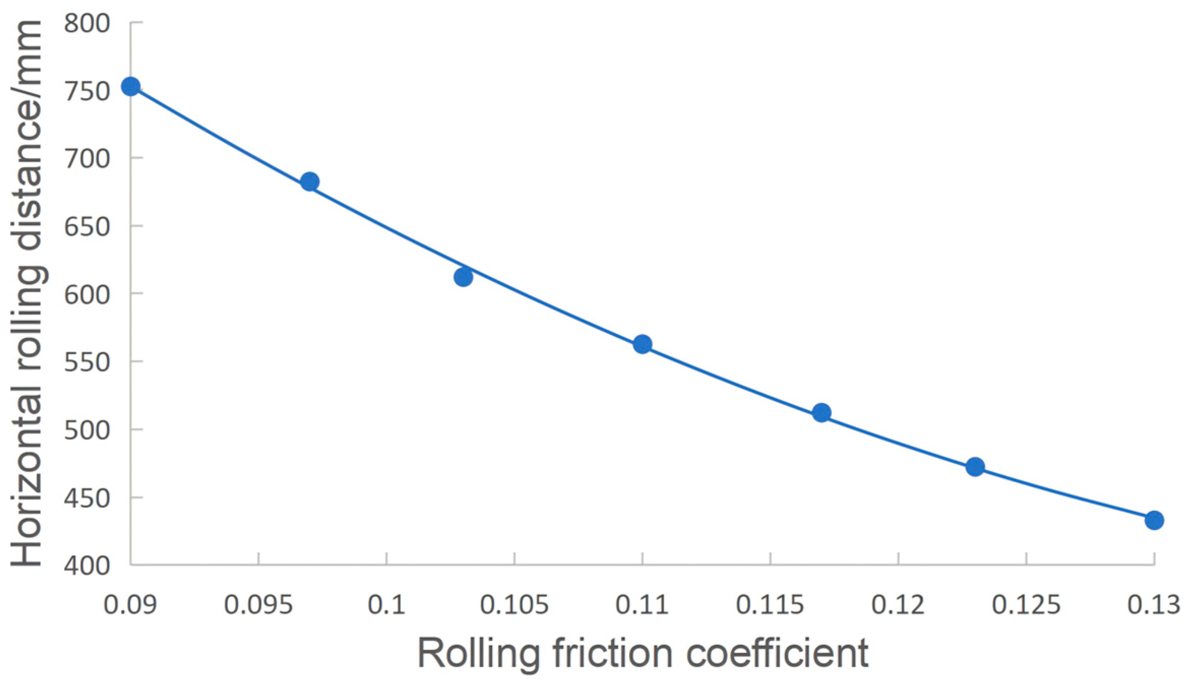
Taking the rolling friction coefficient $x_3$ as the independent variable and the rolling distance on the horizontal plate $L$ as the response, the data were fitted to obtain the relationship shown in Figure 8, from which the following equation was derived:

$$y_3=81535x_3^2-25887x_3+2422$$

(8)

The coefficient of determination of the fitted regression equation was $R^2$ = 0.9987, indicating that the equation could reliably describe the relationship between the simulated rolling friction coefficient $x_3$ and the horizontal rolling distance $y_3$. In this study, the experimentally measured average horizontal rolling distance $L$ = 656.3 ± 69.6 mm was used as the target value for calibration. Therefore, $y_3$ in Equation (8) was set equal to the measured value $L$, and the corresponding rolling friction coefficient was obtained by solving the regression equation. The calculated value was $x_3$ = 0.099. To verify this calibrated value, five repeated inclined-plane rolling simulations were conducted using $x_3$ = 0.099. The simulated rolling distances were 652.6, 644.1, 645.9, 645.5, and 655.7 mm, with an average value of 648.76 mm. The relative error between the simulated average rolling distance and the measured value was 1.15%, indicating that the calibrated rolling friction coefficient was consistent with the experimental result. Therefore, the sugar beet–steel rolling friction coefficient used in the EDEM simulation was set to ${\mu }_r$ = 0.099.

3.4. Result Analysis of Inter-Root Contact Parameter Calibration

3.4.1. Analysis of the Results of the Stacking Experiment

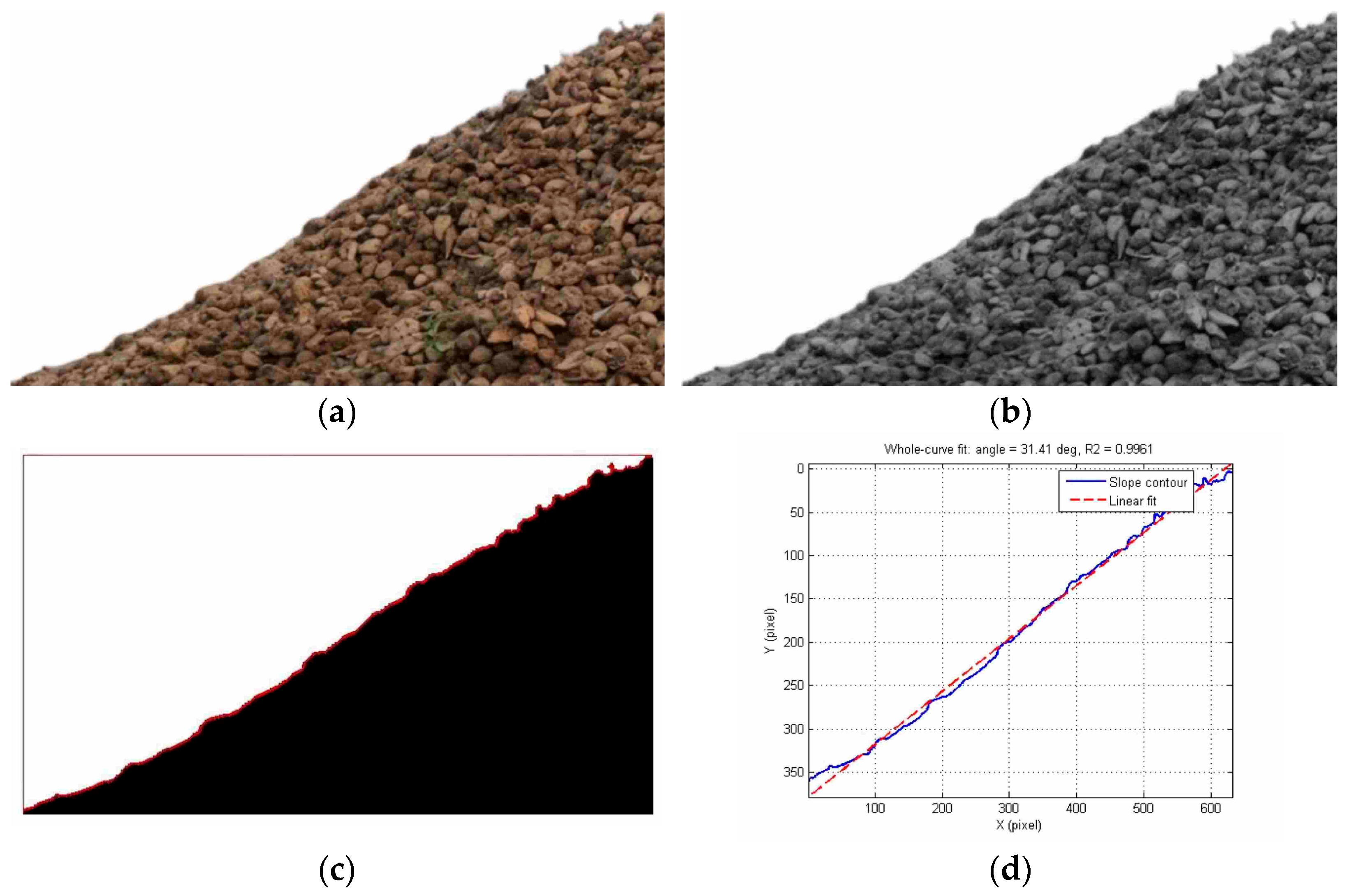
To accurately determine the angle of repose of sugar beet roots, image processing and geometric parameter extraction were performed for the piling test. First, the original color image of the pile from the side view was captured using a camera, as shown in Figure 9a. The image was then imported into MATLAB and converted into a grayscale image, as shown in Figure 9b. After grayscale processing, threshold segmentation was applied to obtain a binary image, and the surface boundary profile of the pile was extracted, as shown in Figure 9c. Based on the extracted boundary, the contour points located on the inclined surface of the pile were screened, and the boundary points within the valid region were selected for linear fitting, as shown in Figure 9d. The angle of repose was then calculated from the slope of the fitted line, giving a measured value of $\theta$ = 31.41°.

3.4.2. Analysis of the Results from the Steepest Climb Experiment

The results of the steepest climb experiment are presented in

Table 5. Results of the Steepest Climb Experiment.

NO	Experimental Factors			Experiment Results
	e	μs	μr	Simulated Value (°)	Measured Values (°)	Relative Error (%)
a	0.40	0.60	0.05	27.03	31.41	13.94
b	0.45	0.65	0.06	29.35	31.41	6.56
c	0.50	0.70	0.07	30.31	31.41	3.50
d	0.55	0.75	0.08	31.14	31.41	0.86
e	0.60	0.80	0.09	32.23	31.41	2.61
f	0.65	0.85	0.10	35.17	31.41	11.97
g	0.70	0.90	0.11	37.37	31.41	18.97

.

As presented in Table 5, the relative error of the angle of repose exhibited a decreasing–increasing trend. The lowest error occurred in group d, suggesting that the optimal parameter range is centered around this condition. Therefore, the factor combinations of groups c, d, and e were selected as the −1, 0, and 1 levels, respectively, for the subsequent quadratic orthogonal rotatable regression design.

3.4.3. Analysis of Quadratic Orthogonal Rotatable Regression Results

The coding scheme for the simulation factors is shown in

Table 6. Simulation Experiment Code Table.

Coding	Factors
	$\mathit{e}$	μs	μr
$-1.682$	0.466	0.666	0.063
$-1$	0.50	0.70	0.07
$0$	0.55	0.75	0.08
$1$	0.60	0.80	0.09
1.682	0.634	0.834	0.097

, and the results of the quadratic orthogonal rotatable regression design are presented in

Table 7. Experiment Protocol and Results.

$\mathbf{NO}$	Experimental Factors			Y/%
	$\mathbf{A}$	$\mathbf{B}$	$\mathbf{C}$
1	−1	−1	−1	1.97
2	1	−1	−1	6.14
3	−1	1	−1	7.26
4	1	1	−1	12.51
5	−1	−1	1	0.25
6	1	−1	1	6.14
7	−1	1	1	12.38
8	1	1	1	18.34
9	−1.682	0	0	0.89
10	1.682	0	0	12.16
11	0	−1.682	0	0.8
12	0	1.682	0	12.77
13	0	0	−1.682	2.2
14	0	0	1.682	11.56
15	0	0	0	3.62
16	0	0	0	0.86
17	0	0	0	3.92
18	0	0	0	0.8
19	0	0	0	1.66
20	0	0	0	0.38
21	0	0	0	4.04
22	0	0	0	0.92
23	0	0	0	0.19

. In Table 7, the experimental factors A, B, and C represent the coefficient of restitution, static friction coefficient, and rolling friction coefficient, respectively.

The experimental data were subjected to multiple regression analysis using Design-Expert 13.0, and the regression model describing the relative error $Y$ of the angle of repose was established as follows:

$$Y=1.80+2.95A+4.11B+1.83C+0.14AB+0.3AC+1.58BC+1.89A^2+1.98B^2+2.02C^2$$

(9)

The significance of the fitted regression model was examined, with the analysis results summarized in

Table 8. ANOVA Results for the Regression Model.

Sources of Variance	$\mathbf{S}\mathbf{u}\mathbf{m}\hspace{0.33em}\mathbf{o}\mathbf{f}\hspace{0.33em}\mathbf{S}\mathbf{q}\mathbf{u}\mathbf{a}\mathbf{r}\mathbf{e}\mathbf{s}$	$\mathbf{D}\mathbf{e}\mathbf{g}\mathbf{r}\mathbf{e}\mathbf{e}\mathbf{s}\hspace{0.33em}\mathbf{o}\mathbf{f}\hspace{0.33em}\mathbf{F}\mathbf{r}\mathbf{e}\mathbf{e}\mathbf{d}\mathbf{o}\mathbf{m}$	$\mathit{F}$	$\mathit{p}$	$\mathbf{S}\mathbf{i}\mathbf{g}\mathbf{n}\mathbf{i}\mathbf{f}\mathbf{i}\mathbf{c}\mathbf{a}\mathbf{n}\mathbf{c}\mathbf{e}$
Model	597	9	23.07	<0.0001	**
A	118.47	1	41.20	<0.0001	**
B	230.62	1	80.20	<0.0001	**
C	45.66	1	15.88	0.0016	**
AB	0.1653	1	0.0575	0.8142
AC	0.7381	1	0.2567	0.6209
BC	20.07	1	6.98	0.0203	*
A2	56.78	1	19.75	0.0007	**
B2	62.43	1	21.71	0.0004	**
C2	64.57	1	22.46	0.0004	**
Residual	37.38	13
Analogy	17.27	5	1.37	0.3276
Error	20.11	8
Total	634.38	22

Note: * denotes statistical significance (p < 0.05), ** denotes high statistical significance (p < 0.01).

. The overall model reached a highly significant level (p < 0.01), demonstrating that the established model fitted the response well. For the interaction effects, AB and AC, representing the restitution coefficient–static friction coefficient interaction and the restitution coefficient–rolling friction coefficient interaction, respectively, were not statistically significant (p > 0.1). In contrast, the remaining model terms exerted significant influences on the relative error of the angle of repose. This indicates that the response was mainly affected by nonlinear and quadratic effects rather than a simple linear relationship. Moreover, the lack-of-fit test was not significant (p = 0.3276), suggesting that the model adequately described the experimental data and that no obvious systematic factors were omitted. The regression equation yielded a determination coefficient of ($R^2$ = 0.94), showing good agreement between the predicted and observed values.

3.4.4. Response Surface Analysis

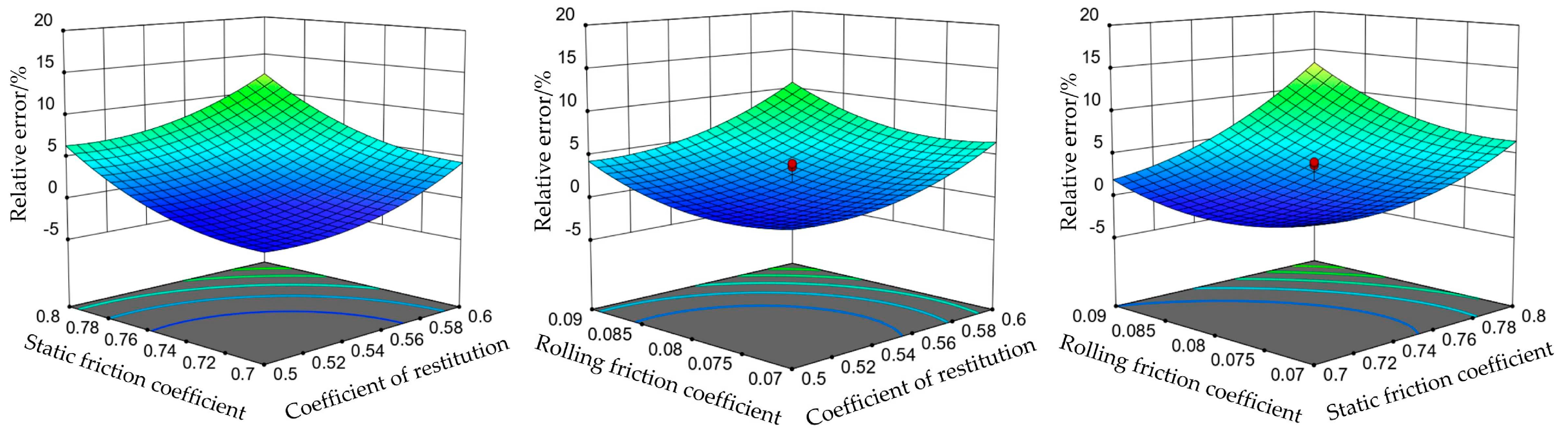
Figure 10 illustrates the response surface plots obtained from the regression analysis. The plots show that the three inter-root contact parameters contributed differently to the variation in the repose-angle error. Among these factors, the static friction coefficient produced the strongest influence on the response, followed by the restitution coefficient and the rolling friction coefficient. The curved trends observed in the response surfaces indicate that the effects of the factors were nonlinear rather than purely linear. In addition, interaction effects were present between some factors, but their influence was generally weaker than that of the individual factors. Overall, the influence of the inter-root contact parameters on the repose-angle error decreased in the following order: static friction coefficient > restitution coefficient > rolling friction coefficient.

3.4.5. Optimal Parameters

The fitted regression equation was solved in Design-Expert 13.0, with the minimization of the relative error in the angle of repose taken as the optimization criterion. Based on the response surface analysis, the optimal combination of contact parameters was then obtained. The optimization target and corresponding constraints were specified as follows:

$$\left\{\begin{array}{l}\min Y\left(X_1,X_2,X_3\right)\hfill \\ s.t.\left\{\begin{array}{l}0.466\le X_1\le 0.634\hfill \\ 0.666\le X_2\le 0.834\hfill \\ 0.063\le X_3\le 0.097\hfill \end{array}\right.\hfill \end{array}\right.$$

(10)

The optimization produced multiple feasible parameter combinations, and the final inter-root restitution, static friction, and rolling friction coefficients were determined as 0.534, 0.728, and 0.080, respectively. These values were applied in EDEM2024 for three repeated angle-of-repose simulations, producing results of 31.33°, 31.14°, and 30.96°, with a mean value of 31.14°. Compared with the measured angle of repose, the mean simulated value showed a relative error of only 0.86%. This low deviation verifies the reliability of the calibrated parameters and supports their use in subsequent DEM simulations of sugar beet roots.

3.4.6. Validation Experiment

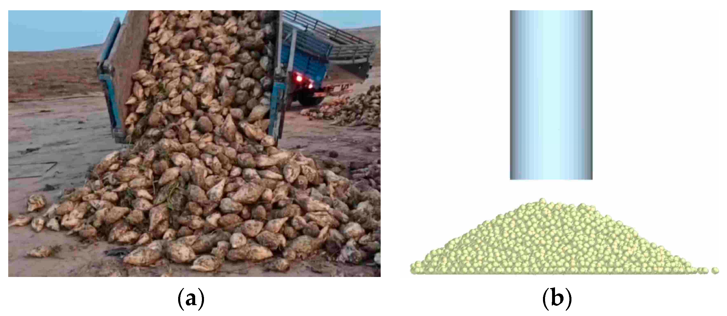
To verify the applicability of the calibrated DEM model under unloading conditions, a field piling test was performed using natural discharge from a transport vehicle. Sugar beets were released from a certain height and accumulated under gravity into a stable pile, as shown in Figure 11. Image analysis gave a measured angle of repose of 31.76°. In the corresponding EDEM simulation, the calibrated sugar beet root contact parameters were applied, and a cylindrical container was used to reproduce the vehicle unloading process. After release from a fixed height, the simulated roots formed a pile under gravity. Three repeated simulations produced repose angles of 31.17°, 32.15°, and 33.37°, with a mean of 32.23°. The difference from the field measurement was 1.5%, indicating that the developed model and calibrated parameters can reliably describe the piling behavior of sugar beet roots under unloading conditions.

4. Discussion

Previous studies have established a relatively clear workflow for DEM calibration of agricultural particles, namely geometric modeling, contact parameter calibration, and macroscopic validation [26]. For sunflower seeds, the inter-particle static and rolling friction coefficients were identified as important parameters affecting the angle of repose, and the calibrated model was verified with relative errors of 1.43% and 0.40% for two sunflower varieties [27]. In the calibration of coated maize particles, the inter-particle static and rolling friction coefficients, together with the particle–wall rolling friction coefficient, were found to significantly influence the angle of repose, and the optimized parameter set produced a validation error of only 0.22% [28]. Similarly, for pod pepper seeds, a reverse-engineering-based DEM model combined with response surface optimization was established, and the calibrated parameters were verified by cylinder-lifting and plate-drawing tests, with relative errors of 1.524% and 2.975%, respectively [29]. Compared with these studies, the present work focused on sugar beet roots, which are much larger and more irregular than seed particles and have more complex geometric and mass-distribution characteristics. After calibration, the relative error between the simulated and measured angles of repose was 0.86%, and the error in the independent unloading validation test was 1.5%. These values are comparable to those reported for seed and small-particle materials, indicating that the proposed parameter calibration procedure can effectively reproduce the macroscopic piling behavior of large irregular sugar beet roots. Therefore, the combined use of three-dimensional scanning, multi-sphere clump modeling, contact parameter calibration, and repose-angle validation provides a feasible DEM modeling strategy for irregular root crop materials.

Nevertheless, several limitations remain in the present study. First, the multi-sphere clump model is still an approximation of the real beet geometry and cannot fully capture surface roughness, local protrusions and depressions, or heterogeneous mass distribution. Second, although the repose angle is highly sensitive to static and rolling friction, its sensitivity to restitution is relatively limited, which means that some degree of equivalent parameter compensation may still exist during inverse calibration. In addition, the validation scenarios in this study mainly focused on piling and natural unloading processes, whereas more complex engineering conditions such as conveying and digging have not yet been considered. Future work should therefore improve the geometric fidelity of the DEM model, introduce multi-response calibration strategies by combining rolling distance, critical sliding angle, and dynamic response indicators, and further extend validation to component-level operating conditions in sugar beet harvesting and transport equipment, thereby enhancing the generalizability and engineering applicability of the calibrated parameter system.

5. Conclusions

(1) In this study, sugar beet roots were represented in the DEM environment through a workflow combining 3D scanning, reverse reconstruction, and multi-sphere clump generation. The resulting particle representation consisted of 14 spherical elements and was introduced into EDEM2024 with the Hertz–Mindlin no-slip contact law, thereby providing the geometric representation and contact-mechanics basis required for subsequent parameter calibration.

(2) For the interaction between sugar beet roots and Q235 steel, the required contact parameters were determined by combining EDEM simulations with drop-impact, slope-sliding, and slope-rolling bench tests. The obtained restitution, static friction, and rolling friction coefficients for the beet–steel contact were 0.508, 0.757, and 0.099, respectively. The verification results showed good agreement between the simulated responses and the measured data, indicating that these calibrated parameters can reasonably describe the rebound, sliding, and rolling characteristics of sugar beet roots on steel plates.

(3) For the calibration of beet–beet contact parameters, the repose angle was selected as the target response. A steepest-ascent procedure was first used to narrow the parameter range, followed by a quadratic orthogonal rotatable regression design to further optimize the inter-root parameters. The calibrated beet–beet restitution coefficient, static friction coefficient, and rolling friction coefficient were 0.534, 0.728, and 0.080, respectively. When these parameters were applied in the DEM simulation, the predicted repose angle showed a relative deviation of only 0.86% from the experimental value. In addition, the independent natural unloading validation test gave a relative error of 1.5%. These results demonstrate that the developed DEM model and calibrated parameter set can effectively characterize the piling behavior of sugar beet roots and provide useful parameter support for simulations related to sugar beet handling, transportation, and equipment optimization.

References

- Rahenbrock, D.; Varrelmann, M. Comparative small RNA profiles of beet mosaic virus (BtMV), beet mild yellowing virus (BMYV) and beet yellows virus (BYV) infected Nicotiana benthamiana and Beta vulgaris. Virus Res. 2025, 361, 199640. [Google Scholar] [CrossRef] [Scilit] [PubMed]
- Großmann, F. What drives yield formation in sugar beet? Quantifying functional components across genotypes and irrigation managements. Field Crops Res. 2026, 338, 110292. [Google Scholar] [CrossRef] [Scilit]
- Yang, L. Discrete element contact model and parameter calibration for clayey soil particles in the Southwest hill and mountain region. J. Terramech. 2024, 111, 73–87. [Google Scholar] [CrossRef] [Scilit]
- Zhao, J. Modelling method and test verification of wheat plants with leaves for discrete element simulation of the harvesting process. Biosyst. Eng. 2026, 265, 104436. [Google Scholar] [CrossRef] [Scilit]
- Chen, Z. Coefficient of restitution considerations in the discrete element method for agricultural materials: A review. Biosyst. Eng. 2026, 262, 104364. [Google Scholar] [CrossRef] [Scilit]
- Wu, Z. Calibration of discrete element parameters and experimental verification for modelling subsurface soils. Biosyst. Eng. 2021, 212, 215–227. [Google Scholar] [CrossRef] [Scilit]
- Zheng, G. Calibration and testing of discrete element simulation parameters for spinach seeds. Comput. Part. Mech. 2025, 12, 479–490. [Google Scholar] [CrossRef] [Scilit]
- Zhu, Y. Discrete element modelling and parameter calibration method for a flexible wheat plant with breakable grains. Biosyst. Eng. 2026, 264, 104405. [Google Scholar] [CrossRef] [Scilit]
- Fan, J. A general discrete element modelling method and harvest process for wheat plants. Biosyst. Eng. 2025, 259, 104284. [Google Scholar] [CrossRef] [Scilit]
- Horabik, J.; Molenda, M. Parameters and contact models for DEM simulations of agricultural granular materials: A review. Biosyst. Eng. 2016, 147, 206–225. [Google Scholar] [CrossRef] [Scilit]
- Fan, J. Experimental verification and simulation analysis of a multi-sphere modelling approach for wheat seed particles based on the discrete element method. Biosyst. Eng. 2024, 245, 135–151. [Google Scholar] [CrossRef] [Scilit]
- Guo, H. Design and simulation of a garlic seed metering mechanism. Agriculture 2021, 11, 1239. [Google Scholar] [CrossRef] [Scilit]
- Dong, X.Q.; Zheng, H.N.; Jia, X. Calibration and experiments of the discrete element simulation parameters for rice bud damage. INMATEH Agric. Eng. 2022, 68, 659–668. [Google Scholar] [CrossRef] [Scilit]
- Yang, L. Parameter calibration for discrete element simulation of Leymus chinensis seeds based on RSM optimization. Sci. Rep. 2025, 15, 7947. [Google Scholar] [CrossRef] [Scilit] [PubMed]
- Bai, H.; Liu, F.; Dong, W. DEM modelling methods and trait analysis of sunflower seed. Biosyst. Eng. 2025, 250, 39–48. [Google Scholar] [CrossRef] [Scilit]
- Shi, L. Modeling of typically shaped corn seeds and calibration of the coefficient of rolling friction. Agronomy 2023, 13, 1573. [Google Scholar] [CrossRef] [Scilit]
- Chen, K. Contact parameter calibration for discrete element potato minituber seed simulation. Agriculture 2024, 14, 2298. [Google Scholar] [CrossRef] [Scilit]
- Zhang, S. DEM contact parameters of rice seed for mechanical seeding performance analysis. Biosyst. Eng. 2025, 260, 104298. [Google Scholar] [CrossRef] [Scilit]
- Liu, Y.; Liu, H.; Mao, H. The influence of rolling resistance on the stress-dilatancy and fabric anisotropy of granular materials. Granul. Matter 2018, 20, 12. [Google Scholar] [CrossRef] [Scilit]
- Kim, B.-S. Effects of grain shape on mechanical behavior of granular materials using DEM analysis. KSCE J. Civ. Eng. 2021, 25, 1939–1950. [Google Scholar] [CrossRef] [Scilit]
- Du, C. Calibration of contact parameters for complex shaped fruits based on discrete element method: The case of pod pepper (Capsicum annuum). Biosyst. Eng. 2023, 226, 43–54. [Google Scholar] [CrossRef] [Scilit]
- Ding, X. Fast and precise DEM parameter calibration for Cucurbita ficifolia seeds. Biosyst. Eng. 2023, 236, 258–276. [Google Scholar] [CrossRef] [Scilit]
- Li, X. Parameter calibration of corncob based on DEM. Adv. Powder Technol. 2022, 33, 103699. [Google Scholar] [CrossRef] [Scilit]
- Zhong, J.-Q. Determination and interpretation of parameters of a double-bud sugarcane model based on the discrete element method. Comput. Electron. Agric. 2022, 203, 107428. [Google Scholar] [CrossRef] [Scilit]
- Du, J. Parameter analysis and optimization of the conveying and separation device in an Astragalus membranaceus harvester. Ind. Crops Prod. 2025, 232, 121321. [Google Scholar] [CrossRef] [Scilit]
- Huang, J.; Keppler, I. Agricultural applications of the discrete element method. Hung. Agric. Eng. 2023, 42, 26–32. [Google Scholar] [CrossRef] [Scilit]
- Wang, S.; Yu, Z.; Zhang, W.; Zhao, D.; Aorigele. Friction coefficient calibration of sunflower seeds for discrete element modeling simulation. Phyton 2022, 91, 2559–2582. [Google Scholar] [CrossRef] [Scilit]
- Han, D.-D. DEM parameters calibration and verification for coated maize particles. Comput. Part. Mech. 2023, 10, 1931–1941. [Google Scholar] [CrossRef] [Scilit]
- Chen, X.; Wang, X.; Bai, J.; Fang, W.; Hong, T.; Zang, N.; Wang, G. Virtual parameter calibration of pod pepper seeds based on discrete element simulation. Heliyon 2024, 10, e31686. [Google Scholar] [CrossRef] [Scilit] [PubMed]
Figure 1.
Contour Model Creation. (a) Product photos; (b) Contour model scan; (c) Multi-ball aggregation model.
Figure 2.
Crash Recovery Coefficient Experiment Bench.
Figure 3.
Collision Recovery Coefficient Calibration Experiment. (a,e) Initial position; (b,f) Descent; (c,g) Bounce process; (d,h) Top position.
Figure 4.
Static Coefficient of Friction Calibration Experiment. (a) Inclined Plane Experiment; (b) Simulation experimenting.
Figure 5.
Rolling Friction Coefficient Calibration Experiment. (a) Bench experimenting; (b) Simulation experimenting.
Figure 6.
Fitting curve for the collision recovery coefficient.
Figure 7.
Fitted relationship for the static friction coefficient.
Figure 8.
Fitting curve for the coefficient of rolling friction.
Figure 9.
Image Processing of Pile Angles. (a) Original image; (b) Grayscale processing; (c) Extract boundary curve; (d) Linear Fitting.
Figure 10.
Response surfaces showing the effects of different factors on the angle of repose.
Figure 11.
Angle-of-repose validation experiment. (a) Real-world experimenting; (b) Simulation experimenting.