Evaluation of GPR Waveforms for a Custom RFSoM-Based Tomography System

Featured Application

The primary application of this work is the development of a high-resolution, multi-channel Ground-Penetrating Radar system for lysimeter tomography. The waveform optimization strategies and hardware implementation details in this study are applicable to software-defined radar systems with high signal-to-noise ratio demands.

Abstract

High-resolution soil moisture monitoring in a lysimeter requires precise Ground-Penetrating Radar (GPR) systems that can provide clean time-domain data for a Full-Waveform Inversion (FWI) algorithm. Using high-speed Radio Frequency System-on-Module (RFSoM) devices provides flexibility in signal generation. To optimize such a system, an appropriate transmit waveform and processing pipeline need to be selected. This paper presents a performance evaluation of three GPR waveforms—impulse, Stepped-Frequency Continuous Wave (SFCW) and non-linear Frequency-Modulated Continuous Wave (FMCW/chirp)—on the same hardware setup. To ensure a fair comparison, all waveforms were tested under an identical total measurement time. Numerical simulations were performed using an electromagnetic model of the system. Physical validation was conducted in an anechoic chamber using a 4 GS/s RFSoM setup and planar elliptical dipole antennas. Simulations showed that both sinewave-based methods provide better signal-to-noise ratios (SNRs) than the impulse GPR, with the non-linear chirp achieving the best results (20.7 dB improvement compared to impulse). Experimental measurements supported these results, showing better SNR across the frequency band for the SFCW and chirp waveforms. Because of its high SNR and simple hardware implementation, the non-linear chirp was identified as the most suitable waveform for this RFSoM-based GPR system.

1. Introduction

Ground-Penetrating Radar (GPR) is a non-invasive instrument for subsurface investigation [1]. By transmitting electromagnetic waves and capturing and analyzing scattered signals, GPR can map the distribution of dielectric permittivity (${\epsilon }_r$) and electrical conductivity ($\sigma$) [2]. These properties allow for the estimation of various soil characteristics, such as soil water content, which is relevant for agricultural applications [3,4]. To achieve high-resolution mapping of these properties, advanced data processing techniques such as Full-Waveform Inversion (FWI) [5] are employed.

GPR systems can be categorized according to the transmitted waveform. This manuscript focuses on three types: time-domain ultra-wideband (UWB) impulse, Stepped-Frequency Continuous Wave (SFCW) and Frequency-Modulated Continuous Wave (FMCW), also known as chirp. Other waveform strategies, such as Pseudo-Random Noise (PRN) sequences, are covered by References [6,7]. PRN waveforms require prolonged integration times, but offer high immunity to external interference and a low probability of interception.

A traditional impulse GPR operates by generating a short-duration time-domain signal [8]. In modern digital architectures, this impulse can by synthesized to form mathematically defined shapes, such as a Ricker wavelet [9,10,11]. The center frequency ($f_c$) of the wavelet determines its bandwidth and duration. Higher $f_c$ results in a wider bandwidth and a shorter pulse, which provides higher spatial resolution, but reduces the depth of penetration due to increased attenuation [12].

SFCW GPR transmits a sequence of sinusoids at discrete, increasing frequencies. For each frequency step, the system measures the amplitude and phase difference between the transmitted and received signals to construct the frequency response of the investigated medium. This frequency-domain data is typically converted into a time-domain signal using the inverse Fourier transform [13]. SFCW offers a high signal-to-noise ratio (SNR) and the ability to operate across a wide bandwidth for high-resolution analysis, providing enhanced imaging capabilities in many applications [14,15,16,17]. However, these benefits come at the cost of more complex electronics and signal processing. Furthermore, the conversion to the time domain can introduce time sidelobes that may hide weaker reflections in the data. These artifacts often require mitigation through signal processing techniques such as windowing [18].

A system based on a chirp waveform continuously sweeps its transmission frequency over a defined bandwidth during a specific time interval. In some implementations, the received signal is mixed with a replica of the transmitted signal to produce a low-frequency “beat” [19,20]. This is being done to reduce the required sampling rate of Analog-to-Digital Converters (ADCs). Alternatively, in high-speed digital architectures, the signal is directly digitized and processed using matched filtering [21,22]. Chirp waveforms achieve good SNR with low peak transmit power. However, generating and processing continuous wideband chirps can be demanding for the system’s digital back-end.

The choice of GPR waveform is relevant for our novel Scalable Multi-Channel GPR Tomography System (SMUCT-GPR) that is currently under development at Forschungszentrum Jülich [23]. The purpose of this system is to measure soil water content in a laboratory soil column [24] with a spatial resolution of 5 centimeters and a temporal resolution of 10 s. The system is designed to have 2496 antennas capable of operating in both transmit and receive modes. The RF System-on-Module (RFSoM)-based data acquisition hardware with high-speed Analog-to-Digital and Digital-to-Analog (ADC and DAC) converters offers flexibility in generating and processing waveforms across a broad bandwidth (0–2.0 GHz). Because the system relies on time-domain FWI to perform tomography, every waveform method must be evaluated by the quality of its final time-domain output.

With the goal of optimizing this system, this paper presents a comparative performance analysis of impulse, SFCW and chirp waveforms under the same amplitude and time budget through numerical simulations, specifically evaluating their reconstructed time-domain signals. Finally, to validate findings and assess practical hardware limitations, impulse, SFCW and chirp methods are implemented on the RFSoM hardware and experimentally verified in a test environment. As the confined electromagnetic environment of lysimeter tomography does not require interference mitigation, this research will not investigate PRN-based waveforms.

While the theoretical advantages of SFCW and chirp GPR systems can be found in the literature, comparative empirical studies are often performed on different hardware. Hardware-unbiased evaluation isolates the performance of the waveforms themselves and provides a guideline for optimizing SNR under the limited measurement time and voltage for a system based on digital RF sampling. This study also provides a practical insight into waveform selection for engineers developing time-domain GPRs based on such architectures.

2. Materials and Methods

2.1. System Architecture

The SMUCT-GPR system is designed to scale up to 2496 channels distributed across 39 tiles with 64 channels each. Each tile features a baseboard (BAB) containing the necessary electronics for transmitting and receiving signals, distributing power and clock synchronization, and facilitating communication with the system’s main module (MAM) [25]. The core of the BAB is a Xilinx Zynq UltraScale ZU25DR RFSoC (Advanced Micro Devices (AMD), Inc., Santa Clara, CA, USA), which is equipped with 8 ADCs and 8 DACs, each operating at a sampling rate of 4.096 GS/s.

Currently, the system’s firmware is designed for an impulse radar approach. To increase the SNR and reduce the network data rate, the system employs hardware-level signal stacking (averaging).

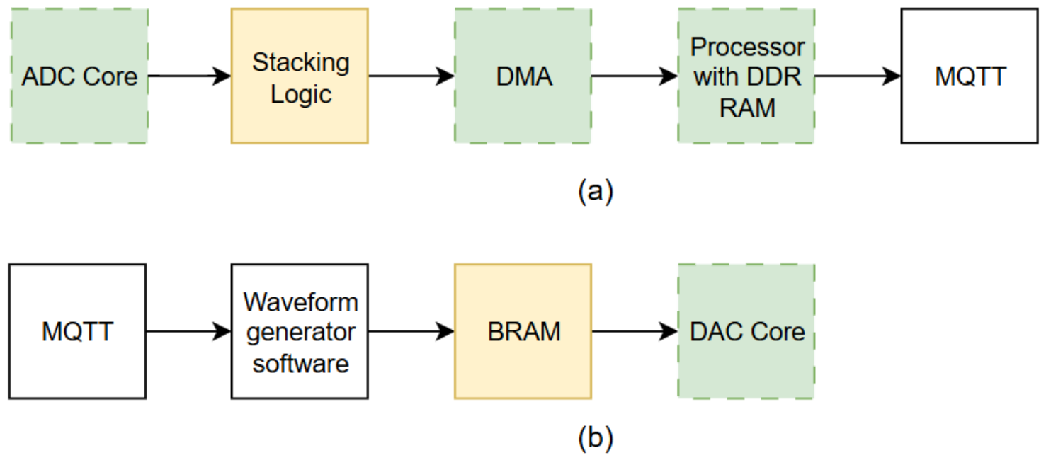
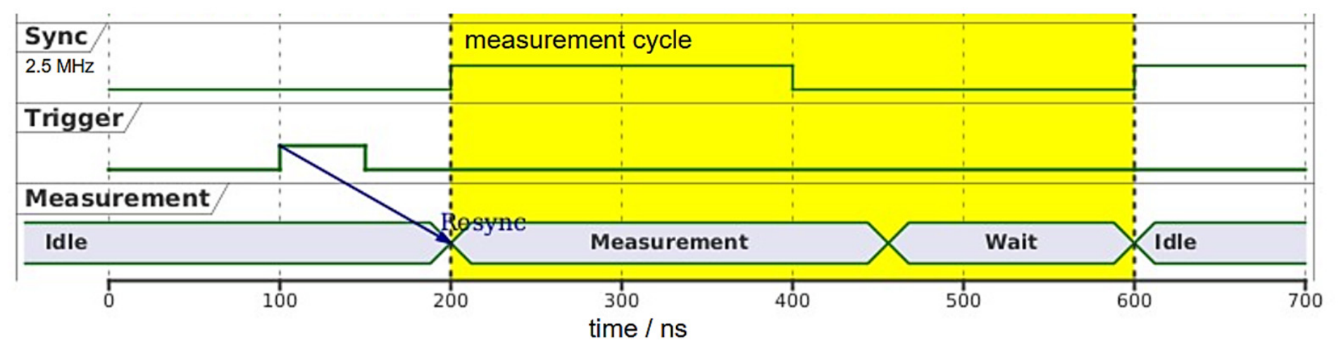
Data acquisition is performed with custom timing, illustrated in Figure 1. Frequency of the synchronization clock signal is 2.5 MHz, and the time allocated for measuring each frame is one clock cycle, 400 ns. During this cycle, the ADC digitizes 1024 samples over a 256 ns period. Afterwards, the system is idle for 144 ns. As illustrated in Figure 2a, after the ADC core acquires the frames, the stacking logic accumulates them in hardware.

To mitigate coherent system noise, a pulse inversion is also included in the stacking logic. The system is programmed to alternate the polarity of the transmitted pulse (0° and 180° phase shifts) for every consecutive frame. Received signals are inverted back to the original polarity before accumulation, so that the desired scattered signal gets constructively added and any constant background noise or coupling effects get canceled out.

The stacked data is then transferred via Direct Memory Access (DMA) to the processor’s DDR RAM, where it undergoes pre-processing before being sent over the network using the MQTT protocol.

MQTT is also used to configure the modules via the network. In particular, the waveform generator software is controlled via MQTT. Because the generation is realized by a DAC, an arbitrary waveform can be sent, and the software synthesizes the requested digital waveform and loads it into the FPGA’s on-chip Block RAM (BRAM) (see Figure 2b). Upon receiving the hardware trigger, the DAC reads the waveform data from the BRAM and converts it into an analog signal.

2.2. Source Waveform Generation

Three types of source waveforms were evaluated: a time-domain impulse based on a Ricker wavelet, SFCW and chirp. All waveforms were generated at a sampling rate of 4 GS/s and with identical peak-to-peak amplitude ($A$).

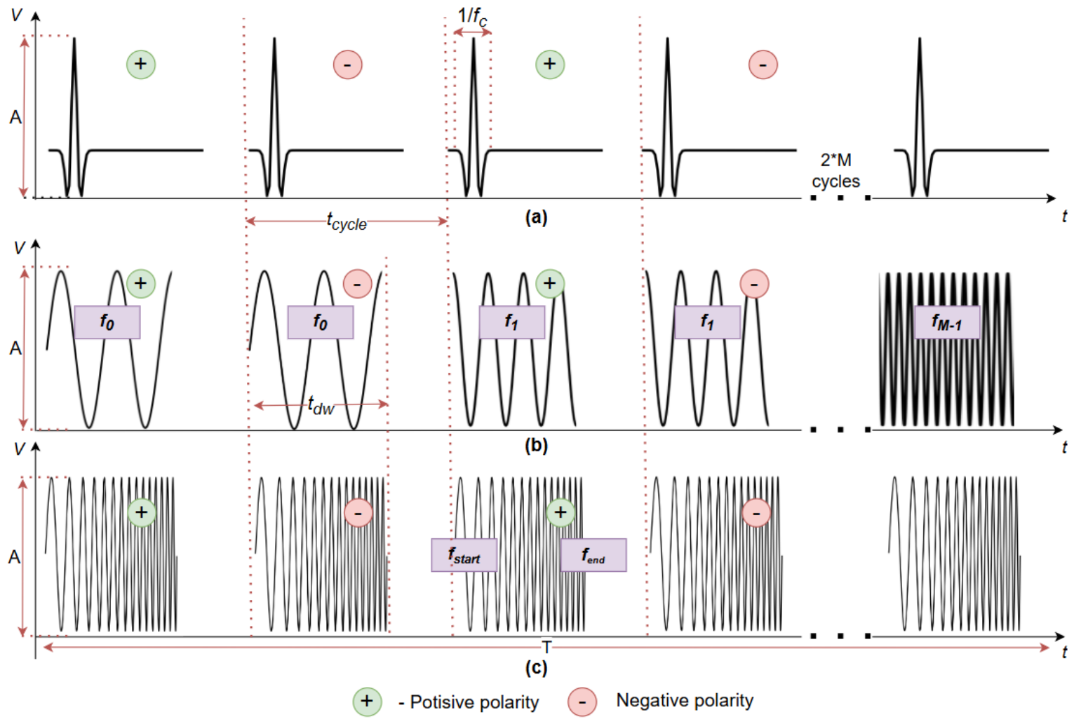
Figure 3 illustrates the temporal structure of the three waveforms. All waveforms were constrained to an identical total measurement time ($T$). The acquisition process is divided into discrete measurement cycles, denoted as $t_{cycle}$. Each cycle consists of an active transmission and reception window followed by hardware pause (256 and 144 ns regions from Figure 1). To reduce systematic noise, all waveforms are sent twice and with switched polarity, such that systematic errors are canceled in the stacking (averaging) process. For the SFCW method to successfully cancel coherent noise at every frequency step, each frequency must be transmitted for at least two cycles (one positive, one negative). To maintain an equivalent time budget, all three methods use a total of $2·M$ measurement cycles, where $M$ is the number of frequencies. The total measurement time is defined as

$$T=2·M·t_{cycle}$$

(1)

The simulations were executed with identical timing as measurements, although transmissions maintained constant polarity, since coherent noise was not modeled.

The impulse waveform (Figure 3a) was modeled as a Ricker wavelet, defined by its center frequency ($f_c$), which determines both the signal’s bandwidth and the width of the pulse in the time domain. A single impulse is transmitted per measurement cycle, and the alternating sequence is stacked over all $2·M$ cycles.

The SFCW waveform (Figure 3b) steps through a sequence of M discrete sinusoids from an initial frequency $f_0$ to a final frequency $f_{M-1}$. The system transmits each frequency for two consecutive cycles to perform the polarity alternation. The transmit duration within a measurement cycle is defined as dwell time ($t_{dw}$).

The chirp waveform (Figure 3c) sweeps from $f_{start}$ to $f_{end}$. The transmission time of the chirp was matched to $t_{dw}$. Like impulse, the chirp waveform is averaged across all cycles.

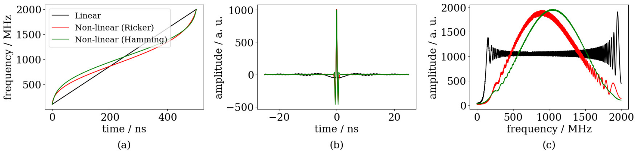
For the chirp waveform, a non-linear modulation technique was investigated. While a linear chirp sweeps frequencies at a constant rate, applying a non-linear modulation allows for the shaping of the signal’s spectrum (Figure 4c) by varying the sweep rate [26]. The chirp is designed to spend proportionally more time on frequencies where the amplitude is higher. This is achieved by defining the frequency-dependent timing function $t\left(f\right)$ based on the integral of the desired target spectrum, $W\left(f\right)$. The time $t$ at which a specific frequency f is reached is defined as

$$t\left(f\right)=t_{dw}{\displaystyle \frac{{\int }_{f_{start}}^{f}W\left(\nu \right)d\nu }{{\int }_{f_{start}}^{f_{end}}W\left(\nu \right)d\nu }}$$

(2)

By numerically inverting this relationship, the instantaneous frequency $f\left(t\right)$ as a function of time is calculated. The instantaneous phase $\varphi \left(t\right)$ is calculated by integrating $f\left(t\right)$ over time:

$$\varphi \left(t\right)=2\pi {\int }_0^{t}f\left(\tau \right)d\tau$$

(3)

The non-linear chirp transmit waveform $x\left(t\right)$ is then generated as a sinusoid:

$$x\left(t\right)=\mathrm{s}\mathrm{i}\mathrm{n}\left(\varphi \left(t\right)\right)$$

(4)

As demonstrated in Figure 4, the chirp waveform can be adapted to any spectral shape. However, this specific study uses Ricker wavelet distribution to match the source wavelet used in the impulse method.

The ripples in the reconstructed spectra (Figure 4c) are caused by discontinuities at the beginning and end of the chirp waveform. Truncating the frequency sweep is equivalent to multiplying the signal by a rectangular time window. This results in convolution of the spectrum with a sinc function [21], producing corresponding time-domain sidelobes. Strategies to mitigate these effects include weighting the spectrum or increasing the chirp duration to improve the time–bandwidth product.

The transmit waveforms for both simulations and measurements were generated using the following parameters: $f_c$ = 600 MHz; $M$ = 77; $f_{start}=f_0$ = 100 MHz; $f_{end}=f_M$ = 2000 MHz; and $t_{dw}$ = 120 ns.

These parameters were selected to balance the theoretical requirements of lysimeter tomography with the physical constraints of the hardware. The $f_c$ was selected as the common optimal value used for high-moisture soil monitoring. For the SFCW, frequency range and number of frequencies were tuned to include the relevant bandwidth of the antennas and prevent time-domain aliasing. $t_{dw}$ was limited to 120 ns by the buffer size in the current hardware configuration.

The total transmitted signal energy ($E_s$) for any given waveform $x\left(t\right)$ over the total measurement time $T$ is mathematically defined by the integral of its squared amplitude:

$$E_s={\int }_0^T{\left|x\left(t\right)\right|}^{2}dt$$

(5)

Because the hardware limits the maximum voltage to $A$, the energy allocation is dictated by the waveform’s duty cycle. The SFCW and chirp transmit for 120 ns per cycle. In contrast, the impulse is transmitted very briefly (approximately 3 ns for 600 MHz center frequency) and the transmitter is idle for the remainder of the cycle. Therefore, despite the identical time budgets, the SFCW and chirp methods send significantly more energy into the target medium.

Assuming an identical amplitude of $A$ = 1.4 V, the total signal energies ($E_s$) for the three waveforms were numerically evaluated using a discrete representation of the energy integral, yielding $7.7·{10}^{-8}$ V²∙s for impulse, $4.5·{10}^{-6}$ V²∙s for chirp and $4.4·{10}^{-6}$ V²∙s for SFCW.

2.3. Post-Processing

The digital post-processing requirements vary significantly depending on the chosen transmit waveform. To ensure a valid comparison for time-domain analysis, all raw data was processed to yield a real-valued, time-domain output, $Y\left[n\right]$.

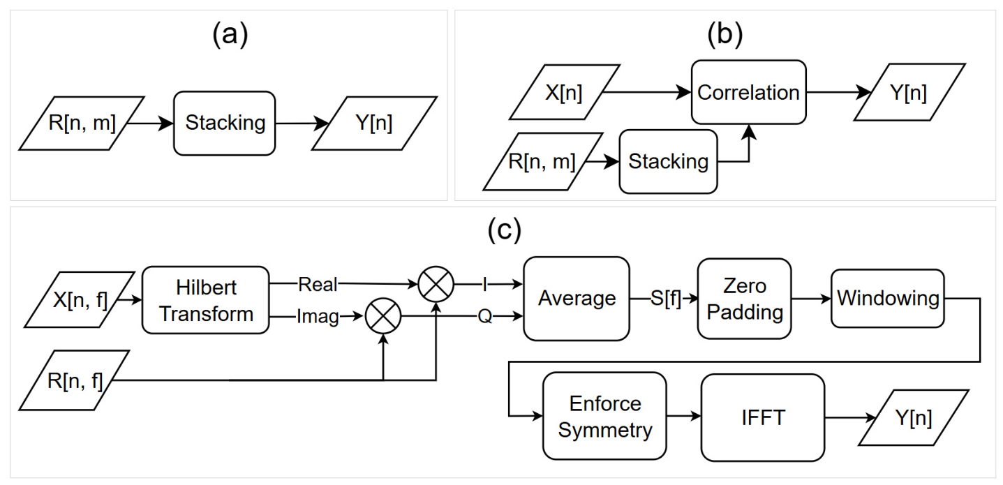
Because the impulse GPR inherently acquires data in the time domain, its processing chain is rather simple. The post-processing step is stacking (Figure 5a), which involves inverting the negative polarity traces and averaging multiple sequential traces represented as a two-dimensional array, $R[n, m]$, where n is the discrete time index and m represents the stack index. Assuming the presence of uncorrelated Gaussian white noise, this stacking process improves the SNR by a factor proportional to the number of stacked frames.

In the processing chain for the chirp method (Figure 5b), the received signal is first stacked in the same manner as the impulse method. The frequency sweep of the chirp is modulated with a non-linear function that mimics a Ricker wavelet (Figure 4), suppressing sidelobes directly during the correlation stage.

The processing of SFCW data is more complicated, as it requires converting a sequence of measurements at different frequencies into a synthetic time-domain signal. The digital signal processing chain implemented for this conversion is illustrated in Figure 5c.

For each frequency step, the two phase-alternated measurement cycles are subtracted to form a single noise-canceled trace, $R[n, f]$ (where $f$ is the frequency index), and quadrature demodulation is performed to extract the in-phase ($I$) and quadrature ($Q$) components. This is achieved in the digital domain by multiplying $R[n, f]$ with reference signals derived from the transmitted waveform $X[n, f]$. The references are generated via a Hilbert transform of $X[n, f]$. The resulting $I$ and $Q$ signals are then averaged and a single complex value, $S\left[f\right]=I\left[f\right]+jQ\left[f\right]$, is produced. This value represents the magnitude and phase of the systems’ response at a specific frequency.

This process is repeated for every frequency step until the full spectrum is assembled. Before transforming to the time domain, several steps are applied: Zero-padding is performed to correctly place the measured frequency components into their corresponding discrete frequency bins (from DC to Nyquist frequency). To mitigate time-domain sidelobes, the SFCW spectrum is weighted by a window with the shape of the spectrum of a Ricker wavelet. The center frequency of this window matches the center frequency of the impulse GPR waveform under comparison. Applying this window ensures a consistent pulse shape across methods, enabling direct comparison between the reconstructed time-domain signals and results obtained from the impulse method. To ensure that the final output is a real-valued signal, Hermitian symmetry is enforced on the spectrum. Finally, an inverse fast Fourier transform generates the synthetic time-domain signal, $Y\left[n\right]$. Note that the windowing causes a portion of the energy in the received signal to be discarded.

2.4. Numerical Simulation Framework and Electromagnetic Modeling

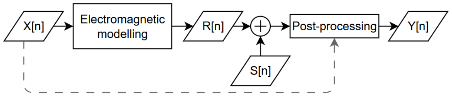
To investigate the performance of the impulse, SFCW and chirp waveforms under idealized conditions, a numerical simulation workflow, illustrated in Figure 6, was established. The entire framework, except for electromagnetic modeling, was implemented using the Python (version 3.12.3) programming language.

The simulation begins with the digital generation of a source waveform, $X\left[n\right]$. This signal is then passed through a transfer function obtained from electromagnetic modeling in CST Studio Suite 2025 by Dassault Systèmes Simulia (Vélizy-Villacoublay, France). The resulting received signal, $R\left[n\right]$, is contaminated with synthetic Gaussian noise, $S\left[n\right]$. The same noise realization was used for all three methods to ensure a fair comparison. In the physical environment, the system is subjected to different noise sources, which cannot be generalized. By utilizing white Gaussian noise, the simulation-based study establishes an upper bound for waveform performance in terms of the signal-to-noise ratio.

The noisy signal undergoes post-processing steps (Figure 5) to produce a single time-domain trace, $Y\left[n\right]$. As indicated by the dashed line in Figure 6, this stage also incorporates the $X\left[n\right]$ in the case of SFCW and chirp processing.

To obtain the system’s transfer function, a 3D electromagnetic model was developed using CST Studio Suite. The simulation consists of two antennas facing each other with a separation of 1 m. This replicates the experimental setup. The distance of 1 m was chosen based on the diameter of the lysimeter.

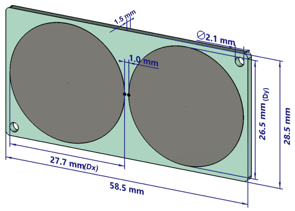
The antenna utilized in the simulation is the custom planar elliptical PCB dipole designed for the SMUCT-GPR system. The physical dimensions of the antenna PCB are detailed in Figure 7. Further details regarding the antenna design and modeling can be found in [27].

The simulation was executed using the CST time domain solver, utilizing a hexahedral mesh. The frequency range was defined to be from 0.1 GHz to 2.0 GHz.

Upon completion, the simulation results were exported as a Touchstone file (.s2p). The forward transmission coefficient ($S_{21}$) was extracted to represent the transfer function, where Antenna 1 acts as a transmitter and Antenna 2 acts as the receiver. Using a custom Python script, this frequency-domain data was converted into the system’s time-domain impulse response via inverse Fourier transform. Finally, to simulate the raw signals, ($R\left[n\right]$), captured by the ADCs, this impulse response was convolved with the source waveforms.

2.5. Measurement Setup

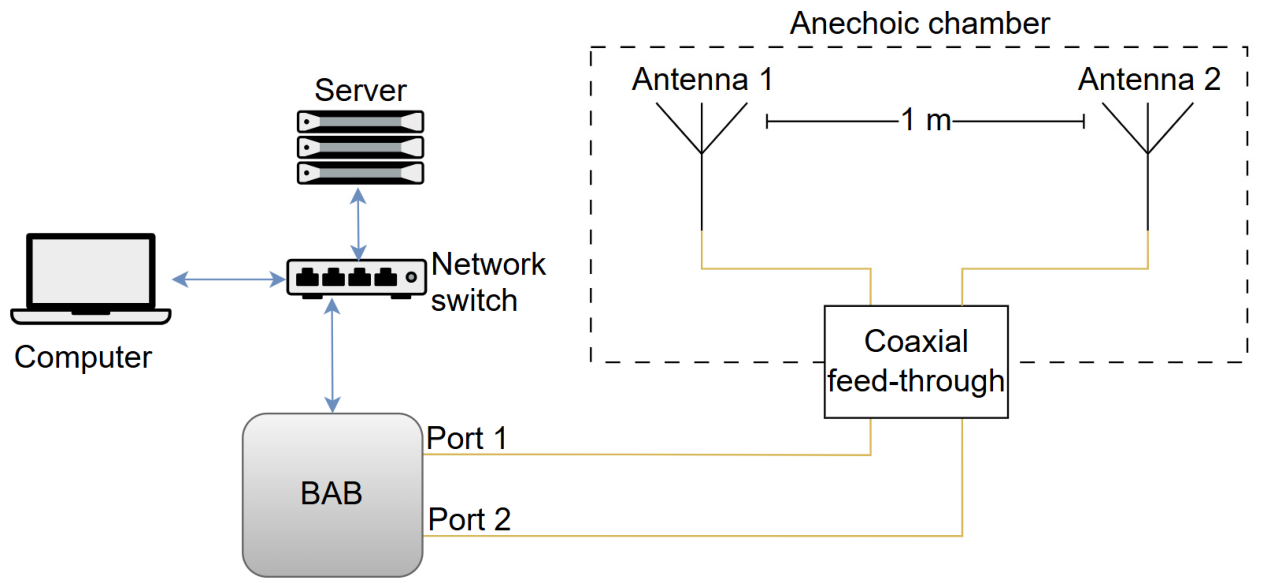
To minimize reflections from the environment and radio frequency interference, the experiments with the antennas were performed inside an anechoic chamber. Two ports of the 64-port BAB were connected to the transmitting and receiving antennas via coaxial cables. These cables were routed into the isolated environment using a coaxial feed-through panel of the chamber wall. Figure 8 represents the block diagram of this setup, where “Antenna 1” and “Antenna 2” are two planar elliptical dipoles.

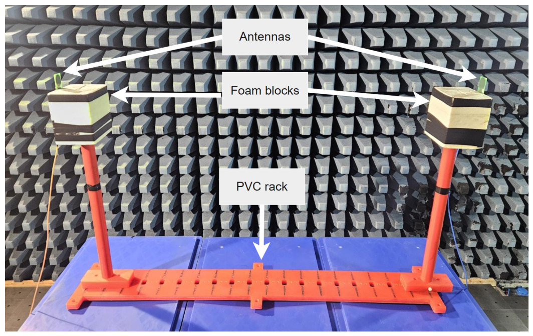
Inside the chamber, the antennas were positioned to face each other at a separation distance of 1 m. A custom mechanical mount was constructed from polyvinyl chloride (PVC). The antennas and the ends of the coaxial cables were secured with a tape to the blocks of foam, which have a low dielectric constant (Figure 9).

The measurement procedure was performed with the help of a dedicated computer connected to the BAB via a local network switch. A custom Python script was developed to manage bidirectional communication with the BAB. This script utilized the MQTT protocol to transmit the instructions over the network, commanding the BAB to generate the source waveforms, digitize the incoming signals at the receiver, perform hardware-level stacking and transmit the resulting signals back to the computer. The acquired measurement data were saved in .npy format for post-processing and visualization.

3. Results

3.1. Simulation

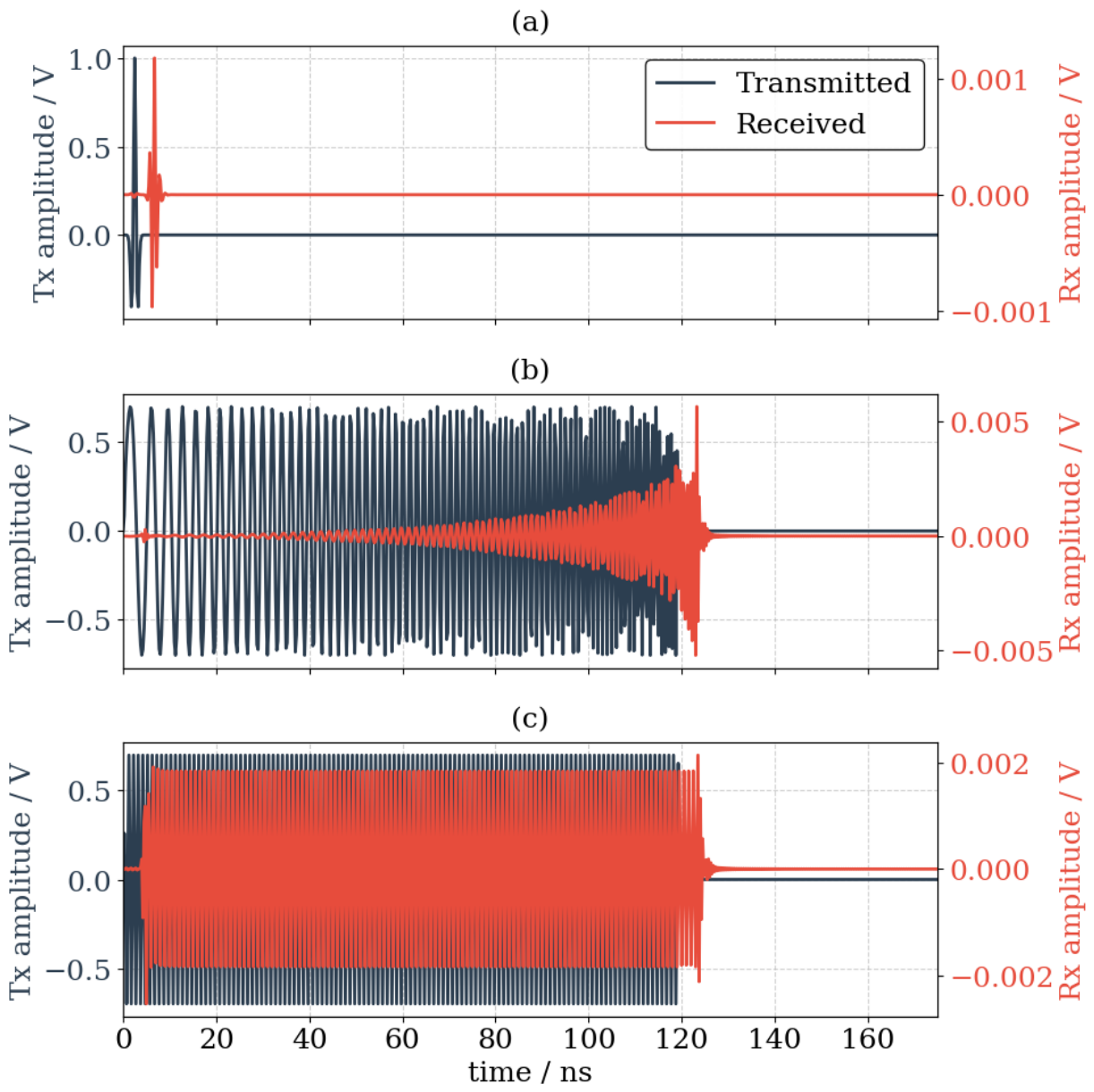
The generated source waveforms and their corresponding received signals—obtained after convolving the inputs with the system’s transfer function—are presented in Figure 10.

White Gaussian noise with a mean of zero and standard deviation of 0.005 V was added to all three received waveforms. The noiseless signals were stored separately as a reference.

SNR was calculated as the ratio of the total signal energy to the total noise energy. For the post-processed signals (following the processing stages illustrated in Figure 5), the noise was isolated by subtracting the ideal processed output (derived from the noiseless input signals) from the noisy processed output. This noise-addition and evaluation sequence was executed over 100 independent iterations. The final SNR values reported in this study represent the average across all trials to ensure consistent results.

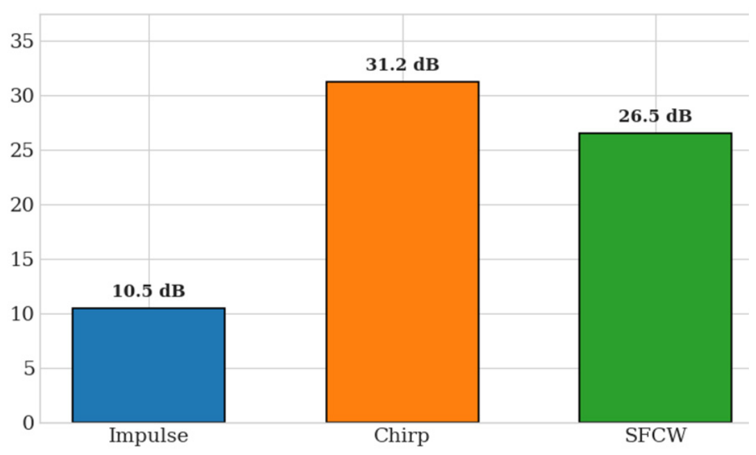
Figure 11 illustrates the final SNR of the post-processed signals. The impulse waveform has the lowest SNR. Although utilizing the same voltage range, the impulse signal has a low duty cycle. It is only actively transmitted for a fraction of the time window. Therefore, the total transmitted signal energy is lower than that of the chirp and SFCW.

Both the chirp and SFCW methods outperform the impulse method with final SNRs of 31.2 and 26.5 dB (Figure 11). The non-linear chirp has the highest performance, because its spectral shaping prevents the need for digital windowing applied to the SFCW spectrum, which reduces the useful signal energy.

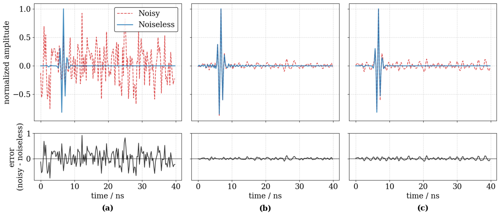
While the SNR results from Figure 11 quantify the suppression of random thermal noise, a close examination of the processed time-domain signals provides a visual representation of this noise mitigation. Figure 12 overlays the final processed time-domain signals derived from both noisy and noiseless inputs for all three methods. To isolate and visualize the effect of added noise, the error plot beneath each waveform displays the difference between the noisy and noiseless processed signals.

The error plots visually confirm the advantage in SNR of sinewave-based methods. The impulse method (Figure 12a) exhibits a higher amplitude compared to the other two methods.

Reconstructed noiseless chirp (blue trace on Figure 12b) reveals deterministic artifacts in the output. They are visible as small amplitude fluctuations preceding and following the main pulse between 5 and 10 ns. These deviations are caused by discontinuities in the beginning and end of the transmitted waveform, which produce spectral “ripples” visible in the frequency domain (Figure 4). In physical applications, these artifacts could mask the detection of weak scatterings. Strategies to mitigate these effects include extending the temporal length of the chirp or applying digital amplitude tapering to the waveform.

3.2. Experiment

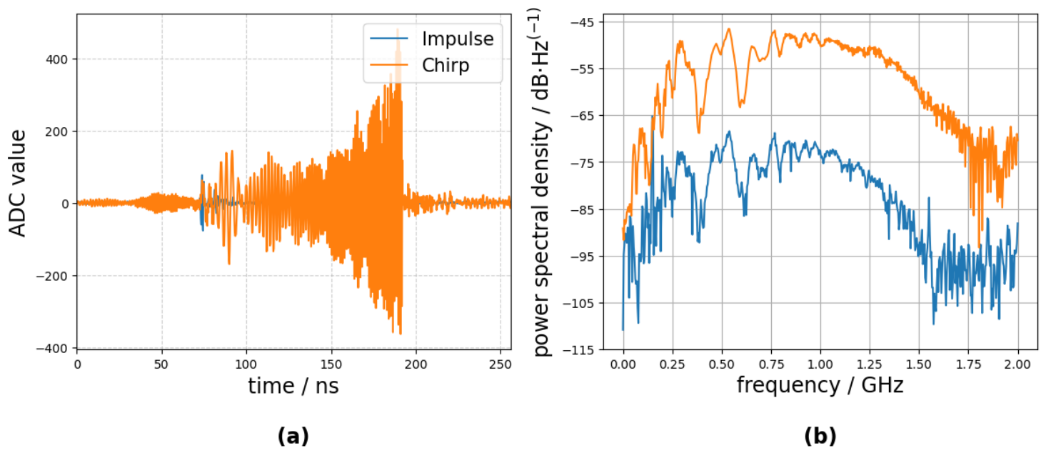
The experimental measurements utilized waveform parameters identical to those defined in the numerical simulations. Figure 13 displays the received signals for the impulse and non-linear chirp methods following the 154 polarity-alternating stacks (corresponding to the $2·M$ measurement cycles defined in Section 2.2). The time-domain inspection of these signals (Figure 13a) reveals some signal activity preceding the primary wave arrival (between 50 and 100 ns). This is attributed to internal on-board electromagnetic coupling on the BAB.

The energy difference between the impulse and the 120 ns chirp is evident in both the time and frequency domains. For the impulse, the high-frequency components above approximately 1.25 GHz (Figure 13b) degrade into the noise floor. In contrast, the chirp waveform maintains signal integrity up to 1.75 GHz.

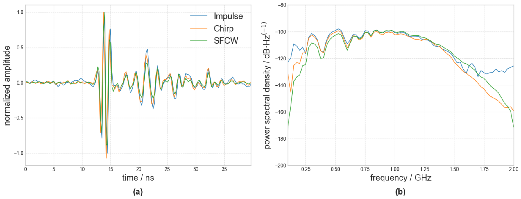
Following the application of the digital signal processing pipelines, the chirp and SFCW waveforms were converted into synthetic time-domain pulses. Figure 14 presents the final outputs for all three methods, alongside their power spectral densities. To compare the shapes, the time-domain signals have been normalized, cropped and overlaid. The frequency-domain conversion was applied to the normalized signals.

In the time domain (Figure 14a), both the chirp and SFCW have reconstructed the shape of the pulse. Secondary oscillations are visible immediately following the main pulse (after 15 ns) across all three methods. These late arrivals come from the reflections of the testing environment. The absorbing material lining the anechoic chamber is less effective at attenuating the lower-frequency components.

There is noticeable variance, especially near the peak amplitudes, among the normalized traces.

Evaluating these processed signals in the frequency domain (Figure 14b) reveals visible differences in the noise floor above 1.5 GHz. Both the SFCW and chirp methods offer cleaner representation in this frequency range compared to the impulse.

To quantify the SNR, noise measurements were conducted. For each method, null transmissions (zero-amplitude signals) were sampled with the ADC. These signals were processed through the exact same digital pipelines (Figure 5) used for the active signals. Defining the energy of this processed noise output as $E_N$, and the energy of the actively measured, post-processed signal as $E_{S+N}$, the SNR was estimated using the following ratio:

$$SNR={\displaystyle \frac{E_{S+N}-E_N}{E_N}}$$

(6)

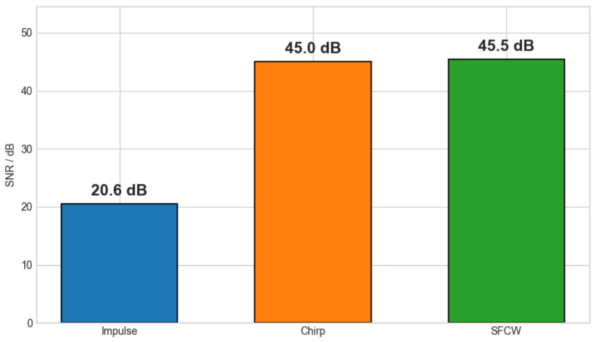
The results of this calculation are presented in Figure 15. To sum up the results, SNR values for simulations were 10.5 dB for the impulse, 31.2 dB for the chirp and 26.5 dB for SFCW. The measurements resulted in 20.6 dB for the impulse, 45.0 dB for the chirp and 45.5 dB for the SFCW. In both investigations, the chirp methods improve the SNR by over 20 dB compared to the impulse.

4. Discussion

Both numerical simulations and physical experiments demonstrated that the sinewave-based methods yield better SNR compared to the impulse approach. Under idealized simulation conditions, the non-linear chirp demonstrated the best SNR. In the measurements, SFCW and chirp also showed improvement over the impulse. Because the noise level in the simulations was defined arbitrarily, a direct comparison of SNR values between the simulated and measured cases is uninformative. Instead, relative performance differences are examined. In the simulations, the chirp and SFCW methods outperformed the impulse method by 20.7 dB and 16.0 dB, respectively. The results were different in the experiment, which showed 24.4 dB improvement for the chirp and 24.9 dB for the SFCW. The reason for this difference between simulation and measurement needs to be further investigated. Comparing chirp and SFCW methods, simulations predicted a 4.7 dB advantage for chirp, while the experimental results showed that SFCW performed better by 0.5 dB. To quantify the SNR difference precisely, testing must incorporate averaging over many measurements to estimate mean SNR.

SFCW-based implementations require the most complex processing pipeline. In contrast, non-linear chirp achieves comparable noise suppression but simplifies the signal processing implementation. However, the chirp method leads to time-domain sidelobes, which can be reduced through additional processing or adjusting of the waveform parameters.

A strict requirement for the targeted lysimeter tomography application is the ability to feed time-domain data into an FWI algorithm. Through the simulations and measurements, it was demonstrated that with appropriate processing, both sinusoidal waveform-based methods can reconstruct the required pulse shape.

5. Conclusions

While the advantages of the SFCW and frequency-modulated radars over the impulse systems are well-documented in the literature, comparative studies in the cases of GPR systems often suffer from hardware bias. Evaluations comparing commercial impulse and continuous-wave GPR systems have relied on different antenna designs and analog front-ends, making it difficult to isolate the performance of the waveform itself.

The primary contribution of this study is the evaluation of impulse, SFCW and chirp waveforms utilizing an identical software-defined radio (SDR) architecture based on a high-speed RFSoM and elliptical dipole antennas. By constraining the comparison to a unified time budget and identical amplitudes, this study provides an objective evaluation of the waveform performance.

Both numerical simulations and physical experiments quantified the SNR advantage of the chirp and SFCW methods over the impulse approach under the given parameter selection by more than 20 dB and 16 dB, respectively. The advantage was even larger for the simulations, which needs to be further investigated.

Compared to the impulse method, the chirp method presents an advantage in firmware implementation. The pulse compression for the chirp requires only a single cross-correlation step. Due to this ease of real-time implementation, the non-linear chirp waveform will be considered for the final SMUCT-GPR system.

The transition from simulation to physical experimentation highlighted the practical constraints of SDR development. Specifically, the existing firmware implementation and the DAC buffer size prevented continuous transmission of the long chirp waveforms. The next step in this research is to implement continuous chirp transmission and real-time matched-filtering logic directly in the firmware, eliminating the need for signal stacking.

In addition, the frequency content of the non-linear chirp could be tailored to the environment. The electromagnetic characteristics of the medium in between the antennas influence the transfer function of the system. For example, the presence of high-moisture mediums, such as pure water, vapor or wet soil, in between the antennas attenuates energy in the region somewhere above 1 GHz. In such environments, a non-linear chirp’s modulation profile can be adjusted to concentrate transmission energy to maximize penetration depth and measurement accuracy.

References

1. Jol, H.M. Ground Penetrating Radar Theory and Applications; Elsevier: Amsterdam, The Netherlands, 2008; ISBN 978-0-08-095184-3. [Google Scholar]
2. Abdulraheem, M.I.; Chen, H.; Li, L.; Moshood, A.Y.; Zhang, W.; Xiong, Y.; Zhang, Y.; Taiwo, L.B.; Farooque, A.A.; Hu, J. Recent Advances in Dielectric Properties-Based Soil Water Content Measurements. Remote Sens. 2024, 16, 1328. [Google Scholar] [CrossRef]
3. Lombardi, F.; Ortuani, B.; Facchi, A.; Lualdi, M. Assessing the Perspectives of Ground Penetrating Radar for Precision Farming. Remote Sens. 2022, 14, 6066. [Google Scholar] [CrossRef]
4. Gonzales, E.; Ticona, J.; Minaya, A.; Krahenbuhl, R.; Shragge, J.; Low, J.; Flamme, H. Geophysical Mapping of Cemented Subsoils for Agricultural Development in Southern Peru. Sustainability 2024, 16, 6801. [Google Scholar] [CrossRef]
5. Klotzsche, A.; Vereecken, H.; van der Kruk, J. Review of Crosshole Ground-Penetrating Radar Full-Waveform Inversion of Experimental Data: Recent Developments, Challenges, and Pitfalls. Geophysics 2019, 84, H13–H28. [Google Scholar] [CrossRef]
6. Bräunlich, N.; Wagner, C.W.; Sachs, J.; Del Galdo, G. Configurable Pseudo Noise Radar Imaging System Enabling Synchronous MIMO Channel Extension. Sensors 2023, 23, 2454. [Google Scholar] [CrossRef] [PubMed]
7. Lukin, K.; Vyplavin, P.; Palamarchuk, V.; Lukin, S.; Mischenko, E.; Zaets, N. Radar Tomography Using MIMO Noise Radar with Signals Time-Division in Transmit/Receive Channels. In Proceedings of the 2015 IEEE Radar Conference (RadarCon), Arlington, VA, USA, 10–15 May 2015; pp. 1461–1463. [Google Scholar]
8. Rial, F.I.; Lorenzo, H.; Pereira, M.; Armesto, J. Waveform Analysis of UWB GPR Antennas. Sensors 2009, 9, 1454–1470. [Google Scholar] [CrossRef] [PubMed]
9. Schettino, A.; Ghezzi, A.; Tassi, L.; Catapano, I.; Persico, R. Trace Modelling: A Quantitative Approach to the Interpretation of Ground-Penetrating Radar Profiles. Remote Sens. 2026, 18, 208. [Google Scholar] [CrossRef]
10. Wang, Y. The Ricker Wavelet and the Lambert W Function. Geophys. J. Int. 2015, 200, 111–115. [Google Scholar] [CrossRef]
11. Wang, Y. Frequencies of the Ricker Wavelet. Geophysics 2015, 80, A31–A37. [Google Scholar] [CrossRef]
12. Tronca, G.; Tsalicoalou, I.; Lehner, S.; Catanzariti, G. Comparison of Pulsed and Stepped Frequency Continuous Wave (SFCW) GPR Systems. In Proceedings of the 2018 17th International Conference on Ground Penetrating Radar (GPR), Rapperswil, Switzerland, 18–21 June 2018; pp. 1–4. [Google Scholar] [CrossRef]
13. Eide, E.; Linford, N.; Persico, R.; Sala, J. Chapter 8—Advanced SFCW GPR Systems. In Innovation in Near-Surface Geophysics; Persico, R., Piro, S., Linford, N., Eds.; Elsevier: Amsterdam, The Netherlands, 2019; pp. 253–285. ISBN 978-0-12-812429-1. [Google Scholar]
14. Lambot, S.; Slob, E.C.; van den Bosch, I.; Stockbroeckx, B.; Scheers, B.; Vanclooster, M. Estimating Soil Electric Properties from Monostatic Ground-Penetrating Radar Signal Inversion in the Frequency Domain. Water Resour. Res. 2004, 40, W04205. [Google Scholar] [CrossRef]
15. Lombardi, F.; Lualdi, M. Step-Frequency Ground Penetrating Radar for Agricultural Soil Morphology Characterisation. Remote Sens. 2019, 11, 1075. [Google Scholar] [CrossRef]
16. Persico, R.; Ciminale, M.; Matera, L. A New Reconfigurable Stepped Frequency GPR System, Possibilities and Issues; Applications to Two Different Cultural Heritage Resources. Near Surf. Geophys. 2014, 12, 793–801. [Google Scholar] [CrossRef]
17. Seyfried, D.; Busche, A.; Janning, R.; Schmidt-Thieme, L.; Schoebel, J. Information Extraction from Ultrawideband Ground Penetrating Radar Data: A Machine Learning Approach. In Proceedings of the 2012 The 7th German Microwave Conference, Ilmenau, Germany, 12–14 March 2012; pp. 1–4. [Google Scholar]
18. Seyfried, D.; Schoebel, J. Stepped-Frequency Radar Signal Processing. J. Appl. Geophys. 2015, 112, 42–51. [Google Scholar] [CrossRef]
19. Stove, A.G. Linear FMCW Radar Techniques. IEE Proc. F (Radar Signal Process.) 1992, 139, 343–350. [Google Scholar] [CrossRef]
20. Paun, M. Through-Wall Imaging Using Low-Cost Frequency-Modulated Continuous Wave Radar Sensors. Remote Sens. 2024, 16, 1426. [Google Scholar] [CrossRef]
21. Klauder, J.R.; Price, A.C.; Darlington, S.; Albersheim, W.J. The Theory and Design of Chirp Radars. Bell Syst. Tech. J. 1960, 39, 745–808. [Google Scholar] [CrossRef]
22. Tilley, R.; Sadjadpour, H.R.; Dowla, F. GPR Imaging for Deeply Buried Objects: A Comparative Study Based on Compositing of Scanning Frequencies and a Chirp Excitation Function. Geosciences 2019, 9, 132. [Google Scholar] [CrossRef]
23. Mester, A.; Bachner, M.; Schardt, G.; Chkhetia, R.; Silex, W.; Krenz, E.; Rongen, H.; Zimmermann, E.; Klotzsche, A.; Natour, G. Design of a Novel Scalable Multi-Channel GPR System for High-Resolution High-Speed Tomography of Soil Columns. In Proceedings of the European Geosciences Union General Assembly 2025 (EGU25), Vienna, Austria, 27 April–2 May 2025. [Google Scholar] [CrossRef]
24. Neumann, J.; Brüggemann, N.; Chaumet, P.; Hermes, N.; Huwer, J.; Kirchner, P.; Lesmeister, W.; Mertens, W.A.; Pütz, T.; Wolters, J.; et al. The AgraSim (Agricultural Simulator) Facility for the Comprehensive Experimental Simulation and Analysis of Environmental Impacts on Processes in the Soil-Plant-Atmosphere System. EGUsphere 2024, 2024, 1–28. [Google Scholar] [CrossRef]
25. Bekman, I.; Mester, A.; Roth, C.; Zimmermann, E.; Schardt, G.; Rongen, H.; Heggen, J.; Wüstner, P.; Heil, R.; van Waasen, S. Clock Synchronization for a Multidevice Data Acquisition System of a Ground Penetrating Radar; Zentralinstitut für Elektronik: Jülich, Germany, 2023. [Google Scholar] [CrossRef]
26. Doerry, A. Generating Nonlinear FM Chirp Waveforms for Radar; Sandia National Laboratories: Livermore, CA, USA, 2006; p. SAND2006-5856. [Google Scholar]
27. Chkhetia, R.; Schreckenberg, L.; Mester, A.; Zimmermann, E.; Natour, G. Optimization of a 900 MHz Elliptical Dipole Antenna for a GPR Monitoring System. 2026. Available online: https://juser.fz-juelich.de/record/1056169 (accessed on 1 June 2026).
Figure 1. Timing diagram for the measurement sequence as it is implemented in the current firmware of our baseboard. One complete measurement cycle is highlighted in yellow.
Applsci 16 06179 g001
Figure 2. High-level block diagrams for the (a) data acquisition and (b) waveform generation processes.
Applsci 16 06179 g002
Figure 3. Sketch of (a) impulse, (b) SFCW and (c) chirp waveforms along with their transmission parameters. (“*” in “2*M cycles” represents multiplication).
Applsci 16 06179 g003
Figure 4. Linear chirp and two non-linear chirps with different spectral distributions and their influence on autocorrelation result. (a) Time vs. frequency sweep profiles. (b) Resulting autocorrelation functions in time domain. (c) Corresponding autocorrelation spectra in the frequency domain.
Applsci 16 06179 g004
Figure 5. Signal processing chains for (a) impulse, (b) chirp and (c) SFCW methods.
Applsci 16 06179 g005
Figure 6. Block diagram of the complete simulation workflow. The electromagnetic modeling refers to a three-dimensional realization of the antenna setup in CST Studio. The dashed line indicates that the reference signal X [ n ] is utilized in the post-processing for the SFCW and chirp, but not for impulse method.
Applsci 16 06179 g006
Figure 7. Antenna modeling details: model of a single planar elliptical dipole PCB with dimensions in mm.
Applsci 16 06179 g007
Figure 8. High-level block diagram of the measurement setup.
Applsci 16 06179 g008
Figure 9. Measurement setup in the anechoic chamber: antenna mount on the PVC rack with a separation of one meter.
Applsci 16 06179 g009
Figure 10. A temporal section of the generated input waveforms (black) and the resulting output signals (red) obtained via convolution with the system’s transfer function for three methods: (a) impulse, (b) chirp and (c) SFCW (only 1000 MHz sinewave).
Applsci 16 06179 g010
Figure 11. Calculated SNR for the three evaluated methods after post-processing (average over 100 iterations).
Applsci 16 06179 g011
Figure 12. Processed time-domain outputs with normalized amplitudes, comparing the signals from noisy and noiseless inputs for the (a) impulse, (b) chirp and (c) SFCW methods. The residual error is plotted beneath each figure.
Applsci 16 06179 g012
Figure 13. Received signals for the impulse and non-linear chirp transmit waveforms in the (a) time domain and (b) frequency domain (power spectral density).
Applsci 16 06179 g013
Figure 14. Reconstructed outputs of the impulse, chirp and SFCW methods. (a) Normalized time-domain signals. (b) Frequency-domain power spectral densities.
Applsci 16 06179 g014
Figure 15. SNR of the measured signals after post-processing for the three methods.
Applsci 16 06179 g015
Disclaimer/Publisher’s Note: The statements, opinions and data contained in all publications are solely those of the individual author(s) and contributor(s) and not of MDPI and/or the editor(s). MDPI and/or the editor(s) disclaim responsibility for any injury to people or property resulting from any ideas, methods, instructions or products referred to in the content.