Estimating Light-Duty Vehicle Fuel Consumption and CO₂ Emissions via OBD-II Speed-Density Modeling: A Field Demonstration

Abstract

Laboratory-based certification cycles systematically underestimate real-world fuel consumption and CO₂ emissions. On-board diagnostics (OBD-II) telemetry offers a low-cost alternative, yet most published approaches rely on mass air flow (MAF) sensors absent from many modern vehicles. This study validates a speed-density air-mass estimation method on a naturally aspirated RON 95 gasoline passenger car (1368 cm³, Euro 6) across seven drive cycles recorded over three measurement days in northwestern Türkiye, covering 609.6 km of highway, urban, and mixed conditions. Instantaneous air mass flow was estimated from four standard OBD-II PIDs—manifold absolute pressure, engine speed, intake air temperature, and fuel trim corrections—using the ideal gas law applied to actual engine displacement. Results were validated against pump-measured fill-up volumes. The speed-density model achieved errors of −3.6% to +4.3% across individual segments (combined error: −0.5%), outperforming the vehicle’s onboard trip computer, which exhibited errors of −10.6% to +14.6%. Derived CO₂ intensities ranged from 125.0 to 166.4 g/km, with a combined average of 147.2 g/km (pump reference: 147.9 g/km). Urban driving produced approximately 15% higher specific emissions than highway driving. These results demonstrate that a physics-based speed-density model can achieve within ±5% trip-level accuracy across diverse real-world conditions without machine learning, bespoke calibration, or a physical MAF sensor.

1. Introduction

The gap between type-approval fuel economy figures and real-world consumption has been extensively documented. Koszałka et al. [1] reported that fuel consumption measured under the New European Driving Cycle (NEDC) could be up to 50% lower than real-world figures, a discrepancy that persisted even after the introduction of the Worldwide Harmonized Light Vehicle Test Procedure (WLTP) in 2017. Pavlovic et al. [2] confirmed that real-world CO₂ improvements have consistently lagged behind type-approval progress over the preceding decade. This divergence motivates the development of portable, vehicle-agnostic methods for measuring fuel consumption and carbon footprint under actual driving conditions.

OBD-II diagnostic interfaces, mandatory on all petrol vehicles sold in the European Union since 2001, provide real-time access to a standardized set of engine parameters at polling rates of 1–240 Hz [3,4,5,6]. Several studies have exploited this accessibility for fuel consumption estimation. Malekian et al. [7] demonstrated an OBD-II fleet management system capable of computing fuel consumption from vehicle speed and mass air flow. Abukhalil et al. [8] employed a support vector machine trained on OBD-II features to estimate fuel consumption across multiple vehicles and routes. Abediasl et al. [3] developed real-time instantaneous fuel estimation using machine learning on OBD-II data collected from fleet vehicles. A common dependency across these approaches is the Mass Air Flow (MAF) sensor signal (OBD PID 0x0110), which provides a direct measurement of inducted air mass and, combined with the stoichiometric air–fuel ratio, yields fuel flow. However, a substantial fraction of modern passenger cars—particularly smaller-displacement naturally aspirated engines—rely on speed-density strategies in the engine control unit (ECU) rather than a physical MAF sensor. For these vehicles, PID 0x0110 is either unavailable or returns a software-derived estimate of uncertain provenance, limiting the applicability of MAF-centric estimation methods.

Speed-density estimation reconstructs air mass flow from the ideal gas law applied to the intake manifold, using Manifold Absolute Pressure (MAP), Revolutions per Minute (RPM), Intake Air Temperature (IAT), and a volumetric efficiency (VE) parameter. This approach is well established in ECU design [9] and has been applied to engine modeling and torque estimation, but pump-validated fuel consumption results from field experiments remain sparse in the open literature.

The present study addresses this gap with a controlled field experiment using a single naturally aspirated gasoline vehicle on seven distinct drive cycles across northwestern Türkiye. The specific contributions are: (1) a pump-validated demonstration that the speed-density model achieves within ±5% fuel estimation error across highway and urban conditions; (2) a quantitative comparison showing consistently smaller errors than the vehicle’s onboard trip computer; (3) a drive-cycle-resolved CO₂ footprint characterization showing a ~15% urban penalty relative to highway driving; and (4) evidence that the method requires no machine learning, no training data, and no vehicle-specific calibration beyond publicly available engine displacement data.

2. Materials and Methods

2.1. Test Vehicle and Instrumentation

The test vehicle was a 2025 Fiat Egea Cross (Türk Otomobil Fabrikası A.Ş., Bursa, Türkiye) equipped with a 1.4 L naturally aspirated port fuel-injected (PFI) gasoline engine (displacement: 1368 cm³, rated power: 70 kW at 6000 rpm), compliant with Euro 6 emission standards and fueled exclusively with RON 95 unleaded petrol throughout all trials. The vehicle’s ECU employs a speed-density fueling strategy and does not carry a physical MAF sensor; OBD PID 0x0110 is therefore excluded from all analyses.

OBD-II data were acquired via a Wi-Fi ELM327 adapter (Shenzen Lonauto Technology Co., Ltd., Shenzen, China) connected to a custom Android application (

Table 1. OBD-II parameter identifiers (PIDs) polled by the data-acquisition application.

PID	Parameter	Unit
0x010B	Manifold Absolute Pressure (MAP)	kPa
0x010C	Engine Speed (RPM)	rev/min
0x010F	Intake Air Temperature (IAT)	°C
0x010D	Vehicle Speed	km/h
0x0106	Short-Term Fuel Trim (STFT, Bank 1)	%
0x0107	Long-Term Fuel Trim (LTFT, Bank 1)	%
0x012F	Fuel Level	%
0x0104	Calculated Engine Load	%

Concurrent GNSS position (latitude, longitude, altitude) was recorded via the smartphone’s internal receiver at the same 3 s cadence.

). The application polled the following PIDs at approximately 3 s intervals and logged each frame with a Unix millisecond timestamp:

2.2. Drive Cycles and Data Collection

Data were collected across three measurement days: 11 April, 29 May, and 30 May 2026. Seven drive cycles were defined by distinct fueling events (full pump fill-up at the start and end of each cycle), providing independent ground truth fuel volumes:

Drive Cycle 1 [DC1] (11 April-Highway Morning) was conducted on 11 April 2026 as an eastbound run along the D-100 state highway from Tekirdağ to Silivri, with departure at 09:26 local time. Total distance was 73.1 km as determined by OBD-II vehicle speed integration, and elapsed duration was 57.4 min, yielding a mean travel speed of approximately 76.4 km/h. The dominant driving condition was steady-state cruising on an open rural motorway at 80–100 km/h.

Drive Cycle 2 [DC2] (11 April-Urban Daytime) was conducted on 11 April 2026 within the İstanbul metropolitan corridor, spanning from the Silivri district along the D-100 through Büyükçekmece and extending into the inner urban zones of western İstanbul (Zeytinburnu–Bağcılar area), representing peri-urban and urban driving conditions. The cycle comprised three contiguous trip segments with a total active driving duration of approximately 169 min, interrupted by two engine-off parking intervals of approximately 4 h 25 min and 3 h 06 min, respectively. Cumulative distance over active segments was 93.25 km, derived from OBD-II vehicle speed integration. The dominant driving condition was stop-and-go urban traffic, yielding a mean active travel speed of 33.0 km/h—substantially lower than the highway cycles and consistent with congested metropolitan driving patterns.

Drive Cycle 3 [DC3] (11 April-Highway Night) was conducted on 11 April 2026 as a westbound return run along the D-100 state highway from the İstanbul periphery to Tekirdağ, with departure at 21:32 local time. The total distance was 87.4 km and elapsed duration was 73.4 min, corresponding to a mean travel speed of approximately 71.5 km/h. The dominant driving condition was steady-state open motorway cruising at 70–100 km/h under low ambient traffic density, providing a nighttime highway counterpart to Drive Cycle 1.

Drive Cycle 4 [DC4] (29 May-Highway Midday) was conducted on 29 May 2026 as a westbound run along the D-200 state highway from Biga, in the interior of Çanakkale province, to Çanakkale city at the Dardanelles Strait, with departure at 12:38 local time. Total distance was 86.85 km as determined by OBD-II vehicle speed integration, and elapsed duration was 66.9 min, yielding a mean travel speed of approximately 78.0 km/h. The dominant driving condition was steady-state open motorway cruising at 80–110 km/h under midday conditions. Elevated ambient temperatures relative to the April sessions (mean IAT 35.9 °C, maximum 59 °C) reflect the late-May daytime thermal environment.

Drive Cycle 5 [DC5] (29 May, Mixed Afternoon) was conducted on 29 May 2026 in the Çanakkale sub-region, combining open-road and local driving. The cycle began at 13:53 from Çanakkale city center and extended southward along the D-550 corridor toward Ezine, covering a total active driving distance of 72.6 km over 70.7 min of active duration. The cycle comprised two contiguous trip segments interrupted by one engine-off parking interval of approximately 3 h 13 min. The first segment (13:53–14:35) traversed the Çanakkale–Ezine axis under mixed open-road and peri-urban conditions; following the break, a return segment (17:48–18:18) completed the cycle back toward the Çanakkale area. The combination of road types and the stop-and-resume nature of the cycle yielded a mean travel speed of 61.6 km/h, intermediate between the pure highway and urban cycles.

Drive Cycle 6 [DC6] (29 May-Highway Evening) was conducted on 29 May 2026 as a northeastbound return run from the Çanakkale area to inland Tekirdağ province, with departure at 18:59 local time. The route followed the E87/D-200 corridor, traversing the Gelibolu peninsula and ascending northward through Thrace. Total distance was 142.4 km—the longest single cycle in the dataset—over an active driving duration of 100.6 min, corresponding to a mean travel speed of approximately 85.0 km/h and a maximum observed speed of 115 km/h. The dominant condition was sustained high-speed motorway cruising under evening traffic conditions, with a mean engine load of 55.4%—the highest across all seven cycles—consistent with the elevated sustained speeds.

Drive Cycle 7 [DC7] (30 May, Mixed Afternoon) was conducted on 30 May 2026 as an eastbound run from Çorlu, in the inland part of Tekirdağ province, toward the western fringe of the İstanbul metropolitan area, with departure at 14:51 local time. The route followed the D-100/E80 intercity motorway toward Silivri–Büyükçekmece. Total distance was 54.0 km over 51.3 min of active driving, yielding a mean travel speed of approximately 63.3 km/h. The segment encompasses the transition from the open Thracian plain to the peri-urban fringes of İstanbul, producing a mix of motorway and arterial-road conditions with progressively increasing traffic density. The mean IAT was 42.0 °C—the highest recorded across all sessions—reflecting peak late-May afternoon thermal loading on the engine air intake.

Ground-truth fuel volumes were obtained by filling the tank to automatic pump cut-off at an accredited petrol station immediately after each cycle. Fill volumes were read directly from the pump display: 4.82 L (DC1), 6.90 L (DC2), 5.32 L (DC3), 5.31 L (DC4), 4.43 L (DC5), 9.44 L (DC6), and 2.80 L (DC7). The vehicle’s onboard trip computer (OTC) readout was photographed at the end of each cycle and recorded for comparison.

All of the refueling took place at stations owned by the same national petroleum retailer. This ensured that the pumps were always calibrated the same way and that the RON 95 fuel blend was the same for all fills. At every fueling, the car was parked on level ground, and the fueling stopped at the first automatic pump shut-off without any manual topping-up. Before putting in the nozzle, the filler cap was slowly taken off to let any tank overpressure go away. The nozzle was held at a steady depth and angle while dispensing. Pump metering tolerance at certified retail stations is within ±0.2%; while additional minor variability may arise from nozzle shut-off repeatability and tank venting, these were mitigated through the consistent protocol described above.

2.3. Data Processing

All data processing, fuel consumption modeling, and figure generation were performed in Python 3.12 (Python Software Foundation) using Jupyter Notebook 7.5. The analysis pipeline relied on the following open-source libraries: pandas 2.3 for tabular data management and time-series alignment; NumPy 2.4 for vectorised numerical computation; Matplotlib 3.10 for GPS route visualization and line charts; seaborn 0.13 and ptitrince 0.3 for raincloud plot generation.

2.4. Speed-Density Air Mass Estimation

Because the test vehicle does not carry a physical MAF sensor, inducted air mass flow was estimated using the speed-density method derived from the ideal gas law [10]:

ṁ_air [g/s] = (MAP_Pa × η_v × V_d × N)/(R_air × T_IAT × 120) × 1000

(1)

where MAP_Pa is manifold absolute pressure in Pascals, η_v = 0.85 is the assumed peak volumetric efficiency (dimensionless), V_d = 1.368 × 10⁻³ m³ is engine displacement, N is engine speed in rev/min, R_air = 287.05 J/kg K is the specific gas constant for air, T_IAT is intake air temperature in Kelvin, and the factor 120 = 2 × 60 accounts for the four-stroke cycle (each cylinder fires every other revolution) and the conversion from rev/min to rev/s.

The IAT term in the denominator is the key correction for atmospheric engines operating under varying thermal conditions: hotter intake air is less dense, so the same MAP and RPM combination yields less inducted air mass proportionally. This term was evaluated at every sample using the recorded OBD IAT reading.

2.5. Instantaneous Fuel Flow and Trip Consumption

Instantaneous fuel mass flow rate was derived from the estimated air mass flow using the stoichiometric air–fuel ratio and ECU fuel trim corrections [11]:

ṁ_fuel [g/s] = (ṁ_air/λ_stoich) × [1 + (STFT + LTFT)/100]

(2)

where λ_stoich = 14.7 (mass-based stoichiometric AFR for RON 95 gasoline) and STFT, LTFT are the ECU’s short- and long-term fuel trim values in percent.

Trip fuel volume was obtained by integrating over all consecutive sample intervals Δt_i with 0 < Δt_i ≤ 10 s:

V_fuel = (1/ρ_fuel) × ∑_i ṁ_fuel,i × Δt_i

(3)

where ρ_fuel = 740 g/L is the density of RON 95 petrol at 20 °C.

2.6. CO₂ Footprint Estimation

Well-to-wheel CO₂ emissions were not considered; only tank-to-wheel (tailpipe) emissions are reported, consistent with standard vehicle certification practices. CO₂ mass was computed from the speed-density-estimated fuel volume using the following formula:

m_CO2 [g] = V_fuel × EF_CO2

(4)

where EF_CO2 = 2310 g/L [12]. CO₂ intensity (g/km) was obtained by dividing by the OBD-integrated trip distance.

2.7. Validation and Error Quantification

Model accuracy was assessed against pump-verified fill-up volumes as the primary ground truth. Relative error was defined as:

ε = (V_model − V_pump)/V_pump × 100%

(5)

The vehicle’s OTC was treated as a secondary reference to characterize systematic bias in manufacturer-supplied on-board estimation. The OTC total fuel volume for each cycle is back-calculated from the car’s displayed L/100 km and its own reported trip distance.

3. Results

3.1. Drive Cycle Characteristics

Table 2. Drive cycle summary statistics derived from OBD-II telemetry.

Parameter	Unit	DC1	DC2	DC3	DC4	DC5	DC6	DC7
OBD distance	km	73.1	93.25	87.4	86.85	72.56	142.44	53.99
Active driving time	min	57.36	169.27	73.4	66.86	70.68	100.64	51.29
Mean speed	km/h	76.5	33.2	71.43	77.96	61.51	84.93	63.21
Max speed	km/h	107.0	116.0	100.0	114.0	108.0	115.0	110.0
Mean RPM	rev/min	2253.5	1704.28	2161.75	2345.53	2225.41	2440.61	2121.18
Mean engine load	%	50.39	39.09	45.14	51.26	46.53	55.4	45.97
Mean IAT	°C	19.84	40.67	20.28	35.88	39.14	31.6	42.01
Max IAT	°C	25.0	63.0	42.0	59.0	49.0	57.0	58.0
Mean LTFT	%	+0.57	+6.18	+3.88	+4.02	+5.8	+2.14	+6.14
Mean STFT	%	−0.13	−0.17	+0.75	−0.44	−0.77	+0.43	−0.32
Max STFT	%	+10.94	+14.06	+10.94	+11.72	+10.16	+9.38	+10.16
Max LTFT	%	+11.72	+27.34	+24.22	+23.44	+19.53	+19.53	+19.53

summarizes the kinematic and engine characteristics of the three drive cycles derived from the OBD-II telemetry.

Seven drive cycles span three operating regimes: four sustained highway drives (DC1, DC3, DC4, DC6), two mixed arterial–motorway drives (DC5, DC7), and one urban cycle (DC2). The highway drives share comparable speed profiles (mean 76.5–84.9 km/h) and engine loads (mean 45–55%), but differ substantially in thermal conditions between sessions: the April runs (DC1, DC3) record mean IAT values of 19.8 °C and 20.3 °C with maxima of 25 °C and 42 °C, respectively, while the late-May highway runs (DC4, DC6) reach mean IAT values of 35.9 °C and 31.6 °C with maxima of 59 °C and 57 °C, reflecting the change in ambient temperature between measurement days rather than differences in driving style or engine loading. Drive 2 (Urban Daytime, 11 April) is the most distinct cycle across all seven drives: mean speed drops to 33.2 km/h—57% below the morning highway run (DC1)—while mean IAT reaches 40.7 °C with a peak of 63 °C, the highest recorded in the dataset. The most consistent cross-session finding concerns long-term fuel trim: the three urban and mixed drives (DC2, DC5, DC7) cluster tightly at LTFT values of +6.18%, +5.80%, and +6.14%, regardless of date or route, whereas all four highway drives remain below +4.02% (DC1: +0.57%, DC6: +2.14%, DC3: +3.88%, DC4: +4.02%). This separation—urban/mixed LTFT consistently near +6% versus highway LTFT below +4%—indicates that the ECU systematically learns a richer fuel mixture under low-speed, high-thermal-load conditions, most plausibly driven by elevated intake air temperature reducing effective charge density and by the frequent transient throttle events and idle periods characteristic of non-motorway operation.

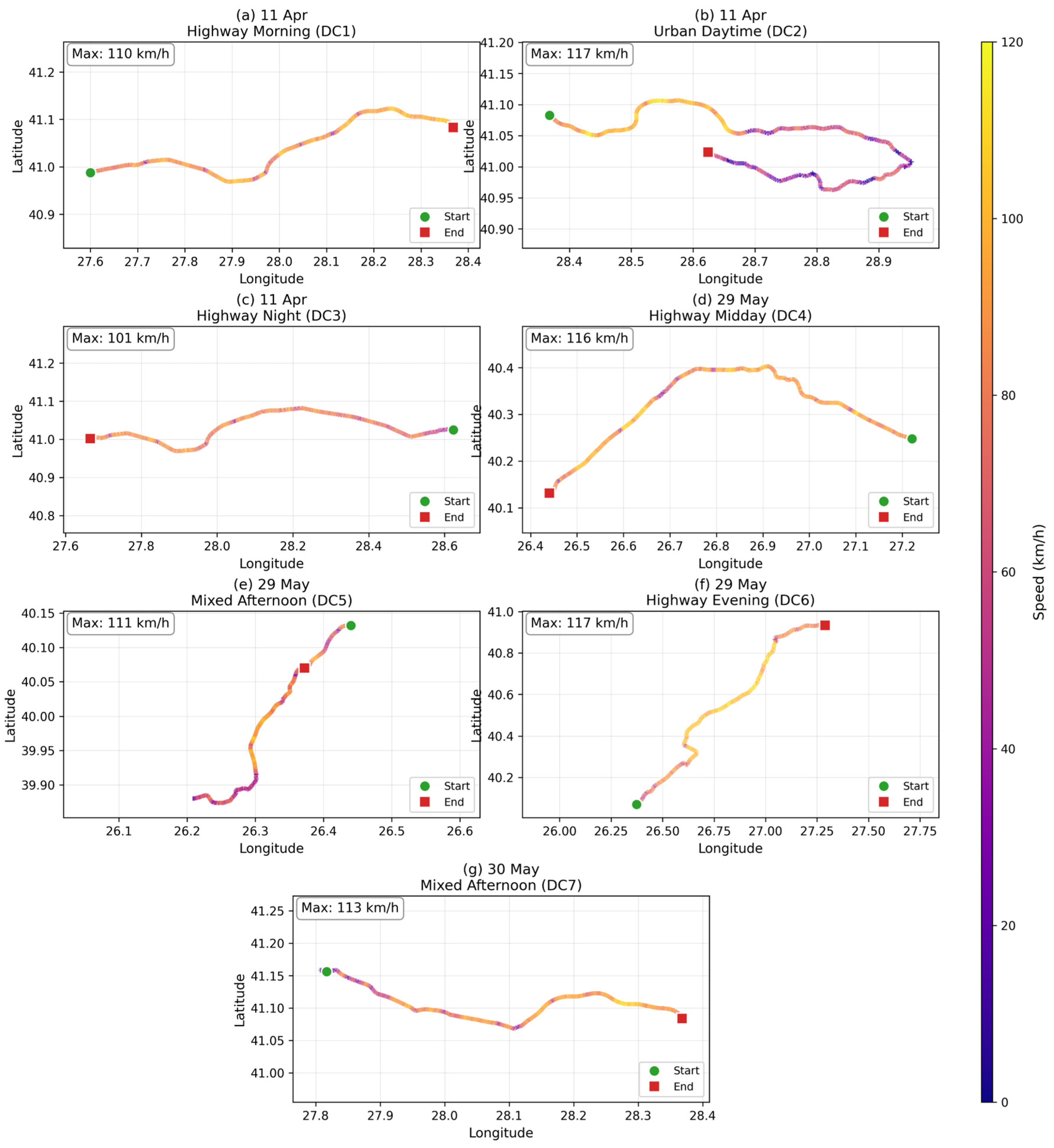
GPS route maps are presented in Figure 1. DC1 traces an eastbound motorway route from Tekirdağ (40.99° N, 27.60° E) to Silivri (41.08° N, 28.37° E) along the D-100. DC2 extends eastward from Silivri through Büyükçekmece into the inner western zones of İstanbul (reaching approximately 28.94° E, Zeytinburnu–Bağcılar area) and back, confined to the İstanbul metropolitan D-100 corridor. DC3 returns westbound along the same D-100 from the İstanbul periphery (41.03° N, 28.62° E) to Tekirdağ (41.00° N, 27.67° E), partially overlapping DC1 over the Silivri–Tekirdağ segment. DC4 follows the D-200 westbound from Biga (40.25° N, 27.22° E) to Çanakkale (40.13° N, 26.44° E). DC5 departs southward from Çanakkale along the D-550 corridor toward Ezine and returns following an extended stop. DC6 traces a northeastbound run from the Çanakkale area (40.07° N, 26.37° E) through the Gelibolu corridor to inland Tekirdağ province (40.94° N, 27.29° E). DC7 follows the D-100/E80 eastbound from Çorlu (41.16° N, 27.82° E) to the western fringe of İstanbul (41.08° N, 28.37° E). The spatial overlap of DC1 and DC3 along the D-100 enables a partial comparison of morning and night-time highway conditions over a common route; similarly, DC1 and DC7 share the Çorlu–Silivri segment, providing an April–May comparison on the same corridor.

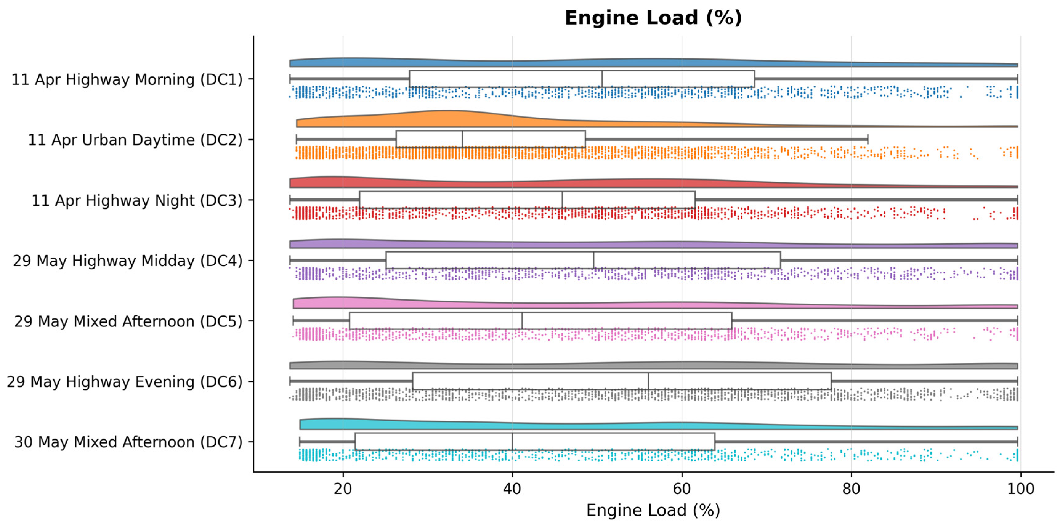
Engine load distributions broadly reflect the mechanical demands of each drive type (Figure 2). The four highway drives (DC1, DC3, DC4, DC6) show median loads in the approximate range of 45–55%, consistent with sustained partial-throttle cruising at 70–90 km/h. Among these, DC6 (Highway Evening) shows the highest median and widest upper spread, in line with its mean engine load of 55.4%—the highest across all cycles (Table 2). The distributions for the April highway runs (DC1, DC3) are slightly narrower, suggesting more uniform speed conditions, whereas the May highway runs exhibit somewhat broader spread, possibly reflecting the greater diversity of road and traffic conditions encountered on those sessions.

DC2 (Urban Daytime) shows a notably lower and more dispersed distribution, with a substantial proportion of observations concentrated at loads below 30%, corresponding to idle and low-speed urban running. Its mean engine load of 39.1% (Table 2) is the lowest among all cycles. The mixed drives (DC5, DC7) exhibit intermediate distributions: broader than the pure highway cycles but with central tendencies closer to the highway group than to DC2, consistent with a combination of arterial and open-road segments. Given the limited number of drive cycles in this study, these differences are indicative of drive-type tendencies and should not be over-interpreted.

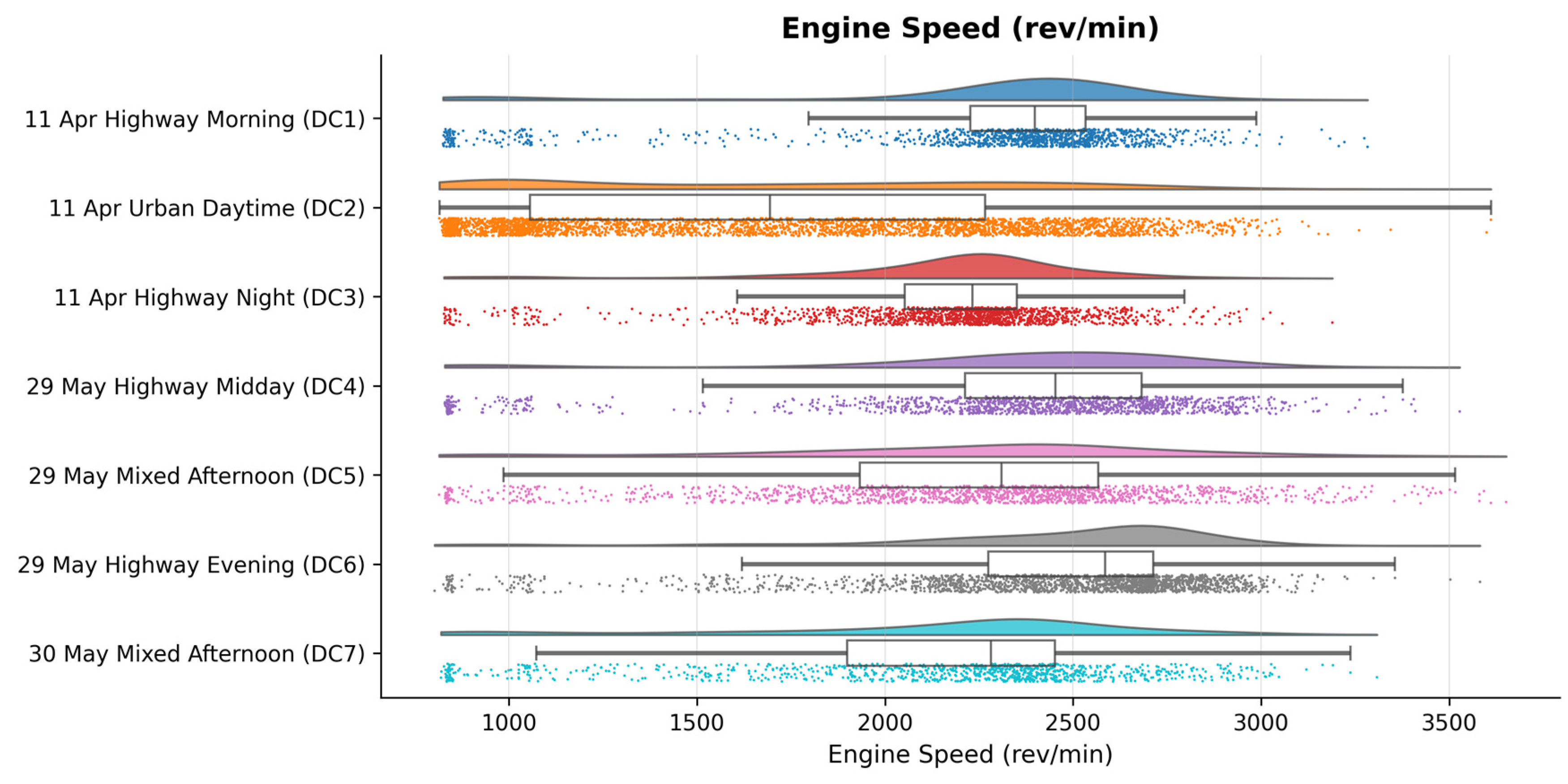
Figure 3 presents engine speed (revolutions per minute) across seven drive cycles. Engine speed distributions are closely linked to vehicle speed and gear selection. The highway drives (DC1, DC3, DC4, DC6) display concentrated distributions with medians broadly in the 2100–2450 rev/min range, corresponding to 5th or 6th gear operation at typical motorway speeds. DC6 (Highway Evening) shows the highest median, consistent with its mean RPM of 2441 rev/min (Table 2). DC3 (Highway Night) presents a slightly lower and narrower distribution compared to the daytime highway runs, which may partly reflect lower traffic density and more uniform cruising conditions.

DC2 (Urban Daytime) exhibits a markedly wider and lower distribution, with a considerable mass of observations below 1500 rev/min corresponding to idle and creeping urban traffic. Its mean of 1704 rev/min (Table 2) is the lowest recorded, and the distribution suggests frequent near-idle events consistent with stop-and-go conditions. The mixed drives (DC5, DC7) show broader distributions than the highway cycles, encompassing both low-RPM urban modes and higher-RPM open-road segments, reflecting the varied nature of their routes.

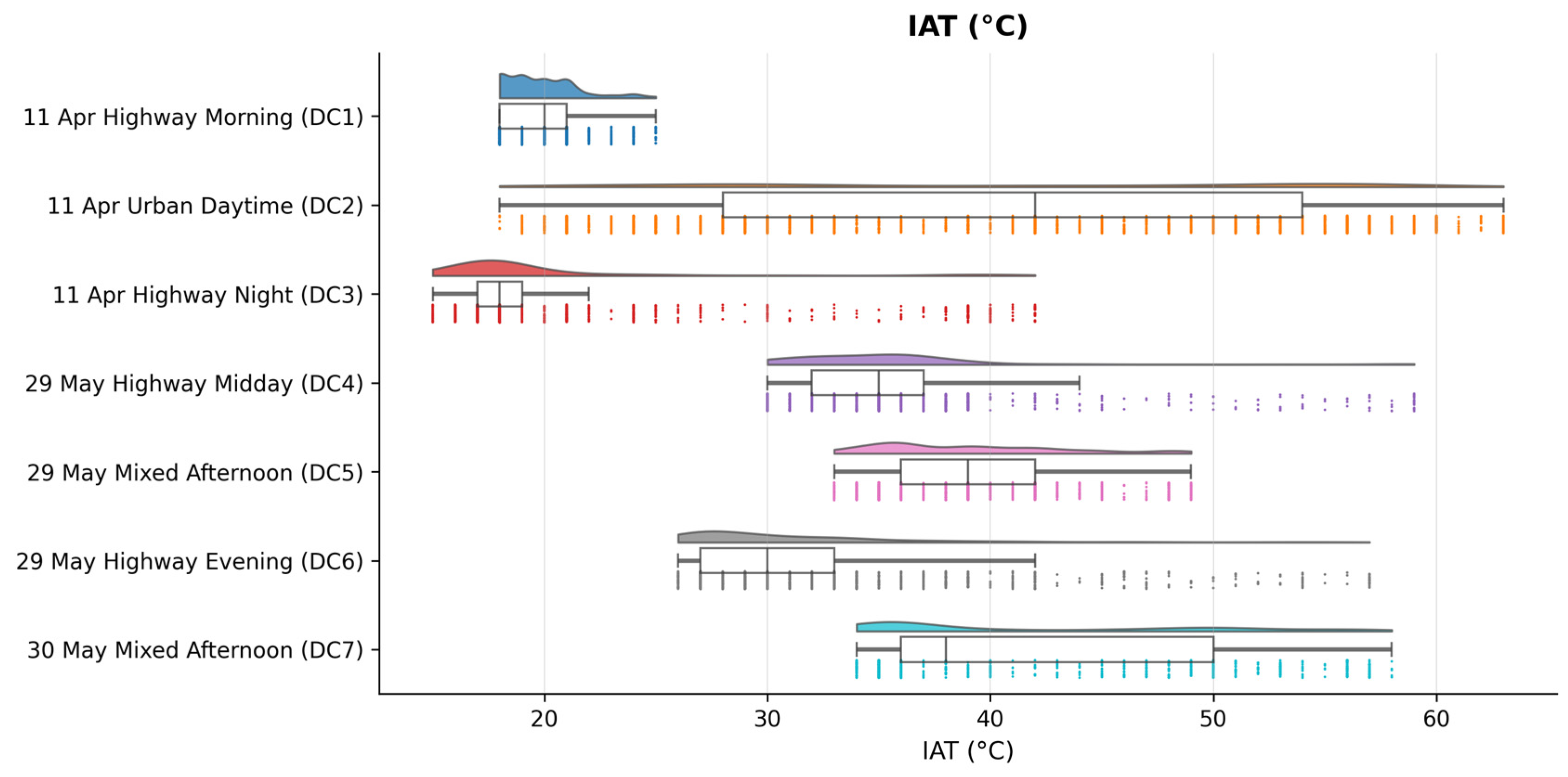
Intake air temperature distributions capture both ambient conditions and under-bonnet thermal effects accumulated during each drive (Figure 4). The two April highway drives (DC1, DC3) show narrow, low-temperature distributions with means of 19.8 °C and 20.3 °C (Table 2), consistent with cool early-spring ambient conditions. DC1 (Highway Morning) is particularly compact, with virtually all observations below 25 °C. DC3 (Highway Night) shows a slightly broader right tail, plausibly reflecting residual engine compartment heat from the preceding urban cycle.

The May drives (DC4, DC5, DC6) show substantially elevated IAT values, with means of 35.9 °C, 39.1 °C, and 31.6 °C (Table 2), reflecting warmer late-May ambient temperatures. DC6 (Highway Evening) has a somewhat lower mean than the other May drives, consistent with partial thermal relief during evening hours. DC2 (Urban Daytime) and DC7 (Mixed Afternoon, 30 May) exhibit the widest distributions with right tails reaching 63 °C and 58 °C (Table 2), respectively. The elevated peak IAT in DC2 is attributable to prolonged low-speed operation, during which reduced airflow across the engine compartment allows progressive heat accumulation. Elevated IAT reduces intake charge density, which is relevant to the higher fuel trim values observed in these same cycles (Figure 5), though the relative contribution of IAT versus other factors cannot be isolated from this dataset alone.

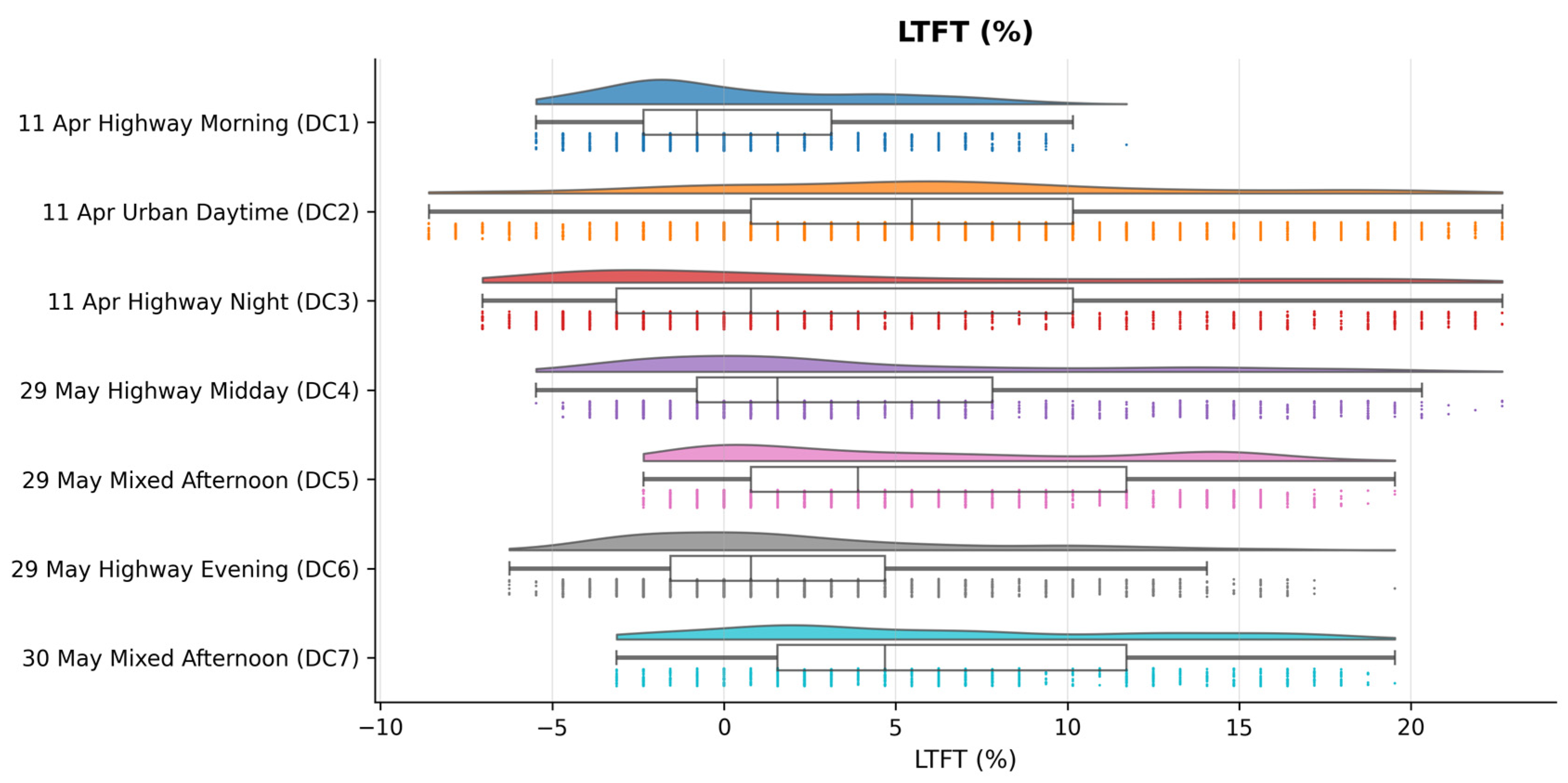
Long-term fuel trim reflects the ECU’s accumulated correction to compensate for persistent deviations from stoichiometric combustion. All seven cycles exhibit positive mean LTFT values (Table 2), indicating a systematic lean bias that the ECU corrects through enrichment. DC1 (Highway Morning) shows the lowest and most concentrated distribution, centered near +1% (mean +0.57%), suggesting near-stoichiometric learned correction under cool, steady motorway conditions. DC6 (Highway Evening) similarly shows a low central tendency (mean +2.14%).

By contrast, DC2 (Urban Daytime), DC5 (Mixed Afternoon, 29 May), and DC7 (Mixed Afternoon, 30 May) display markedly elevated distributions with means of +6.18%, +5.80%, and +6.14% respectively (Table 2), and extended right tails beyond +15%. The consistency of this elevated LTFT across different dates and routes—but similar drive types—tentatively suggests an association with low-speed, high-thermal-load operating conditions rather than a date-specific artefact, though the small number of observations precludes a firm conclusion. It should be noted that LTFT values reflect composite readings across multiple ECU operating zones encountered during each drive; the maximum recorded value of +27.34% in DC2 (Table 2) corresponds to a specific operating region (elevated temperature, low load) rather than a uniform shift across the entire fuel map (Figure 5).

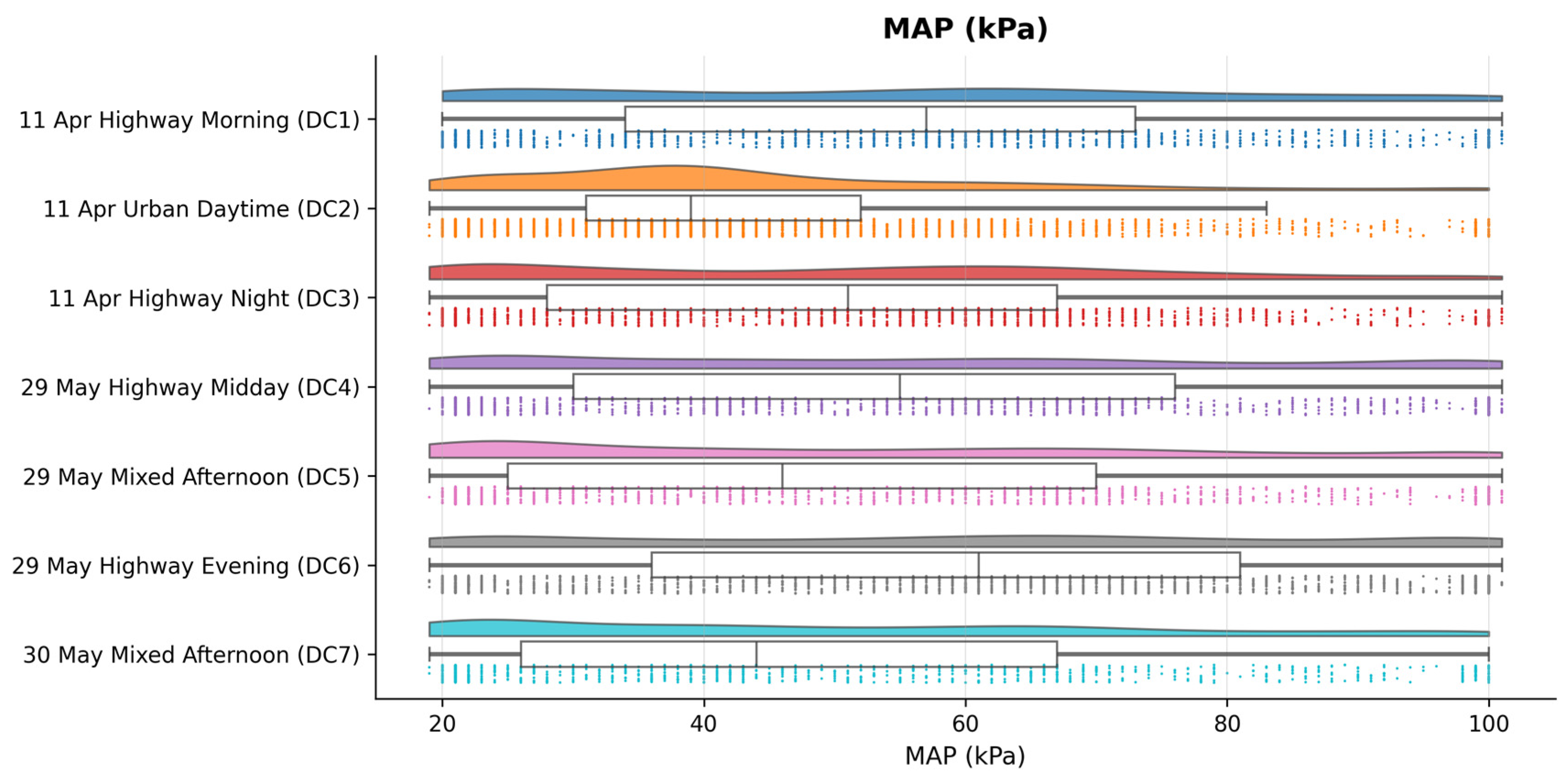
Manifold absolute pressure is a primary input to the speed-density fuel model and serves as a direct proxy for engine load: low MAP (high intake vacuum) corresponds to low-load or deceleration conditions, while high MAP (approaching atmospheric pressure, approximately 100 kPa) corresponds to high-load or full-throttle operation. The highway drives (DC1, DC3, DC4, DC6) show distributions skewed toward higher MAP values, with much of the mass concentrated between approximately 60 and 100 kPa, reflecting the sustained partial- to full-throttle demands of motorway cruising. DC6 (Highway Evening) shows the highest MAP concentration among all drives, consistent with its highest mean engine load.

DC2 (Urban Daytime) shows a notably different distribution, with greater density at lower MAP values and a wider overall spread, indicative of the frequent idle, deceleration fuel-cut, and low-load events characteristic of urban driving. The mixed drives (DC5, DC7) show intermediate distributions spanning the full range from low to high MAP, reflecting the varied throttle demands of combined urban-arterial and open-road operation. As MAP is the dominant predictor of estimated air mass in the speed-density model, its distributional differences across cycles are directly reflected in the corresponding fuel rate profiles (Figure 6).

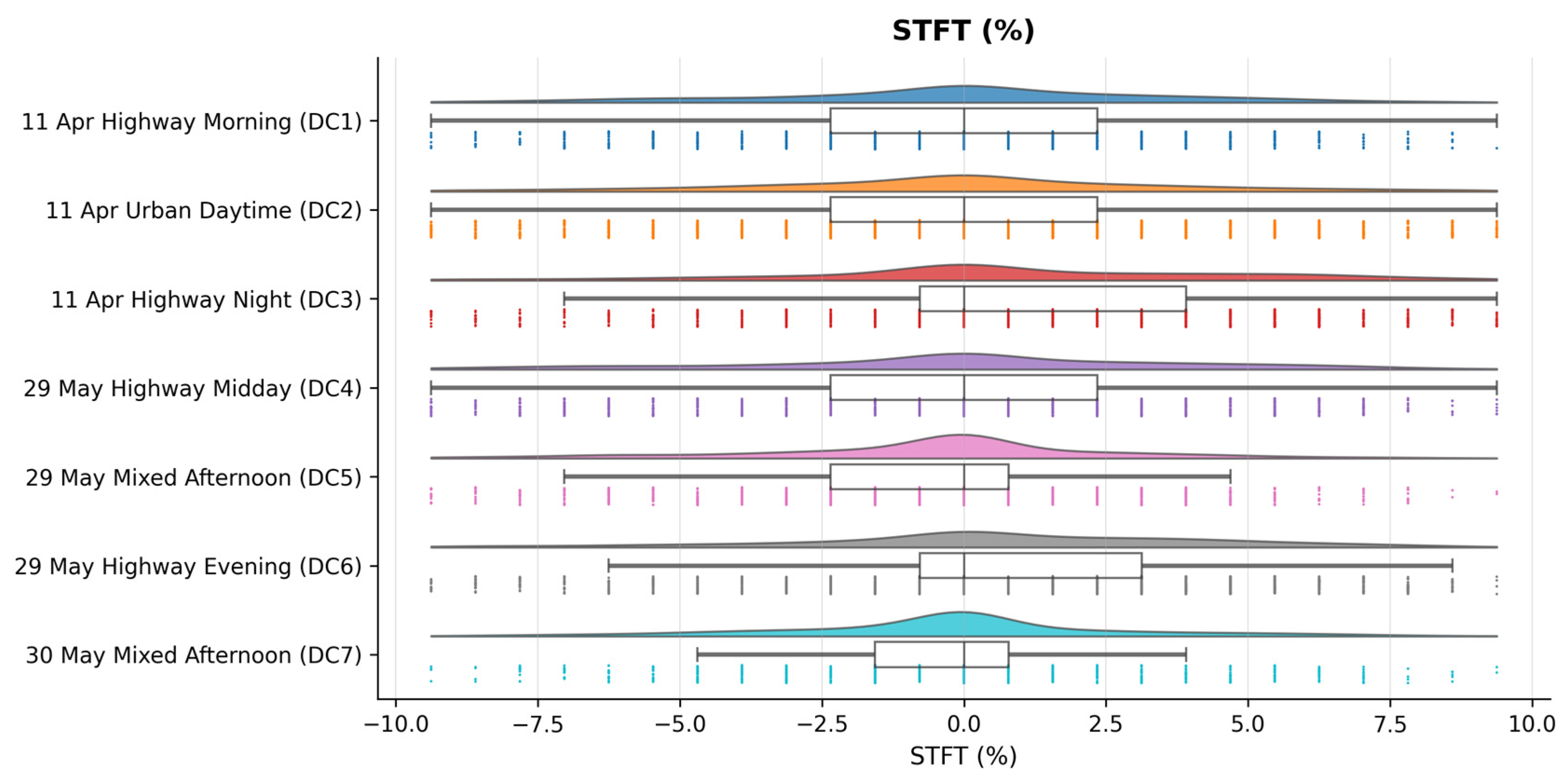
Short-term fuel trim reflects the ECU’s continuous real-time adjustment to maintain stoichiometric combustion. Unlike LTFT, which represents a learned offset, STFT fluctuates on a second-by-second basis in response to exhaust oxygen sensor readings. All seven drive cycles show distributions centered near zero, which is the expected behavior for a closed-loop fuel control system under normal operation. Mean STFT values range from −0.77% to +0.75% across cycles (Table 2), all close to zero and without a consistent directional pattern.

The interquartile ranges are broadly similar across drive types, spanning approximately ±3–5%, with tails extending to ±10% corresponding to transient throttle events. The highest recorded maximum STFT of +14.06% was observed in DC2 (Table 2), likely associated with brief fuel enrichment during aggressive urban acceleration. The overall similarity of STFT distributions across all seven cycles—in marked contrast to the substantial LTFT differences—suggests that the ECU’s real-time closed-loop control remained effective under all operating conditions tested. The modest STFT values also indicate that the speed-density model’s fuel trim correction term is primarily driven by LTFT in this dataset, rather than by short-term transient corrections (Figure 7).

3.2. Fuel Consumption Estimation and Pump Validation

Table 3. Fuel consumption comparison: speed-density model, pump fill-up (ground truth), and onboard trip computer.

Segment	Pump (L)	Model (L)	OTC (L)	Model Error %	OTC Error %
DC1	4.82	4.65	4.48	−3.6%	−7.0%
DC2	6.90	6.72	7.39	−2.7%	+7.2%
DC3	5.32	5.27	4.76	−1.0%	−10.6%
DC4	5.31	5.45	4.90	+2.6%	−7.8%
DC5	4.43	4.57	4.61	+3.2%	+4.1%
DC6	9.44	9.26	8.88	−1.9%	−5.9%
DC7	2.80	2.92	3.21	+4.3%	+14.6%
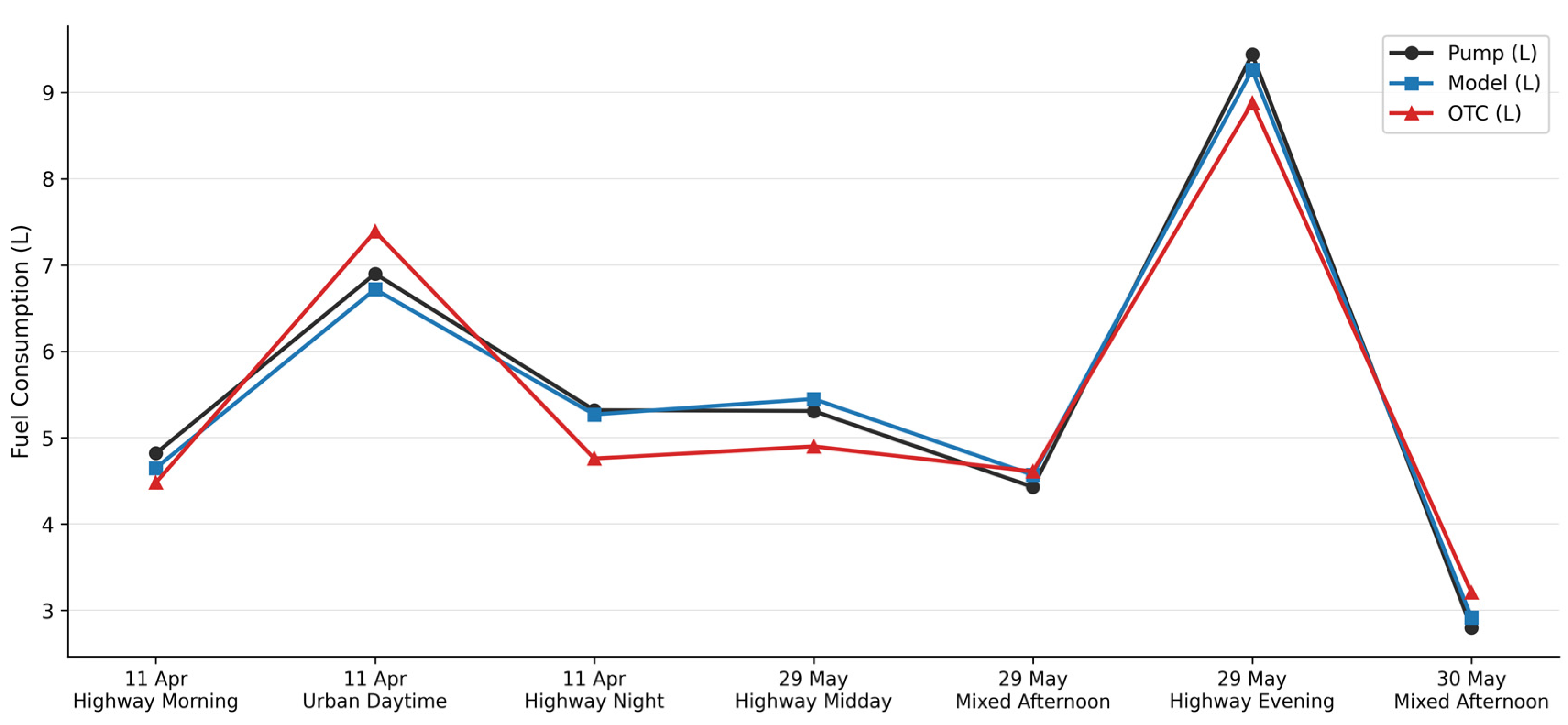
All 7 drives combined	39.02	38.83	38.24	−0.5%	−2.0%

compares speed-density model estimated fuel volumes against pump fill-up ground truth and the vehicle’s onboard trip computer across all seven drive cycles. OTC fuel volumes (L) are back-calculated from the trip computer’s displayed efficiency (L/100 km) and its own reported trip distance. All percentage errors are referenced to pump fill-up volume as the primary ground truth.

The speed-density model achieved absolute percentage errors of 3.6%, 2.7%, 1.0%, 2.6%, 3.2%, 1.9%, and 4.3% against pump measurements for DC1 through 7, respectively, corresponding to a mean absolute percentage error (MAPE) of 2.76% and a mean absolute error (MAE) of 0.14 L. Individual errors ranged from −3.6% to +4.3%, with no consistent directional bias: the three April drives (DC1–DC3) yielded small negative errors (model underestimates), whereas the May drives produced both small positive and negative deviations, indicating that the fixed volumetric efficiency assumption (ηv = 0.85) remains adequate across varying ambient temperature conditions. Across all seven drives combined (39.02 L pumped), the model total was 38.84 L, a net error of −0.5%, demonstrating good aggregate accuracy.

The onboard trip computer exhibited substantially larger and directionally inconsistent errors, with absolute values ranging from 4.1% to 14.6% (MAPE = 8.17%, MAE = 0.42 L—three times that of the speed-density model). The OTC underestimated consumption on most highway segments (DC1: −7.0%, DC3: −10.6%, DC4: −7.8%, DC6: −5.9%) while overestimating on the urban and certain mixed drives (DC2: +7.2%, DC5: +4.1%, DC7: +14.6%). This directional asymmetry suggests that OTC accuracy is drive-type dependent, consistent with reports that OTC fuel-rate algorithms are optimized for cruise conditions and underperform under transient or low-load urban operation.

Figure 8 illustrates the per-drive fuel consumption estimates for the speed-density model, pump ground truth, and onboard trip computer. The model tracks the pump reference closely across all drive types and sessions, while the OTC deviates more substantially and inconsistently.

3.3. CO₂ Footprint

Table 4. Tailpipe CO₂ footprint by drive cycle.

Segment	Pump (L)	Model (L)	CO2 Pump (kg)	CO2 Model (kg)	CO2 Intensity Pump (g/km)	CO2 Intensity Model (g/km)
DC1	4.82	4.65	11.13	10.74	152.3	146.9
DC2	6.90	6.72	15.94	15.52	170.9	166.4
DC3	5.32	5.27	12.29	12.17	140.6	139.2
DC4	5.31	5.45	12.27	12.59	141.3	145.0
DC5	4.43	4.57	10.23	10.56	141.0	145.5
DC6	9.44	9.26	21.81	21.39	153.1	150.2
DC7	2.80	2.92	6.47	6.75	119.8	125.0
All 7 drives combined	39.02	38.84	90.14	89.72	147.9	147.2

presents the tailpipe CO₂ footprint for all seven drive cycles, derived using the emission factor for gasoline combustion (EF = 2.31 kg CO₂/L). To enable a direct comparison between model-estimated and ground-truth fuel consumption, both pump fill-up volumes and speed-density model estimates are included alongside their corresponding CO₂ totals and specific intensities. OBD-integrated distance is used as the distance denominator throughout.

The pump-based and model-based CO₂ estimates are in close agreement across all seven cycles, with absolute differences in CO₂ intensity of 1–6 g/km.

CO₂ intensity varies across drive types. The urban cycle (DC2, 11 April) yields the highest intensity at 170.9 g/km (pump) and 166.4 g/km (model), approximately 16% above the mean of the four highway drives (146.8 g/km, pump). This urban CO₂ penalty is primarily attributable to the substantially lower mean speed (33.2 km/h vs. 71–85 km/h for highway drives) and the associated increase in fuel consumption per unit distance under stop-and-go conditions. Among the highway drives, DC3 (Highway Night) records the lowest intensity (140.6 g/km, pump), which may partly reflect lower ambient traffic density and more uniform cruising at night, though the single observation per cycle precludes a definitive conclusion.

DC7 (30 May Mixed Afternoon) records the lowest CO₂ intensity of all seven cycles at 119.8 g/km (pump) and 125.0 g/km (model), despite its mixed route character. This result likely reflects a combination of favorable traffic conditions on the D-100 corridor and the relatively short active duration of this cycle (51.3 min), which may not be representative of longer mixed-route operation. Accordingly, this value should be interpreted with caution.

Across all seven drives combined, the pump-based CO₂ total was 90.14 kg over 609.6 km, corresponding to a fleet-average intensity of 147.9 g/km. The model-based equivalent was 89.72 kg and 147.2 g/km—a difference in less than 1 g/km. Both values fall within the WLTP-class-equivalent range of approximately 130–150 g/km for comparable European market gasoline vehicles [1], consistent with the well-documented divergence between type-approval and real-world emissions [2,13]. The dataset is, however, drawn from a single vehicle and driver across a limited number of sessions; broader generalization requires validation across a wider range of vehicles and operating contexts.

4. Discussion

4.1. Accuracy of the Speed-Density Model

The speed-density model achieved pump-validated accuracy within ±5% across all seven drive cycles (errors −3.6% to +4.3%, MAPE = 2.76%, MAE = 0.14 L) without any vehicle-specific calibration, training data, or physical MAF sensor. Unlike the three April drives, which all yielded small negative errors, the May drives produced both positive and negative deviations, suggesting that the fixed volumetric efficiency assumption (ηv = 0.85) performs acceptably across the ambient temperature range encountered in this study rather than introducing a systematic directional bias. Comparable OBD-II-derived estimates published recently report similar error magnitudes when fixed VE values are assumed [7,8,14], and OBD-based fuel-rate studies in real traffic have reported trip-level accuracy consistent with the figures obtained here [15].

The underlying reason the method works at all without vehicle-specific calibration is that the ECU itself uses an equivalent speed-density calculation to determine fuel injection quantity. STFT/LTFT corrections continuously compensate for residual deviations between the ECU’s internal model and actual engine behavior, maintaining the post-catalyst lambda close to stoichiometry through closed-loop control [16]. By reading these corrections back over OBD-II, the external estimator inherits a large fraction of the ECU’s closed-loop accuracy—an advantage not available to open-loop models relying purely on speed or power proxies [8].

The IAT term is particularly important for atmospheric engines operating at elevated under-bonnet temperatures. DC 2’s mean IAT of 42.2 °C (peak 63 °C) represents a 7–14% reduction in air density relative to the ambient conditions of the highway cycles (mean IAT ~20 °C) [17]. If the IAT reading were ignored and a fixed reference density assumed, DC2 would be systematically overestimated by up to 15% at peak temperature. The explicit inclusion of IAT in the denominator of the speed-density equation accounts for this variation and is responsible for the model’s accuracy across thermally disparate conditions.

4.2. Comparison with the Onboard Trip Computer

Across all seven drive cycles, the OTC exhibited substantially larger and directionally inconsistent errors than the speed-density model (OTC MAPE = 8.17%, MAE = 0.42 L, range −10.6% to +14.6%; model MAPE = 2.76%, MAE = 0.14 L, range −3.6% to +4.3%). A directional pattern is apparent: the OTC underestimated consumption on all four highway drives (DC1: −7.0%, DC3: −10.6%, DC4: −7.8%, DC6: −5.9%) while overestimating on the urban and mixed drives (DC2: +7.2%, DC5: +4.1%, DC7: +14.6%). This asymmetry suggests that OTC accuracy is systematically influenced by driving regime. The highway underestimation may reflect the speed-dependent limitations of the OTC algorithm: at sustained high speeds, volumetric efficiency and injection timing deviate from the steady-state lookup tables underlying the OTC calculation, leading to systematic under-reporting. The urban and mixed overestimation may stem from incomplete accounting of low-speed and idle-period fuel use. Similar regime-dependent disparities have been documented in OBD-based engine performance studies [15], and data-driven fuel modelling reviews reach the same conclusion that single algorithms calibrated for ‘average’ cycles tend to mis-track both the low-speed and high-speed extremes [18].

The model returned better fuel consumption estimates than the OTC across all seven drive cycles. Notably, this pattern holds despite the OTC having direct access to the ECU’s internal fuel injection commands. A likely explanation is that the OTC applies temporal smoothing and display filtering to avoid rapid fluctuations in the presented value, which may introduce cumulative bias over extended drive cycles. These findings are consistent with prior work suggesting that a physics-based speed-density model, even under simplified volumetric efficiency assumptions, can achieve comparable or better trip-level accuracy relative to the manufacturer’s onboard display [7,14].

4.3. Urban CO₂ Penalty and Policy Implications

The urban drive cycle (DC2) yielded a CO₂ intensity of 170.9 g/km (pump-based), approximately 16% above the mean of the four highway drives (146.8 g/km). This urban CO₂ penalty is consistent with prior comparisons of standardized urban and extra-urban drive cycles for gasoline vehicles [19,20], and arises from the combination of lower mean speed (33.2 km/h vs. 72–85 km/h for highway drives), higher stop fraction, and more frequent acceleration events. Reviews of eco-driving research confirm that idle, stop-and-go, and aggressive acceleration phases dominate the urban-side CO₂ penalty in spark-ignition vehicles [21,22].

Across all seven drives combined, the pump-based CO₂ total was 90.14 kg over 609.6 km (147.9 g/km), with the model-based estimate differing by less than 1 g/km (147.2 g/km). Both values fall within or marginally above the WLTP-class-equivalent range of approximately 130–150 g/km for comparable European market vehicles [1], consistent with the well-documented gap between type-approval and real-world emissions [2,13]. The persistent divergence between certification and real-world fuel consumption—quantified at the fleet level as rising from approximately 8% in 2001 to roughly 40% by 2014, and remaining substantial after the NEDC-to-WLTP transition [1,23,24,25]—underscores the value of low-cost OBD-II-based field measurement methods of the type demonstrated here.

4.4. Limitations and Future Work

Several limitations should be noted. First, the study uses a single vehicle across three measurement days in a single season; generalization to other engine configurations, fuel grades, ambient temperature ranges, or driver styles is not warranted without additional validation. Driver behavior alone can shift on-road fuel consumption by 10–30% for the same vehicle and route [21]. Second, the fixed VE assumption (ηv = 0.85) is a simplification; replacing it with an RPM- and load-indexed lookup table derived from publicly available engine maps or dynamometer data for the specific engine variant would be expected to reduce residual model error [15]. Third, OBD polling at 3 s intervals is insufficient to capture transient injection events lasting tens of milliseconds; higher-frequency acquisition would improve accuracy during rapid load changes [8]. Fourth, pump fill-up volumes carry an inherent uncertainty of ±0.2% from display resolution [26].

Future work should extend validation to a fleet of vehicles encompassing turbocharged engines (where MAP-based estimation requires boost pressure correction), diesel powertrains (AFR ≈ 14.5, density ≈ 840 g/L) [7], and hybrid systems where engine-off periods complicate continuous integration. Seasonal repetition of the same routes would also quantify the sensitivity of the CO₂ footprint to ambient temperature variation, a factor known to substantially modify both criteria pollutant and CO₂ emissions in Euro 6 gasoline vehicles [27].

5. Conclusions

This study demonstrates that a physics-based speed-density model using four standard OBD-II parameters—MAP, RPM, IAT, and fuel trim corrections—achieves pump-validated fuel consumption accuracy within ±5% (errors −3.6% to +4.3%, MAPE = 2.76%) across seven drive cycles spanning highway, mixed, and urban conditions on a 1368 cm³ naturally aspirated gasoline vehicle, without a physical MAF sensor, machine learning, or vehicle-specific calibration. The intake air temperature term is essential for atmospheric engines operating under thermally varying conditions: at the peak urban under-bonnet temperature recorded (63 °C), effective air density was approximately 15% lower than under cool highway conditions, a correction that would otherwise introduce a proportional overestimation error.

The vehicle’s onboard trip computer, despite direct access to ECU injection data, exhibited substantially larger errors (MAPE = 8.17%, range −10.6% to +14.6%) with a consistent directional pattern: underestimation on highway drives and overestimation on urban and mixed drives. The speed-density model outperformed the OTC on all seven drives, confirming that OTC displays reflect user-experience filtering rather than metrological accuracy and that OBD-based physics estimates offer better trip-level fidelity.

The urban drive cycle produced a CO₂ intensity of 170.9 g/km (pump-based), approximately 16% above the mean of the four highway cycles (146.8 g/km), reflecting the fuel consumption penalty of low-speed, stop-and-go operation. The seven-drive combined intensity of 147.9 g/km (pump) is within the WLTP-class-equivalent benchmark for this vehicle class, consistent with the well-established divergence between type-approval and real-world emissions.

The methodology is reproducible using the custom Android application developed in this study, which integrates ELM327-compatible OBD-II data acquisition with concurrent smartphone GPS logging in a single unified pipeline. The application requires no additional hardware beyond a commodity Wi-Fi OBD-II adapter, making it directly deployable on the growing fleet of MAF-less vehicles and broadening the reach of low-cost emission monitoring beyond the subset of vehicles equipped with dedicated air flow sensors.

References

1. Koszałka, G.; Szczotka, A.; Suchecki, A. Comparison of fuel consumption and exhaust emissions in WLTP and NEDC procedures. Combust. Combust. Engines 2019, 179, 186–191. [Google Scholar] [CrossRef]
2. Pavlovic, J.; Anagnostopoulos, K.; Clairotte, M.; Arcidiacono, V.; Fontaras, G.; Rujas, I.P.; Morales, V.V.; Ciuffo, B. Dealing with the gap between type-approval and in-use light duty vehicles fuel consumption and CO2 emissions: Present situation and future perspective. Transp. Res. Rec. 2018, 2672, 27–37. [Google Scholar] [CrossRef]
3. Abediasl, H.; Ansari, A.; Hosseini, V.; Koch, C.R.; Shahbakhti, M. Real-time vehicular fuel consumption estimation using machine learning and on-board diagnostics data. Proc. Inst. Mech. Eng. D J. Automob. Eng. 2023, 238, 891–905. [Google Scholar] [CrossRef]
4. Tapak, P.; Kocur, M.; Matej, J. On-board fuel consumption meter field testing results. Energies 2023, 16, 6861. [Google Scholar] [CrossRef]
5. Leinonen, V.; Olin, M.; Martikainen, S.; Karjalainen, P.; Mikkonen, S. Challenges and solutions in determining dilution ratios and emission factors from chase measurements of passenger vehicles. Atmos. Meas. Tech. 2023, 16, 5075–5089. [Google Scholar] [CrossRef]
6. Nartey, D.; Alambeigi, H.; McDonald, A.D.; Shipp, E.; Manser, M.; Christensen, S.; Lenneman, J.K.; Pulver, E. A review of best practices, standards, and approaches for transportation safety data and driver state prediction. In Proceedings of the Human Factors and Ergonomics Society Annual Meeting; SAGE Publications: Los Angeles, CA, USA, 2023; Volume 67, pp. 1161–1167. [Google Scholar]
7. Malekian, R.; Moloisane, N.R.; Nair, L.; Maharaj, B.T.; Chude-Okonkwo, U.A.K. Design and implementation of a wireless OBD II fleet management system. IEEE Sens. J. 2017, 17, 1154–1164. [Google Scholar] [CrossRef]
8. Abukhalil, T.; AlMahafzah, H.; Alksasbeh, M.; Alqaralleh, B.A.Y. Fuel consumption using OBD-II and support vector machine model. J. Robot. 2020, 2020, 9450178. [Google Scholar] [CrossRef]
9. Andersson, P.; Eriksson, L. Air-to-Cylinder Observer on a Turbocharged SI-Engine with Wastegate; SAE Technical Paper 2001-01-0262; SAE International: Warrendale, PA, USA, 2001. [Google Scholar] [CrossRef]
10. Vojtíšek, M.; Kotek, M. Estimation of engine intake air mass flow using a generic speed-density method. J. Middle Eur. Constr. Des. Cars 2014, 12, 7–15. [Google Scholar] [CrossRef]
11. Oh, G.; Leblanc, D.J.; Peng, H. Vehicle energy dataset (VED), a large-scale dataset for vehicle energy consumption research. IEEE Trans. Intell. Transp. Syst. 2020, 23, 3302–3312. [Google Scholar] [CrossRef]
12. Hossain, K.R.; Rahman, M.F. Reducing the environmental impact of denim: A comparative study of green and conventional manufacturing practices. Text. Leather Rev. 2025, 8, 38–71. [Google Scholar] [CrossRef]
13. Zacharof, N.; Doulgeris, S.; Zafeiriadis, A.; Dimaratos, A.; van Gijlwijk, R.; Diaz, S.; Samaras, Z. A simulation model of the real-world fuel and energy consumption of light-duty vehicles. Front. Future Transp. 2024, 5, 1334651. [Google Scholar] [CrossRef]
14. Rykała, M.; Grzelak, M.; Rykała, Ł.; Voicu, D.; Stoica, R.-M. Modeling vehicle fuel consumption using a low-cost OBD-II interface. Energies 2023, 16, 7266. [Google Scholar] [CrossRef]
15. Rosero, F.; Rosero, X.; Mera, Z. Developing fuel efficiency and CO2 emission maps of a vehicle engine based on the On-Board Diagnostic (OBD) approach. Enfoque UTE 2024, 15, 7–15. [Google Scholar] [CrossRef]
16. Mamun, A.A.; Zhu, Q.; Hoffman, M.; Onori, S. Physics-based linear model predictive control strategy for three-way catalyst air/fuel ratio control. Proc. Inst. Mech. Eng. D J. Automob. Eng. 2021, 235, 3339–3357. [Google Scholar] [CrossRef]
17. Vaudrey, A. Thermodynamics of indirect water injection in internal combustion engines: Analysis of the fresh mixture cooling effect. Int. J. Engine Res. 2019, 20, 527–539. [Google Scholar] [CrossRef]
18. Zhao, D.; Li, H.; Hou, J.; Gong, P.; Zhong, Y.; He, W.; Fu, Z. A review of the data-driven prediction method of vehicle fuel consumption. Energies 2023, 16, 5258. [Google Scholar] [CrossRef]
19. Lim, J.-H.; Lee, Y.; Kim, K.; Lee, J. Experimental analysis of calculation of fuel consumption rate by on-road mileage in a 2.0 L gasoline-fueled passenger vehicle. Appl. Sci. 2018, 8, 2390. [Google Scholar] [CrossRef]
20. Suárez-Bertoa, R.; Valverde, V.; Clairotte, M.; Pavlovic, J.; Giechaskiel, B.; Franco, V.; Kregar, Z.; Astorga, C. On-road emissions of passenger cars beyond the boundary conditions of the real-driving emissions test. Environ. Res. 2019, 176, 108572. [Google Scholar] [CrossRef]
21. Huang, Y.; Ng, E.C.; Zhou, J.L.; Surawski, N.C.; Chan, E.F.; Hong, G. Eco-driving technology for sustainable road transport: A review. Renew. Sustain. Energy Rev. 2018, 93, 596–609. [Google Scholar] [CrossRef]
22. Lee, H.; Lee, K. Comparative evaluation of the effect of vehicle parameters on fuel consumption under NEDC and WLTP. Energies 2020, 13, 4245. [Google Scholar] [CrossRef]
23. Tietge, U.; Mock, P.; Franco, V.; Zacharof, N. From laboratory to road: Modeling the divergence between official and real-world fuel consumption and CO2 emission values in the German passenger car market for the years 2001–2014. Energy Policy 2017, 103, 212–222. [Google Scholar] [CrossRef]
24. Helmers, E.; Leitão, J.; Tietge, U.; Butler, T. CO2-equivalent emissions from European passenger vehicles in the years 1995–2015 based on real-world use: Assessing the climate benefit of the European “diesel boom”. Atmos. Environ. 2019, 198, 122–132. [Google Scholar] [CrossRef]
25. Chatzipanagi, A.; Pavlovic, J.; Ktistakis, M.A.; Komnos, D.; Fontaras, G. Evolution of European light-duty vehicle CO2 emissions based on recent certification datasets. Transp. Res. D Transp. Environ. 2022, 107, 103287. [Google Scholar] [CrossRef] [PubMed]
26. Ministry of Science, Industry and Technology. Regulation on Measuring Instruments (2014/32/EU); Official Gazette of the Republic of Turkey: Ankara, Türkiye, 2016; 29757. Available online: https://www.resmigazete.gov.tr/eskiler/2016/06/20160629-22.htm (accessed on 7 June 2026).
27. Suárez-Bertoa, R.; Astorga, C. Impact of cold temperature on Euro 6 passenger car emissions. Environ. Pollut. 2018, 234, 318–329. [Google Scholar] [CrossRef]
Figure 1. GPS route maps for the seven drive cycles, color-coded by instantaneous vehicle speed (shared plasma scale, 0–120 km/h). Panels (ag) correspond to DC1, DC2, DC3, DC4, DC5, DC6 and DC7, respectively.
Applsci 16 05879 g001
Figure 2. Engine load (%) across seven drive cycles.
Applsci 16 05879 g002
Figure 3. Engine speed (rev/min) across seven drive cycles.
Applsci 16 05879 g003
Figure 4. Intake air temperature (IAT, °C) across seven drive cycles.
Applsci 16 05879 g004
Figure 5. Long-term fuel trim (LTFT, %) across seven drive cycles.
Applsci 16 05879 g005
Figure 6. Manifold absolute pressure (MAP, kPa) across seven drive cycles.
Applsci 16 05879 g006
Figure 7. Short-term fuel trim (STFT, %) across seven drive cycles.
Applsci 16 05879 g007
Figure 8. Engine speed (RPM) versus vehicle speed (km/h) for all three drive cycles.
Applsci 16 05879 g008