AR Technology for Restoring Upper-Limb Joint Mobility in Patients

Abstract

This paper presents a comprehensive augmented reality (AR)-based rehabilitation system for upper-limb recovery that integrates AR-assisted art therapy, automated markerless goniometry, and the interval mathematical modeling of rehabilitation dynamics. The proposed platform combines four interconnected subsystems: a Python-based markerless video analysis module utilizing three stationary IP cameras, MediaPipe Pose Landmarker, and Kalman filtering; an AR art-therapy application developed for the Magic Leap 2 headset using Unity/OpenXR; a server-side subsystem implemented in NestJS/TypeScript; and a physiotherapist-oriented web application developed in React. The primary objective of the study is the real-time automated assessment of shoulder joint kinematics during AR-assisted rehabilitation sessions, including flexion (160–180°), extension (50–60°), and abduction (up to 180°). To describe and forecast rehabilitation dynamics, interval mathematical models based on recurrent difference equations were developed, enabling the prediction of subsequent joint angle values using the previous 3–4 observations. Structural and parametric identification of the interval models was performed using the artificial bee colony optimization algorithm. Experimental validation was conducted on rehabilitation data collected from five patients with different clinical diagnoses, including bursitis, epicondylitis, capsulitis, osteoarthritis, and fracture-related impairments. Under the considered experimental conditions, the proposed approach demonstrated promising predictive performance, with an angular prediction error below 5° and a correlation exceeding 95% between predicted and measured rehabilitation trajectories. The developed system implements a unified rehabilitation cycle of “execution–measurement–prediction–adaptation”, enabling the continuous monitoring of recovery dynamics, adaptive adjustment of rehabilitation scenarios, and estimation of the rehabilitation duration required to achieve target motor outcomes. The proposed approach contributes to the development of intelligent AR-based rehabilitation systems by combining markerless motion analysis, predictive interval modeling, and adaptive art-therapy mechanisms within a single clinical framework.

1. Introduction

The global demand for physical rehabilitation continues to increase due to the growing prevalence of traumatic injuries, stroke-related conditions, orthopedic and neurological disorders, and complications following surgical interventions. In Ukraine, this challenge has become particularly critical as a consequence of the full-scale war, which has resulted in a substantial increase in the number of patients with severe trauma, combined injuries and long-term functional impairments. According to the World Health Organization (WHO), within the framework of the Ukraine–WHO 2024 Health Emergency Appeal, the war has placed a significant burden on the healthcare system, with a large proportion of affected individuals requiring rehabilitation during both acute and long-term recovery phases [1]. Under such conditions, there is an urgent need for technologies capable of increasing the intensity, accessibility, and effectiveness of rehabilitation procedures without proportionally increasing the workload of healthcare personnel.

Conventional rehabilitation approaches, including kinesitherapy, therapeutic exercise, and manual rehabilitation techniques, remain fundamental components of clinical practice. However, their practical effectiveness is often constrained by several limitations, including the repetitive nature of rehabilitation exercises, patient fatigue and pain, reduced motivation, psychological exhaustion, and difficulties associated with the objective assessment of movement quality. In routine clinical settings, the evaluation of rehabilitation progress is frequently performed during short observation sessions, whereas micro-errors in movement trajectories, compensatory motions, or the instability of joint amplitudes may remain undetected. Consequently, modern rehabilitation systems require intelligent solutions capable of providing standardized rehabilitation protocols, real-time motor-oriented feedback, and automated quantitative metrics for assessing recovery dynamics.

Virtual and augmented reality (VR/AR) technologies are increasingly recognized as promising tools for clinical rehabilitation because they enable the creation of controlled interactive environments with configurable tasks, adaptive levels of complexity, and immediate visual feedback. A recent Cochrane systematic review by Laver et al. [2], updated in 2025 (5th edition; 190 studies; and 7188 participants), demonstrated that VR-based rehabilitation improves upper-limb function and activities of daily living compared to conventional therapy. Similarly, the meta-analysis conducted by Kenea et al. [3] (Journal of Clinical Medicine, 2025; 23 studies; and 395 patients) confirmed statistically significant improvements according to the Fugl–Meyer Assessment for Upper Extremities (FMA-UE) in immersive VR rehabilitation programs. Furthermore, the systematic review and meta-analysis by Plavoukou et al. [4] (Bioengineering, 2025) reported moderate-certainty evidence, according to the GRADE framework, supporting the effectiveness of VR/AR interventions for chronic musculoskeletal disorders, particularly for shoulder and upper-limb rehabilitation [5,6,7]. In upper-limb rehabilitation, VR technologies are especially relevant, because movements such as reaching, grasping, and trajectory control can be naturally integrated into interactions with virtual objects while dynamically adapting task complexity to the patient’s functional state.

A particularly promising direction is the integration of VR/AR environments with art therapy, which utilizes creative activities—including drawing, sculpting, and object manipulation—as structured therapeutic processes engaging sensorimotor coordination, motor planning, and emotional–motivational mechanisms. Art-therapy interventions influence motor recovery through several interconnected mechanisms: sensorimotor integration involving movements under continuous visual control with trajectory assessment; motor planning based on iterative cycles of “intention–action–evaluation–correction”; and emotional–motivational engagement, which reduces psychological barriers to long-term participation in rehabilitation programs [8,9]. A systematic review and meta-analysis by Joschko et al. [10] (JAMA Network Open, 2024; 50 studies; and 2766 participants) confirmed the therapeutic benefits of active visual art therapy for depression, anxiety reduction, and quality-of-life improvement. In addition, randomized clinical trials investigating VR-based art-therapy protocols demonstrated the feasibility of formalizing artistic activities as rehabilitation procedures with measurable motor outcomes [11,12].

Another important challenge in rehabilitation medicine is the prediction of rehabilitation outcomes. Accurate estimation of the number of rehabilitation sessions required to achieve normative joint mobility values is essential for treatment planning, clinical decision support, and the optimization of healthcare resources. However, existing predictive approaches, including regression-based and machine-learning models, are often limited by the heterogeneity of rehabilitation data, variability in measurement quality, and insufficient patient-specific datasets [13,14]. Under such conditions, interval data analysis methods provide an alternative mathematical framework capable of formalizing measurement uncertainty and constructing predictive intervals that remain clinically interpretable for physiotherapists and rehabilitation specialists [15,16].

The relevance of VR/AR technologies for rehabilitation medicine is determined by several factors:

–

The growing demand for rehabilitation services in Ukraine caused by the increasing number of patients with traumatic and functional impairments associated with military actions [1];

–

The necessity to improve patient motivation and rehabilitation effectiveness through controlled interactive environments incorporating art-therapy elements [5,6,7,8,9];

–

The need for the automated acquisition of kinematic data and quantitative metrics for objective progress monitoring and standardization of rehabilitation protocols [17,18];

–

The absence of integrated systems combining markerless goniometry, predictive analytics, and AR-based art therapy within a unified adaptive rehabilitation framework (a detailed comparative analysis is presented in Section 2);

–

The lack of clinically oriented solutions integrating AR-based art therapy, automated goniometry, and interval prediction into a unified “execution–measurement–prediction–adaptation” cycle.

Therefore, the development of AR-based rehabilitation systems that combine therapeutic art-oriented interaction, automated motion analysis using stationary multi-camera configurations, and predictive interval modeling represents a scientifically justified and practically important research direction for the digital transformation of modern rehabilitation medicine.

2. Analysis of VR/AR Art Therapy Systems in Rehabilitation

In this section, a systematic comparative analysis of existing VR/AR systems for upper-limb rehabilitation is conducted in order to identify the limitations of current approaches and justify the novelty of the proposed solution. The systematization of existing approaches enables the identification of three major paradigms for integrating art therapy into technology-assisted rehabilitation environments [9].

The first paradigm, referred to as imitative VR art therapy, is based on observing and reproducing artistic works in a virtual environment. Iosa et al. [19] described the so-called “Michelangelo effect,” demonstrating that participants performing VR tasks involving the imitation of an artistic drawing exhibited shorter movement trajectories and a lower subjective perception of the workload. A subsequent study by Iosa et al. [12] (Brain Sciences, 2025) further showed that aesthetic engagement and baseline motor function significantly influence therapeutic outcomes. Tieri et al. [11] extended this concept in a randomized controlled study involving 40 post-stroke patients who completed 12 VR art-therapy sessions using the Oculus Quest 2 platform. Their results demonstrated statistically significant improvements in independence, muscle strength, and a reduction in spasticity.

The second paradigm, free-form VR art therapy, involves the direct creation of artistic objects in fully immersive three-dimensional virtual environments using platforms such as Google Tilt Brush and Gravity Sketch. Although this approach provides the highest degree of creative freedom, it completely isolates the patient from the physical environment, thereby limiting clinical supervision and reducing procedural safety in rehabilitation settings.

The third paradigm, AR-based art therapy, combines creative interaction with preservation of the connection to the real-world environment. In this case, the patient continues to perceive both their own body and the physiotherapist during therapy sessions, thereby increasing safety and enabling real-time clinical supervision. This paradigm was selected in the present study as the most promising approach for upper-limb rehabilitation in clinical practice.

To determine the gap between current scientific achievements and practical clinical requirements, a comparative analysis of existing VR/AR rehabilitation systems was performed according to six criteria: movement measurement method, rehabilitation outcome prediction, VR/AR modality, integration of art therapy, physiotherapist recommendation support, and implementation of an adaptive rehabilitation cycle. The comparison results are summarized in

Table 1. Comparative analysis of existing VR/AR upper-limb rehabilitation systems.

System	Motion Measurement	Prediction	VR/AR	Art Therapy	Recommendations	Adaptive Cycle
Tieri et al. [11]	VR controller (without goniometry)	—	VR	Yes	—	—
Vidnova [20]	Depth sensor (Azure Kinect, single camera)	—	MR	Yes	Session analytics	—
RAPAEL [21]	IMU glove (wrist and finger ROM)	—	VR	—	AI-based difficulty adaptation	Partial
MindMotion GO [22]	Kinect v2 + Leap Motion	—	VR	—	—	—
Rehabotics [23]	Exoskeleton sensors	—	AR	—	—	—
Pelosi et al. [24]	Simulated kinematics	—	VR	—	RL-based target adaptation	Partial
Proposed system	3 IP cameras + MediaPipe + Kalman filtering	Interval models	AR	Yes (active + GenAI)	Yes (explainable AI + GenAI)	Yes (full cycle)

.

Tieri et al. [11] (Brain Sciences, 2024) implemented a VR art-therapy system based on the “Michelangelo effect” for 40 post-stroke patients using Oculus Quest 2. Although the system demonstrated clinical effectiveness, it does not integrate automated goniometry, since movements are tracked only through VR controllers without the quantitative measurement of joint angles. Furthermore, the system lacks predictive modeling and does not implement an adaptive rehabilitation cycle.

Vidnova (WE/AR Studio, Kyiv, Ukraine) [20] is a mixed-reality rehabilitation platform for upper-limb recovery developed in partnership with Cisco and the Ministry of Digital Transformation of Ukraine. The system combines the Magic Leap 2 headset with an external Azure Kinect depth camera for tracking joint movements. Patients perform drawing-related rehabilitation tasks in virtual environments, while physiotherapists receive biomechanical data and real-time session analytics. Functionally, Vidnova is one of the closest systems to the approach proposed in this study. However, it relies on a single depth sensor with a limited operating range (0.5–3.5 m) and sensitivity to direct sunlight, depends on the proprietary Microsoft Azure Kinect SDK (version 1.4.1), which was discontinued in 2023, and does not include mathematical prediction models or a closed-loop adaptive rehabilitation cycle.

RAPAEL Smart Glove (Neofect) [21] is a commercial VR rehabilitation platform based on a sensor-equipped glove incorporating a nine-axis inertial measurement unit (IMU), including accelerometers, gyroscopes, magnetometers, and finger flexion sensors. The system measures wrist and finger range of motion (ROM) and automatically adjusts exercise difficulty according to measured motor capabilities. AI-based algorithms recommend game-like exercises and adapt their complexity. Nevertheless, the system remains contact-based due to the glove interface, does not measure shoulder or elbow joint angles, utilizes a non-immersive screen-based interface, and does not integrate art-therapy components or long-term rehabilitation prediction.

MindMotion GO (MindMaze) [22] is an FDA-certified rehabilitation platform for post-stroke recovery. It uses Kinect v2 depth sensors for markerless body tracking and Leap Motion controllers for hand motion capture. The system provides non-immersive screen-based 3D rehabilitation exercises with biological feedback and has undergone clinical validation involving more than 300 patients in Europe. However, it lacks art-therapy functionality, predictive rehabilitation modeling, and recommendation mechanisms, while also depending on the discontinued Kinect v2 platform.

Syringas et al. [23] (Healthcare, 2025) introduced the Rehabotics system, which combines an exoskeleton glove with serious AR-based games for upper-limb rehabilitation after stroke. In a randomized pilot study involving 60 patients, the AR-plus-exoskeleton group demonstrated significant improvements according to the Ashworth Scale and Box and Block Test compared with conventional therapy. However, the system requires specialized exoskeleton hardware, does not integrate markerless goniometry, lacks predictive modeling of rehabilitation dynamics, and does not include art-therapy mechanisms.

Pelosi et al. [24] (Scientific Reports, 2024) proposed the use of reinforcement learning (Q-learning) for the adaptive optimization of VR rehabilitation environments. The RL agent dynamically modifies target locations according to kinematic parameters such as movement duration, trajectory length, and shoulder/elbow ROM. However, this work represents a simulation study involving only two test cases rather than a clinically validated rehabilitation platform. In addition, the system does not include art-therapy mechanisms and focuses primarily on short-term reward optimization rather than long-term rehabilitation trajectory prediction.

The existence of substantial research gaps is further confirmed by several recent review studies. Abedi et al. [25] (npj Digital Medicine, 2024), in a scoping review of AI applications in virtual rehabilitation, analyzed 2172 records, of which only 13 satisfied the inclusion criteria; importantly, none of the identified systems combined rehabilitation trajectory prediction with recommendation support. Senadheera et al. [26] (Sensors, 2024), in a scoping review of 704 AI-based stroke rehabilitation studies, identified four primary domains: motor impairment assessment, assisted intervention, prediction and visualization, and neuroscience-oriented applications. Their analysis confirmed the absence of closed-loop adaptive rehabilitation systems. Similarly, Quattrocelli et al. [27] (Brain Sciences, 2024) demonstrated that machine-learning models can retrospectively predict motor recovery outcomes, including FMA-UE and Barthel Index scores, based on baseline clinical features, but such approaches remain disconnected from real-time rehabilitation workflows.

Regarding markerless goniometry, Clemente et al. [28] (Sensors, 2024) demonstrated the feasibility of three-dimensional body tracking from monocular 2D video using MediaPipe Pose for telerehabilitation applications, confirming the practical applicability of webcam-based approaches as alternatives to marker-based motion capture systems. Lauman et al. [29] (Sensors, 2025) validated the camera-based MARS system for shoulder and elbow ROM assessment on a pediatric cohort (n = 65; age 5–18 years), achieving ICC = 0.993 and RMSE < 8° for most movements. García and Santos [30] (Sensors, 2025) proposed a semantic framework for transforming outputs of optical pose detectors, including YOLO Pose and MediaPipe, into clinically interpretable parameters for real-time personalized physiotherapy assessment. These studies confirm the technological maturity of markerless motion analysis approaches; however, none of the reviewed systems integrate markerless goniometry with VR/AR rehabilitation and art-therapy functionality within a unified adaptive rehabilitation framework.

The comparative analysis presented in Table 1 demonstrates that none of the existing rehabilitation systems simultaneously integrate all six considered components. In particular, limited movement measurement accuracy remains a systemic challenge across current solutions. Tieri et al. [11] do not perform quantitative goniometric assessment; Vidnova [20] relies on a single Azure Kinect depth sensor, the production of which was discontinued; RAPAEL [21] measures the range of motion only for the wrist and fingers; MindMotion GO [22] depends on the discontinued Kinect v2 platform; and Rehabotics [23] utilizes exoskeleton glove sensors.

The proposed system addresses these limitations through the use of three stationary standard-class IP cameras combined with the MediaPipe Pose Landmarker neural network detector (33 skeletal keypoints), adaptive Kalman filtering, and multi-camera triangulation. This configuration provides a clinically acceptable accuracy of approximately 3–5° for shoulder and elbow joint measurements without requiring specialized motion capture hardware. The technological maturity of markerless approaches has been confirmed in recent studies by Clemente et al. [28], who demonstrated the applicability of MediaPipe Pose for rehabilitation scenarios, and by Lauman et al. [29], who reported ICC = 0.993 and RMSE < 8° for a camera-based ROM assessment system evaluated on a pediatric cohort (n = 65).

Another critical limitation of existing systems is the absence of rehabilitation outcome prediction. None of the six analyzed platforms incorporates mathematical models for forecasting rehabilitation dynamics. Pelosi et al. [24] applied reinforcement learning for the short-term adaptation of rehabilitation scenarios; however, their approach does not address long-term recovery prediction. Quattrocelli et al. [27] demonstrated that machine-learning approaches are capable of predicting motor recovery, although only in retrospective analytical settings. Furthermore, the review studies by Abedi et al. [25] and Senadheera et al. [26] identified a substantial gap between the existence of AI-based rehabilitation methods and their integration into closed-loop adaptive rehabilitation systems.

The novelty of the proposed approach lies in the application of interval mathematical modeling of rehabilitation dynamics combined with structural and parametric identification using the artificial bee colony (ABC) algorithm. Unlike conventional data-driven predictive approaches, the proposed interval framework is capable of operating under conditions of limited clinical datasets (10–20 rehabilitation sessions), while simultaneously providing guaranteed predictive bounds for rehabilitation trajectories.

With respect to the art-therapy paradigm, Tieri et al. [11] implemented imitative VR art therapy within a fully isolated virtual environment, whereas the study by Iosa et al. [12] demonstrated that aesthetic engagement is a significant factor influencing therapeutic outcomes. Vidnova [20] supports drawing activities in mixed reality; however, it does not adapt therapeutic content to individual patient characteristics. The remaining systems (RAPAEL, MindMotion GO, Rehabotics, and Pelosi) do not include art-therapy components at all. In contrast, the proposed system implements AR-based art therapy within the third rehabilitation paradigm, preserving the patient’s connection to the real environment while simultaneously enabling the automatic generation of personalized therapeutic visual content using generative AI methods based on the patient’s biomechanical profile.

Finally, the absence of a closed-loop adaptive rehabilitation cycle is a common limitation of all analyzed systems. RAPAEL only implements a partial adaptation of exercise difficulty, while Pelosi et al. [24] demonstrated reinforcement-learning-based adaptation exclusively in simulation experiments and without transparency for decision-making mechanisms. Vidnova provides biomechanical analytics but does not support rehabilitation prediction or recommendation generation. The proposed system implements a complete adaptive rehabilitation cycle: “execution → measurement → prediction → recommendation → image correction → movement adaptation”. Importantly, each recommendation generated by the system is accompanied by quantitative justification, thereby improving interpretability and explainability for physiotherapists.

Therefore, the comparative analysis confirms that none of the existing rehabilitation systems simultaneously integrates markerless multi-camera goniometry, interval-based rehabilitation forecasting, AR-based art therapy, recommendation support, and a closed-loop adaptive rehabilitation cycle. The proposed system addresses these identified limitations by integrating all five components into a unified adaptive rehabilitation framework, which constitutes the primary scientific and technological contribution of this study.

3. Analysis of Methods for Modeling Dynamics and Predicting Rehabilitation Outcomes

A key component of any intelligent rehabilitation system is a mathematical model of recovery dynamics, which enables prediction of the trajectory of joint mobility angles based on measurements obtained during initial therapy sessions. The quality of such predictions directly determines the physiotherapist’s ability to adjust the treatment program in a timely manner. The main classes of forecasting methods used in medical applications are discussed below.

Regression analysis: This classical approach models the current value of an outcome variable as a function of independent variables such as time, previous measurements, and patient-specific clinical characteristics. Model parameters are typically estimated using the least squares method, while multiple or logistic regression is applied in dynamic settings. The main advantages include interpretability of coefficients, the ability to perform statistical significance testing (t-test, F-test), and transparency for clinicians. However, regression analysis has significant limitations: (1) the assumption of linearity is often violated in nonlinear recovery trajectories; (2) the method is sensitive to residual autocorrelation, multicollinearity, and outliers; and (3) with small sample sizes (e.g., 10–15 sessions per patient), reliable estimation of statistical characteristics becomes infeasible [31]. As a result, regression provides point estimates that fail to reflect the true uncertainty of predictions.

Autoregressive methods (AR, ARMA, and ARIMA): In these approaches, the current value of a time series is expressed as a linear combination of previous values and residual terms, with ARIMA additionally addressing non-stationarity through differencing. Their advantages include the ability to account for autocorrelation structure, interpret lag coefficients, and relatively simple implementation. However, these methods remain fundamentally linear, limiting their ability to capture acceleration or deceleration phases in recovery processes. Model order selection (p, q) requires manual tuning (e.g., using AIC/BIC criteria) and depends on data volume, while non-stationary series require preprocessing. For rehabilitation data with limited observation lengths, the Box–Jenkins methodology often produces unstable results [32].

Neural networks and deep learning methods (RNN, LSTM, and GRU): Recurrent architectures, particularly Long Short-Term Memory (LSTM) networks, which address the vanishing gradient problem through memory gating mechanisms, represent powerful tools for modeling nonlinear temporal dependencies and long-term patterns [33]. These models can automatically extract features without manual engineering and achieve high accuracy given sufficiently large datasets. However, in rehabilitation forecasting, they exhibit critical limitations: (1) “black-box” nature, resulting in low interpretability for clinicians who require an understanding of the prediction logic; (2) the need for large datasets to avoid overfitting—given only 10–15 measurements per patient, LSTM models are prone to overfitting [34]; and (3) high computational complexity, which complicates deployment in clinical environments.

Justification of the interval-based approach: All of the above methods share a fundamental limitation: they operate on point-valued measurements and ignore uncertainty, which is inherent in markerless video-based goniometry (e.g., detection errors, occlusions, and lighting variations). Instead of masking measurement errors as precise values, it is more appropriate to represent joint angle measurements as intervals with bounded uncertainty and to construct discrete dynamic models using interval analysis methods. This approach offers several advantages:

(1)

Natural handling of noise and missing data—wider intervals are formed where measurement quality is lower and narrower ones where it is higher;

(2)

Prediction results are expressed as intervals rather than point estimates, inherently providing a quantitative measure of reliability that is interpretable for clinicians;

(3)

Model parameters can be identified even with small datasets, avoiding the overfitting typical of neural network approaches [15,16].

This aligns with contemporary requirements for transparency and methodological rigor in clinical predictive modeling, reinforced by international reporting standards and risk-of-bias assessment frameworks [35,36].

Thus, among the considered approaches, interval data analysis methods most comprehensively address the specific characteristics of rehabilitation time series, including the handling of small and noisy datasets, the need for interpretable predictions, and the ability to explicitly formalize uncertainty within the measurement subsystem.

4. Authors’ Previous Developments as the Basis for the Study

The study presented above represents a direct continuation of a series of prior works by the authors, in which individual components of a comprehensive clinical AR-based rehabilitation system were progressively developed.

In the first stage, a software system supporting art-therapy processes based on augmented reality technologies was developed and validated [37]. The system was implemented on the Magic Leap 2 headset using Unity/OpenXR, providing a spatially anchored AR drawing interface under the direct supervision of a physiotherapist in a clinical environment. This work confirmed the technical feasibility of the AR-based approach for art therapy sessions and, at the same time, revealed a critical limitation, the absence of an objective automated measurement of joint mobility angles, which is essential for the quantitative evaluation of therapy effectiveness.

At the second stage, to address this limitation, the authors developed an innovative web-based goniometric analysis system [37] and an automated neural network-based goniometric analysis system [38]. Both systems enable the markerless real-time measurement of upper-limb joint angles using neural network-based keypoint detection, thereby eliminating the subjectivity of manual goniometry and allowing the acquisition of standardized kinematic data during each session. However, these systems relied on a single-camera configuration, which limited measurement accuracy due to projection errors under unfavorable viewing angles.

Thus, the previous studies established two key components of the system: the AR-based art therapy environment and the automated goniometric analysis subsystem. The identified limitations—namely, the absence of a prediction module and the use of a single-camera configuration—form the direct motivation for the present study. The proposed approach integrates and extends previous developments by introducing the following:

(1)

A three-camera configuration combined with an adaptive Kalman filter to reduce projection errors;

(2)

An interval-based mathematical modeling and prediction module for recovery dynamics, thereby completing the full “execution–measurement–prediction–adaptation” cycle within a unified clinical system.

5. System Architecture

The developed system is a comprehensive hardware–software solution for clinical AR-based upper-limb rehabilitation designed to operate in a controlled rehabilitation room environment under the direct supervision of a physiotherapist. It extends previously validated components developed by the authors—namely, an AR-based art therapy application for Magic Leap 2 [37] and a neural network-based automated goniometric analysis subsystem [37,38]—by integrating them into a unified architecture with a three-camera markerless joint angle measurement module and an interval-based prediction component.

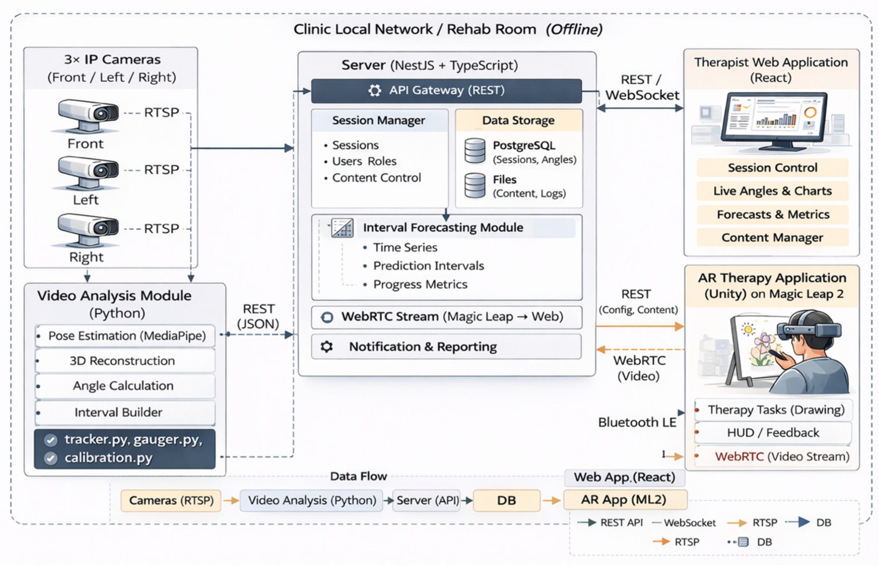
The system consists of four interconnected subsystems, illustrated in Figure 1.

-

A Python-based (version 3.11.12) markerless video analysis subsystem utilizing three stationary IP cameras;

-

An AR application for the Magic Leap 2 headset developed using the Unity engine;

-

A server-side component implemented in NestJS/TypeScript;

-

A physiotherapist web application developed using React.

All components are deployed within the local network of the rehabilitation room; none of the subsystems require external Internet connectivity during operation.

The overall workflow of a clinical session is organized as follows. The physiotherapist initiates the session via the web application and configures the AR scene (environment, canvas geometry, and therapeutic image). The patient then wears the Magic Leap 2 headset and performs the art therapy task—drawing in the AR space using hand gestures. Simultaneously, three IP cameras capture limb movements in real time. The Python-based subsystem computes joint mobility angles and transmits the data via the NestJS server to the web interface. The physiotherapist monitors kinematic data and the live video stream from the headset (via WebRTC) and can dynamically adjust session parameters. After the session, the recorded time series of joint angle measurements are stored for subsequent interval-based modeling and the prediction of recovery dynamics.

5.1. Python-Based Markerless Video Analysis Subsystem

Hardware Configuration: Three IP cameras are installed in fixed positions within the rehabilitation room at mutually perpendicular viewpoints relative to the patient’s working area: FRONT (frontal view), LEFT, and RIGHT (lateral oblique side views). This arrangement ensures that, for each of the primary movements of the shoulder, elbow, and wrist joints, at least one camera is positioned close to the plane of motion (deviation angle φ < 20°), thereby limiting the projection error to 3–5° [39]. The cameras are assigned static IP addresses within the 192.168.1.0/24 subnet, and video streams are transmitted via RTSP/TCP (RTP/TCP, RFC 2326 [40,41]) to ensure reliable delivery within the local network.

The joints.py Module: Anatomical Definitions: The MediaPipe Pose Landmarker neural network detector [41,42] returns an array of 33 normalized anatomical landmark coordinates ($x,y,z\in [0,1]$; visibility confidence $\in [0,1]$). The joints.py module defines the POSE_IDX dictionary, which maps semantic landmark names (e.g., L_SHOULDER, R_ELBOW) to numerical indices, as well as a set of JointAngleDef structures. Each structure describes a single angular parameter: point_a (proximal point), vertex (joint vertex), point_b (distal point), norm_min/norm_max (range-of-motion norms according to AAOS standards [43]), and the calculation metric (‘direct’ or ‘from_straight’). In total, 11 parameters are defined for each side of the body (22 parameters overall), covering six shoulder joint movements, four elbow joint movements, and one wrist joint movement (

Table 2. Angular parameters of the system (per body side; 22 parameters in total).

Parameter	Point_a	Vertex	Point_b	Norm (°)	Metric
Shoulder: flexion	Hip	Shoulder	Elbow	160–180	direct
Shoulder: extension	Hip	Shoulder	Elbow	50–60	direct
Shoulder: abduction	Elbow	Shoulder	opp_Shoulder	180	direct
Shoulder: adduction	Hip	Shoulder	Elbow	30	direct
Elbow: flexion	Shoulder	Elbow	Wrist	140–160	from_straight
Elbow: hyperextension	Shoulder	Elbow	Wrist	8–12	from_straight
Elbow: pronation	Shoulder	Elbow	Wrist	85–95	direct
Elbow: supination	Shoulder	Elbow	Wrist	85–90	direct
Wrist: flexion	Elbow	Wrist	HAND_AXIS	70–80	from_straight
Wrist: extension	Elbow	Wrist	HAND_AXIS	60–70	from_straight

).

The tracker.py Module: Detection and Angle Computation: The PoseTracker class loads the TFLite model pose_landmarker_full.task (full version of BlazePose [41]) in VIDEO mode, which ensures temporal coherence between consecutive frames through internal track association across inference calls. Prior to neural network inference, frame resizing to INFERENCE_MAX_SIDE = 640 px reduces the computational load by approximately 2–4× without significant loss of the detection accuracy for 1280 × 720 video streams.

In contrast to the previously developed single-camera web-based goniometric analysis system [37,38], which relied on a single frontal-view camera, the current implementation processes stream from three cameras in parallel using separate threads. This significantly extends the coverage of movement planes and improves the robustness of joint angle estimation.

The HandTracker module additionally detects 21 hand keypoints using the hand_landmarker.task model. The assignment of left/right hands is performed by minimizing the Euclidean distance to the corresponding wrist landmarks obtained from the pose model.

The CombinedTracker module integrates both detectors, applying hand detection on every second frame (HAND_DETECT_EVERY_N = 2) to optimize CPU utilization. This approach allows for maintaining the total processor load below 80% while processing three video streams simultaneously.

The calibration.py Module: Adaptive Kalman Filtering: For each anatomical landmark, an independent instance of the KalmanLandmark class is maintained, with the state vector x_k = [p_x, p_γ, v_x, v_γ]^T representing spatial coordinates and their temporal derivatives (velocities). A constant-velocity kinematic model is employed, with the state transition matrix F ∈ ${\mathbb{R}}^{4\times 4}$ and the observation matrix H ∈ ${\mathbb{R}}^{2\times 4}$. The standard Kalman prediction and update steps [44,45] are given by:

$${\widehat{\mathbf{x}}}_{k|k-1}=F·{\widehat{\mathbf{x}}}_{k-1|k-1}, P_{k|k-1}=F·P_{k-1|k-1}·F^{\top }+Q$$

(1)

$$\begin{gathered} K_k=P_{k|k-1}·H^{\top }·S_k^{-1}, {\widehat{\mathbf{x}}}_{k|k}={\widehat{\mathbf{x}}}_{k|k-1}+K_k·\left({\mathbf{z}}_k-H·{\widehat{\mathbf{x}}}_{k|k-1}\right), \\ {P}_{k|k}=\left(I_4-K_k·H\right)·P_{k|k-1} \end{gathered}$$

(2)

Innovation Gate: The classical Kalman filter with a fixed measurement noise covariance R produces suboptimal results: a small R leads to instability under detection outliers, whereas a large R results in the excessive smoothing of rapid movements. To address this trade-off, an adaptive measurement noise parameter $r_k$ is introduced based on the Euclidean norm of the innovation $d_k={‖{\mathit{z}}_k-H·{\widehat{\mathit{x}}}_{k|k-1}‖}_2:$

$$r_k=\left\{\begin{array}{ll}{r}_{base},& if{ d}_k\le gate\\ r_{base}·{\left({\displaystyle \frac{gate}{d_k}}\right)}^2,& if d_k>gate\end{array}\right. gate=35 px,$$

(3)

where $\mathrm{g}\mathrm{a}\mathrm{t}\mathrm{e}=35 \mathrm{p}\mathrm{x}$ denotes the innovation gate threshold. The quadratic dependence ensures smooth adaptation: for example, when $\mathrm{g}\mathrm{a}\mathrm{t}\mathrm{e}=35 \mathrm{p}\mathrm{x}$ denotes the innovation gate threshold. The quadratic dependence ensures a smooth reduction in the measurement noise covariance $R$ during rapid movements: for $d_k=2·\mathrm{g}\mathrm{a}\mathrm{t}\mathrm{e}\to$ $r_k=r_{\mathrm{b}\mathrm{a}\mathrm{s}\mathrm{e}}/4$; for $d_k=3·\mathrm{g}\mathrm{a}\mathrm{t}\mathrm{e}\to$ $r_k=r_{\mathrm{b}\mathrm{a}\mathrm{s}\mathrm{e}}/9$.

Warm-Up Schedule: At the beginning of a session, the state vector is not yet initialized (“cold start”), which leads to instability in the initial measurements. To mitigate this effect, a linear interpolation of $r_{\mathrm{b}\mathrm{a}\mathrm{s}\mathrm{e}}$ is applied from $r_{\mathrm{h}\mathrm{i}\mathrm{g}\mathrm{h}}=0.35$ to $r_{\mathrm{s}\mathrm{t}\mathrm{a}\mathrm{b}\mathrm{l}\mathrm{e}}=0.06$ over $\mathrm{W}\mathrm{A}\mathrm{R}\mathrm{M}\mathrm{U}\mathrm{P}\_\mathrm{F}\mathrm{R}\mathrm{A}\mathrm{M}\mathrm{E}\mathrm{S}=45$ frames (approximately $1.5$ s at $30$ FPS):

$$t=min\left(1.0,{\displaystyle \frac{frame\_count}{WARMUP\_FRAMES}}\right), r_{base}=r_{high}+\left(r_{stable}-r_{high}\right)·t$$

(4)

The multi_camera.py Module: Geometric Fusion of Measurements: The build_point_map_multi() function constructs a dictionary of the form $\{\mathrm{p}\mathrm{o}\mathrm{i}\mathrm{n}\mathrm{t}\_\mathrm{n}\mathrm{a}\mathrm{m}\mathrm{e}:(\mathrm{c}\mathrm{a}\mathrm{m}\mathrm{e}\mathrm{r}\mathrm{a},\mathrm{c}\mathrm{o}\mathrm{o}\mathrm{r}\mathrm{d}\mathrm{i}\mathrm{n}\mathrm{a}\mathrm{t}\mathrm{e}\mathrm{s}\left)\right\}$, selecting for each anatomical landmark the camera with the highest confidence visibility among the three available sources. The select_best_angle_sources() algorithm implements a deterministic prioritization heuristic: For movements in the frontal plane, the FRONT camera is used; for movements in the sagittal plane, the lateral camera on the side of the examined limb is selected. The joint angle is computed using a vector-based method: $ba=p_a-p_b$, $bc=p_c-p_b$, $\theta =arccos\left({\displaystyle \frac{ba·bc}{\parallel ba\parallel ·\parallel bc\parallel }}\right)$. This approach extends the previously developed single-camera automated goniometric analysis system [38], where projection error under unfavorable viewpoints reached 30–50°. The proposed three-camera configuration with geometric fusion reduces this error to 3–5° [39].

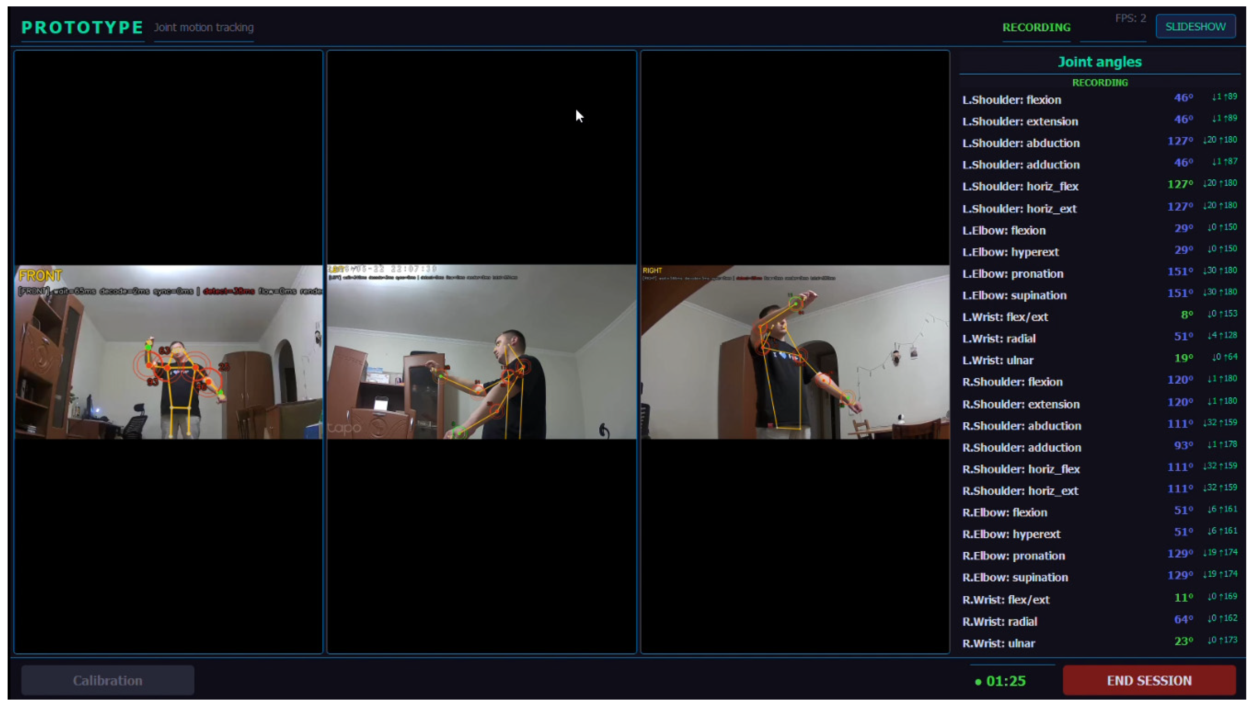
Multithreaded Architecture and Data Logging: The CameraWorker class encapsulates the full processing pipeline for a single camera (RTSP → detection → filtering → angle computation) within a dedicated Python daemon thread. Three independent threads process video streams in parallel, while synchronization of the results in the PyQt5 GUI thread is ensured atomically using threading.Lock. A QTimer with an interval of 33 ms (approximately 30 FPS) triggers interface updates and the transmission of current joint angle values to the server.

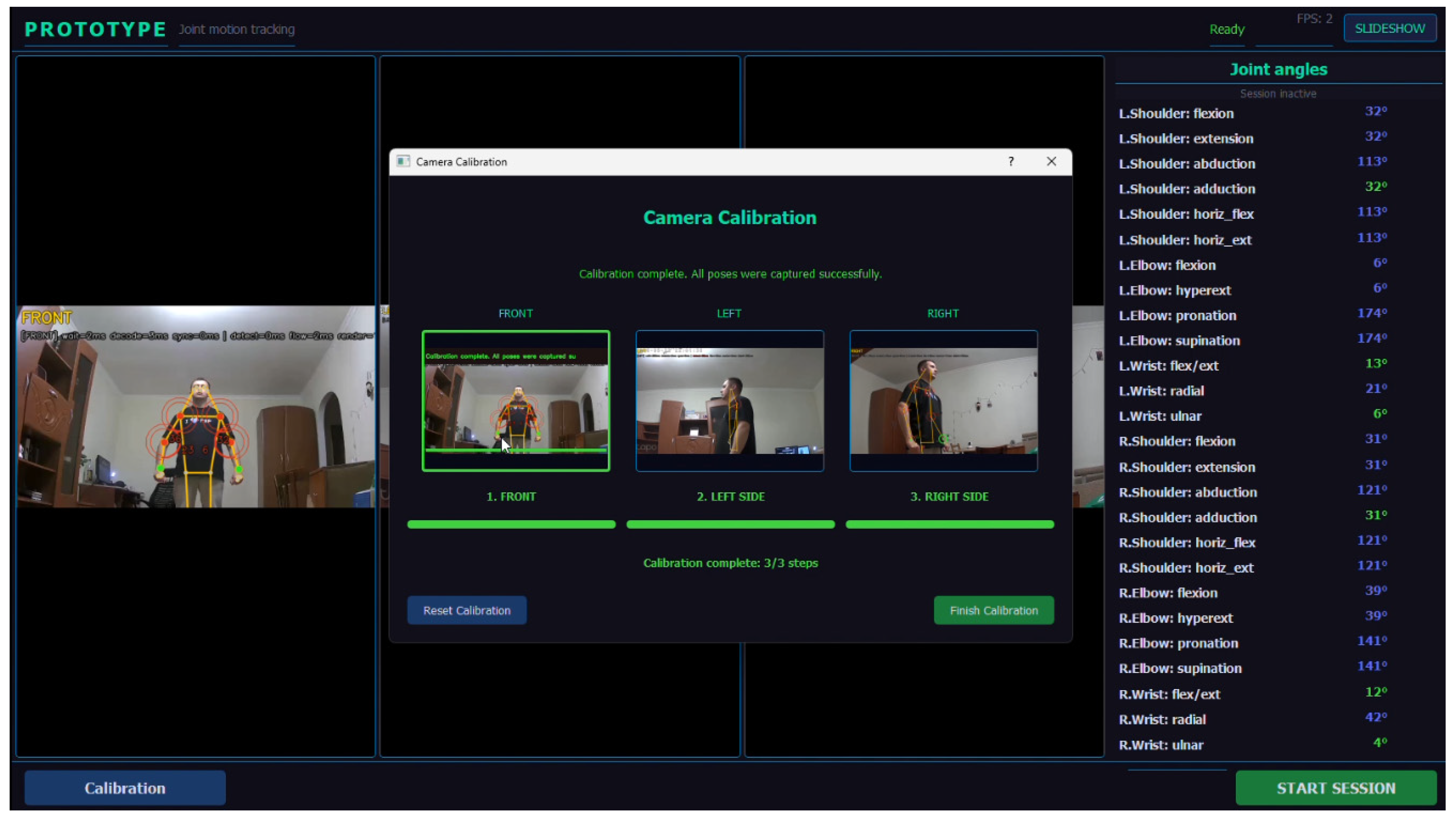
The SessionAngleLogger class records up to approximately 9000 frames of angular measurements during a 5 min session in JSON format, ensuring data integrity via a forced flush operation after each frame. The prototype interface of the video analysis subsystem is presented in Figure 2 and Figure 3: the calibration procedure for the three-camera setup (Figure 2) and the real-time joint angle detection results (Figure 3).

5.2. Unity Application for the Magic Leap 2 Headset

The AR application is implemented using the Unity 2022.3 LTS engine with an OpenXR backend for the Magic Leap 2 headset [46,47] and represents an extension of the prototype validated in the authors’ previous work [38]. Compared to the initial prototype, the current version introduces several improvements: integration with a NestJS backend for the dynamic loading of session parameters and therapeutic images from the physiotherapist’s web application; WebRTC-based video streaming for real-time clinical observation; an enhanced haptic compensation algorithm in the BrushManager; and correction of brush deformation in the TexturePainter. The subsystem consists of three key modules: WorkspaceInitializer, BrushManager, and TexturePainter.

Spatial Positioning (WorkspaceInitializer): At the start of a session, a coroutine with a 3 s delay allows the headset sensors to complete spatial mapping of the environment. The module then captures the patient’s gaze vector, projects it onto the horizontal plane, and places the WorkSpace object along this vector at a distance of 0.75 m from the patient. A critical aspect is the correction of the Pivot Offset, ensuring that the interactive canvas is centered along the gaze vector rather than at the geometric center of the composite object. This positioning guarantees an ergonomically appropriate hand posture during drawing, remaining within the therapeutic range of motion.

Haptic Compensation (BrushManager): Since AR holograms lack physical resistance, the patient’s hand may unintentionally pass through the virtual canvas, resulting in a “penetration effect.” The BrushManager module addresses this issue using a retrospective ray tracing approach: the ray origin is shifted backward by rayOffsetBack = 0.05 m relative to the index fingertip (XRHandJointID.IndexTip). Bitmask-based LayerMask configurations are used to differentiate interactions between the uiLayer and drawingLayer.

Texture Rendering (TexturePainter): Drawing is implemented through the direct manipulation of the texture pixel array using the SetPixel method. An automatic brush deformation compensation mechanism is applied: rangeX = radius · max(aspectRatio, 1.0), where aspectRatio = width/height. Pixel inclusion within the brush area is determined using the circular condition: dx² + dy² ≤ radiusSq. This approach remains computationally efficient for the textures of 1024 × 1024 sized pixels.

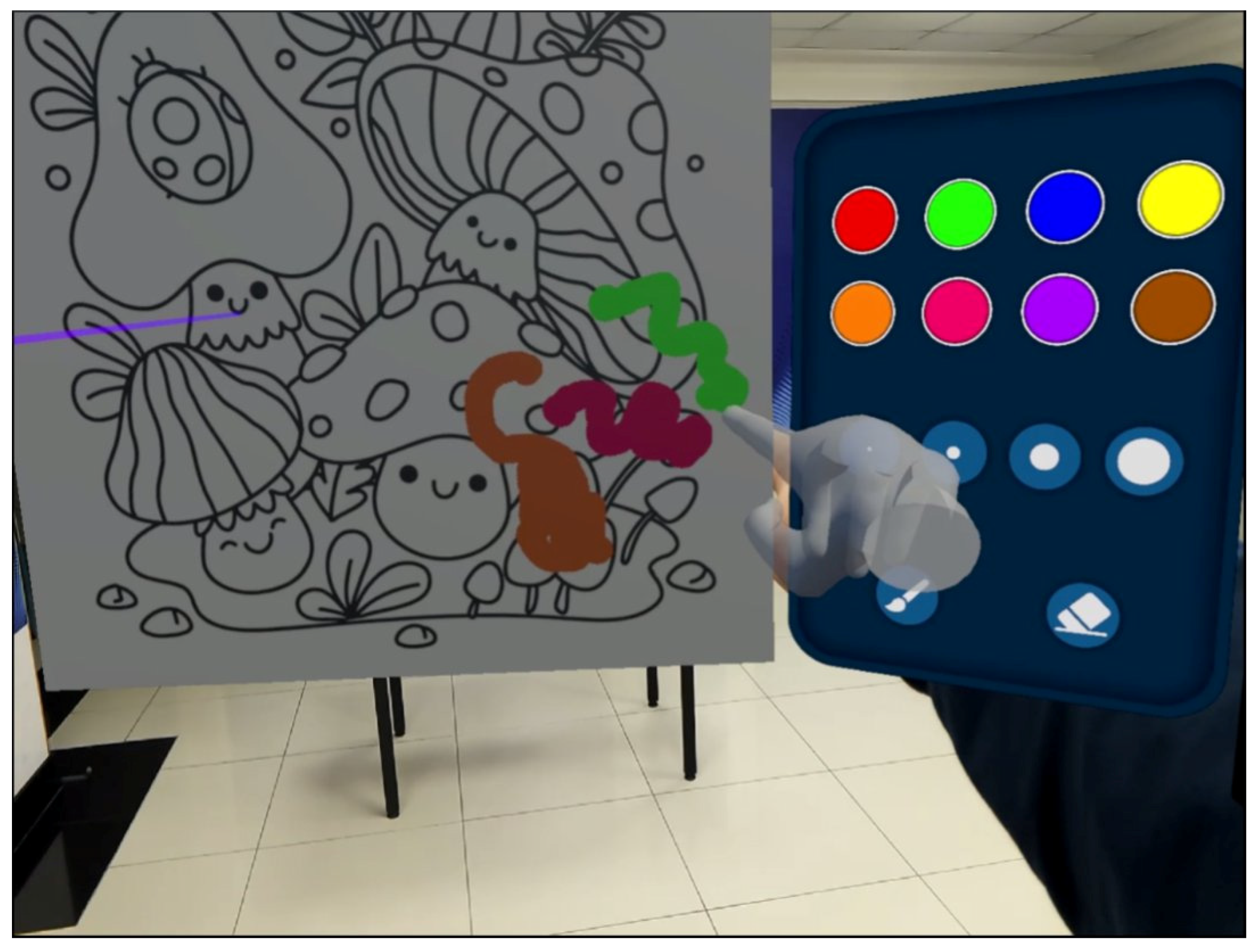
Remote Control and WebRTC Streaming: Upon initialization, the application retrieves a session configuration package from the NestJS server. Any modifications introduced by the physiotherapist are immediately reflected in the headset without requiring a restart. The Magic Leap 2 device streams video from the built-in RGB camera (1920 × 1080, 30 fps, H.264 Baseline) with AR overlays of the hand skeleton to the physiotherapist’s web interface. The end-to-end latency is approximately 60 ms. A screenshot of the AR-based art therapy interface running on the Magic Leap 2 headset is presented in Figure 4.

5.3. Server-Side Component (NestJS/TypeScript)

The server-side component is implemented using the NestJS framework [48] with TypeScript, following a layered architecture and strict separation of concerns across the Controller, Service, and Repository layers. The modular structure includes: AppModule (root module), ImageModule (media file management), HealthModule (monitoring endpoint GET/health), and WebRtcModule (WebRTC signaling via Socket.IO). Three global providers are configured: ValidationPipe with whitelist and forbidNonWhitelisted modes; HttpExceptionFilter for centralized error handling; and ResponseInterceptor, which standardizes the JSON response format as $\{success, statusCode, data, timestamp\}$.

WebRTC Signaling and Session Management: The WebRtcModule implements a signaling gateway to establish a direct peer-to-peer WebRTC connection between the headset and the physiotherapist’s browser. The protocol operates as follows: (1) POST/api/v1/rooms—the server returns a unique roomId; (2) the headset connects via WebSocket; (3) exchange of SDP offer/answer and ICE candidates; and (4) establishment of a P2P DTLS-SRTP channel [49]. The RoomService class manages session lifecycle states using a Map < string, RoomSession > structure, following the state transition cycle: WAITING → ACTIVE → CLOSED.

5.4. Physiotherapist Web Application (React)

The web application is developed using React 19 with TypeScript 5.9 and built with Vite 7 (SWC compiler written in Rust, reducing build time by approximately 5–10×). No external UI libraries are used; navigation between three main screens is implemented via an internal state variable: ‘overview’|registration|’session’.

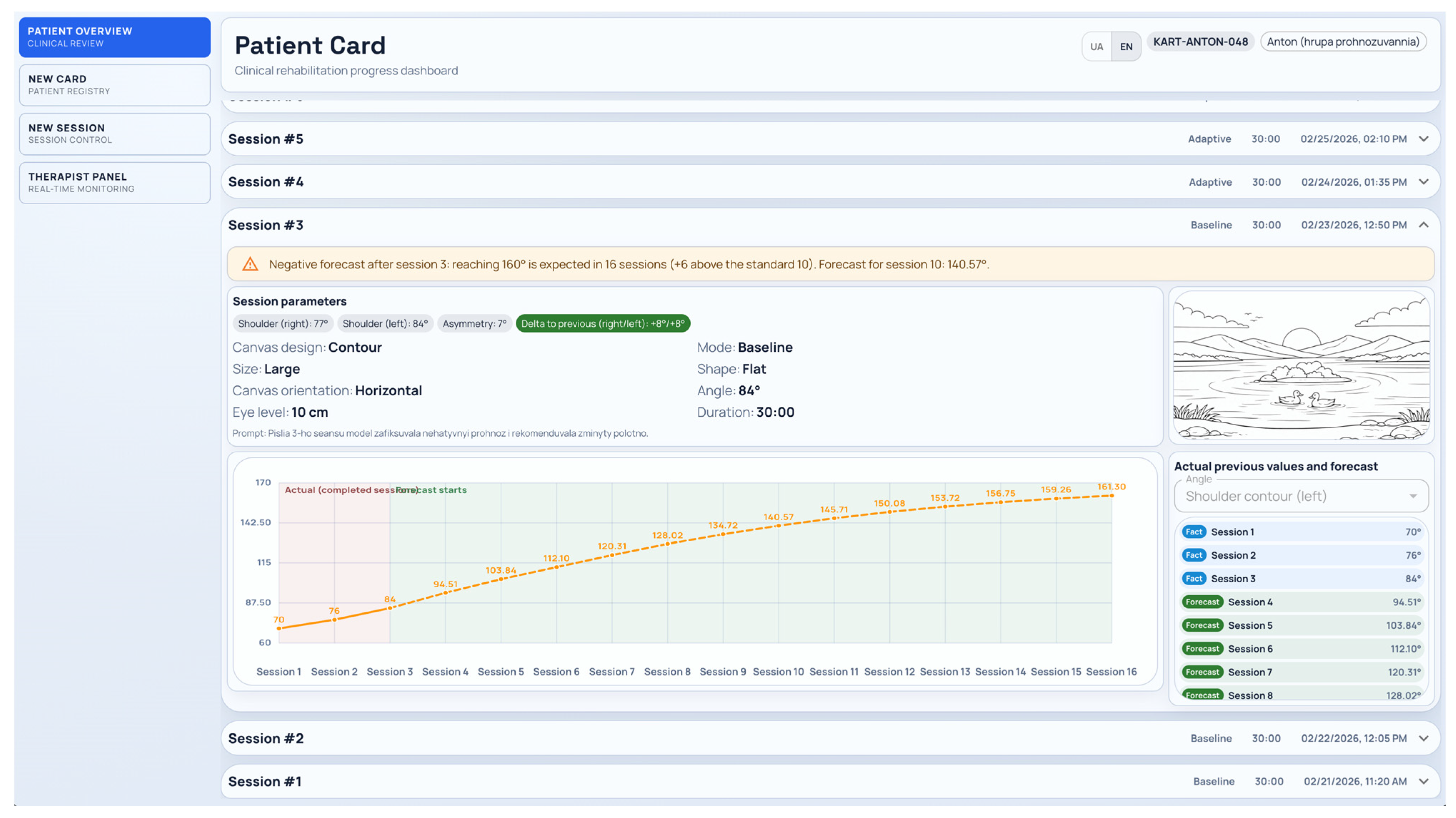
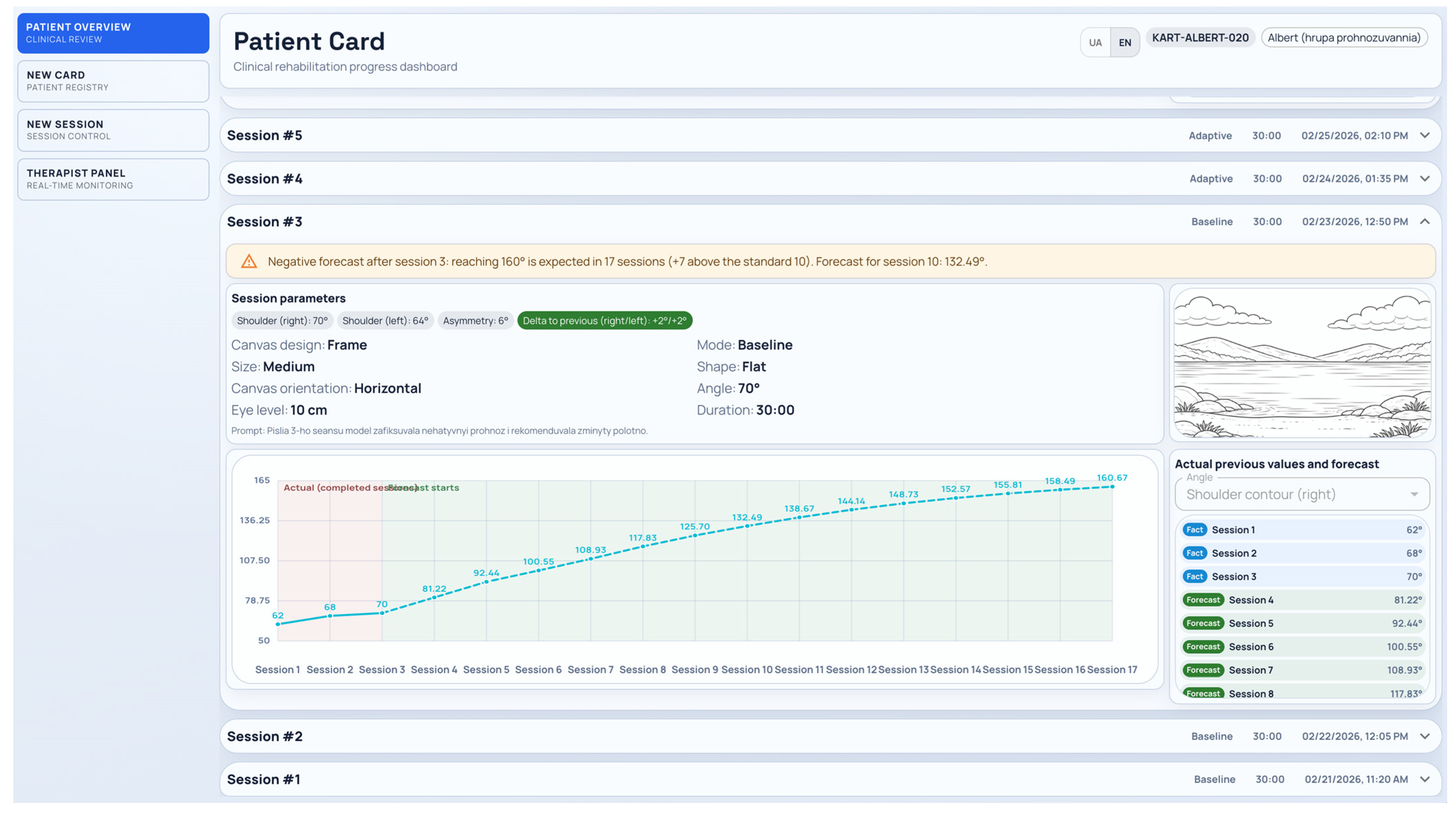
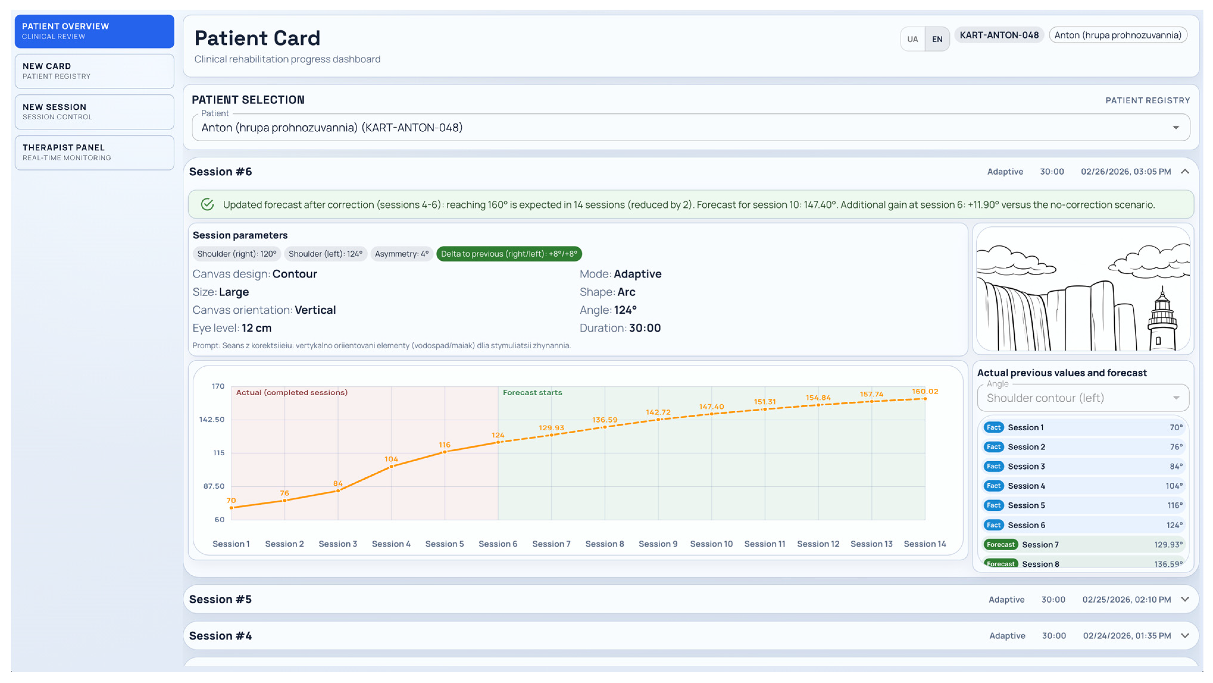
Patient Overview: The main screen displays a kinematic SVG-based progress graph implemented from scratch. It includes six data series (shoulder, elbow, and wrist—left/right) across nine measurement cycles, with color-coded deviations from normative values and predictive intervals visualized as dashed bands. Range-of-motion (ROM) cards present current amplitude values along with directional changes relative to the previous session (↑/↓). The interface also includes a session log and a weekly rehabilitation plan.

Patient Registration (PatientRegistration): The second screen provides the structured input of patient data, including demographic information, diagnosis according to ICD-11, the affected side, and treatment start date. These data establish the context for generating therapeutic images and defining baseline normative thresholds.

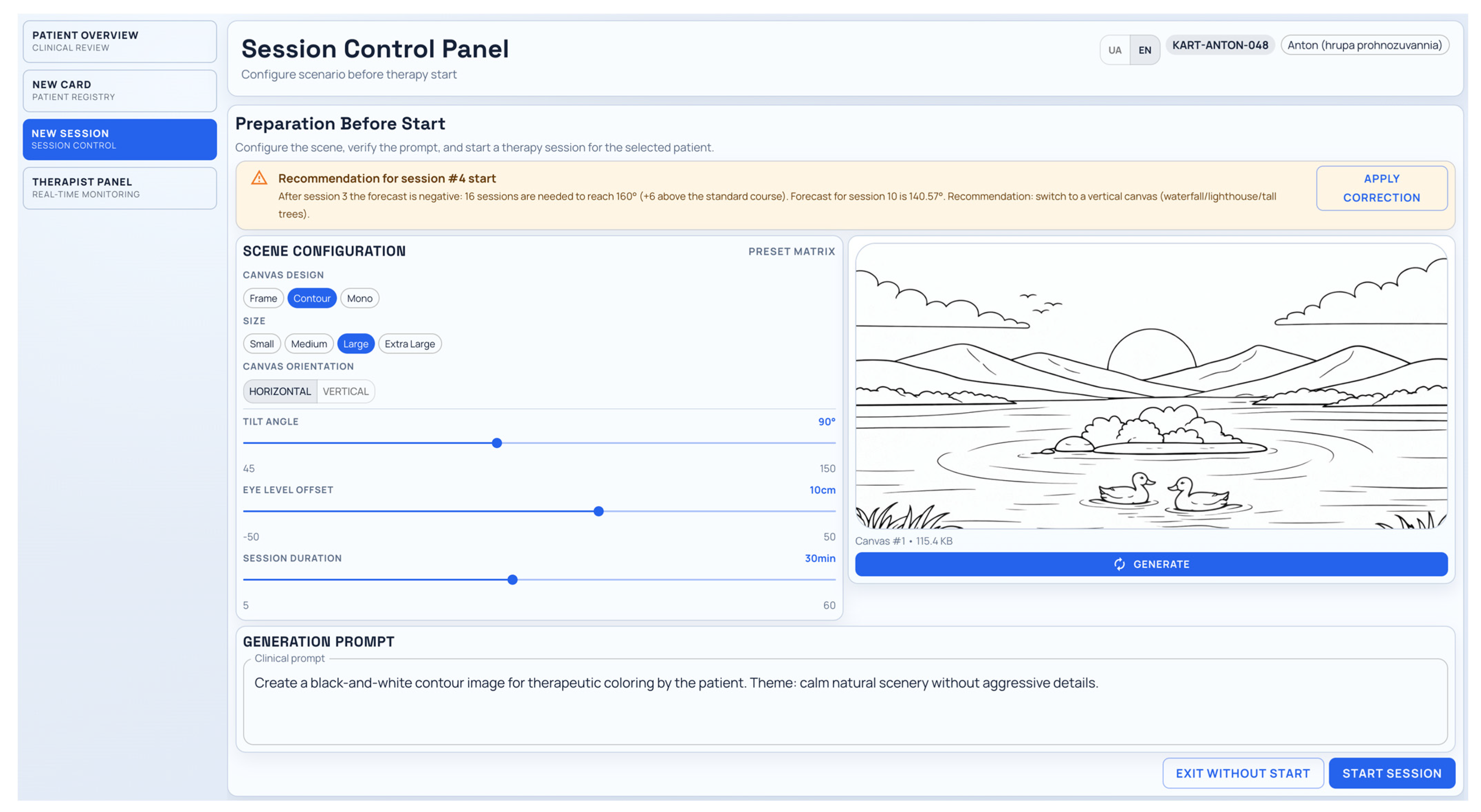
AR Scene Configuration (SessionConsole): The physiotherapist configures AR environment parameters in real time, including environment selection (three options), canvas design, tilt angle (45–150°, step 15°), and vertical offset relative to eye level (−50 to +50 cm). These parameters are encoded into a buildContext string used for the AI-based generation of therapeutic image masks, which are subsequently rendered onto the AR canvas. The interfaces of the web application are illustrated in Figure 5 and Figure 6: the session preparation and configuration panel (Figure 5) and the patient overview with the kinematic progress graph (Figure 6).

5.5. Data Flows Between System Components

The interaction between the four subsystems is organized through four independent data channels (

Table 3. Summary characteristics of the subsystems.

Subsystem	Technology	Interface	Role in Session	Data Outputs
Python video analysis	MediaPipe + Kalman + PyQt5	RTSP/TCP (input), REST (output)	Markerless goniometry	JSON angles (22 parameters)
Unity/Magic Leap 2	Unity 2022 LTS + OpenXR	WebRTC, REST	AR-based art therapy	H.264 video stream
NestJS backend	NestJS + TypeScript	REST API, WebSocket	Signaling, routing	roomId, sessions
React web interface	React 19 + Vite 7	REST, WebRTC	Monitoring, control	Session configuration

). Goniometric Data Channel: Python-based subsystem → NestJS API (POST/api/v1/angles, JSON, ~30 Hz) → React web interface. Each data packet includes a timestamp, session identifier, and an array of 22 joint angle values with associated confidence levels. To minimize latency, the Python subsystem utilizes the non-blocking HTTP client aiohttp.

AR Session Control Channel: React web interface → NestJS API (REST: POST/rooms, PATCH/rooms/:id) → Magic Leap 2 (WebSocket push). Upon any modification of the scene parameters, the NestJS server immediately sends a push notification to the connected headset via Socket.IO without requiring a restart of the AR application. This represents a key clinical feature enabling adaptive session control.

Video Streaming Channel (WebRTC): Magic Leap 2 → WebRTC P2P → physiotherapist’s browser. The NestJS server solely serves as a signaling server; once the peer-to-peer connection is established, media traffic bypasses the server. The end-to-end latency within a local network is approximately 60 ms.

Data Storage Channel for Prediction: The Python subsystem records the complete time series of joint angle measurements into local JSON files using the SessionAngleLogger (~9000 records per 5 min session, with a guaranteed flush after each entry). Additionally, service metadata are stored, including the software version, camera serial numbers, Kalman filter parameters, and per-frame detection quality. This ensures the reproducibility of measurement conditions across sessions, which is essential for accurate comparison of interval model identification results.

6. Method for Identification of Interval Models

Let us consider the formulation for the problem of identifying interval mathematical models describing the recovery dynamics of upper-limb joint mobility angles.

The mathematical model of the recovery dynamics of upper-limb joint mobility angles is considered as a discrete time (difference) equation of the following form [15,50]:

$$v_{i,k}\left(\overrightarrow{V}\right) = f_1\left(\overrightarrow{V}\right)\ast g_1+f_2\left(\overrightarrow{V}\right)\ast g_2+ f_m\left(\overrightarrow{V}\right)\ast g_m, =1,\dots ,I, k=d,\dots ,K,$$

(5)

where $v_{i,k}$ denotes the modeled value of the angle of the $i$-th joint; $\mathbf{g}$ is the vector of model parameters to be estimated based on interval data; $f_1\left(\mathrm{V}\right),f_2\left(\mathrm{V}\right),\dots ,f_m\left(\mathrm{V}\right)$ represent the set of basis functions; $k$ is the discrete time index; and $d$ is the order of the difference equation.

Since Equation (5) is a recursive difference equation, for each basis function, the following vector representation is obtained:

$$\overrightarrow{V}= {(v_{i,k-d},v_{i,k-d+1}, \dots ,v_{i,k})}^T$$

(6)

Assume that estimates $\widehat{\mathrm{g}}$ of the parameter vector $\mathrm{g}$ have been obtained. If the initial conditions for the difference scheme (5) are specified in the form of intervals $\left[{\widehat{v}}_{i,k}\right]$, $i=1,\dots ,I$, $k=1,\dots ,d-1$, then the mathematical model of the recovery dynamics of upper-limb joint mobility angles can be represented as an interval difference equation:

$$\left[v_{i,k}\left(\widehat{\mathrm{V}}\right)\right]=\left[f_1\left(\widehat{\mathrm{V}}\right)\right]{\widehat{g}}_1+\left[f_2\left(\widehat{\mathrm{V}}\right)\right]{\widehat{g}}_2+\cdots +\left[f_m\left(\widehat{\mathrm{V}}\right)\right]{\widehat{g}}_m, i=1,\dots ,I, k=d,\dots ,K.$$

(7)

where $\widehat{\mathrm{V}}=[{\widehat{v}}_{i,k-d},\dots ,{\widehat{v}}_{i,k}]$ is an interval vector whose components are interval estimates $\left[{\widehat{v}}_{i,k}^{-},{\widehat{v}}_{i,k}^{+}\right]$ of joint mobility angles.

In the following, without loss of generality, the index $i$ (denoting the joint angle number) is omitted, since a separate interval discrete dynamic model is constructed for each joint angle.

Based on the hypothesis that the computed interval estimates $\left[{\widehat{v}}_k^{-},{\widehat{v}}_k^{+}\right]$ of the modeled variable must belong to the experimentally obtained numerical intervals $\left[z_k^{-},z_k^{+}\right]$ of the same characteristic for each rehabilitation session $k=1,\dots ,K$, we obtain the following mathematical problem for estimating $\widehat{\mathrm{g}}$ [15,16]:

$$\left\{\begin{array}{l}\left[{\widehat{v}}_0^{-},{\widehat{v}}_0^{+}\right]\subseteq \left[z_0^{-},z_0^{+}\right],\\ ⋮\\ \left[{\widehat{v}}_{d-1}^{-},{\widehat{v}}_{d-1}^{+}\right]\subseteq \left[z_{d-1}^{-},z_{d-1}^{+}\right],\\ z_k^{-}\le \left[f_1\left({\widehat{\mathrm{V}}}_r\right)\right]{\widehat{g}}_1+\left[f_2\left({\widehat{\mathrm{V}}}_r\right)\right]{\widehat{g}}_2+\cdots +\left[f_m\left({\widehat{\mathrm{V}}}_r\right)\right]{\widehat{g}}_m\le z_k^{+},\\ k=d,\dots ,K.\end{array}\right.$$

(8)

The resulting system represents an interval system of nonlinear algebraic equations (ISNAE) with respect to the unknown components of the parameter vector $\mathrm{g}$. The Expressions $\left[{\widehat{v}}_0^{-},{\widehat{v}}_0^{+}\right]\subseteq \left[z_0^{-},z_0^{+}\right],\dots ,\left[{\widehat{v}}_{d-1}^{-},{\widehat{v}}_{d-1}^{+}\right]\subseteq \left[z_{d-1}^{-},z_{d-1}^{+}\right]$ serve as the initial conditions for the difference scheme (7).

Expression (7) is referred to as an interval discrete model of the recovery dynamics of upper-limb joint mobility angles. In general, both the structure and the parameters of this model are unknown. Therefore, two problems must be addressed: structural identification and parametric identification of the interval discrete model.

Let us consider the problem of the structural identification of interval models describing the recovery dynamics of upper-limb joint mobility angles. In contrast to the parametric identification problem, the vector of basis functions in the structural identification problem is unknown.

To represent the mathematical model of the dynamics, we introduce the concept of a set of structural elements:

$${\lambda }_s=\left\{f_1^s\left(v_{k-d},\dots ,v_{k-1}\right)\ast g_1^s,\dots ,f_m^s\left(v_{k-d},\dots ,v_{k-1}\right)\ast g_m^s\right\}$$

(9)

In Expression (9), $s$ denotes a specific set of structural elements used to construct the $s$-th model; ${\lambda }_s$ is used to denote the corresponding structure.

The mathematical models considered in the structural identification process take the following form:

$$v_k\left({\lambda }_s\right)=f_1^s(v_{k-d},\dots ,v_{k-1})g_1^s+\cdots +f_m^s(v_{k-d},\dots ,v_{k-1})g_m^s.$$

(10)

Given the experimentally obtained interval data, the consistency condition of the model with the data is formulated as:

$$v_k({\lambda }_s,{\mathrm{V}}_k)\in [z_k^{-},z_k^{+}], \forall k=0,\dots ,K,$$

(11)

where $z_k^{-},z_k^{+}$ are the lower and upper bounds of the experimentally observed values, and $v_k({\lambda }_s,{\mathrm{V}}_k)$ is the true value of the modeled characteristic for a fixed structure ${\lambda }_s$ and fixed input vector ${\mathrm{V}}_k=(v_{k-d},\dots ,v_{k-1}{)}^T$.

Taking condition (11) into account, we obtain the following system:

$$\left\{\begin{array}{c}{z}_0^{-}\le f_1^s\left({\overrightarrow{V}}_0\right)\ast g_1^s+\cdots +f_m^s\left({\overrightarrow{V}}_0\right)\ast g_m^s\le z_0^{+}\\ ⋮\\ z_{d-1}^{-}\le f_1^s\left({\overrightarrow{V}}_{d-1}\right)\ast g_1^s+\cdots +f_m^s\left({\overrightarrow{V}}_{d-1}\right)\ast g_m^s\le z_{d-1}^{+}\\ z_d^{-}\le f_1^s\left({\overrightarrow{V}}_d\right)\ast g_1^s+\cdots +f_m^s\left({\overrightarrow{V}}_d\right)\ast g_m^s\le z_d^{+}\\ ⋮\\ z_K^{-}\le f_1^s\left({\overrightarrow{V}}_K\right)\ast g_1^s+\cdots +f_m^s\left({\overrightarrow{V}}_K\right)\ast g_m^s\le z_K^{+}\end{array} \right.$$

(12)

Since the first $d$ interval equations correspond to initial conditions, the system can be rewritten as:

$$\left\{\begin{array}{l}[{\widehat{v}}_0^{-},{\widehat{v}}_0^{+}]\subseteq [z_0^{-},z_0^{+}],\dots ,[{\widehat{v}}_{d-1}^{-},{\widehat{v}}_{d-1}^{+}]\subseteq [z_{d-1}^{-},z_{d-1}^{+}],\\ z_k^{-}\le f_1^s\left({\mathrm{V}}_k\right)g_1^s+\cdots +f_m^s\left({\mathrm{V}}_k\right)g_m^s\le z_k^{+}, k=d,\dots ,K.\end{array}\right.$$

(13)

After performing the above transformations, the general form of the parametric identification problem for interval models of the recovery dynamics of upper-limb joint mobility angles is obtained in the form of an interval system of nonlinear algebraic equations (ISNAE) for a given candidate model s. It is well known that the ISNAE (15,16) admits multiple solutions if it is consistent [15,50]. However, for constructing a mathematical model of the dynamics, it is sufficient to obtain at least one feasible solution for this system:

$$\begin{gathered} \delta \left({\lambda }_s\right)\stackrel{{\lambda }_s=\left\{f_1^s\left(\overrightarrow{V}\right)\ast g_{l1}^s,\dots ,f_{m_s}^s\left(\overrightarrow{V}\right)\ast g_{l{m}_s}^s\right\}}{\to }min, \\ {m}_s\in \left[I_{min},I_{max}\right],f_1^s\left(\overrightarrow{V}\right),f_{m_s}^s\left(\overrightarrow{V}\right)\in F,{\widehat{g}}_{jl}^S\in \left[g_{jl}^{-};g_{jl}^{+}\right],j=1,\dots ,m, l=1,\dots ,S \end{gathered}$$

(14)

where $m_s$ denotes the number of structural elements in the $s$-th interval model, $[I_{\mathrm{m}\mathrm{i}\mathrm{n}},I_{\mathrm{m}\mathrm{a}\mathrm{x}}]$ is the minimum and maximum number of structural elements in the model, $S$ is the number of candidate models, F is the set of potential structural elements, and ${\widehat{g}}_{jl}^s$ is the vector of parameter estimates of the candidate model with structure ${\lambda }_s$.

The procedure for evaluating solutions of the ISNAE for a fixed candidate model $s$ is based on assessing the quality of parameter estimates of the mathematical model. Instead of directly using the objective function $\delta \left({\lambda }_s\right)$, the quality of parameter estimation is evaluated using the function $\delta \left({\widehat{\mathrm{g}}}_l\right)$.

This function represents the difference between the midpoints of the most distant predicted and experimental intervals for each time step if these intervals do not intersect. If the intervals intersect, $\delta \left({\widehat{\mathrm{g}}}_l\right)$ is defined as the minimal width of their intersection. The function $\delta \left({\widehat{\mathrm{g}}}_l\right)$ is defined as follows [15,50]:

$$\begin{gathered} \delta \left({\widehat{\overrightarrow{g}}}_l\right)= \underset{i=1,\dots ,N}{\max }\left\{\left|\left.\left.mid\left(\right[{\widehat{v}}_k\left]\right)-mid({[z}_k^{-};z_k^{+}])\right|\right\},\right.\right. \\ if {\left[{\widehat{v}}_k\right]\cap [z}_k^{-};z_k^{+}]=\varnothing ,\exists k=0,\dots ,K \end{gathered}$$

(15)

$$\begin{gathered} \delta \left({\widehat{\overrightarrow{g}}}_l\right)=\underset{i=1,\dots ,N}{\max }\left\{w\left.id\left(\right[{\widehat{v}}_k\left]\right)-wid({\left[{\widehat{v}}_k\right]\cap [z}_k^{-};z_k^{+}])\right\}\right., \\ if {\left[{\widehat{v}}_k\right]\cap [z}_k^{-};z_k^{+}]=\varnothing , \forall k=0,\dots ,K \end{gathered}$$

(16)

As can be observed, the objective function is sufficiently complex, nonlinear, and defined algorithmically. In this case, solving the optimization problem (14) requires the use of metaheuristic algorithms, in particular, the method based on the behavioral model of a bee colony [16]. Let us consider the main phases of this method [51].

The core idea of the method is based on an analogy between searching for optimal model parameters and the process by which a bee colony searches for nectar sources with the highest yield. Within the context of bee colony behavior, nectar collection is divided into several phases [52,53]: the scout bee phase, the employed bee phase, and the onlooker bee phase.

Scout bees explore the search space randomly during the initial phase and evaluate potential nectar sources. The quality of a nectar source is represented by a quantitative measure that depends on the amount of nectar and the distance from the hive. After returning to the hive, scout bees share information with employed bees. The latter then selects which nectar source to exploit, with higher-quality sources attracting a larger number of bees. Once a source is depleted, the process returns to the scout bee phase.

The algorithm is based on the behavioral phases of a bee colony. The first step involves defining the initial variables: interval data obtained during the experiment and parameters of the structural identification algorithm, including SSS—the number of candidate models; MCN—the total number of iterations; LIMIT—a parameter defining source exhaustion; $\left[I_{min},I_{max}\right]$—the minimum and maximum number of structural elements in the model; and $F$—the set of potential structural elements. In addition, the stopping criteria, execution strategy (sequential or parallel), and the lower and upper bounds of the parameter estimates of the candidate model are specified.

During the initialization phase, the initial set of candidate models ${\mathsf{\Lambda }}_0$ of size S is generated randomly from the set of structural elements $F$. For each model, the value of the objective function is computed using the parametric identification algorithm.

The employed bee phase is responsible for generating the set of current models ${\mathsf{\Lambda }}_{mcn}^{\prime }$. Based on a model ${\lambda }_s$, a new model ${\lambda }_s^{\prime }$ is constructed as its neighborhood. This new model is formed by randomly selecting and replacing a subset of structural elements of the current model ${\lambda }_s$. The number of elements to be replaced, denoted as $n_s$, depends on the quality $\delta \left({\lambda }_s\right)$ of the current model, which is evaluated using the function $\delta \left({\widehat{\overrightarrow{g}}}_l\right)$, according to Expressions (14) or (15), for a fixed model structure and number of elements $m_s\in \left[I_{min},I_{max}\right]$. At this stage, a selection procedure is performed to choose the better model between the current and the generated one.

In the context of the structural identification problem, the onlooker bee phase corresponds to determining the neighborhood for further exploration of the current model ${\lambda }_s$. The neighborhood is generated using the method described above. The number of models in the neighborhood is determined using a probabilistic approach described by Equation (17):

$$P_s\left({\lambda }_s^1\right)={\displaystyle \frac{1-\delta \left({\lambda }_s^1\right) }{{\displaystyle {\sum }_{s=1}^S}\left(1-\delta \left({\lambda }_s^1\right) \right)}}, s=1\dots S$$

(17)

The exact number of newly generated models in the neighborhood is determined as $m_s={int(P}_s\ast S)$. For each model, a counter variable limit is introduced, representing the exhaustion of a nectar source in the context of the bee colony behavioral model and serving as a mechanism for escaping local minima in the structural identification optimization problem.

At this stage, group selection is performed for each generated neighborhood of the current model ${\lambda }_s$. The value of the limit counter is incremented by one each time the current model is not updated during the group selection process.

In the next step, the model with the minimum value of the objective function $\delta \left({\lambda }_s\right)$ is selected. If $\delta \left({\lambda }_s\right)$ = 0, the structural identification procedure is terminated; otherwise, the algorithm proceeds to the next phase.

The scout bee phase implements a mechanism for escaping local minima. If the limit counter of the current model ${\lambda }_s$ exceeds the predefined threshold LIMIT, specified during initialization, the model is considered trapped in a local minimum and must be replaced. A new model is then generated randomly, similarly to the initialization phase.

As previously noted, whenever the set of structural elements is modified for each candidate model, the optimal parameter estimates are determined using the same metaheuristic algorithm. Let us now consider the details of this procedure.

Before the algorithm starts, the input data and parameters are defined: interval data (5); model structure (7); $S$—the total population size (number of bees); $MCN$—the total number of iterations; mcn = 1—the current iteration index; and LIMIT—a parameter defining the exhaustion threshold of a nectar source.

Initialization phase (scout bees): At this stage, the parameter vectors ${\widehat{\overrightarrow{g}}}_l$ are initialized randomly using the following rule:

$$\left[{\widehat{g}}_{jl}^{-};{\widehat{g}}_{jl}^{+}\right]={[g}_{jl}^{low}]+rand\left(0,1\right)\ast \left(g_{jl}^{up}-g_{jl}^{low}\right), j=1,\dots ,m, l=1,\dots , S.$$

(18)

Next, the values of the objective function are computed according to Expressions (14) or (15). As can be observed, the evaluation of the objective function is independent for each parameter vector ${\widehat{\overrightarrow{g}}}_l$ generated using Expression (18). Therefore, these computations can be efficiently performed in parallel.

If the number of computational nodes is $N$, the entire set of parameter vectors ${\widehat{\overrightarrow{g}}}_l$ $l=1,\dots , S$ is partitioned into $N$ subsets, each processed independently.

Employed bee phase: In the context of the optimization problem, this phase corresponds to searching for new parameter estimates that lead to a reduction in the objective function value. Such estimates of the parameter vector are computed as follows:

$${\widehat{g}}_{jl}^{mcn}={\widehat{g}}_{jl}+{\mathsf{\Phi }}_{jl}\ast \left({\widehat{g}}_{jl}-{\widehat{g}}_{jp}\right), j=1,\dots ,m,p \ne l=1,\dots , S,$$

(19)

where ${\mathsf{\Phi }}_{jl}$ is a random number drawn from the [−1;1], $j=1,\dots ,m$ denotes a randomly selected parameter index; and $\widehat{g}$ is a randomly selected parameter vector (nectar source) such that $p \ne l=1,\dots , S$.

If the obtained parameter value does not satisfy the constraint ${\widehat{\overrightarrow{g}}}_l\in \left[g_{jl}^{low};g_{jl}^{up}\right]$, then instead of Expression (19), the following update rule is applied:

$${\widehat{g}}_{jl}^{mcn}={\widehat{g}}_{jl}-{\mathsf{\Phi }}_{jl}\ast \left({\widehat{g}}_{jl}-{\widehat{g}}_{jp}\right), j=1,\dots ,m,p \ne l=1,\dots , S$$

(20)

Next, a pairwise comparison of the objective function values is performed between the current and the newly computed parameter estimates:

$${\widehat{\overrightarrow{g}}}_l=\left\{{\widehat{\overrightarrow{g}}}_l, if \delta \left({\widehat{\overrightarrow{g}}}_l\right) \le \delta \left({\widehat{\overrightarrow{g}}}_l^{mcn}\right)\right\}\mathrm{or} {\widehat{\overrightarrow{g}}}_l=\left\{{\widehat{\overrightarrow{g}}}_l^{mcn}, if \delta \left({\widehat{\overrightarrow{g}}}_l\right) > \delta \left({\widehat{\overrightarrow{g}}}_l^{mcn}\right)\right\}$$

(21)

After that, the trial counter (representing the exhaustion level of the nectar source) $limit < LIMIT$ is incremented for the obtained parameter vector $\widehat{\overrightarrow{g}}$, enabling the algorithm to escape local minima in subsequent iterations.

As can be observed, the evaluation of the objective function remains independent for each parameter vector ${\widehat{\overrightarrow{g}}}_l$ generated using Expressions (19) and (20). Therefore, these computations can also be efficiently performed in parallel.

Onlooker bee phase: In the context of the optimization problem, this stage is responsible for identifying the most promising points (parameter vectors) in whose neighborhood a more detailed exploration of the objective function should be performed. For this purpose, for each point obtained in the previous phase, the probability $P_l$ is computed as follows:

$$P_l={\displaystyle \frac{1-\delta \left({\widehat{\overrightarrow{g}}}_l\right) }{{\displaystyle {\sum }_{l=1}^S}(1-\delta \left({\widehat{\overrightarrow{g}}}_l\right))}}$$

(22)

It should be noted that the values of $\left({\widehat{\overrightarrow{g}}}_l\right)$ are preliminarily normalized to 1. Based on the probabilities computed using Expression (22), the number of points for exploring the neighborhood of potential local minima of the objective function is determined as $m_l={int(P}_l\ast S)$. Accordingly, if $m_l>0$, then $m_l$ neighboring points are generated using Expressions (19) or (20). After computing the coordinates of each point in the neighborhood, $N$ computational threads are organized, similarly to the previous phases. Within each thread, for points where $m_l>0$, the objective function values are evaluated and compared pairwise with the current parameter estimates according to Expression (21).

The next step is to identify the point with the minimum value of the objective function at the current iteration. If $\delta \left({\widehat{\overrightarrow{g}}}_l\right)=0$, the optimization procedure is terminated. Otherwise, the counter is reset by setting $limit=0$, and the algorithm returns to the beginning of this phase.

Scout bee phase: This phase is used to avoid stagnation in local minima of the objective function. In terms of the bee colony behavioral model, this phase is activated when a nectar source becomes exhausted. For each point, it is checked whether its trial counter limit exceeds the predefined threshold $LIMIT$. If this condition is satisfied, the corresponding parameter vector is replaced by a new estimate generated using Expression (18). After that, the algorithm returns to the employed bee phase.

To ensure convergence of the iterative procedure when solving problem (14), it is necessary to guarantee a sequence of objective function values $\delta \left({\widehat{\overrightarrow{g}}}_1\right),\dots ,\delta \left({\widehat{\overrightarrow{g}}}_l\right)$that satisfies the following condition [16]:

$$\delta \left({\widehat{\overrightarrow{g}}}_1\right)> \delta \left({\widehat{\overrightarrow{g}}}_2\right)>,\dots ,\delta \left({\widehat{\overrightarrow{g}}}_{l=L }\subset \Omega \right),$$

(23)

where $\mathsf{\Omega }$ denotes the solution space of the ISNAE.

7. Results and Discussion

7.1. Overall Organization of the Clinical Study

To validate the developed software modules and to evaluate the proposed interval mathematical models of joint mobility recovery dynamics, a clinical study was conducted at the immersive hub of the West Ukrainian National University. The study was designed as a two-stage sequential experiment that reflects a realistic clinical deployment scenario of the system: first, data acquisition and construction of a predictive model, followed by the application of this model for real-time support of new patients with adaptive adjustment of the therapeutic protocol.

Five patients with different orthopedic diagnoses participated in the study and were divided into two groups according to the experimental stage. The training group (three patients) completed a full course of 10 AR-based rehabilitation sessions, during which only kinematic data were collected without predictive modeling. The prediction group (two patients) underwent rehabilitation with active use of the interval mathematical model constructed based on the training group data, enabling the real-time prediction of recovery trajectories and generation of recommendations for adaptive adjustment of the therapeutic protocol.

As the primary indicator for constructing and validating the interval mathematical model, the shoulder joint flexion angle was selected, with a normative range of 160–180° (according to AAOS standards [43]). This choice is justified by several factors. First, shoulder flexion is one of the most functionally significant movements of the upper limb, directly involved in daily activities such as reaching, dressing, and personal hygiene, and serves as a key indicator of functional recovery. Second, during AR-based art therapy tasks performed on a vertical canvas, shoulder flexion is the dominant movement, establishing a direct relationship between therapeutic activity and the measured parameter. Third, this movement can reliably be captured by the three-camera video analysis system: the frontal camera (FRONT) provides an optimal viewpoint for measuring flexion, with the projection error not exceeding 3–5° [39,54,55]. Fourth, impaired shoulder flexion is a common clinical feature across all five patient diagnoses, allowing the use of a unified model for the comparative analysis of recovery dynamics.

7.2. Model Construction Stage: Training Group

The training group consisted of three patients with different degrees of shoulder joint mobility limitation:

Anastasiia (25 years old, female)—subacromial bursitis of the right upper limb. The initial shoulder flexion angle was 140°, corresponding to a moderate limitation (a deficit of 20–40° from the lower bound of the normative range). Bursitis is characterized by pain during active movement in extreme positions, resulting in cautious motor behavior and a gradual recovery trajectory.

Valentyna (22 years old, female)—epicondylitis of the right elbow joint. The initial shoulder flexion angle was 130°. Although the primary diagnosis concerns the elbow joint, the inflammatory process and pain syndrome limit the overall motor activity of the upper limb, including the compensatory restriction of shoulder joint motion. The patient’s young age and absence of structural damage to the joint capsule suggest a potentially high recovery rate.

Serhii (42 years old, male)—post-traumatic adhesive capsulitis of the right shoulder joint (“frozen shoulder”). The initial flexion angle was 60°, corresponding to a severe limitation (a deficit of 100–120°). Adhesive capsulitis represents the most challenging diagnosis among those considered, as it involves fibrotic changes in the joint capsule and is characterized by a prolonged recovery period with nonlinear dynamics (slow initial phase followed by gradual acceleration).

Each patient in the training group completed 10 AR-based rehabilitation sessions, each lasting 5 min, with a frequency of 2–3 sessions per week. During each session, the patient wore a Magic Leap 2 headset and performed an art-therapy task—coloring a therapeutic image on a virtual canvas using hand gestures in AR space. The initial coloring template was selected by the physiotherapist via the SessionConsole, taking into account the diagnosis and baseline mobility level. For the training group, a template with a balanced spatial distribution of elements across the canvas was used, promoting movements in multiple directions.

Simultaneously with the execution of the AR-based art-therapy tasks, the Python-based markerless video analysis subsystem acquired kinematic data in real time using three stationary IP cameras positioned in the FRONT, LEFT, and RIGHT configurations. Human pose estimation was performed using the neural network-based MediaPipe Pose Landmarker framework [41,42], which detects 33 anatomical skeletal landmarks. To improve measurement stability and suppress detection noise, the obtained trajectories were additionally processed using Kalman filtering (Equations (1)–(4)).

The multi_camera.py module dynamically selected the optimal camera view for each joint angle estimation according to landmark visibility confidence scores, while geometric fusion of multiple viewpoints reduced the projection-related measurement errors to approximately 3–5° under controlled rehabilitation room conditions. The SessionAngleLogger module continuously recorded all 22 joint angle parameters in JSON format at a frequency of approximately 30 frames per second, resulting in nearly 9000 records during a single 5 min rehabilitation session. In addition to angular measurements, the system stored auxiliary metadata, including software version information, Kalman filter parameters, and frame-level pose-detection quality indicators, thereby ensuring reproducibility of the measurement conditions and subsequent analyses.

As a result, a complete time series of shoulder flexion angle measurements across 10 rehabilitation sessions was obtained for each patient in the training group. The resulting dataset consisted of 10 aggregated representative values (median values calculated for each session) together with corresponding interval estimates reflecting intra-session variability and measurement uncertainty. These interval datasets were subsequently used as input data for the structural and parametric identification of the proposed mathematical models describing rehabilitation dynamics.

7.3. Structural and Parametric Identification of the Interval Model

Based on the collected time series of joint angle measurements from the three patients in the training group, structural and parametric identification of the interval mathematical model describing the recovery dynamics of the shoulder flexion angle was performed using the artificial bee colony (ABC) algorithm (Section 4). The identification procedure consisted of two sequential stages.

During the structural identification stage, the optimal structure of the difference Equation (7) was determined, including the number of previous time series values (order ddd), the set of basis functions, and the overall form of the model. The artificial bee colony algorithm explored a set of candidate models, minimizing the objective function (16), which quantifies the consistency between predicted and experimentally observed intervals.

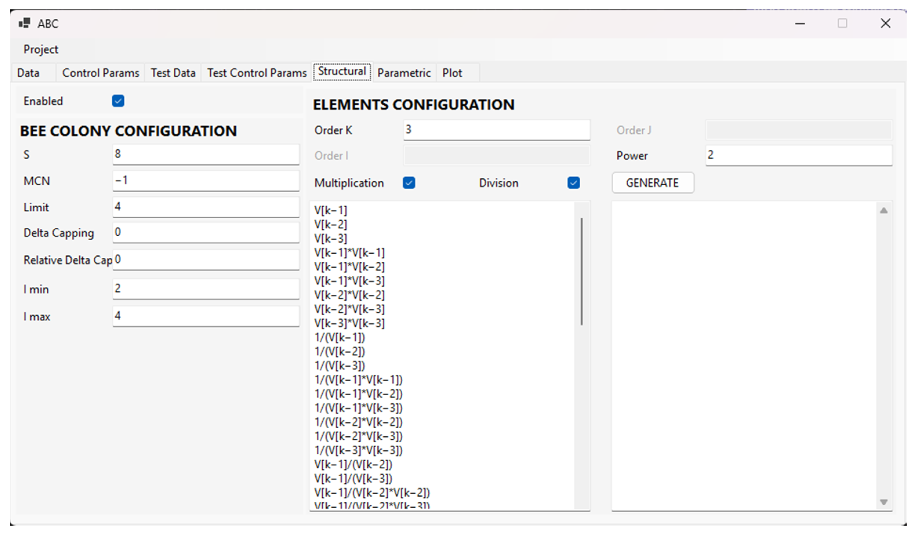
As a result of structural identification, it was established that an adequate model requires $d=3$ previous time series values as initial conditions for the difference scheme. This implies that predicting the joint angle value for the next session only requires the results of the three preceding sessions. The prediction uncertainty was defined as $dZ = 0.1°$, which determines the width of the initial uncertainty intervals. The interface of the developed module for structural identification is shown in Figure 7.

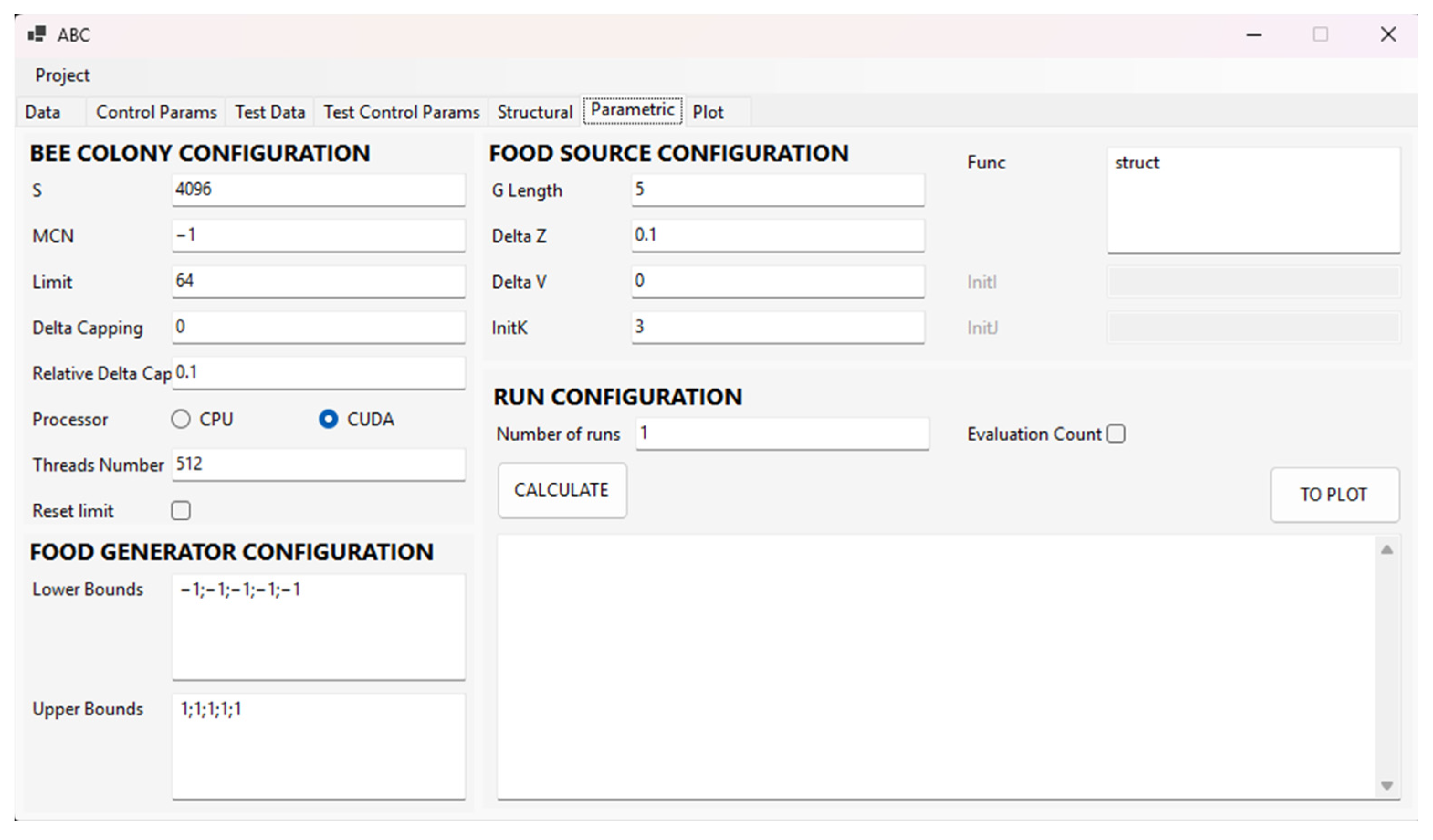
During the parametric identification stage, the parameter vector estimates for the identified optimal model structure were determined to achieve the best agreement between the predicted interval values and the experimental interval data. The artificial bee colony algorithm was used to solve the optimization problem (14) with the objective function (16), which accounts for both the overlap between predicted and experimental intervals and the distance between their midpoints in the case of non-overlapping intervals.

The parametric identification procedure was performed iteratively until the convergence conditions (23) were satisfied. The interface of the developed parametric identification module is presented in Figure 8.

7.4. Mathematical Model of Shoulder Flexion Recovery Dynamics (160–180°)

The identified structure of the interval mathematical model for the recovery dynamics of the shoulder flexion angle (160–180°) of the upper limbs is defined as follows. Initial conditions: three previous time steps ($d=3$), with uncertainty level $dZ=0.1$. The general form of the model is given by:

$$v_{\left[k\right]} = G_{\left[0\right]}+G_{\left[1\right]}\ast v_{[k-1]}+G_{\left[2\right]}\ast v_{[k-3]}+G_{\left[3\right]}\ast v_{[k-1]}\ast v_{[k-2]}$$

(24)

The parameter values obtained from the solution of the parametric identification problem are:

$${G_{\left[0\right]}=0.5566865 G}_{\left[1\right]}=0.97192764 G_{\left[2\right]}=0.35143995 G_{\left[3\right]}=-0.0019254182$$

(25)

Thus, the resulting interval model takes the form:

$$v_{\left[k\right]} =0.5566865+0.97192764\ast v_{\left[k-1\right]}+ 0.35143995\ast v_{\left[k-3\right]}-0.0019254182\ast v_{\left[k-1\right]}\ast v_{\left[k-2\right]}$$

(26)

The obtained interval mathematical model of shoulder flexion recovery dynamics was validated using the data from the training group. For all three patients, the predicted values matched the actual measurements within an error range of 1–3°. For Anastasiia (from 140° to 162° over 10 sessions), the model accurately reproduced a gradual monotonic increase in amplitude with a tendency toward stabilization above 160° after the eighth session.

For Valentyna (from 130° to 178°), the prediction error was minimal during the early sessions and increased up to 4° in later stages due to a nonlinear recovery surge typical of young patients without structural joint damage. For Serhii (from 60° to 146°), the model demonstrated the highest accuracy (error < 2°), correctly capturing the characteristic recovery pattern of adhesive capsulitis, namely, a slow initial phase followed by gradual acceleration. The modeling results for the training group are presented in Appendix A.

7.5. Prediction Stage: Validation of the Adaptive Cycle

In the second stage of the study, two patients underwent AR-based rehabilitation with active utilization of the constructed interval mathematical model to predict the recovery dynamics of the shoulder flexion angle and to generate clinical recommendations in real time. In contrast to the training group, where the model was built retrospectively using previously collected data, the system for these patients operated in a prospective mode: After each session, predictive interval values for subsequent sessions were automatically computed, the estimated number of sessions required to reach the normative range (160–180°) was evaluated, and, when necessary, recommendations for adjusting the therapeutic protocol were generated.

Clinical characteristics of the prediction group: Anton (48 years old, male)—osteoarthritis of the right shoulder joint. The initial flexion angle after the first session was 70°, corresponding to severe mobility limitation (a deficit of 90–110° from the normative range). Osteoarthritis is characterized by degenerative changes in articular cartilage, narrowing of the joint space, and reduced mobility due to pain. In the 45–50 age group, the regenerative potential of joint tissues is reduced, resulting in slower recovery dynamics and the need for a prolonged rehabilitation course.

Albert (20 years old, male)—fracture of the right clavicle and humerus. The initial flexion angle was 62°, the lowest among all five patients in the study, corresponding to extremely severe limitation (a deficit of 98–118°). Fracture with prolonged immobilization leads to pronounced atrophy of the rotator cuff muscles and joint stiffness due to capsular contracture. At the same time, the patient’s young age and absence of degenerative joint changes provide a high recovery potential under appropriate and targeted therapeutic loading.

Both patients began AR-based rehabilitation following a standard protocol: 5 min art-therapy sessions using the Magic Leap 2 headset, involving coloring a therapeutic image on a virtual AR canvas. The initial template was selected similarly to the training group, with a balanced spatial distribution of elements to stimulate multidirectional movements.

Sessions 1–3: Initial dynamics and forecast generation. During the first three sessions, the Python-based markerless video analysis subsystem automatically recorded kinematic data. The measured shoulder flexion angles demonstrated a positive but moderate recovery trend. For Anton, the flexion angle increased steadily, 70° (session 1) → 76° (session 2) → 84° (session 3), corresponding to increments of +6° and +8°, with an average rate of approximately 7° per session. This pattern is typical for patients with osteoarthritis at the early stage of rehabilitation, characterized by stable but moderate improvement without abrupt changes due to pain-limited movement.

For Albert, a non-uniform recovery pattern was observed, 62° (session 1) → 68° (session 2) → 70° (session 3), corresponding to increments of +6° and only +2°, with an average rate of approximately 4° per session. The slowdown between sessions 2 and 3 is characteristic of post-fracture patients, where joint mobilization is limited by protective muscle spasm and capsular stiffness. Notably, Albert’s initial mobility level (62°) was the lowest among all participants, further complicating early-stage recovery.

After the third session, the interval mathematical model had sufficient data to generate a full prediction, as the identified model structure requires d = 3 previous time steps. The system automatically computed predictive trajectories for both patients by extrapolating the current dynamics using the difference Equation (4) with parameters obtained from the training group.

The resulting predictions were clinically unfavorable for both patients. For Anton (current value after session 3: 84°, target: 160°, and remaining deficit: 76°), the model predicted gradual growth with a decelerating rate: 94.5° (session 4) → 103.8° (session 5) → 112.1° (session 6) → 120.3° (session 7) → 128.0° (session 8) → 134.7° (session 9) → 140.6° (session 10) → 145.7° (session 11) → 150.1° (session 12) → 153.7° (session 13) → 156.8° (session 14) → 159.3° (session 15) → 161.3° (session 16). Thus, reaching the lower bound of the normative range (160°) was predicted only at session 16, exceeding the standard 10-session protocol by 60%. A gradual deceleration of the recovery rate was observed, from approximately 10.5° per session at the beginning of the prediction horizon to about 2.0° per session at later stages, reflecting the typical asymptotic behavior associated with osteoarthritis.

For Albert (current value after session 3: 70°, target: 160°, and remaining deficit: 90°), the prediction was even less favorable: 81.2° (session 4) → 92.4° (session 5) → 100.6° (session 6) → 108.9° (session 7) → 117.8° (session 8) → 125.7° (session 9) → 132.5° (session 10) → 138.7° (session 11) → 144.1° (session 12) → 148.7° (session 13) → 152.6° (session 14) → 155.8° (session 15) → 158.5° (session 16) → 160.7° (session 17). The normative range was predicted to be reached only at session 17, exceeding the standard protocol by 70%. The low initial recovery rate (~4° per session) combined with a large remaining deficit (90°) resulted in a pessimistic forecast despite the patient’s young age.

A common characteristic of both predictions is that, under the current therapeutic protocol (balanced coloring template), neither patient would reach the normative range within the standard 10-session course: for Anton, the predicted value after session 10 is 140.6° (deficit 19.4°), and for Albert, 132.5° (deficit 27.5°). This served as a key signal for the system to initiate adaptive correction of the therapeutic protocol.

Generation of recommendations and protocol adaptation: The unfavorable forecast was automatically visualized on the physiotherapist’s web panel (PatientOverview). The kinematic progress graph displayed predictive trajectories as dashed lines with interval bands, clearly indicating that the normative range would not be achieved within the standard course. Additionally, the system presented quantitative indicators: “Predicted number of sessions to reach 160°: 16” for Anton and “17” for Albert, along with deviations from the standard protocol (“+6 sessions” and “+7 sessions”, respectively), as shown in Figure 9.

Based on the analysis of predictive data and the comparison of the actual dynamics of the shoulder flexion angle with other joint angle parameters, the system generated a recommendation for the physiotherapist to modify the therapeutic coloring template on the AR canvas to one that stimulates a greater amplitude of movement specifically in the plane of shoulder flexion.

The rationale for this recommendation was based on the analysis of the biomechanical movement profile. The initial template predominantly contained horizontally oriented elements (landscape components, wide color regions, and horizontal lines), which primarily stimulated abduction and adduction movements in the horizontal plane. However, improving the shoulder flexion angle requires vertical movements involving raising the arm upward—movements that were insufficiently activated by the current template.

The physiotherapist accepted the system’s recommendation and promptly modified the therapeutic image via the SessionConsole module of the web interface. The new template emphasized vertically oriented elements, such as tall trees, architectural structures, and vertical abstract compositions. This design deliberately encouraged patients to perform movements with greater shoulder flexion amplitude, as reaching the upper elements of the image required lifting the arm significantly higher, thereby increasing the flexion angle during each drawing action.

Importantly, this modification represents a non-invasive intervention: the patient continues performing the same basic task (coloring on the AR canvas) without being aware of the change in therapeutic strategy, while the biomechanical profile of movements is substantially altered due to the different spatial distribution of visual elements. This highlights a unique advantage of AR-based art therapy as a therapeutic tool—the ability to subtly and unobtrusively guide motor activity through the adaptive modification of creative content.

Sessions 4–6: Dynamics After Therapeutic Protocol Adjustment: After three sessions (4th–6th) with the updated therapeutic template, a pronounced acceleration in the recovery dynamics of shoulder flexion was observed in both patients. For Anton, the measured flexion angles were 104° (session 4) → 116° (session 5) → 124° (session 6). The increase in session 4 was +20° compared to 84° after session 3, nearly three times higher than the average increase during the initial sessions (~7° per session). Subsequent increases of +12° (session 5) and +8° (session 6) form a decreasing sequence typical of an intensive joint mobilization phase: the largest effect occurs immediately after protocol modification, followed by gradual stabilization at a higher level. The average rate of increase during sessions 4–6 was approximately 13.3° per session, which is 1.9 times higher than during sessions 1–3.

For Albert, the effect of adaptation was even more pronounced: 93° (session 4) → 108° (session 5) → 117° (session 6). The increase in session 4 was +23°, nearly six times higher than the average increase during the first three sessions (~4° per session). This rapid improvement can be explained by two factors: (1) the high latent regenerative potential of a young patient, previously underutilized due to the insufficient activation of flexion movements; and (2) the reduction in protective muscle spasm after adaptation to the AR environment during the first three sessions. Subsequent increases of +15° (session 5) and +9° (session 6) also exceeded the initial rate. The average increase during sessions 4–6 reached approximately 15.7° per session, which is 3.9 times higher than during sessions 1–3.

An important observation is that the actual flexion values after protocol adjustment significantly exceeded the predicted values without intervention. For Anton, at session 6, the actual value (124°) exceeded the predicted value without correction (112.1°) by 11.9°. For Albert, the difference was even greater: 117° versus 100.6°, i.e., +16.4°. This quantitatively confirms the effectiveness of adaptive correction, demonstrating that modifying the therapeutic template significantly accelerates recovery compared to a non-adaptive scenario.

Updated Prediction After Adaptation: Improved Recovery Trajectory: After incorporating data from sessions 4–6 into the time series, the interval model was automatically updated, with parameters recalculated to reflect the accelerated recovery dynamics. The updated predictions demonstrated substantial improvement compared to the initial forecast obtained after session 3. For Anton, the updated trajectory from session 7 was 129.9° → 136.6° → 142.7° → 147.4° → 151.3° → 154.8° → 157.7° → 160.0° (session 14). The predicted number of sessions required to reach 160° decreased from 16 to 14 (−12.5%). The predicted value after the standard 10 sessions increased from 140.6° (without correction) to 147.4° (with correction), i.e., an improvement of 6.8°.

For Albert, the updated trajectory was 122.6° → 130.1° → 137.4° → 142.8° → 147.3° → 151.5° → 155.0° → 157.8° → 160.0° (session 15). The predicted number of sessions decreased from 17 to 15 (−11.8%). The predicted value after the standard 10 sessions increased from 132.5° (without correction) to 142.8° (with correction), i.e., an improvement of 10.3°, reflecting the higher regenerative potential of the younger patient (Figure 10).

Comparative Analysis of “Without Adaptation” and “With Adaptation” Scenarios: The comparison of the two forecasting scenarios enables a quantitative assessment of the effectiveness of the adaptive cycle “measurement—prediction—recommendation—correction”.

Recovery rate of shoulder flexion: The average increase per session rose from approximately 7° to 13.3° for Anton (1.9× increase) and from approximately 4° to 15.7° for Albert (3.9× increase). The more pronounced effect in Albert can be explained by the fact that the initial protocol was less suitable for his condition: the low initial angle (62°) required the targeted stimulation of flexion movements, which was not adequately provided by the balanced template.

Predicted number of sessions: A reduction of two sessions was observed for both patients (from 16 to 14 for Anton and from 17 to 15 for Albert). Although the absolute reduction is identical, it is important to note that the correction was applied after only three sessions (i.e., the model was based on just three data points). Additional corrections at later stages of the rehabilitation course (after sessions 6–7) could potentially lead to further reductions in the total treatment duration.

Difference between actual and predicted values: At session 6, the actual flexion angle exceeded the prediction without adaptation by 11.9° for Anton and 16.4° for Albert. This positive deviation confirms that the modification of the therapeutic template produced an additional gain not captured in the initial forecast trajectory, indicating a genuine therapeutic effect rather than a coincidental acceleration of natural recovery.

Clinical Significance of the Results: The obtained results demonstrate several key aspects of the closed-loop paradigm “execution—measurement—prediction—adaptation” implemented in the proposed system.

First, the proposed interval mathematical model enables the early detection of suboptimal rehabilitation dynamics after only three rehabilitation sessions, which corresponds to the minimum number of observations required for forecasting given the selected model order $d=3$. Such early identification of negative rehabilitation trends allows physiotherapists to proactively modify the therapeutic protocol instead of detecting rehabilitation inefficiency only at the final stages of the treatment course when significant clinical time and rehabilitation resources have already been expended.

Second, the recommendation mechanism based on the adaptive modification of therapeutic visual templates demonstrated its effectiveness as a tool for influencing the biomechanical movement profile. In particular, the transition from a balanced visual template to a vertically oriented therapeutic configuration increased movement amplitude in the flexion plane by approximately 2–4 times in terms of the per-session increment of joint angles. Importantly, patients did not perceive this modification as an increase in physical workload because the rehabilitation process remained integrated into the same creative AR-based activity. This contributes to maintaining patient motivation, engagement, and long-term adherence to the rehabilitation program.

Third, the recalibration of the predictive model after modification of the rehabilitation protocol confirms the adaptive capabilities of the interval-based approach. The mathematical model appropriately responds to changes in therapeutic conditions, updates the rehabilitation trajectory according to newly acquired kinematic data, and generates revised estimates of the required number of rehabilitation sessions. Such functionality enables the iterative refinement of rehabilitation strategies and gradual alignment of the predicted rehabilitation duration with the target therapeutic course defined by physiotherapists.

Overall, these results demonstrate that the integration of interval prediction, adaptive AR-based art therapy, and real-time markerless motion analysis enables the implementation of a closed-loop rehabilitation framework capable of dynamically adjusting rehabilitation scenarios according to the patient’s individual recovery trajectory.

8. Conclusions

In this study, a comprehensive AR-based rehabilitation system for upper-limb recovery was developed by integrating four interconnected subsystems: (i) a Python-based markerless video analysis module that processes data from three stationary IP cameras using MediaPipe Pose Landmarker and Kalman filtering; (ii) an AR art-therapy application implemented for the Magic Leap 2 headset using Unity and OpenXR; (iii) a backend server developed with NestJS/TypeScript; and (iv) a physiotherapist-oriented web application implemented in React.

To predict the recovery dynamics of joint mobility, interval mathematical models based on discrete interval difference equations were constructed. Model identification was performed using the artificial bee colony algorithm and rehabilitation data collected from five patients with different clinical diagnoses. This modeling approach was selected because interval models are suitable for rehabilitation scenarios characterized by limited datasets, measurement uncertainty, and inter-patient variability.

The obtained interval models demonstrated promising predictive performance for shoulder joint angles, including flexion (160–180°), extension (50–60°), and abduction (up to 180°), with an error below 5° under the considered experimental conditions. Structural identification showed that three to four previous time steps are sufficient to construct an adequate predictive model. The integration of interval prediction with real-time system components enables the continuous acquisition of kinematic data during AR-assisted therapy sessions and supports the dynamic adaptation of therapeutic protocols through predictive analytics available in the physiotherapist’s web interface. These features make the proposed system a practical tool for personalized rehabilitation, particularly in the context of the increasing need for upper-limb recovery among veterans and post-stroke patients.

Extending the model to additional joint angles, including the elbow and wrist, using the full 33-point skeletal representation provided by MediaPipe Pose Landmarker opens up prospects for comprehensive monitoring of the entire upper-limb kinematic chain. Such functionality may contribute to more efficient use of rehabilitation resources under conditions of limited access to specialized facilities while supporting objective progress tracking. Furthermore, the system provides a technological basis for the development of gamified AR-based rehabilitation applications, in which predictive visualization of recovery trajectories may improve patient motivation and adherence.

Ethical considerations, including the protection of personal biomechanical data, are addressed through local data storage within the rehabilitation facility network and the use of encryption mechanisms to support compliance with GDPR requirements.

Future work should focus on expanding the patient cohort to validate the proposed models on larger and more heterogeneous datasets and on integrating machine-learning techniques for the automated updating of interval model parameters. Limitations associated with markerless tracking, including sensitivity to lighting conditions, partial occlusions, and rapid movements, require further improvement of calibration and filtering algorithms. Overall, the proposed system contributes to the digital transformation of physical therapy by integrating AR-based art therapy, automated goniometry, and interval prediction into a unified clinical cycle: “execution–measurement–prediction–adaptation”.