An Intelligent Learning-Based Model Predictive Control Framework for High-Speed Train Control Under Moving Block Signaling

Featured Application

This publication’s featured application focuses on the intelligent moving block signaling for high-speed railways. A learning-based model predictive control (LMPC) framework is used to enhance train operation performance and energy efficiency while ensuring strict safety and operational constraints.

Abstract

Despite the widespread adoption of model predictive control (MPC) in railway research, the integration of intelligent learning mechanisms into train control systems operating under moving block signaling remains limited, particularly in approaches that preserve constraint satisfaction and industrial feasibility. To address this gap, this paper presents a novel learning-based model predictive control (LMPC) framework for high-speed train control under the moving block signaling principle. Moving block signaling dynamically enforces safe inter-train separation based on the absolute braking distance, imposing stringent safety, comfort, and performance constraints on train operation. The proposed LMPC exploits the repetitive nature of railway operations by progressively improving its control policy through the incorporation of historical operational data into the terminal set of the optimization problem. This learning capability enables the controller to optimize train behavior on a given line while pursuing different control objectives, namely maximum-speed operation for leading trains and minimum safe inter-train separation for following trains, in full compliance with signaling requirements, speed limits, actuator constraints, and comfort-related jerk bounds. Simulation results on a representative high-speed line show that, compared with a conventional non-learning MPC, the proposed LMPC achieves a measurable reduction in traction-related energy consumption while maintaining comparable speed profiles, travel times, and strict constraint satisfaction. These improvements are achieved through a single software-level modification of the train control algorithm, without requiring additional onboard hardware or infrastructure upgrades, positioning the proposed LMPC as a promising and practically viable solution for energy-efficient deployment in high-speed railway operations.

1. Introduction

Artificial intelligence (AI) is seen as a paramount technological tool that might help in the enhancement and improvement of processes, activities, and operations, including those related to the rail sector [1,2]. In addition, moving block is considered the future of rail signaling and train control systems, thanks to its ability to increase a line’s capacity [3]. Hence, this paper focuses on the design of a moving block-based train controller that is enhanced with an intelligent method to improve its performance.

With this aim, this introduction places the designed controller within the current state of the art in the research of train control methods and intelligent algorithms. Thus, this introduction first reviews moving block, while second it analyzes intelligent algorithms for train control systems. Later, the introduction summarizes the paper’s purpose, importance, and conclusions, concluding with the organization of the remainder of this paper.

Moving block denotes a group of train control systems that are all based on the same signaling principle: the use of an absolute braking distance (ABD) to determine the minimum allowed inter-train distance between trains running on the line [4]. The ABD is a distance measurement given by the space needed by the train to completely stop from the current running speed and whose dependence on braking parameters is exclusively given by the train that is being controlled, as in [5].

Nowadays, moving block is considered the most advanced signaling principle in terms of applied-in-industry systems able to increase capacity performance [4]. Compared with the widespread conventional fixed block, in which the line is divided into segments of a predefined length called ‘blocks’ and the train is allowed to move up to the entry of an occupied block, moving block allows the train to move further ahead and closer to the train running in front of it, always ensuring that the ABD is respected [5]. In other words, moving block allows the train to move as close as possible to the in-front train as allowed by its braking specifications, ensuring a complete halt before the current position of the in-front train’s tail or a track element—for instance, a switch. For this reason, moving block requires the controlled train to have a continuous flow of information regarding the position and speed, not only of the proper controlled train but also of the in-front train. This is accomplished by means of radio-based communications, in-cab signaling, and onboard train positioning [3], which is recalibrated by beacons placed along the infrastructure [6].

As previously stated, moving block has already been successfully applied in industry for metro trains under the IEEE 1474 standard, also commonly known as communications-based train control (CBTC) [7]. For conventional and high-speed trains, specifications and studies have been developed during the last decades, aiming for safe and interoperable systems, but its practical implementation is still limited, and therefore, research related to moving block in conventional and high-speed railways is still intensive [3]. These specifications for conventional and high-speed trains have their main examples in the previously named European rail traffic management system level 3 (ERTMS-L3)—whose moving block implementation in the train control subsystem of ERTMS gives place to the previously named European train control system level 3 (ETCS-L3)—[8], as well as in the Chinese train control system level 4 (CTCS-L4) [9]. Note that previous level 3 in ERTMS was recently merged with the previous fixed block level 2 [10]. Thus, prior ERTMS-L3 is now an advanced function of current ERTMS level 2, which now groups fixed block and moving block [10].

As far as intelligent algorithms are concerned, they are a heterogeneous group of AI-based methods that can be used for both rail scheduling and train control applications [3]. The rail scheduling application has received greater research attention than the train control application [1], whose lack of publicly available datasets for AI model training and testing seems to be its main cause for the lack of research within this field [11].

Regarding intelligent algorithms for scheduling applications, they usually rely on measures based on rerouting [12,13], retiming [14,15], reordering, and speed profile redefinition [16,17,18,19]. However, mixed approaches involving several actions are also possible, such as reordering and retiming [20], rerouting and retiming [21,22], and rerouting, retiming and reordering [23]. With this aim in mind, the literature has used genetic algorithms [21], particle swarm optimization [12], random forests [14], reinforcement learning [20,22], and deep reinforcement learning [13,16,17,18,19,23].

Regarding intelligent algorithms for train control applications and based on references [1,24,25,26], it is distinguished between those applications related to the modelling of dynamics and those applications related to the design of an intelligent controller. Concerning the modeling of dynamics, the literature has focused on the development of simulation environments [27] and of state estimators [28,29] by means of recurrent neural networks [27] and long short-term memory neural networks [28,29]. Concerning the design of intelligent controllers, rail literature has focused on the development of AI-algorithms, usually deep reinforcement learning [30], to substitute conventional controllers [30]. However, there are concerns about the accuracy and constraint satisfaction of these AI-based controllers that substitute conventional controllers, even if they only partially substitute the controller [31]. To overcome this drawback, non-rail literature has recently applied intelligent methods within conventional controllers to enhance them, such as the controller based on a time-delay compensation accompanied by a disturbance rejection neural network as in [32], rather than to completely or partially substitute them. This conventional controller enhancement was proposed to be accomplished by means of learning model predictive control (LMPC) [24,25], which arises as the most promising technique for train control given that model predictive control (MPC) has been a hot topic in recent research, as shown in the literature review in [5].

As a controller designed according to the MPC technique, LMPC is designed as an optimization problem, subject to a set of constraints. As with most of the controllers that are common in control theory, the LMPC’s optimization problem considers a model of system dynamics and its explicitly defined parameters [25]. However, when comparing to conventional MPC, as the cloud-based MPC in [33], LMPC’s differentiating characteristic relies on the introduction of data from previous experiences into the optimization problem so that the controller’s control policy might be enhanced [34,35]. This introduction of data, which reminds one of machine learning techniques, gives LMPC a learning capability from previous executions of the controller [34,35], while respecting the optimization problem’s constraints and taking into account the explicitly modeled system dynamics and parameters [25].

Hence, LMPC provides a hybrid solution that is a middle ground between the machine learning-substituting controller and conventional control theory. This solution enhances the controller’s control policy thanks to the learning capability, while complying with the system’s constraints and stability thanks to the optimization problem’s constraints [25]. This constraint fulfillment makes LMPC a reliable safe controller appropriate for the control of vehicles. Moreover, compared with the AI-substituting alternative, LMPC reduces the amount of data that is necessary for training, since it can be used for a start with low volumes of data and learn and improve in future executions [34,35]. Nevertheless, when also comparing with the AI-substituting alternative, LMPC’s main drawback is considered to be its online execution time when controlling the system, which is related to the computation time that is needed to solve the optimization problem. For this reason, when designing an LMPC, it is important to assess that computation times remain within tolerable limits for an online implementation (see, for instance [26]).

As far as we are concerned in the rail sector, LMPC has only been recently applied for a scheduling application [36], which involved a retiming measure and it was based on a long-short term memory neural network integrated with an MPC. However, LMPC remains unexplored for train control applications; a gap that this paper presumes to cover. The use of LMPC for this application seems appropriate since rails have a repetitive operation on track-guided longitudinal movement and operate under a clear control policy, such as move as fast as possible or as close as possible to other trains. In this paper, note that a high-speed moving block application is covered; a virtual coupling application, which is based on the relative braking distance inter-train distance, was assessed in [26].

This paper does not aim to compare the proposed LMPC with different controller types to identify the best-performing approach. Instead, since the LMPC is obtained by introducing a learning mechanism into a classical non-learning MPC, the comparison is limited to this specific non-learning MPC. Both controllers share the same control policy, constraints, and tuning parameters (

Table 1. High-speed train parameters.

Parameter	Value	Parameter	Value
$M$ (kg)	457,400	$H_p$ (steps)	20
$L^p$ (m)	200	$H_c$ (steps)	1
$A$ (N)	3383.5	$t_s$ (s)	0.2
$B$ (N/(m/s))	114.55	$v_{max}$ (m/s)	97.2
$C$ (N/(m/s)2)	7.32	$v_{min}$ (m/s)	0.5
$\tau$ (s)	0.7	$d_{des}$ (m)	10
$u_{max}$ (N)	224,126	$d_{min}$ (m)	4
$P_{max}$ (W)	8.8 × 106	$b$ (m/s2)	0.5
$\mu$	0.05	$j_{max}$ (m/s3)	0.98
$g$ (m/s2)	9.8	Coaches per trainset	8

), allowing the direct assessment of the impact of the learning mechanism while avoiding biases arising from fundamentally different control strategies.

Therefore, the novelty of this paper lies with the following concurrent characteristics:

• This paper proposes a novel LMPC for high-speed moving block-based train control systems.
• The proposed LMPC sets control policies focused on a maximum speed and minimum ABD-based distance basis, while considering the distance with respect to the in-front train, the line’s speed limits, the track’s characteristics, and the past experiences.
• The results demonstrate that the integrated learning capability reduces energy consumption.
• The achieved reduction is similar to the labor-intensive measures currently implemented in the rail sector and it is achieved with a simple modification in the train control software.

The remainder of this paper is organized as follows. Section 2 assesses the dynamic bases that are necessary for this paper and the controller’s formulation. Section 3 presents the proposed LMPC’s formulation. Section 4 outlines the simulations set-up and discusses their results. Finally, Section 5 concludes the paper.

2. Dynamic Model

In this section, the paper’s dynamic bases are assessed, describing the dynamic model and fundamental variables that are necessary for the controller’s formulation.

As far as the dynamic model is concerned, this paper’s simulation and control models are given by the longitudinal train dynamic equations that are expressed in Equation (1):

$$\dot{x}=\left[\begin{array}{c}\dot{s}\\ \dot{v}\\ \dot{F}\end{array}\right]=\left\{\begin{array}{l}\dot{s}=v\\ \dot{v}=(F-A-Bv-C{v}^2-Mgi-6M/R)/M\\ \dot{F}=(u-F)/\tau \end{array}\right.$$

(1)

where $x$ is the state vector containing the position $s$ (m), speed $v$ (m/s), and force $F$ (N) variables of the controlled train; $u$ (N) is the control variable calculated as a solution of the optimization problem; $M$ (kg) and $\tau$ (s) are the mass and the average response time of the actuator of the controlled train, respectively; $A$ (N), $B$ (Ns/m) and $C$ (Nm²/s²) are the rolling and aerodynamic components of the controlled train’s resistance; $i$ (m/m) and $R$ (m) are the track’s grade and absolute radius at the point in which the controlled train currently is positioned; and $g$ is the acceleration denoting the gravity of Earth. Also, ‘·’ represents the time derivative of the variable.

In addition, the following state equation is defined:

$$x_{k+1|t}=x_{k|t}+t_s{\dot{x}}_{k|t}\hspace{1em}k=t,\dots ,H_p$$

(2)

where $t_s$ (s) is the integration step, $t$ is current time, $H_p$ is the prediction horizon, and $k$ is the time step at which the variable is evaluated given the available data at time $t$. $\dot{x}$ follows Equation (1) at each time step.

Moreover, the following output variable $y$ is defined:

$$y_{k|t}=\left[\begin{array}{c}{y}_{k|t}^1\\ y_{k|t}^2\\ y_{k|t}^3\end{array}\right]=\left\{\begin{array}{l}{j}_{k|t}=(u_{k+1|t}-u_{k|t})/(M·t_s)\\ d_{k|t}=s_{k|t}^p-s_{k|t}-L^p\\ d_{k|t}^{ABD}=s_{k|t}^p-s_{k|t}-L^p-v_{k|t}^2/2b\end{array}\right.\begin{array}{c}k=t,\dots ,H_p-1\\ k=t,\dots ,H_p+1\\ k=t,\dots ,H_p+1\end{array}$$

(3)

where $j$ is the longitudinal jerk (m/s³), $d$ (m) is the current inter-train distance, $d^{ABD}$ (m) is the inter-train distance that considers the ABD moving block principle within the formulation by discounting the ABD from the inter-train distance, $s^p$ (m) is the in-front train’s position, $L^p$ (m) is the in-front train’s length, and $b$ (m/s²) is the controlled train’s maximum braking deceleration. These variables are assigned to each one of the three elements of the output variable $y$, named after $y^1$, $y^2,$ and $y^3$. 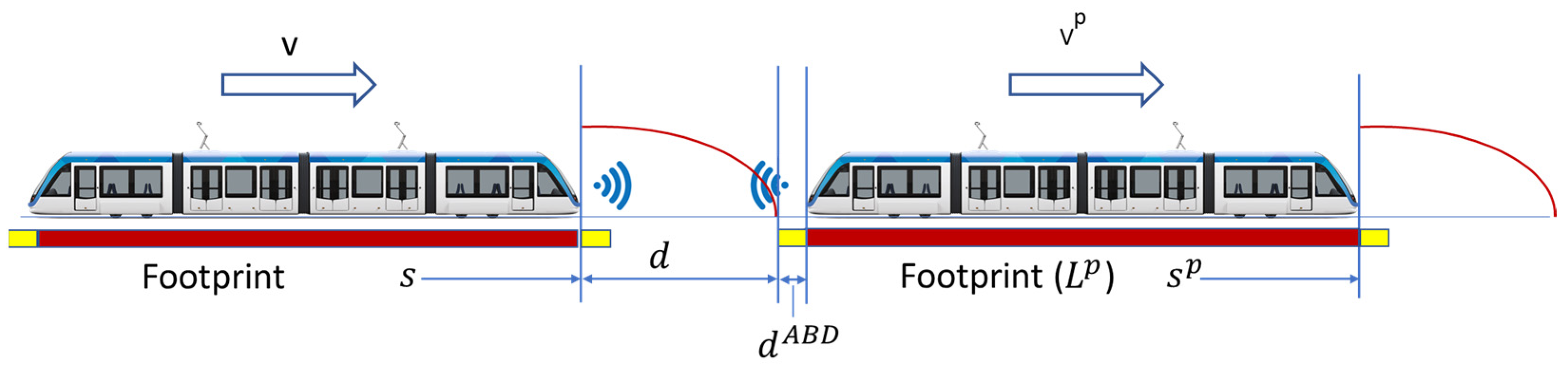Figure 1 represents the inter-train distance ($d$) and the inter-train distance considering the ABD ($d^{ABD}$).

Note that, while $s_{k|t}$ and $v_{k|t}$ are calculated by the controller and $L^p$ and $b$ are introduced as constant input parameters, variable $s^p$ in Equation (3) is introduced as input data at each time the controller is executed. At the beginning of the prediction horizon ($k=t$), $s^p$ contains the last known current position of the in-front train, whereas it contains estimated positions of the in-front train for the rest of the prediction horizon. These estimations are obtained by using Equation (2) with the last known current control force $u$ applied by the in-front train, which is considered to remain constant throughout the complete prediction horizon estimation, and departing from the last known current position of the in-front train considered for $k=t$.

3. LMPC Formulation

This section is dedicated to the proposed LMPC’s formulation and is divided into four subsections. The first and second subsections are committed to the explanation of the two main components of the proposed LMPC’s optimization problem: the control policy and the learning policy, respectively. The third subsection gathers the first and second subsections and presents the complete optimization problem of the proposed LMPC. Finally, a fourth subsection closes the section by presenting the learning index that is used to assess whether the proposed LMPC converges after several iterations of learning.

3.1. LMPC’s Control Policy

The proposed LMPC’s control policy consists of those cost terms and constraints of the optimization problem that do not implement a learning policy; i.e., those optimization problem’s elements that might be also part of a conventional MPC when calculating the decision variable $u$. Specifically, the proposed LMPC’s control policy consists of the optimization problem’s initialization constraint, the dynamics constraint, the decision variable constraints, the speed constraints, the inter-train distance constraints, and the control policy’s cost terms. All these components are explained in the following.

First, regarding the initialization constraint, the state vector $x$ is initialized with the real running conditions, which are introduced to the controller as input data. This way, the LMPC’s optimization problem can calculate the decision variable $u$ while considering the train’s current operational situation. Hence, in Equation (4), the first time step $k$ within the prediction horizon $H_p$ is constrained so that its values are coincident to the real running conditions $x\left(t\right)$:

$$x_{k|t}=x\left(t\right)\hspace{1em}k=t$$

(4)

Once the first time step has been initialized, the following time steps of the state vector’s values are determined by the dynamics constraint, which is defined in terms of the state equation—Equation (2). As this equation depends on the decision variable $u$, which is calculated by the optimization problem, the subsequent time steps of the state vector depend on the calculated values for $u$. However, when calculating these time steps, the state vector and the decision variable $u$ must also fulfill the decision variable constraints, the speed constraints, and the inter-train distance constraints.

The decision variable constraints are given by the set $\mathcal{U}$ in Equation (5), which is a group of constraints consisting of four types of constraints given in the subsets ${\mathcal{U}}_1$, ${\mathcal{U}}_2$, ${\mathcal{U}}_3,$ and ${\mathcal{U}}_4$. The first type of the decision variable constraints is given by ${\mathcal{U}}_1$, in which a control horizon is set. This means that the decision variable $u$ is only calculated from the first time step to the control horizon ($H_c$), while, from the first time step after the control horizon to the time step that corresponds to the prediction horizon’s end, the decision variable $u$ is not calculated. Instead, from the first time step after the control horizon, the decision variable is maintained constant and its values must be equal to the decision variable’s last calculated value in the prediction horizon, which corresponds to the control horizon’s time step.

The second and third types of the decision variable constraints are given by ${\mathcal{U}}_2$ and ${\mathcal{U}}_3$, in which the decision variable $u$ is constrained in terms of the maximum force ($u_{max}$) and power ($P_{max}$), respectively. This way, the traction and braking curves are implemented in the LMPC’s optimization problem. Similarly, in ${\mathcal{U}}_4$, the longitudinal jerk, given by the first element of the output vector ($y^1$) and defined in Equation (3), is constrained for traction and braking in terms of the maximum allowed jerk ($j_{max}$). Thus, this last constraint enhances comfort by reducing the decision variable’s oscillations:

$$\mathcal{U}={\displaystyle {\bigcap }_p^4}{\mathcal{U}}_p, being\left\{\begin{array}{l}{\mathcal{U}}_1=\left\{u_{k|t}:u_{k+1|t}-u_{k|t}=0\right\}\\ {\mathcal{U}}_2=\left\{u_{k|t}:-u_{max}\le u_{k|t}\le u_{max}=0\right\}\\ \begin{array}{l}{\mathcal{U}}_3=\left\{u_{k|t}:-P_{max}\le u_{k|t}·v_{k|t}\le P_{max}=0\right\}\\ {\mathcal{U}}_4=\left\{u_{k|t}:-j_{max}\le y_{k|t}^1\le j_{max}=0\right\}\end{array}\end{array}\right.\begin{array}{l}k=H_c,\dots ,H_p-1\\ k=t,\dots ,H_p\\ \begin{array}{l}k=t,\dots ,H_p\\ k=t,\dots ,H_p-1\end{array}\end{array}$$

(5)

The abovementioned speed constraints are given by the set $\mathcal{V}$ in Equation (6), which gathers a group of three types of constraints given by the subsets ${\mathcal{V}}_1$, ${\mathcal{V}}_{2,}$ and ${\mathcal{V}}_3$. The first type of the speed constraints is given by ${\mathcal{V}}_1$, in which the speed is constrained to remain below the reference speed curve ($v_{ref}$), i.e., the maximum speed that the train is capable of reaching, always respecting the maximum speed limits set for the line. This reference speed curve is calculated offline taking into account the line and train’s characteristics according to the dynamic programming algorithm described in [37] and it is part of the input data introduced to the controller. Moreover, the second type of speed constraints is given by ${\mathcal{V}}_2$, in which the speed is constrained to remain above a constant value. Furthermore, the third type of speed constraints is given by ${\mathcal{V}}_3$, in which reversing is prohibited. Note that ${\mathcal{V}}_3$ is necessary to avoid any chance of reversing because ${\mathcal{V}}_2$ is defined as a soft constraint through the slack variable ${\zeta }_{k|t}^{v_{min}}$:

$$\mathcal{V}={\displaystyle {\bigcap }_p^3}{\mathcal{V}}_p, being\left\{\begin{array}{l}{\mathcal{V}}_1=\left\{v_{k|t}:v_{k|t}-{\zeta }_{k|t}^{v_{max}}\le v_{ref}\left(s_{k|t}\right),{\zeta }_{k|t}^{v_{max}}\ge 0\right\}\\ {\mathcal{V}}_2=\left\{v_{k|t}:v_{min}\le v_{k|t}+{\zeta }_{k|t}^{v_{min}},{\zeta }_{k|t}^{v_{min}}\ge 0\right\}\\ {\mathcal{V}}_3=\left\{v_{k|t}:v_{k|t}\ge 0\right\}\end{array}\right.\begin{array}{l}k=t,\dots ,H_p\\ k=t,\dots ,H_p\\ k=t,\dots ,H_p\end{array}$$

(6)

The inter-train distance constraints are given by the set $\mathcal{D}$ in Equation (7), which is a group of constraints consisting of three types of constraints given in the subsets ${\mathcal{D}}_1$, ${\mathcal{D}}_2,$ and ${\mathcal{D}}_3$. The first type of the inter-train distance constraints is given by ${\mathcal{D}}_1$, in which the ABD, which also implements the moving block as seen in Equation (3), is constrained to remain above the desired distance $d_{des}$ used as a control policy’s objective. Moreover, the second type of inter-train distance constraints is given by ${\mathcal{D}}_2$, in which the ABD is also constrained to remain above the desired distance $d_{des}$ at the end of the prediction horizon, as a terminal constraint. In addition, the inter-train distance, as defined in Equation (3), is constrained above the minimum safe distance $d_{min}$ in the additional terminal constrain given by ${\mathcal{D}}_3$:

$$\mathcal{D}={\displaystyle {\bigcap }_p^3}{\mathcal{D}}_p, being\left\{\begin{array}{l}{\mathcal{D}}_1=\left\{y_{k|t}^3:d_{des}\le y_{k|t}^3+{\zeta }_{k|t}^{y^3},{\zeta }_{k|t}^{y^3}\ge 0\right\}\\ {\mathcal{D}}_2=\left\{y_{k|t}^3:d_{des}\le y_{H_p+1|t}^3+{\zeta }_{H_p+1|t}^{y^3},{\zeta }_{H_p+1|t}^{y^3}\ge 0\right\}\\ {\mathcal{D}}_3=\left\{y_{k|t}^2:d_{min}\le y_{H_p+1|t}^2+{\zeta }_{H_p+1|t}^{y^2},{\zeta }_{H_p+1|t}^{y^2}\ge 0\right\}\end{array}\right.k=t,\dots ,H_p$$

(7)

Finally, the control policy’s cost ($J_C$) is defined in Equation (8), which is only a part of the optimization problem’s complete cost function. As seen in Equation (8), the control policy’s cost is defined differently depending on whether the LMPC is controlling a leading train or a following train. For this paper’s purpose, the leading train ($n=1$) is defined as a train that moves without inter-train constraints because it does not have any train in front, whereas the following train ($n>1$) is defined as the train that follows the leading train, or other following trains, and that moves considering the inter-train constraints due to the proximity of the trains moving in front. Thus, the leading train’s control policy is determined by the deviation from the reference speed profile ($J_v$), whose objective is a maximum speed control policy. Note that these cost terms are normalized by the train’s maximum speed ($v_{max}$). On the contrary, the following train’s control policy is determined by the deviation of the inter-train distance from the desired distance ($d_{des}$), which also normalizes these cost terms. In addition, the following train’s control policy takes into account the slack variables related to the inter-train distance constraints explained in Equation (7). Hence, the following train’s control policy is a minimum distance control policy constrained by the moving block inter-train distance constraints. Moreover, both the leading and the following trains share common cost terms, which are given by $J_{u-\zeta }$, related to the longitudinal jerk’s minimization and the slack variables for Equation (5):

$$J_C\left(x_{k|t},u_{k|t}\right)=\left\{\begin{array}{l}{J}_{u-\zeta }+J_v\\ J_{u-\zeta }+J_y\end{array}\right.\begin{array}{c}n=1\\ n>1\end{array}$$

(8)

being

$$\begin{array}{l}{J}_v={\displaystyle \sum _{k=1}^{k=H_p-1}}{\left({\displaystyle \frac{v_{k+1|t}-v_{ref}\left(s_{k+1|t}\right)}{v_{max}}}\right)}^2\\ J_y={\displaystyle \sum _{k=1}^{k=H_p}}\left|{\displaystyle \frac{d_{k+1|t}-d_{des}}{d_{des}}}\right|+{\displaystyle \sum _{k=1}^{k=H_p+1}}\left({\displaystyle \frac{{\zeta }_{k|t}^{y^3}}{d_{des}}}\right)+{\displaystyle \frac{{\zeta }_{H_p+1|t}^{y^2}}{d_{des}}}\\ J_{u-\zeta }={\displaystyle \sum _{k=1}^{k=H_p-1}}{\left({\displaystyle \frac{y_{k|t}^1}{j_{max}}}\right)}^2+{\displaystyle \sum _{k=1}^{k=H_p}}\left({\displaystyle \frac{{\zeta }_{k|t}^{v_{min}}}{v_{max}}}+{\displaystyle \frac{{\zeta }_{k|t}^{v_{max}}}{v_{max}}}\right)\end{array}$$

3.2. LMPC’s Learning Policy

The proposed LMPC learning policy consists of those cost terms and constraints of the optimization problem that do implement a learning policy, and therefore, the elements of the optimization problem that calculate the decision variable $u$ using data from past experiences. Specifically, the proposed LMPC’s learning policy is implemented through the terminal constraint on speed, as well as the cost terms of the learning policy.

The terminal constraint on speed is given by the set ${\mathcal{V}}_L$ in Equation (9), where the speed is constrained between the real speeds reached at the same track’s point in past iterations. Thus, the speed is constrained to strike a balance between the real speeds that eventually happened during previous iterations by means of the learning variable $\lambda$, which weights the considered past iterations. These real speeds are also introduced to the controller by means of the optimization problem’s variable $v^{\lambda }$, as well as their cost evaluated in terms of Equation (8) in the variable $Q_f$. Therefore, variables $v^{\lambda }$ and $Q_f$ are used to consider the controller’s input data related to learning:

$${\mathcal{V}}_L=\left\{v_{H_p+1|t}:v_{H_p+1|t}=v_{·|t}^{\lambda }\left(s_{·|t}\right)·{\lambda }_{·|t},{\lambda }_{·|t}\ge 0,\sum {\lambda }_{·|t}=1\right\}$$

(9)

In Equation (9), variable $v^{\lambda }$ is a row vector with $r·(H_p+1)$ columns, where $r$ represents the iteration in which the LMPC is being executed. As far as this paper is concerned, an ‘iteration’ must be understood as the travel of the line’s entire length. Hence, the train must run the complete line with several iterations, so that the LMPC can be trained, and the completely trained LMPC can use all past iterations in order to improve the train’s repetitive behavior on the line. From these past iterations, the LMPC uses the data concerning a prediction of the horizon’s length from the current train’s position at each iteration, leading to the $r·(H_p+1)$ column dimension. For this reason, in ‘$·|t$’, the dot represents a different number of time steps depending on the iteration’s number, according to the aforementioned $r·(H_p+1)$ column dimension.

Finally, the learning policy’s cost ($J_L$) is defined in Equation (10), which is only a part of the optimization problem’s complete cost function. This learning policy’s cost depends on the learning variable and the cost of the input data from previous iterations, optimizing the repetitive behavior of a train on a given track and line:

$$J_L\left({\lambda }_{·|t}\right)=Q_f\left(s_{·|t}\right)·{\lambda }_{·|t}$$

(10)

3.3. LMPC’s Complete Optimization Problem Formulation

Having seen the controller’s control and learning policies, the complete formulation for the LMPC’s optimization problem can be given as in Equations (11)–(13):

$$\underset{u_{·|t}}{\min }{J}_T\left(x_{k|t},u_{k|t},{\lambda }_{k|t}\right)$$

(11)

subject to

$$\begin{array}{c}{x}_{t|t}=x\left(t\right)\\ x_{k+1|t}=x_{k|t}+t_s{\dot{x}}_{k|t} \\ \begin{array}{c}{u}_{k|t}\in \mathcal{U}\\ v_{k|t}\in \mathcal{V}\\ y_{k|t}^{\mathrm{2,3}}\in \mathcal{D}\end{array}\end{array}\begin{array}{l}\forall n\in N\\ \forall n\in N\\ \begin{array}{l}\forall n\in N\\ \forall n\in N\\ \forall n\in N\backslash \left\{1\right\}\end{array}\end{array}$$

(12)

where

$$J_T\left(x_{k|t},u_{k|t},{\lambda }_{k|t}\right)=J_C\left(x_{k|t},u_{k|t}\right)+J_L\left({\lambda }_{·|t}\right)$$

(13)

This optimization problem is independently applied to and individually solved on each train, which is denoted by $n=\mathrm{1,2},\dots ,N$, $N$ being the total of the trains running on the line and that are being controlled by independent LMPCs for each train. Thus, at each time instant ($t$), each train computes the decision variable according to its optimization problem and applies the first time step of the calculated prediction horizon ($u_{1|t}$). This approach makes this optimization problem scalable, since its computation time does not depend on the number of trains running on the line and that are being controlled by independent LMPCs for each train ($N$). Moreover, the feasibility, stability, and learning convergence proofs of the proposed LMPC were treated in a general theoretical proof in [38,39].

3.4. Learning Index

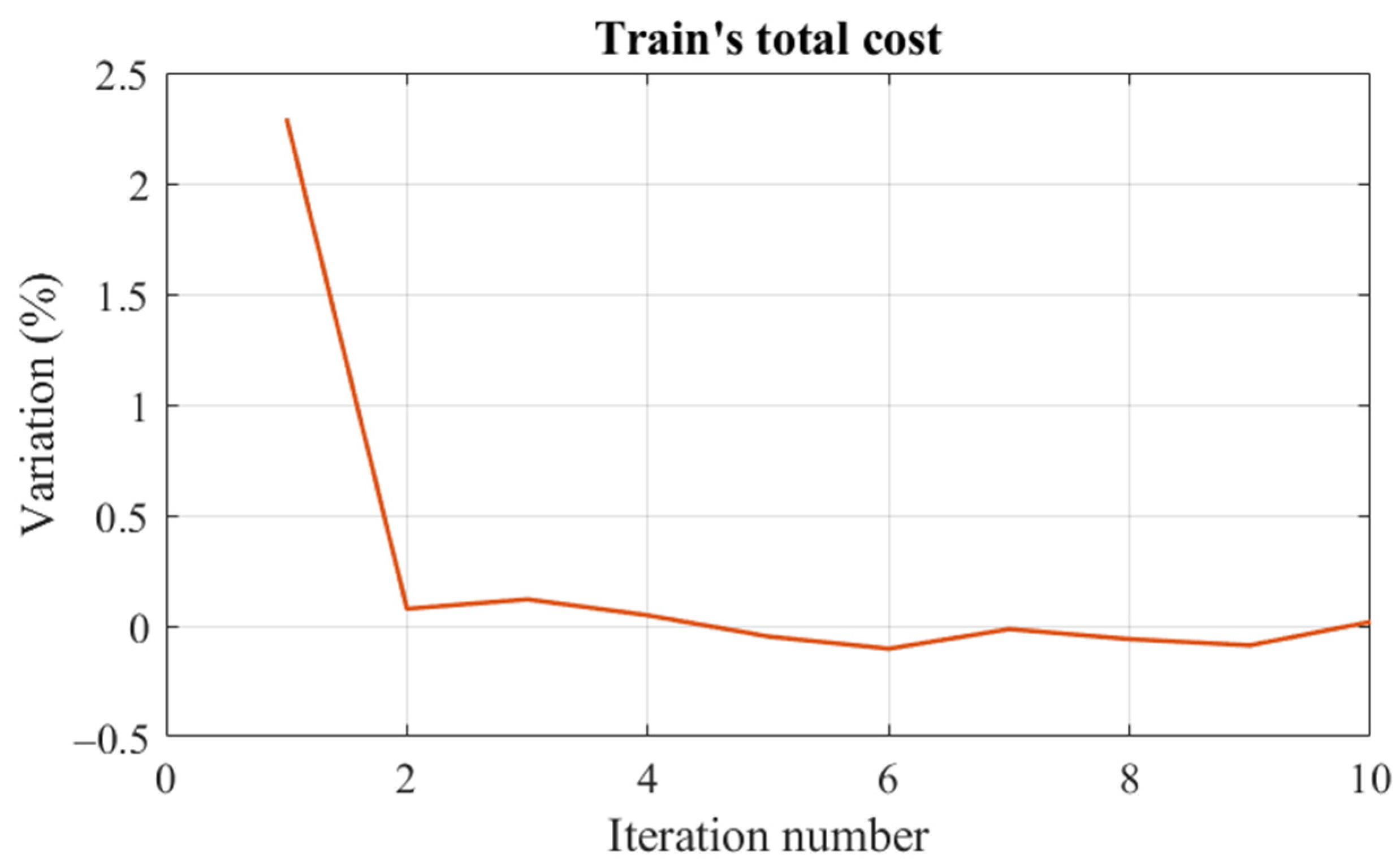
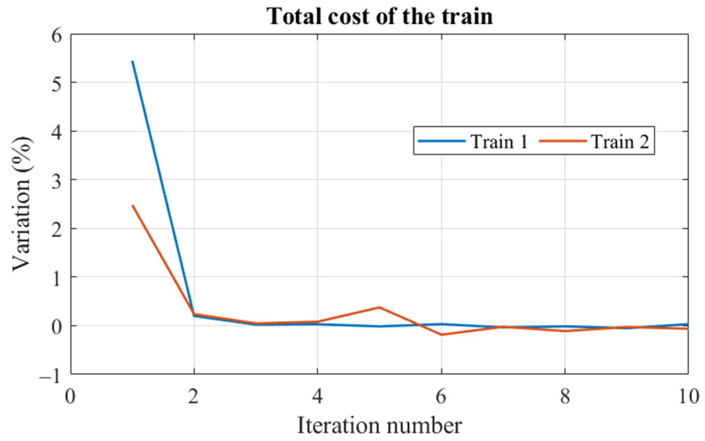
The learning index ($LI$) measures whether the proposed LMPC converges after several iterations of learning. Measured in percentage units for each train in which the proposed LMPC is applied to, its formulation is based on the relative variation of the average value of the control policy’s cost, as defined in Equation (8), from the iteration evaluated with respect to the previous iteration. Hence, the iterations are considered to have converged when this metric approaches zero in a steady state:

$$L{I}_n^r\left(\%\right)={\displaystyle \frac{J_{C,n}^r-J_{C,n}^{r-1}}{J_{C,n}^{r-1}}}·100$$

(14)

where $L{I}_n^r$ is the learning index for the $n$-train in the $r$-iteration, measured in percentage units, and $J_{C,n}^r$ is the control policy cost’s average value for train $n$ in iteration $r$.

Note also that the $LI$ is a metric which is defined and used outside the optimization problem formulation for assessing the LMPC’s convergence after several iterations.

4. Simulations and Results

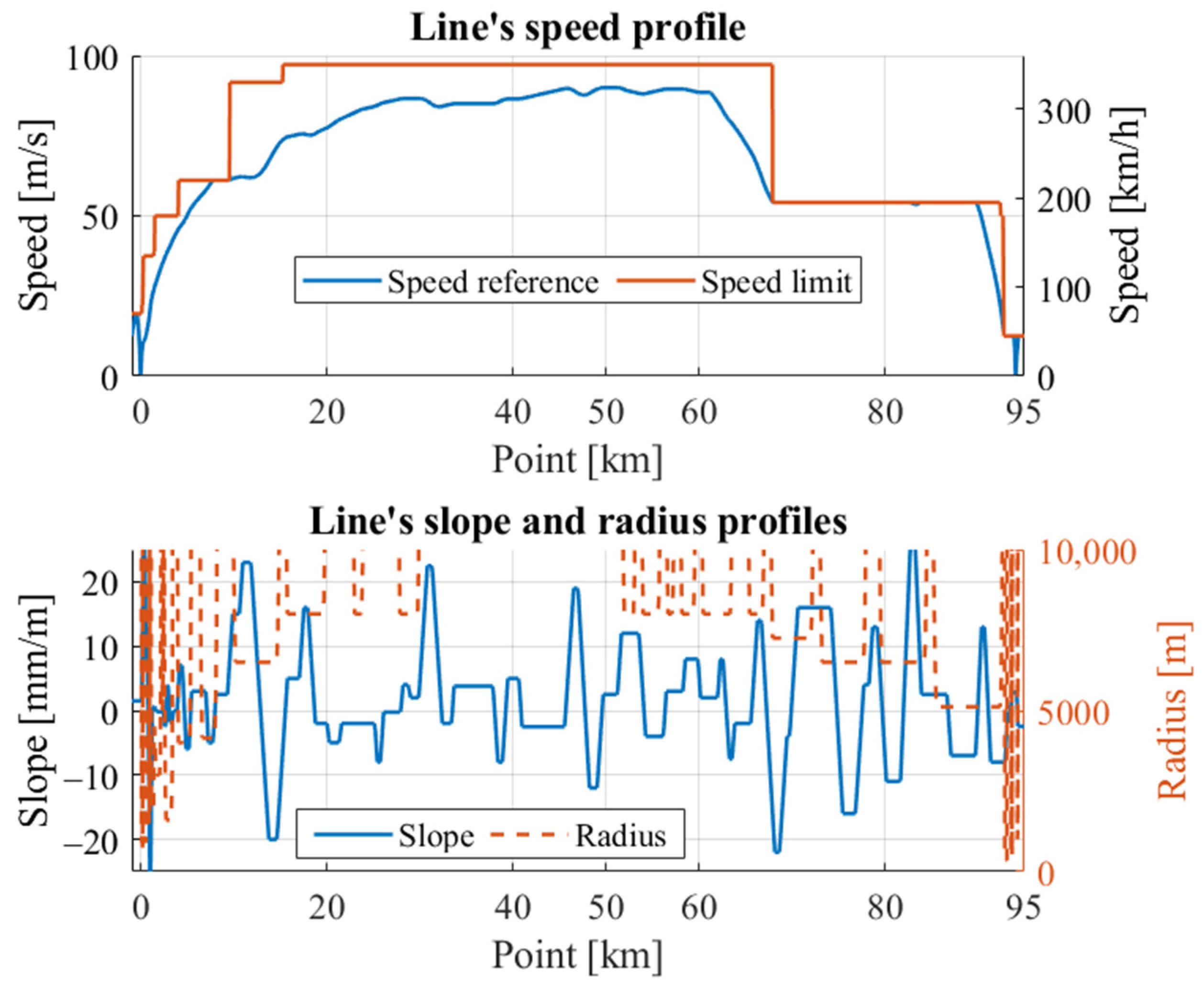
This section simulates the proposed LMPC for a high-speed line under the moving block principle. The high-speed train has the characteristics specified in Table 1, whereas the high-speed line’s speed and track profiles are shown in Figure 2, in which a negative slope represents downhill in the train’s direction of movement.

The simulations consider two trains running closely and simultaneously on the track. The first train passing over a kilometer point is denoted as the ‘leading train’ and it is supposed to move without inter-train distance constraints because it does not have any train in front. It is also supposed to move without any signaling limitations derived from red light signals, and it tracks a reference speed profile, implementing a maximum speed control policy. Hence, it corresponds to the LMPC’s formulation for $n=1$. The second train passing over a kilometer point is denoted as the ‘following train’ and it is supposed to move under inter-train distance constraints due to the proximity of a train moving in front. Therefore, this train is constrained by the moving block signaling principle and it implements a moving block minimum distance control policy. Hence, the following train corresponds to the LMPC’s formulation for $n>1$.

Thus, both trains allow the simulations to assess the complete formulation of the proposed LMPC. They also allow the LMPC’s performance assessment under two moving block scenarios: large inter-train distances (given by the leading train) and short inter-train distances (given by the following train). These operational situations might happen on lines with varying frequencies [40,41].

The simulations are divided into two distinct simulation cases: simulation F and simulation L + F. In Simulation F, the LMPC is only used in the following train, while the leading train uses a conventional non-learning MPC, as in [42]. This simulation also assesses the compatibility of the proposed LMPC with other non-learning controllers, apart from the LMPC’s behavior when applied to the following train. In Simulation L + F, the LMPC is used by both types of trains: the leading train and the following train. Therefore, apart from assessing the LMPC’s behavior in the leading and following trains, this simulation also assesses the compatibility of the proposed LMPC when applied to several trains simultaneously.

In order to compare the simulation results and assess the proposed LMPC’s performance, the following variation indexes were used: the variation in absolute terms ($\Delta \alpha$) and the variation in relative terms (${\Delta }_{\mathrm{\%}}\alpha$):

$$\begin{array}{c}\Delta \alpha ={\alpha }_{LMPC}-{\alpha }_{MPC}\\ {\Delta }_{\mathrm{\%}}\alpha ={\displaystyle \frac{{\alpha }_{LMPC}-{\alpha }_{MPC}}{{\alpha }_{MPC}}}·100\end{array}$$

(15)

where ${\alpha }_{LMPC}$ and ${\alpha }_{MPC}$ are denoted as generic variables, the variables whose variation is being compared. ${\alpha }_{MPC}$ represents the variable’s value when using the conventional non-learning MPC in [42], whereas ${\alpha }_{LMPC}$ denotes the variable’s value when using the proposed LMPC.

Finally, the results presented in this paper were obtained in a Windows 11, i7-1365U 1.8 GHz CPU, 32 GB RAM platform using MATLAB (R2021b Update 7), the YALMIP interface (R20210331) [43], and the IPOPT solver (v3.12.9) [44].

4.1. Simulation F

In Simulation F, the LMPC is only used in the following train, while the leading train uses a conventional non-learning MPC, as in [42]. Thus, apart from assessing the LMPC’s behavior when applied to the following train, this simulation also assesses the compatibility of the proposed LMPC with other non-learning controllers.

The simulation is analyzed from two perspectives. From the first perspective, the obtained results for the simulated LMPC are analyzed. From the second perspective, the obtained results are compared with an equivalent operation under a conventional non-learning MPC in the following train, instead of the LMPC, and the results are further discussed.

4.1.1. LMPC’s Results for the Following Train

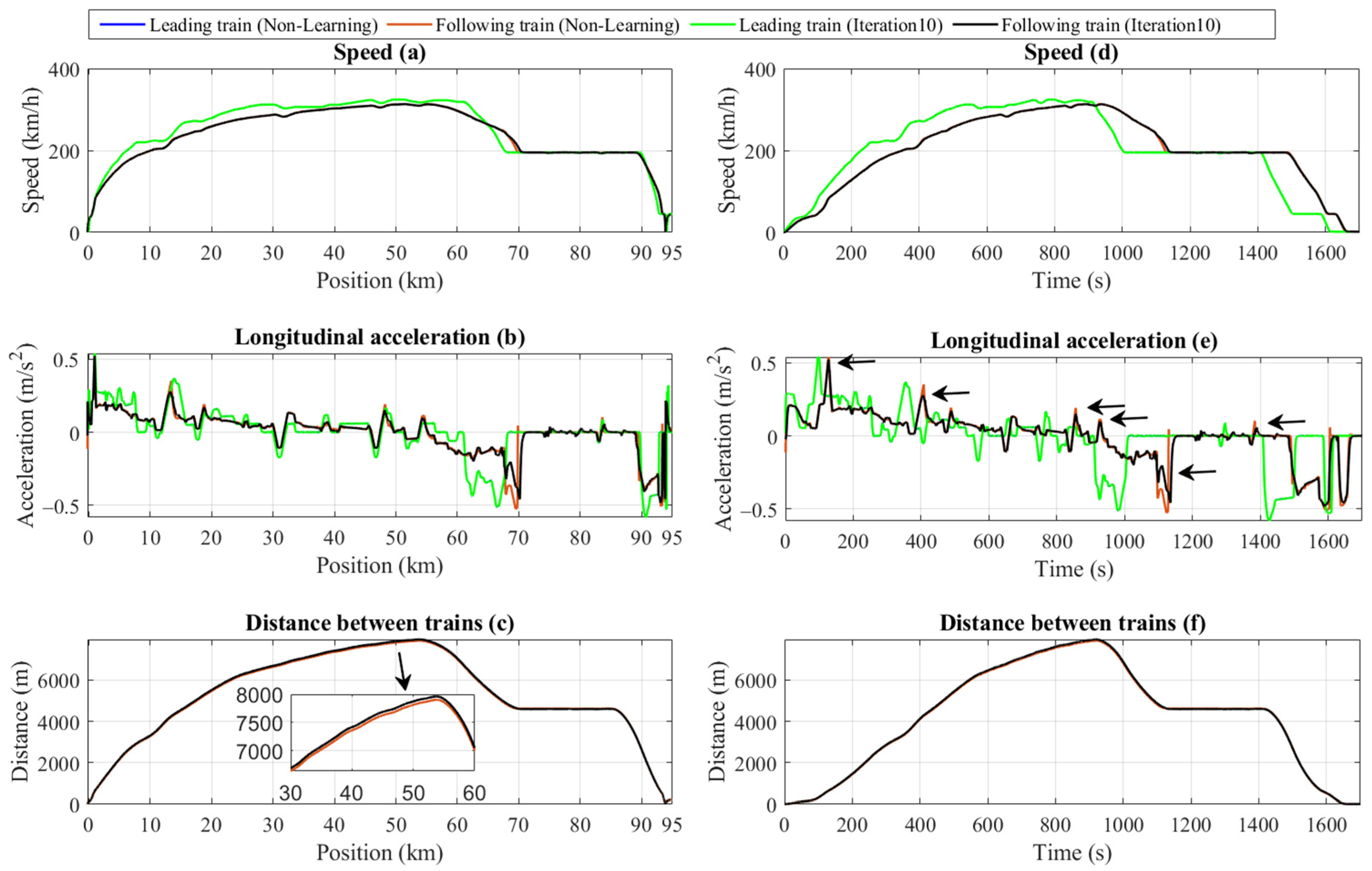
Figure 3 shows the obtained results for the following train, labelled as ‘Following train (Iteration 10)’, regarding the speeds, accelerations and decelerations, and the inter-train distances throughout the length of the line. The speed limitations are fulfilled. Accelerations and decelerations remain within the traction and braking limitations, given by the train’s characteristics and included in the optimization problem’s constraints. Inter-train distances are minimized while fulfilling the moving block principle for train separation, and therefore, ensuring safety.

Table 2. Simulation results for the proposed LMPC and a conventional non-learning MPC. Variations in the variables’ values.

Variable	MPC: Following Train	Simulation F: Following Train	Simulation L + F: Following Train	Simulation L + F: Leading Train	MPC: Leading Train
Maximum inter-train distance (m)	7902.7	7961.4	7980.7
Minimum inter-train distance (m)	10.0	10.0	10.0
Force average (kN)	47.4	46.1	46.1	47.3	47.4
Energy consumption (kWh)	1745.44	1722.39	1722.19	1906.06	1910.78
Specific energy consumption (kWh/vehicle·km)	2.32	2.29	2.29	2.53	2.54

summarizes the train’s energy consumption, in which a lower consumption can be observed for the following train than in the leading train, and where no energy savings derived from regenerative braking have been included. However, note that this difference is due to the different control policies applied to each train and not because of the application of a learning or non-learning controller to a train, as can be concluded from the Simulation L + F. Thus, the leading train presents a larger energy consumption because it follows a maximum speed control policy, whereas the following train, which follows a minimum distance policy, is limited by the moving block constraints, preventing the following train from achieving the same maximum speeds and accelerations as the leading train does, and therefore, leading to a lower energy consumption. This last affirmation can be seen in the speed plot in Figure 3.

Figure 4 represents the learning index’s evolution over several iterations, in which it can be seen that the LMPC converges by the 7th iteration. In addition,

Table 3. Computation times comparison between the proposed LMPC and the conventional non-learning MPC.

Variable	Train	MPC	Simulation F	Simulation L + F
Total computation time (s)	Leading train	454.1		576.7 (+27.0%)
	Following train	457.9	560.9 (+22.5%)	567.4 (+23.9%)

shows that the LMPC’s total computation time is 560.9 s for a simulation of 1856.0 s, which demonstrates that the proposed LMPC can be used for online applications that need a real-time execution.

4.1.2. LMPC Comparison with a Conventional Non-Learning MPC in Simulation F

Under the ‘Following train (Iteration 10)’ label, Figure 3 shows that the obtained results for the following train are close to the results obtained with the equivalent conventional MPC, which is labeled as ‘Following train (MPC)’. The arrows in Figure 3 indicate relevant points at which the accelerations and decelerations are softened in LMPC with respect to the non-learning MPC.In this comparison, it can be seen that the results are similar in terms of speeds, accelerations, distance between trains, and travel times. In fact, the distance between the trains has only increased by 58.7 m (+0.7%), which is less than the train’s length.

In this figure, note also that the plots concerning the leading train, labeled as ‘Leading train (Non-learning)’ and ‘Leading train (Iteration 10)’, are coincident because they represent the same conventional non-learning MPC, since the leading train is not using the proposed LMPC in this simulation.

In addition,

Table 4. Simulation results for the proposed LMPC with respect to a conventional non-learning MPC. Variations in the variables’ values.

Variable’s Variation	Simulation F: Following Train	Simulation L + F: Following Train	Simulation L + F: Leading Train	Simulation L + F: Leading + Following Trains
Maximum inter-train distance (m)	58.7 (+0.7%)	78.0 (+1.0%)
Minimum inter-train distance (m)	0.0 (0.0%)	0.0 (0.0%)
Force average (kN)	−1.3 (−2.8%)	−1.4 (−2.9%)	−0.1 (−0.3%)
Energy consumption (kWh)	−23.06 (−1.3%)	−23.25 (−1.3%)	−4.72 (−0.2%)	−27.97 (−0.8%)
Specific energy consumption (kWh/vehicle·km)	−0.03 (−1.3%)	−0.03 (−1.3%)	−0.01 (−0.2%)	−0.04 (−0.8%)

indicates that the energy consumption is reduced by 23.06 kWh (0.03 kWh/vehicle·km, (−1.3%)) in LMPC with respect to the conventional non-learning MPC. Despite the low reductions in the traction force average (Table 4), Figure 3 reveals that accelerations and decelerations are softened, which explains that the energy consumption reduction is due to an optimization of the train’s control forces in LMPC with respect to a conventional non-learning MPC by means of the jerk’s cost term (that is reduced by 63%). Note that this cost term is optimized further than other cost terms because, based on past iteration data, it can be concluded that reference tracking and constraint fulfillment can be maintained with other local solutions in which less power is used because braking is needed within a short distance. Other cost terms are not further optimized due to competing improvements: the constraints’ slack optimization might lead to poor reference tracking, whereas the reference tracking’s optimization might lead to constraint violations.

4.2. Simulation L + F

In Simulation L + F, the LMPC is used by both trains: the leading train, which moves without inter-train constraints because it does not have any train in front, and the following train that follows the leading train, which does move with inter-train constraints due to the proximity of the leading train moving in front. Thus, apart from assessing the LMPC’s behavior when applied to the leading and following trains, this simulation also assesses the compatibility of the proposed LMPC when it is applied simultaneously to other trains running on the line.

The simulation is analyzed from two perspectives. From the first perspective, the obtained results for the simulated LMPC are analyzed. From the second perspective, the obtained results are compared with an equivalent operation under a conventional non-learning MPC in all trains, instead of the LMPC applied to each train, and the results are further discussed.

4.2.1. LMPC’s Results for the Leading and Following Trains

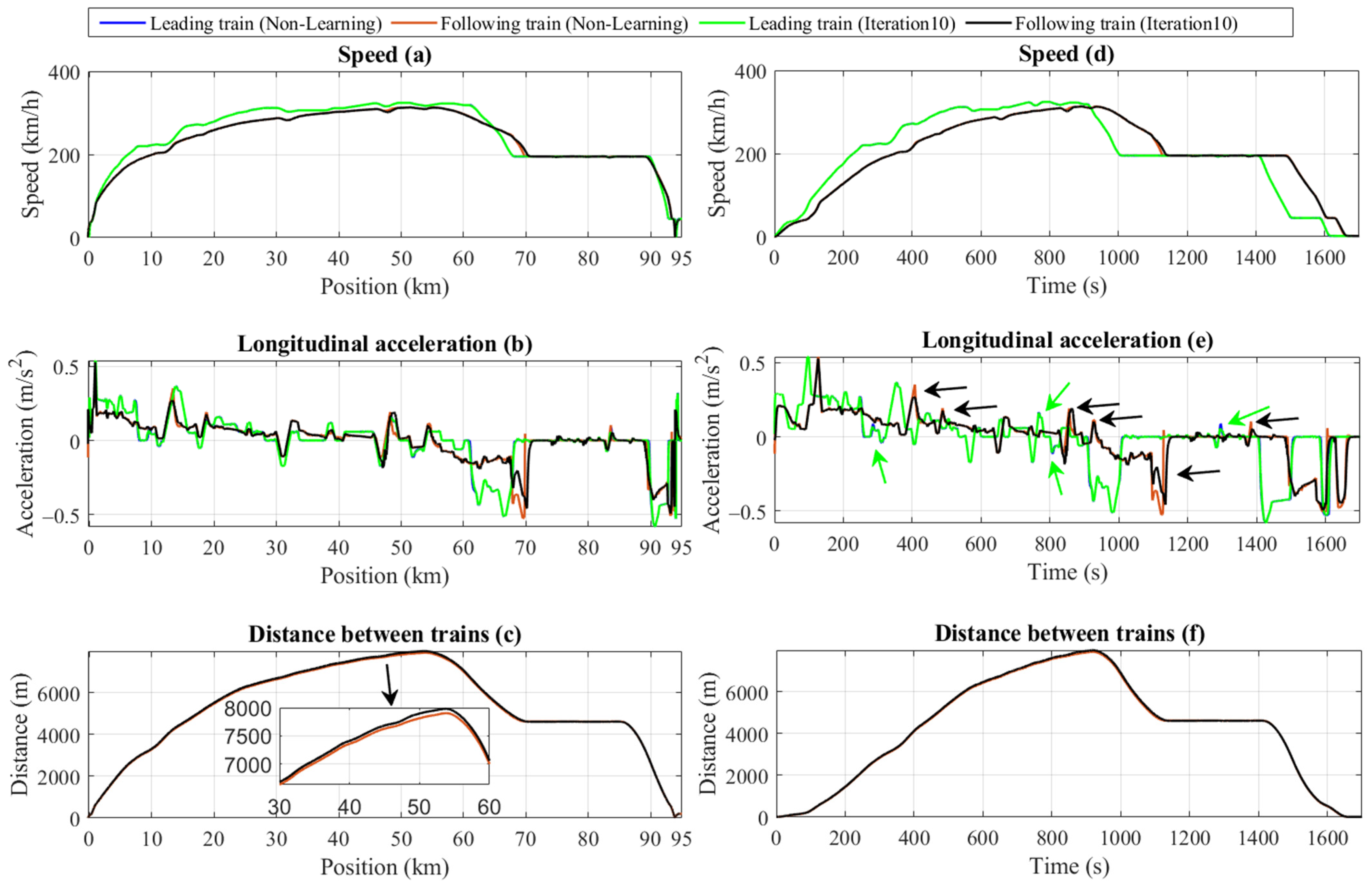
Figure 5 shows the obtained results for the leading and following trains when applying the proposed LMPC, labelled as ‘Leading train (Iteration 10)’ and ‘Following train (Iteration 10)’, respectively. In this figure, the following results are provided for both trains: speeds, accelerations and decelerations, and the inter-train distances throughout the length of the line. The results are similar to Simulation F: speed limitations are fulfilled for both trains. Accelerations and decelerations remain within the traction and braking limitations for both trains, given by the train’s characteristics and included in the optimization problem’s constraints. As in Simulation F, inter-train distances are minimized while fulfilling the moving block principle for train separation and, therefore, ensuring safety.

Table 2 summarizes the train’s energy consumption, in which a lower consumption can be observed for the following train than in the leading train and where no energy savings derived from regenerative braking have been included. However, note that this difference is due to the different control policies applied to each train and not because of the application of a learning or non-learning controller to a train, as can be concluded from the Simulation L + F. Thus, the leading train presents a larger energy consumption because it follows a maximum speed control policy, whereas the following train, which follows a minimum distance policy, is limited by the moving block constraints, preventing the following train from achieving the same maximum speeds and accelerations as the leading train does, and therefore, leading to a lower energy consumption. This last affirmation can be seen in the speed plot in Figure 5.

Figure 6 represents the learning index’s evolution over several iterations, in which it can be seen that the LMPC converges by the 3rd iteration for the leading train and the 7th iteration for the following train. In addition, Table 3 outlines that the LMPC’s total computation time is 576.7 s and 567.4 s for the leading and the following train, respectively, and for a simulation of 1856.0 s, which demonstrates that the proposed LMPC can be used for online applications that require a real-time execution.

4.2.2. LMPC Comparison with a Conventional Non-Learning MPC in Simulation L + F

Under the ‘Leading train (Iteration 10)’ and ‘Following train (Iteration 10)’ labels, Figure 5 shows that the obtained results for all trains are close to the results obtained with the equivalent conventional MPC, which are labeled as ‘Leading train (MPC)’ and ‘Following train (MPC)’, respectively. In this comparison, it can be seen that the results are similar in terms of speeds, accelerations, distance between trains, and travel times. In fact, the distance between trains is only increased by 78.0 m (+1.0%), which is less than the train’s length.

In Figure 5, note also that the plots concerning the leading train, labeled as ‘Leading train (Non-learning)’ and ‘Leading train (Iteration 10)’, do not completely overlap because the leading train is using the proposed LMPC in this simulation, and therefore, they do not represent the same controller, as in Simulation F. The arrows in Figure 5 indicate relevant points at which the accelerations and decelerations are softened in LMPC with respect to the non-learning MPC.

In addition, Table 4 indicates that the energy consumption is reduced by 27.97 kWh (0.04 kWh/vehicle·km, (−0.8% average)) for the sum of the two trains in LMPC with respect to the conventional non-learning MPC. This reduction is mainly due to the following train’s energy consumption reduction of 23.25 kWh (0.03 kWh/vehicle·km, (−1.3% in the following train)), compared with the leading train’s energy consumption reduction of 4.72 kWh (0.01 kWh/vehicle·km, (−0.2%)) in LMPC with respect to the conventional non-learning MPC. Compared with Simulation F, this total energy consumption reduction is larger because the LMPC is also applied to the leading train, not only to the following train; i.e., as the LMPC is applied to more trains, the energy consumption increases.

Despite the low reductions in the traction force average (Table 4), Figure 5 reveals that accelerations and decelerations are softened, which explains that the energy consumption reduction is due to an optimization of the train’s control forces in LMPC with respect to a conventional non-learning MPC by means of the jerk’s cost term, as in Simulation F. In fact, the jerk’s average is reduced by 33% for the leading train and by 106% for the following train, in line with the energy consumption reductions. Note that this cost term is optimized further than other cost terms because, based on past iterations’ data, it can be concluded that reference tracking and constraint fulfillment can be maintained with other local solutions in which less power is used because braking is needed within a short distance. Other cost terms are not further optimized due to competing improvements: the constraints’ slack optimization might lead to poor reference tracking, whereas the reference tracking’s optimization might lead to constraint violations.

4.3. Further Discussion

Hence, Simulations F and L + F reveal that the following train’s results when applying the proposed LMPC are acceptable whether the leading train is also using the proposed LMPC or not. This fact allows the application of the proposed LMPC to the following train in an autonomous way, the simultaneous application of the proposed LMPC to the leading train not being a requisite for an acceptable performance of the following train when using the LMPC. In any case, once the trains using LMPC have been trained, they optimize their repetitive behavior on the line thanks to the proposed LMPC.

Moreover, being on the same order of magnitude, these energy consumption reductions are comparable in magnitude to other labor-intensive measures currently being implemented in the rail sector, such as the ones considered in [45,46], including solar panels installation. To illustrate this affirmation, the obtained 1.3% reduction in the energy consumption would lead to a 14 GWh/year energy consumption reduction in the Italian network, whose energy consumption dedicated to high-speed traction was 1077.5 GWh in 2024 [47]. Considering the European Union dwellings’ annual electricity consumption of 3.7 MWh/(year dwelling) [48], the achieved energy savings are equivalent to the yearly electricity consumption of approximately 3786 dwellings in a network such as the Italian high-speed rail system, obtained through a simple modification of the train control software from the abovementioned conventional non-learning MPC to the proposed LMPC. In economic terms, assuming an average electricity price of €0.20/kWh, these energy savings correspond to approximately €2.8 million per year.

Furthermore, the compared controllers (the proposed LMPC and the equivalent non-learning MPC) only differ in the formulation, and therefore, the implementation of one controller or the other is only a software modification. For this reason, note that these energy consumption reductions have been achieved with a single modification in the train control software, which positions the proposed LMPC as a promising solution for a deployment applied to industry.

5. Conclusions

This paper proposes learning-based model predictive control (LMPC) for high-speed trains operating under the moving block rail signaling principle and a train control perspective. Designed to enhance the conventional MPC controller rather than substitute it, LMPC combines the advantages of a constrained optimization problem and of intelligent algorithms, thanks to the continuous update of the terminal set through the integration of historical information from past experiences in similar situations. Thus, LMPC optimizes the repetitive behavior of a train on a given track and line with a clearly-defined control policy—such as maximizing the running speed and minimizing the inter-train separation.

After reviewing the state of the art and explaining the dynamic model bases, this paper assessed the LMPC’s optimization problem formulation, combining conventional control with learning policies based on past experiences. Thus, the control policy can be enhanced by learning while maintaining safety thanks to the optimization problem’s constraints on speed limits and safe inter-train distance according to the moving block signaling principle. Finally, the LMPC was simulated on a high-speed moving block-based line in two simulation scenarios: Simulation F, in which the LMPC was only used by a following train, and Simulation L + F, in which LMPC was used by both trains, i.e., the leading train that moves without inter-train constraints because it does not have any train in front, and the following train that follows the leading train and does move with inter-train constraints due to the proximity of the leading train moving in front.

The obtained results demonstrated a significant reduction in traction-related energy consumption of 1.3%, while fully complying with all optimization constraints and preserving very similar speed profiles and timetables. These energy savings were achieved through a more efficient allocation of traction and braking forces, resulting in softer control actions and a marked reduction in longitudinal jerk, without compromising operational performance. Importantly, the proposed approach delivers these benefits through a single software-level modification of the train control system, avoiding changes to the infrastructure or operational procedures. The potential energy savings achieved are therefore comparable to those obtained by more labor-intensive measures currently being implemented in the rail sector, positioning the proposed LMPC as a highly effective, low-cost, and promising solution for energy-efficient high-speed train operation in industry.

Moreover, the obtained results also showed that the LMPC performed satisfactorily under different operational scenarios, in which the LMPC was assessed under the maximum speed and minimum inter-train distance control policies. The maximum speed control policy was analyzed through the leading train without inter-train constraints, while the minimum inter-train distance control policy was assessed through the following train with moving block constraints. In fact, the LMPC’s formulation as a separate optimization problem for each controlled train made the results scalable for additional trains simultaneously running on the same track. This versatility and scalability, together with low computation times and learning convergence within 10 iterations, also made the proposed LMPC to be a suitable approach for industrial deployment in real time applications.

Future research might use the industrial deployment to assess the LMPC under real data interoperability with existing network subsystems, such as suspension control [49] and heterogeneous traffic, which remain limitations of this study that have not been evaluated. LMPC can also be evaluated under different control policies and control architectures, analyzing its effect on classical MPCs further on the queuing of trains, and compared with other controller types, such as [50]. Nevertheless, the proposed LMPC promises a simple, versatile, and scalable approach for moving block-based energy-efficient train control systems in high-speed trains.