Total Cost of Ownership-Driven Fuel Transition Under the IMO Net-Zero Framework: Evidence from the Shanghai–Los Angeles Green Shipping Corridor

Abstract

The IMO Net-Zero Framework and its carbon regulations impose binding constraints on fuel selection and fleet evolution. A techno-economic optimization model is developed to quantify this interaction along the Shanghai–Los Angeles green shipping corridor. The framework integrates vessel-level Mixed-Integer Non-Linear Programming (MINLP) with a Multinomial Logit formulation to simulate fleet diffusion, minimizing Total Cost of Ownership (TCO) over 2026–2050. The results identify a persistent marginal compliance regime driven by the tiered carbon penalty structure. Rather than achieving full compliance, fleets systematically position their Greenhouse Gas Fuel Intensity (GFI) near the penalty threshold, where limited penalties remain economically preferable to high-cost zero-carbon fuels. This behavior sustains fossil LNG as the dominant transitional option and delays the TCO crossover with ammonia until 2043. Under intensified penalties, the crossover advances to approximately 2030, triggering rapid cost escalation for LNG and eliminating the economic viability of drop-in biofuel strategies. Across all scenarios, absolute zero GHG emissions are not achieved due to residual fossil dependence and upstream Well-to-Wake (WTW) emissions. The transition is therefore bounded by the interaction between penalty avoidance behavior and the pace of Power-to-X fuel deployment. These findings indicate that carbon penalty levels determine the timing of decarbonization, while relative fuel prices govern technology selection, with direct implications for corridor-specific fuel infrastructure and investment decisions.

1. Introduction

The 2023 IMO Strategy sets a target of net-zero greenhouse gas (GHG) emissions from international shipping by or around 2050 [1]. To operationalize this objective, the IMO is advancing a Net-Zero Framework (NZF) that combines a Goal-Based Fuel Standard (GFS), which progressively constrains the GHG intensity of marine fuels, with an economic pricing mechanism designed to narrow the cost gap between conventional and low-carbon alternatives [2]. In parallel with these global regulatory developments, Green Shipping Corridors (GSCs) have emerged as targeted pilot initiatives for early deployment of zero-emission technologies. The Shanghai–Los Angeles corridor, linking two major trans-Pacific trade hubs, represents a high-demand setting in which deep-sea decarbonization strategies can be evaluated under realistic operational conditions [3,4]. Fuel selection within this context remains uncertain. As GFS limits tighten over time, continued reliance on conventional fossil fuels entails increasing compliance costs. Alternative pathways, including green methanol, ammonia, and LNG [5], differ in technological maturity, infrastructure readiness [6], and Total Cost of Ownership (TCO) [7,8,9]. To provide a concise comparison of the principal decarbonization pathways for deep-sea container shipping,

Table 1. Techno-economic comparison of principal alternative fuel pathways for deep-sea container shipping.

Fuel Pathway	Relative Storage Volume	Indicative GFI (gCO2e/MJ)	TRL	Key Advantages	Key Challenges
LNG	~1.8	75–80	9	Mature infrastructure	Methane slip; fossil lock-in
Biofuels	~1.0–1.1	15–30	8–9	Drop-in compatibility	Limited feedstock scalability
E-methanol	~2.3–2.5	0–15	7–8	Easy handling; mature engines	CO2 sourcing dependence
E-ammonia	~3.0–3.2	0–10	5–6	Zero-carbon potential	Toxicity; pilot fuel required
Liquid hydrogen	>4.5	0–10	4–5	Zero tailpipe emissions	Cryogenic storage; boil-off
Battery-electric	>15.0	Electricity-dependent	7–9	High efficiency	Payload limitation

summarizes their representative techno-economic and operational characteristics, including relative storage volume requirements, indicative Greenhouse Gas Fuel Intensity (GFI) ranges, and technology maturity levels [10,11,12]. The comparison highlights that liquid hydrogen and battery-electric systems remain constrained by severe onboard storage and payload displacement limitations in long-haul applications. Consequently, this study focuses on LNG, biofuels, methanol, and ammonia as the most technically and economically relevant pathways for trans-Pacific shipping under the 2026–2050 horizon. Investment decisions therefore reflect a trade-off between evolving regulatory exposure and the capital requirements associated with emerging propulsion systems [13,14,15].

Existing studies on maritime decarbonization have examined compliance strategies under a range of regulatory frameworks and economic metrics [16,17,18]. Early analyses of the Carbon Intensity Indicator (CII) suggest that speed optimization can reduce emissions but may also constrain effective fleet capacity [19,20]. Regional mechanisms such as the EU Emissions Trading System (EU ETS) require phased technological adoption across fleets [21], though their implementation risks uneven cost distribution and carbon leakage [22]. Threshold-based assessments within these frameworks indicate that bio-methanol approaches cost parity only when carbon prices exceed €150/tCO₂ [23]. Recent work has increasingly focused on IMO mid-term measures. Hwang and Oh [24] quantify the financial implications of GFI-based regulation, showing that Remedial Unit (RU) penalties disproportionately affect carbon-intensive fuels after 2030, while Surplus Unit (SU) revenues improve e-methanol competitiveness. This is corroborated by marginal abatement cost analyses, which demonstrate that zero-emission fuel viability is highly sensitive to baseline prices rather than carbon levies alone [25]. Transitioning from static assessments to fleet dynamics, Tamburini et al. [26] incorporate NZF elements into shipping system models to identify a gradual shift toward bio-methanol and e-ammonia. Furthermore, while extensive literature has optimized operational decisions under carbon pricing mechanisms [27,28], these analyses typically rely on stylized tramp shipping assumptions or static metrics, limiting their ability to capture non-linear fleet responses under tiered penalty–reward mechanisms in high-volume liner networks.

Techno-economic assessments consistently identify a lack of TCO competitiveness as a primary barrier to alternative fuel adoption. Estimates for European bulk shipping indicate that transitions to carbon-neutral fuels may increase TCO by a factor of two to six by 2030, depending heavily on the selected synthetic pathway [29]. Ammonia and methanol frequently appear as competitive options, although their relative performance remains sensitive to electricity prices and mission durations [30,31]. For trans-Pacific container routes, baseline Net Present Value (NPV) analyses often favor LNG under current price conditions [32]. Retrofitting strategies introduce additional complexities; methanol configurations exhibit high compatibility with heavy-lift vessels due to limited cargo displacement [33], whereas LNG retrofits require four-to-six-year payback periods driven by fuel price differentials [34]. Such findings are commonly derived from fixed time horizons and static price assumptions, which limits their ability to capture dynamic economic shifts triggered by escalating regulatory penalties.

Beyond cost considerations, Well-to-Wake (WTW) emissions and physical constraints play a defining role in fuel feasibility. Battery-electric and compressed hydrogen systems are generally limited by onboard storage requirements for deep-sea operations [30]. Upstream resource availability further dictates scalability: e-methanol depends on access to biogenic CO₂, whereas ammonia is less resource-constrained but introduces safety and toxicity challenges requiring redesigned shipboard architectures [35,36,37]. In contrast, methanol benefits from established handling procedures, facilitating more immediate fleet application despite inherent flammability risks [38]. These physical and regulatory constraints are highly route-dependent; multi-level models confirm that route characteristics often drive transition outcomes more decisively than fuel type alone [39], and calibrated penalties can effectively steer retrofitting decisions along specific trade lanes [15]. These constraints become particularly pronounced in high-volume trans-Pacific liner services, where fuel volumetric density directly affects payload capacity—a dynamic trade-off that is not fully captured in aggregated global models.

Previous studies generally identify LNG as a transitional fuel and ammonia as a promising long-term decarbonization option for deep-sea shipping. Industry outlooks such as DNV project increasing adoption of zero-carbon fuels after the mid-2030s, while techno-economic assessments suggest that the competitiveness of green methanol remains highly sensitive to production costs. These findings provide important directional insights; however, most existing projections are conducted at the global or sectoral level and do not explicitly account for route-specific fleet renewal dynamics or the tiered compliance structure introduced under the IMO Net-Zero Framework. Existing research provides substantial insight into fuel economics and regulatory thresholds, yet the dynamics of fleet transition under the IMO NZF remain insufficiently characterized. In particular, limited attention has been given to the combined effects of tiered GFS penalty structures, fuel-dependent payload displacement, and long-term price uncertainty within a specific high-demand corridor context. To address these gaps, the primary aim of this study is to examine how evolving carbon regulations and fuel price dynamics influence long-term fuel transition decisions in the Shanghai–Los Angeles Green Shipping Corridor. Rather than proposing a universally generalized framework, this study develops a route-specific techno-economic optimization model tailored to trans-Pacific container shipping operations. While the framework computes transition strategies across multiple vessel size segments, a representative 14,000 TEU container vessel is selected to illustrate detailed compliance dynamics under evolving GFS constraints. The model identifies cost-optimal transition pathways among LNG, methanol, and ammonia over time, while aggregating vessel-level decisions to simulate corridor-scale fleet evolution and fuel demand. By explicitly quantifying the trade-offs among tiered carbon penalties, capital investments, and payload capacity displacement, the results provide a corridor-specific basis for assessing long-term infrastructure requirements and bunkering strategies under tightening decarbonization targets.

2. Methodology

2.1. Integrated Simulation–Optimization Structure

This study develops a generalized multi-scenario optimization framework to analyze interactions among fuel prices, regulatory constraints, and fleet capacity expansion. To demonstrate its practical applicability, the Shanghai–Los Angeles Green Shipping Corridor is selected as a representative case study. The model consists of two interconnected components: a vessel-level optimization module and a fleet-level evolution module. The first determines optimal fuel and compliance decisions for individual ships; the second projects corridor-wide fleet composition and fuel demand over time.

The vessel-level module is formulated as a Mixed-Integer Non-Linear Programming (MINLP) problem. For a given vessel type and policy scenario, the model minimizes annual compliance-related costs under alternative fuel pathways. The objective function includes three primary components: fuel procurement expenditures; tiered compliance penalty payments under the IMO Net-Zero Framework’s Goal-Based Fuel Standard (GFS); and financial incentives associated with Zero or Near-Zero (ZNZ) fuels. Model constraints enforce onboard energy balance, pilot fuel requirements where applicable, and carbon intensity limits consistent with CII regulations. These constraints define the feasible technology space for each operational year.

The fleet-level module uses the vessel optimization outcomes to simulate capacity evolution under projected trade growth. Annual capacity requirements are calculated based on demand growth and vessel retirements, yielding a renewal gap. New capacity is introduced primarily through large container vessels, such as 14,000 TEU and 16,000 TEU classes, reflecting current deployment patterns in trans-Pacific liner services. Fuel selection for newly built vessels is determined using a TCO-based probabilistic model. Adoption probabilities are derived from a Multinomial Logit (Softmax) specification, in which lower TCO options obtain higher selection likelihoods without imposing deterministic dominance. The resulting vessel numbers are adjusted to integer values while preserving total capacity consistency.

Aggregate corridor fuel demand is obtained through a bottom-up calculation. For each year, vessel counts differentiated by size and propulsion technology are combined with optimized fuel consumption profiles. This aggregation provides annual alternative fuel demand estimates for the Green Shipping Corridor and supports infrastructure planning assessments.

2.2. System Boundaries and Key Assumptions

To keep the model both tractable and aligned with real-world operations, a set of system boundaries and simplifying assumptions is introduced. These are not intended to capture every operational detail, but rather to focus the analysis on the main drivers of fuel transition along the corridor.

2.2.1. System Boundaries

• Scope. The model focuses on long-distance deep-sea container liner services, characterized by heterogeneous fleets operating under fixed schedules. While the framework is generally applicable, the Shanghai–Los Angeles/Long Beach corridor is selected as the case study (see Section 3) due to its scale and representativeness.
• Temporal resolution. The model is implemented on an annual basis over the period 2026–2050. This horizon captures long-term fleet renewal processes while allowing policy changes and fuel price dynamics to influence decisions over time.
• Emission boundary. Carbon emissions are accounted for on a WtW basis, including both upstream production emissions (Well-to-Tank, WtT) and onboard combustion emissions (Tank-to-Wake, TtW) [10]. This ensures consistent comparison across fuel pathways.

2.2.2. Key Modeling Assumptions

Vessel homogeneity: Within each size segment, vessels are treated as technically identical. This allows the analysis to isolate fuel and compliance decisions without introducing additional design-level variability. Optimization is conducted for representative vessels and then scaled to the fleet level.

Fuel set and availability: The model includes conventional fuels, biofuels (including drop-in B100), LNG, methanol, and ammonia. Hydrogen is excluded from the pre-2050 analysis horizon due to its low volumetric energy density, high onboard storage requirements, and limited infrastructure readiness for long-haul container shipping [10,11]. Existing studies suggest that these constraints significantly reduce payload efficiency and economic competitiveness relative to LNG, methanol, and ammonia in deep-sea applications [10,12]. Nevertheless, hydrogen may become relevant beyond 2050 as storage and supply technologies mature. Conventional fuels, biofuels, LNG, and methanol are assumed to be available from 2026, while ammonia is introduced from 2035 to reflect its expected technological development timeline.

Pilot fuel requirements: Dual-fuel engines require pilot fuel injection for stable combustion. This is represented using fixed energy-based ratios: 1.5% for LNG, and 5% for both methanol and ammonia [40,41]. These values are consistent with current marine engineering practice.

Compliance structure: Regulatory compliance is represented in two phases. During 2026–2030, the Carbon Intensity Indicator (CII) acts as a binding operational constraint. From 2028 onward, the Goal-Based Fuel Standard (GFS) is introduced as the primary compliance mechanism, operationalized through a two-tier penalty structure. To maintain a conservative economic assessment, potential revenues from over-compliance (surplus units) are explicitly excluded from the model due to the prevailing uncertainty in future maritime carbon trading and pooling mechanisms.

Fleet renewal logic: Fleet evolution is driven by capacity requirements. New vessels are introduced to meet projected trade growth and to replace retiring ships, assuming a fixed service life (e.g., 25 years). This ensures that total capacity evolves consistently with demand.

Scaling and integer adjustment: Results from representative vessel optimization are scaled to fleet level. Since vessel numbers must be integers, rounding adjustments are applied, with minor corrections to maintain overall capacity consistency.

2.3. Mathematical Formulation

This section presents the model formulation for the proposed framework. The overall structure includes two coupled components: a vessel-level optimization submodel and a fleet-level evolution submodel.

2.3.1. Vessel-Level Optimization Model (MINLP)

The core decision engine is formulated as a Non-Linear Programming (NLP) model. For a given vessel size $s$, propulsion technology $k$, and operational year $t$, the objective is to determine the continuous fuel consumption variables $x_{f,t}$ (mass in tons) that minimize the annualized TCO while strictly satisfying technical and regulatory constraints.

• Objective Function

The objective function integrates fuel procurement costs, net regulatory compliance payments, and financial incentives for zero or near-zero (ZNZ) emission fuels. Specifically, it accounts for the fuel expenditure, the two-tier GFS penalty mechanism, and the reward term associated with ZNZ-compliant fuels:

$$\min Z=\sum _{f\in F_k}\left(x_{f,t}{P}_{f,t}\right)+\left(L_{1}e{m}_1+L_{2}e{m}_2\right)-R_{ZNZ}$$

(1)

where $F_k$ is the set of feasible fuels for technology $k$. $P_{Tier1}$ and $P_{Tier2}$ are the unit penalty rates. $e{m}_1$ and $e{m}_2$ denote the violation amounts for the buffer tier and punitive tier, respectively.

The ZNZ incentive term $R_{ZNZ}$ is calculated based on the margin by which a clean fuel outperforms the ZNZ threshold $\left(GF{I}_{ZNZ,t}\right)$:

$$R_{ZNZ}=\sum _{f\in F_k}\left[L_{ZNZ}·x_{f,t}·LC{V}_f·\mathit{max}\left(0,GF{I}_{ZNZ,t}-E{F}_f^{WtW}\right)\right]$$

(2)

2.

Compliance grading via smooth approximation

To ensure operational feasibility, the total energy provided must meet the vessel’s annual demand $E_{demand}$ (the specific energy demand and baseline emission profiles for all 13 representative vessel classes are detailed in

Table A1. Technical and operational parameters used for fleet aggregation and retrofit cost estimation.

Vessel Class (TEU)	Main Engine Power (kW)	Annual Energy Demand (GJ)	Baseline CO2 Emissions (Tons)
1800	14,000	272,783.2	18,668.75833
2800	20,000	316,077.6	25,970.38889
3500	25,000	575,843.9	27,554.8
4500	32,000	453,640.2	43,610.91944
5100	36,000	600,812.1	54,017.45556
5400	38,000	624,382.9	26,486.85
5600	40,000	802,937.9	28,124.98
6700	45,000	796,291.9	51,123.41
10,000	55,000	924,048.3	61,345.05
12,000	65,000	908,673.6	61,507.57321
13,500	70,000	1,240,591	65,601.525
14,000	72,000	951,320.8	68,985.58333
16,000	80,000	1,079,688	70,483.61667

Note: Main engine power estimations are utilized to determine capacity-specific retrofit capital expenditures. The unit retrofit costs are assumed as 400 USD/kW for Methanol, 650 USD/kW for Ammonia, and 1000 USD/kW for LNG. A fixed annual scrappage rate of 4% is applied to the incumbent fleet.

). Additionally, to reflect real-world engine characteristics, pilot fuel injection is strictly proportional to the main fuel consumption based on a fixed ratio $r_k$:

$$\sum _{f\in F_k}\left(x_{f,t}LC{V}_f\right)\ge E_{demand}$$

(3)

$$\sum _{p\in F_{pilot}}\left(x_{p,t}LC{V}_p\right)=r_k\sum _{m\in F_{main}}\left(x_{m,t}LC{V}_m\right)$$

(4)

3.

Smooth Approximation for Compliance Grading

The GFS mechanism divides emissions into three discrete regions: surplus, Tier 1 deficit, and Tier 2 deficit. To avoid non-differentiability inherent to the standard max operator, a smooth approximation technique based on the standard Log-Sum-Exp smoothing framework [42] is employed. This ensures violation amounts can be computed continuously within the gradient-based solver Ipopt (version 3.14; COIN-OR Foundation; available online: https://github.com/coin-or/Ipopt, accessed on 12 April 2026) [43], preserving solver stability:

$$e{m}_2\approx {\displaystyle \frac{E_{total}}{{10}^6}}\mathcal{S}\left(GF{I}_{act}-GF{I}_{base,t}\right)$$

(5)

$$e{m}_1\approx {\displaystyle \frac{E_{total}}{{10}^6}}\left[\mathcal{S}\left(GF{I}_{act}-GF{I}_{dir,t}\right)-\mathcal{S}\left(GF{I}_{act}-GF{I}_{base,t}\right)\right]$$

(6)

This formulation ensures that penalties are applied hierarchically and continuously according to the magnitude of GFI deviation.

2.3.2. Capacity-Driven Fleet Evolution Model

The fleet evolution module projects the number of vessels $N_{s,t}$ for each size segment $s$ in year $t$. Advancing beyond static models that rely on fixed adoption ratios, this study applies a dynamic logic incorporating probabilistic newbuilding allocation and constrained retrofitting.

1.

Capacity Gap Calculation

The total fleet capacity demand $D_t$ grows linearly from the baseline. The capacity gap $G_t$ represents the shortfall created by trade growth and vessel retirements (assuming a 25-year fixed lifespan):

$$G_t=D_t-\sum _s\left(N_{s,t-1}-N_{retired,t}\right)\cdot Ca{p}_s$$

(7)

2.

Newbuilding Allocation: Multinomial Logit Model

To reflect the industry trend towards “gigantism,” newbuildings are restricted to large vessel classes (e.g., 14,000+ TEU). The technology selection for these new vessels is non-deterministic. To capture market heterogeneity—where higher-cost technologies may still capture niche market shares—we employ a Multinomial Logit (MNL) choice probability [44]. This ensures that lower TCO options obtain higher selection likelihoods without imposing unrealistic deterministic dominance across the heterogeneous fleet, a mechanism crucial for simulating maritime technology diffusion [29]. The probability $P_{k,t}$ of selecting fuel technology $k$ is determined by its TCO relative to competing options:

$$P_{k,t}={\displaystyle \frac{\exp \left(-\beta \cdot TC{O}_{k,t}\right)}{{\sum }_{j\in Tech}\exp \left(-\beta \cdot TC{O}_{j,t}\right)}}$$

(8)

where $\beta$ is the market sensitivity parameter. The specific number of new vessels for each technology is then derived by sampling from this distribution: $N_{new,k,t}\sim \mathrm{M}\mathrm{u}\mathrm{l}\mathrm{t}\mathrm{i}\mathrm{n}\mathrm{o}\mathrm{m}\mathrm{i}\mathrm{a}\mathrm{l}\left({\mathrm{N}}_{\mathrm{g}\mathrm{a}\mathrm{p}},\left\{{\mathrm{P}}_{\mathrm{k},\mathrm{t}}\right\}\right)$.

3.

Retrofit Allocation: Hierarchical Quota System

Existing vessels may switch fuels if retrofitting offers economic benefits (i.e., $TC{O}_{retro,k}<TC{O}_{incumbent}$). However, acknowledging that global shipyard repair capacity and infrastructure readiness serve as critical bottlenecks for large-scale engine conversions [45], a Hierarchical Quota System is applied:

Global Limit: A hard cap ${\mathrm{Q}}_{\mathrm{m}\mathrm{a}\mathrm{x}}$ (e.g., 5 vessels/year) restricts the total number of retrofits per year.

Minimum Guarantee: A minimum quota (1 vessel) is reserved for each economically viable green technology to ensure technological diversity.

Competitive Distribution: Any remaining quota ($Q_{remain}$) is distributed among the qualifying technologies based on the probabilistic logic defined in Equation (8).

This rigorous formulation ensures that the fleet transition is economically rational yet constrained by realistic industrial inertia.

3. Case Study Description and Simulation Setup

3.1. Target Route and Baseline Fleet Profile

The case study focuses on the Trans-Pacific Green Shipping Corridor connecting the Port of Shanghai (CNSHA) with the San Pedro Bay ports (Los Angeles and Long Beach, USLAX/USLGB). Handling several million TEU annually, this route represents one of the most commercially significant trans-Pacific trade lanes. Therefore, it serves as a highly appropriate benchmark for evaluating deep-sea decarbonization pathways under realistic operational conditions [46].

The operating fleet is discretized into 13 representative vessel size segments, ranging from 1800 TEU feeder vessels to 16,000 TEU ultra-large container ships. This discretization preserves the main structural characteristics of the fleet while allowing tractable computation. Based on the 2025 deployment schedule, the aggregated capacity of the baseline fleet is approximately 901,000 TEU, which serves as the initial condition for the fleet evolution model.

Table 2. Baseline Fleet Profile of the Shanghai—LA/LB Corridor (2025).

Vessel Class (TEU)	No. of Vessels
1800 TEU	4
2800 TEU	7
3500 TEU	5
4500 TEU	9
5100 TEU	8
5400 TEU	5
5600 TEU	7
6700 TEU	6
10,000 TEU	15
12,000 TEU	10
13,500 TEU	10
14,000 TEU	12
16,000 TEU	6

summarizes the fleet composition. Smaller vessels (below 10,000 TEU) account for the majority in terms of vessel count (51 units), while total carrying capacity is concentrated in larger vessels (10,000–16,000 TEU, 53 units). This distribution is explicitly retained in the model, as vessel size influences both fuel consumption patterns and retrofit feasibility. Fleet composition data were obtained through industry collaboration and aggregated into representative vessel size classes to protect commercially sensitive operational information.

3.2. Policy Parameters and Compliance Targets

The regulatory setting is represented through a dual compliance structure, capturing the transition from operational constraints to lifecycle-based fuel standards.

During the initial period (2026–2030), the Carbon Intensity Indicator (CII) is implemented as a binding operational constraint. Given fixed route distances and vessel characteristics (see Section 2.2), intensity-based reduction targets are converted into absolute annual emission caps $E_{cap,t}$. The annual reduction factors follow IMO requirements, tightening from 9.0% in 2025 to 21.5% in 2030 (

Table 3. Annual carbon intensity reduction factors (Z) under the IMO CII framework (2025–2030).

Year	Reduction Factor (Z)
2025	9.0%
2026	11.0%
2027	13.625%
2028	16.25%
2029	18.875%
2030	21.5%

Note: Data for 2025–2026 are sourced from IMO Resolution MEPC.338 (76) [47]; data for 2027–2030 are sourced from the updated Resolution MEPC.400 (83) [48].

) [47,48]. The constraint is imposed as:

$$E_{actual,t}\le E_{cap,t}$$

(9)

From 2028 onward, the Goal-Based Fuel Standard (GFS) is introduced as the primary compliance mechanism. The model follows the Net-Zero Framework trajectory and incorporates two intensity thresholds: the Base target $GF{I}_{base}$ and the stricter Direct target $GF{I}_{dir}$. Both decline over time toward near-zero levels by 2050 (Table 4).

Non-compliance is penalized using a two-tier structure. Emissions exceeding the Direct target are subject to Tier 1 penalties at 100 USD/tCO₂e, while exceedance beyond the Base target incurs Tier 2 penalties at 380 USD/tCO₂e.

To incentivize the adoption of deeply decarbonized pathways, a ZNZ reward mechanism is incorporated alongside the penalty structures. The reward is represented using a benchmark incentive level of 350 USD/tCO₂e. Rather than representing a formally adopted IMO market-based measure, this value is introduced as a representative policy scenario to evaluate the potential influence of economic support mechanisms on early-stage zero-carbon fuel deployment. The selected magnitude is broadly consistent with the estimated green fuel premium required to bridge the cost gap between synthetic alternatives (such as e-ammonia and e-methanol) and conventional marine fuels, as documented in recent techno-economic assessments of maritime decarbonization [49]. Given the inherent uncertainty surrounding future market-based measures under the IMO framework, this reward is specifically designed to explore the sensitivity of transition pathways to market-based support mechanisms rather than to represent a definitive regulatory forecast.

Table 4. GFS Compliance Targets (Limit Values in GFI) and Financial Parameters.

Period/Year	Base GFS (gCO2e/MJ)	Direct GFS (gCO2e/MJ)	Financial Parameter	Value (USD/tCO2e)
2028	89.57	77.4	Tier 1 Penalty	100
2030	85.84	73.7	Tier 2 Penalty	380
2035	65.31	51.64	ZNZ Reward	350
2040	32.66	23.33	ZNZ Threshold	(≤19.0 gCO2e/MJ pre-2035; ≤14.0 gCO2e/MJ post-2035)
2045	18.66	11.7
2050	4.67	0

Note: Targets and penalty parameters and ZNZ thresholds follow the IMO Net-Zero Framework (MEPC 83) [50]. The ZNZ reward is implemented as a representative policy scenario parameter to evaluate the potential influence of market-based support mechanisms on zero-carbon fuel adoption.

Table 4. GFS Compliance Targets (Limit Values in GFI) and Financial Parameters.

Period/Year	Base GFS (gCO2e/MJ)	Direct GFS (gCO2e/MJ)	Financial Parameter	Value (USD/tCO2e)
2028	89.57	77.4	Tier 1 Penalty	100
2030	85.84	73.7	Tier 2 Penalty	380
2035	65.31	51.64	ZNZ Reward	350
2040	32.66	23.33	ZNZ Threshold	(≤19.0 gCO2e/MJ pre-2035; ≤14.0 gCO2e/MJ post-2035)
2045	18.66	11.7
2050	4.67	0

Note: Targets and penalty parameters and ZNZ thresholds follow the IMO Net-Zero Framework (MEPC 83) [50]. The ZNZ reward is implemented as a representative policy scenario parameter to evaluate the potential influence of market-based support mechanisms on zero-carbon fuel adoption.

3.3. Scenario Design and Uncertainty Parameters

Baseline fuel prices for 2025 are calibrated using a combination of market data and published projections. As summarized in

Table 5. Baseline Price Assumptions for Marine Fuels (2025).

Fuel Category	Fuel Type	Price (USD/ton)	Data Source
Fossil Fuels	HFO	491.00	Clarkson (Q1–Q3 2025 Avg.)
	VLSFO (LFO)	547.00	World Bunker Prices (Q1–Q3 2025 Avg.)
	LNG (Fossil)	686.40	Clarkson (Q1–Q3 2025 Avg.)
	Methanol (Gray)	336.50	Ship & Bunker (Global Avg.)
	Ammonia (Gray)	433.72	S&P Global (Predicted)
Bio-Fuels	Bio-LNG	1062.80	S&P Global (Predicted)
	Bio-Methanol	1099.27	Ship & Bunker (Global Avg.)
	Biodiesel (B100)	1606.90	S&P Global
E-Fuels	E-LNG	3194.40	DNV (Predicted)
	E-Methanol	1528.10	ABS (Predicted)
	E-Ammonia	855.60	ABS (Predicted)

, prices for conventional fuels (HFO, LFO, LNG) and mature biofuels are based on 2024–2025 averages reported by Clarksons Research, Ship & Bunker, and S&P Global. For emerging synthetic fuels (e-methanol, e-ammonia, e-LNG), cost estimates are taken from ABS and DNV due to the absence of established spot markets. To ensure comparability across heterogeneous data sources, all fuel prices are converted into 2025 equivalent USD/ton values and treated as baseline techno-economic inputs rather than short-term spot quotations. This combined data approach aligns the baseline with observed market conditions while incorporating cost expectations for developing fuel pathways.

To capture the dynamics of future energy markets, a technology-driven price evolution pathway is defined based on the methodology of DNV [51]. Given the substantial uncertainty associated with long-term synthetic fuel markets, the study adopts normalized annualized change rates rather than fixed deterministic price forecasts to preserve scenario flexibility and avoid overfitting to any single institutional projection. Price trajectories are constructed by applying specific annualized growth rates to the 2025 baseline values. In the short term (2025–2030), compound annual growth rates (CAGR) are applied rather than adopting absolute projected price levels: e-fuels decrease at 2.4% per year reflecting early scaling efficiencies; biofuels increase at 1.4% per year consistent with feedstock tightness; and fossil fuels undergo a moderate decline of 1.5% per year. In the long term (2030–2050), the trajectories shift to decadal rates, where e-fuels decline by 18% per decade, biofuels increase by 12% per decade, and fossil fuels decrease by 10% per decade (

Table 6. Projected Annualized Fuel Price Change Rates.

Fuel Category	2025–2030 (Annual Rate)	2030–2050 (Decadal Rate)
Fossil Fuels	−1.5%/year	−10%/decade
Bio-Fuels	+1.4%/year	+12%/decade
E-Fuels	−2.4%/year	−18%/decade

).

3.4. Sensitivity Analysis Design

Sensitivity analysis is performed to examine how key uncertainties influence the optimal transition pathway, with a focus on regulatory stringency and methanol price uncertainty.

To represent regulatory pressure, three cases are defined corresponding to progressively stricter compliance environments: a baseline case with default penalty levels; a double penalty case in which penalties increase linearly to twice the baseline level by 2035; and a triple penalty case in which penalties rise to three times the baseline level over the same period.

In addition, given the uncertainty in green methanol production costs, two price reduction cases (−15% and −30% relative to the baseline projection) are introduced to identify the threshold at which methanol becomes competitive with ammonia.

3.5. Fleet-Level Aggregation Strategy

Model results are aggregated from vessel level to corridor level using a bottom-up structure. For each of the 13 representative vessel segments, the optimal fuel mix $x_{i,t}$ is determined by minimizing TCO, with retrofit capital expenditures explicitly linked to vessel engine power. Detailed technical assumptions underlying the fleet-level aggregation process—including vessel-specific main engine power, annual energy demand, baseline CO₂ emissions, retrofit capital expenditures, and scrappage rates—are summarized in Table A1 in Appendix A. These parameters provide the engineering basis for scaling vessel-level optimization results to corridor-wide fleet evolution outcomes [41].

At the fleet level, total energy demand is obtained by combining vessel-level results with the dynamic fleet size $N_{i,t}$. The annual fleet capacity growth rate is fixed at 3%, broadly reflecting long-term projections for trans-Pacific container trade expansion reported in authoritative maritime market outlook studies [52,53]. The resulting corridor-level energy demand $E_{total,t}$ is expressed as:

$$E_{total,t}=\sum _{i=1}^{13}{N}_{i,t}\times x_{i,t}$$

(10)

This formulation links corridor-level outcomes directly to vessel-level optimization results.

4. Results and Discussion

In the 2025 baseline validation, the modeled fleet capacity and aggregate fuel consumption align closely with historical deployment data from Clarksons Research, confirming the structural validity of the simulation framework.

4.1. Single-Vessel Life Cycle Cost Analysis

While the optimization model computes fuel transition strategies for all 13 size segments, the 14,000 TEU container vessel is selected as the illustrative benchmark due to its capacity dominance on the Trans-Pacific route. For this representative vessel, compliance costs under evolving regulation drive divergence in the 2025–2050 TCO trajectories of the four primary decarbonization pathways.

4.1.1. Dynamic Evolution of TCO and Break-Even Analysis

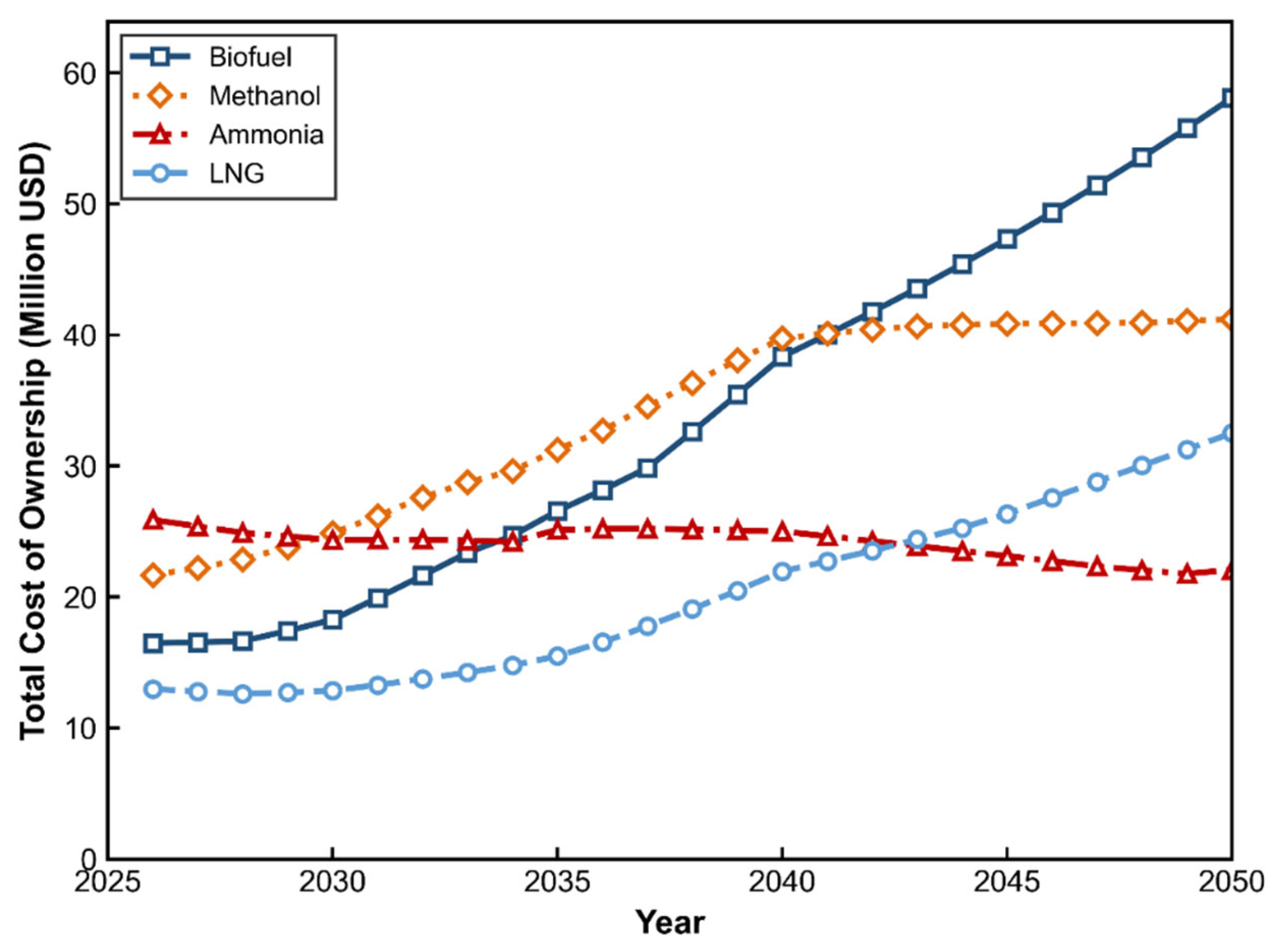
The evolution of the TCO trajectories reveals three distinct phases characterized by shifting cost-competitiveness (Figure 1). During the initial phase (2025–2030), conventional fuels retain a clear cost advantage. The biofuel pathway, operating mainly on fossil HFO with minor blending, maintains a TCO of approximately $16.5 million, exceeding the LNG pathway ($13.5 million) but remaining substantially lower than ammonia ($26.8 million). Between 2030 and 2040, regulatory tightening induces a rapid TCO surge for the biofuel route as expensive B100 substitution becomes mandatory. By 2035, the TCO of the ammonia pathway ($28.0 million) falls below that of biofuel. This critical cross-over point demonstrates that escalating compliance penalties ultimately outweigh the capital and operational costs of adopting zero-carbon propulsion. From 2040 to 2050, the biofuel pathway emerges as the most expensive option, reaching $60.0 million, indicating that an exclusive reliance on drop-in biofuels for legacy vessels is financially unsustainable relative to methanol or ammonia transitions, which stabilize at lower costs (approx. $22.5–$48.0 million).

4.1.2. Internal Fuel Substitution Strategy

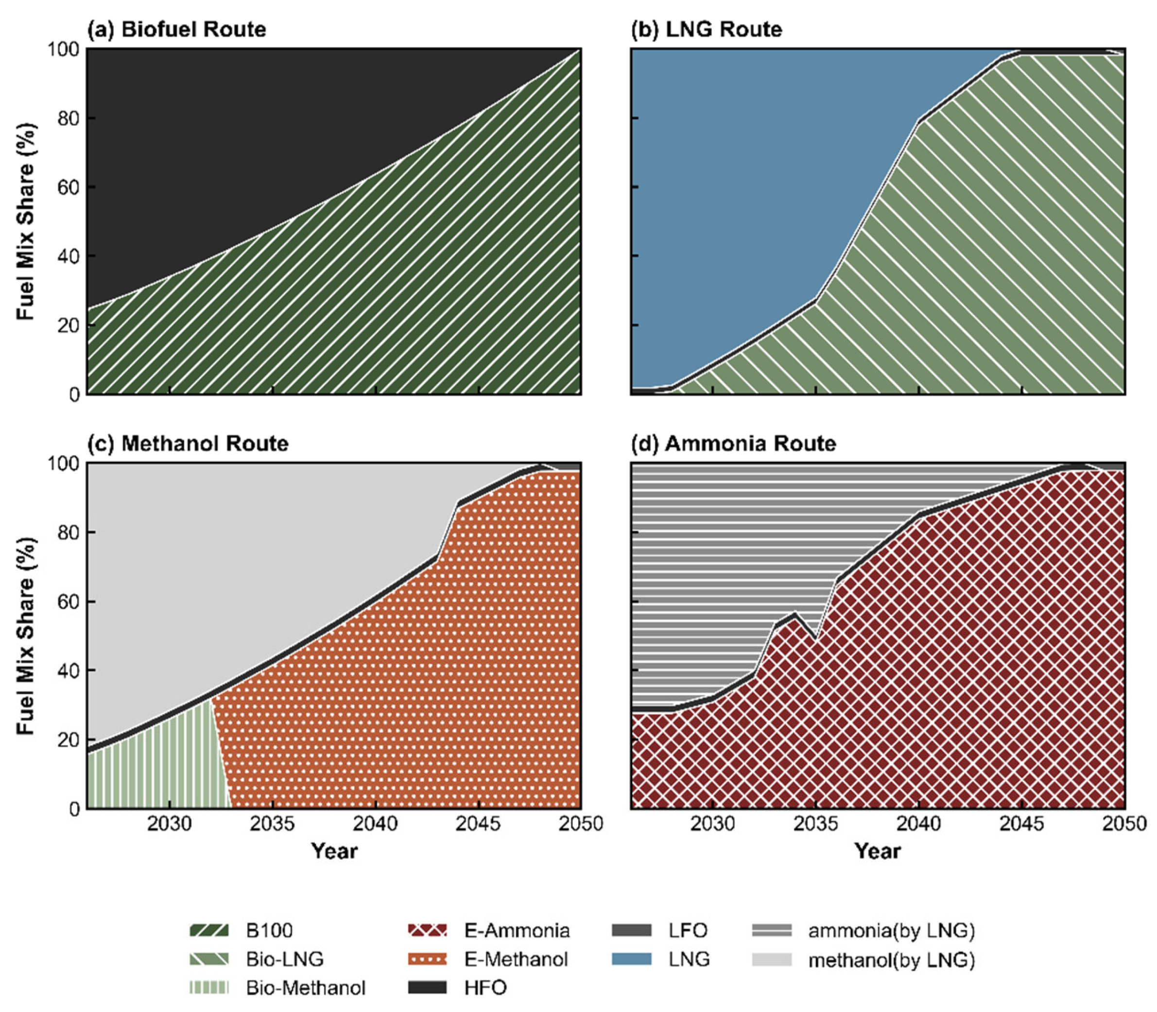
The intra-pathway fuel substitution dynamics are illustrated as 100% relative market shares in Figure 2, revealing distinct structural shifts driven by tightening GHG constraints.

In the biofuel pathway, the drop-in strategy initially relies on blending B100 with conventional HFO (Figure 2a). B100 accounts for approximately 25% of the fuel mix by 2026 and continues to expand under increasing regulatory pressure. A critical tipping point is reached around 2040, where B100 crosses the 60% threshold, decisively surpassing HFO and culminating in full substitution (100%) by 2050. The resulting cost escalation is associated with complete dependence on high-cost premium biofuels under fixed engine configurations.

In the LNG pathway, fossil LNG maintains near-total dominance until the late 2020s (Figure 2b). Bio-LNG is introduced incrementally, capturing approximately 30% of the mix by 2035, before expanding rapidly to achieve full substitution (100%) just after 2045. This delayed transition maintains cost stability in the medium term while introducing long-term exposure to bio-LNG supply constraints.

The methanol pathway exhibits a distinct multi-stage transition (Figure 2c). Gray methanol (methanol by LNG) dominates the early period, supplemented by a bio-methanol blend that scales from approximately 20% to 35% by 2033. Crucially, e-methanol enters abruptly thereafter, entirely displacing bio-methanol and expanding to fully replace gray methanol (100%) by 2050. This structural shift confirms a reliance on large-scale Power-to-X deployment for long-term compliance rather than limited biomass-based supply.

In the ammonia pathway, low-carbon adoption occurs earlier and more aggressively than in other pathways (Figure 2d). E-ammonia captures approximately 28% of the mix in 2026 and exhibits steady growth, decisively overtaking gray ammonia by 2040 (reaching approximately 78% share) and achieving exclusive substitution (100%) by 2050. This early and sustained deployment contributes to improved long-term cost positioning relative to the biofuel and LNG pathways.

4.2. Fleet Structure Dynamics and Technology Diffusion

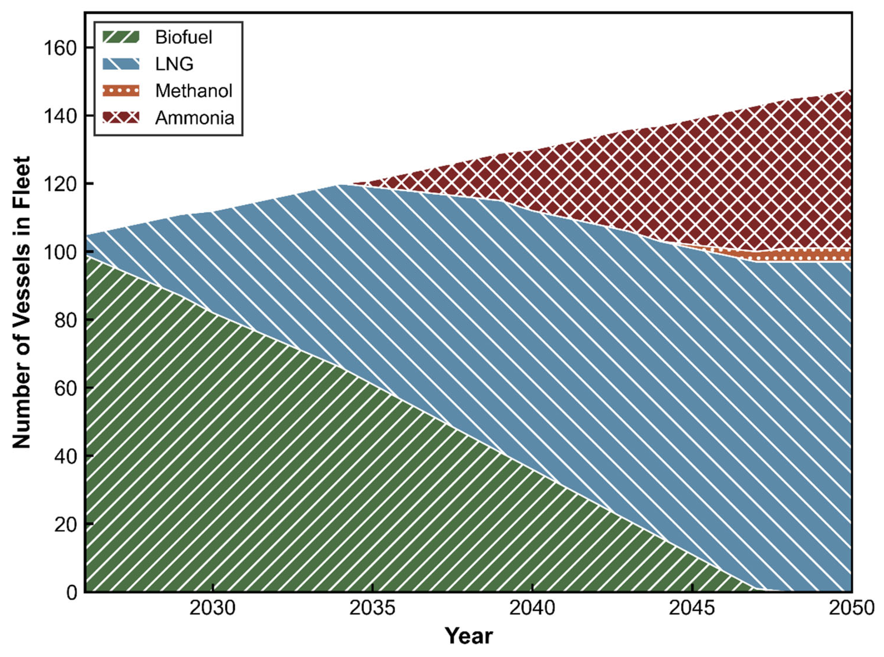
Figure 3 illustrates the evolution of the fleet’s fuel composition from 2025 to 2050 under the baseline scenario. The simulation reflects a baseline trajectory driven by TCO optimization, representing market selection absent external policy distortions.

The most prominent feature of fleet evolution is the dominance of Liquefied Natural Gas (LNG). Capturing the vast majority of the newbuilding market between 2026 and 2040, LNG provides the lowest fuel prices and most mature engine technology without additional carbon levies. It functions as the most cost-effective transitional solution for shipowners balancing fleet renewal with operational expenditures (OPEX).

Ammonia adoption is initially delayed by the economic disparity between fossil-based and zero-carbon fuels. However, as the fleet expands toward 2050, ammonia’s market share steadily increases, indicating improved long-term cost competitiveness capable of challenging incumbent LNG assets.

The conventional biofuel/oil fleet demonstrates a consistent decline, constrained by a global retrofit capacity limit of 5 vessels per year. This stable linear retirement trajectory confirms that decarbonization is structurally bounded by shipyard throughput and legacy asset lifecycles, phasing out completely by 2048.

Despite technical maturity, baseline results indicate marginal uptake of methanol-fueled vessels. Primitive market data projects significantly higher unit costs for green methanol relative to LNG and ammonia. In pure TCO optimization without corridor-specific subsidies, methanol is restricted to niche retrofit scenarios where CAPEX savings temporarily offset OPEX burdens, failing to achieve mainstream adoption.

4.3. Decarbonization Trajectory and Energy Demand Implications

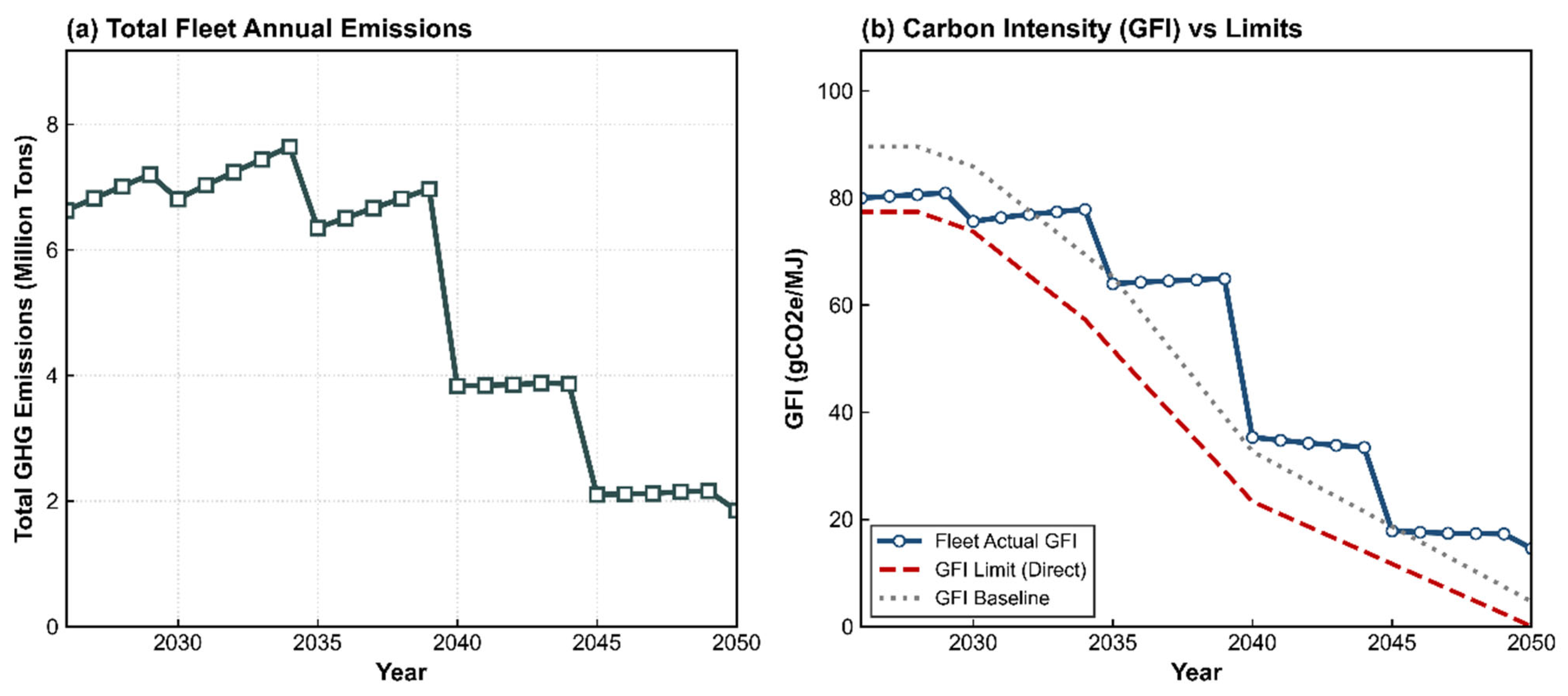
Under baseline conditions, the fleet follows a non-linear decarbonization trajectory (Figure 4a). Total annual GHG emissions increase from 6.5 million tons in 2025 to a peak of 7.6 million tons in 2035, despite early LNG adoption. The ~20% emission reduction associated with fossil LNG is insufficient to offset fleet expansion at approximately 3% per year. Emissions begin to decline after 2038 with the large-scale deployment of synthetic fuels, reaching approximately 1.9 million tons by 2050, equivalent to a 75% reduction from the peak. The inability to achieve absolute zero emissions is driven by both residual fossil LNG usage and the inherent upstream (Well-to-Tank) carbon footprint accounted for in the WTW lifecycle of synthetic alternatives.

The fleet-average GFI exhibits persistent compliance deficits relative to the strict Direct limit throughout the projection period (Figure 4b), deeply reflecting the two-tier penalty dynamics. In the initial phase (prior to 2033), the fleet’s actual GFI safely remains below the upper Base target but above the Direct limit. This indicates a deliberate strategy to absorb moderate Tier 1 penalties rather than undertaking premature, capital-intensive transitions. However, between 2033 and 2039, a pronounced compliance bottleneck emerges. As the Base target drops steeply, reliance on fossil LNG fails to keep pace, pushing the fleet GFI to temporarily breach the punitive Tier 2 threshold. While the large-scale expansion of zero-carbon synthetic fuels after 2040 triggers significant step-down reductions, the trajectory continually hovers above the Direct limit. Since the model boundary explicitly excludes financial rewards for over-compliance, generating surplus units offers no economic incentive to the solver. This behavior confirms a mathematically driven “marginal compliance” strategy: the fleet continually optimizes total expenditures by navigating tiered penalty thresholds, intentionally balancing the high costs of deep decarbonization against acceptable regulatory liabilities, strictly avoiding uncompensated emission reductions.

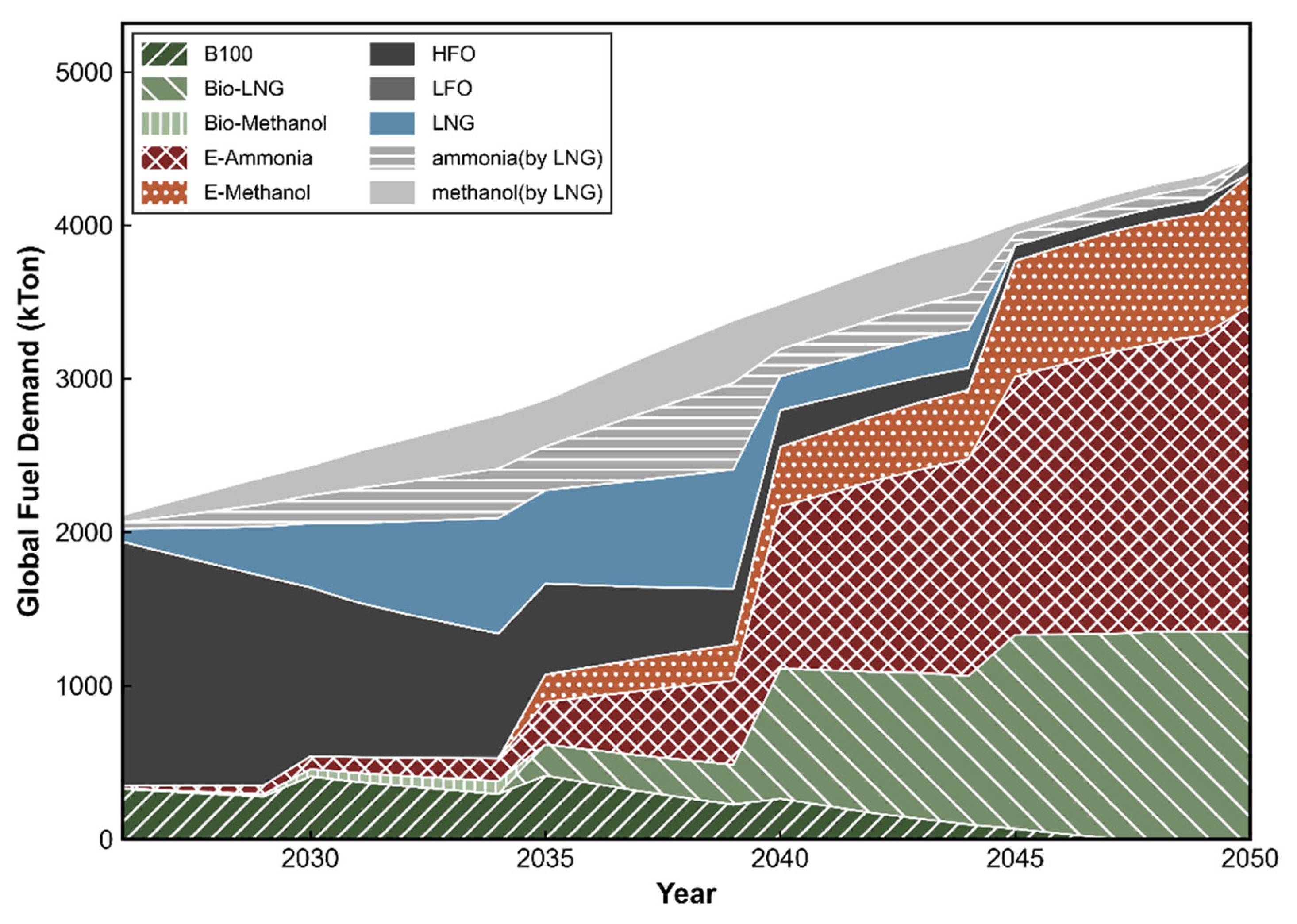
Aggregated fuel demand undergoes a structural shift from fossil-dominated consumption to synthetic and bio-derived fuels (Figure 5). In 2025, early compliance is achieved through 1698 kTon of conventional HFO blended with 351 kTon of B100. As fleet renewal progresses, both fuels decline steadily, dropping to a marginal ~5.7 kTon of B100 by 2047 before being fully phased out by 2048. This indicates that drop-in biofuels serve only as a transitional measure for legacy vessels rather than a scalable long-term solution.

Methanol and ammonia pathways exhibit complete substitution toward synthetic fuels. E-methanol expands after 2035 and fully replaces gray methanol by 2050, reaching 864 kTon. Ammonia follows a more rapid transition, with e-ammonia scaling to 2121 kTon by 2050 and becoming the dominant fuel category. This level of demand implies a substantial requirement for upstream renewable hydrogen supply to support electro-fuel production.

In the LNG pathway, initial reliance on fossil LNG shifts toward bio-LNG in the late stage to maintain compliance. Fossil LNG is eliminated by 2050, while bio-LNG demand reaches 1352 kTon. The absence of e-LNG adoption suggests that biomass-derived LNG retains a cost advantage over synthetic alternatives under baseline conditions.

4.4. Sensitivity Analysis

This section evaluates the robustness of the optimal pathway by examining how variations in regulatory penalty rates and fuel prices reshape the fleet’s decarbonization trajectory relative to the baseline scenario.

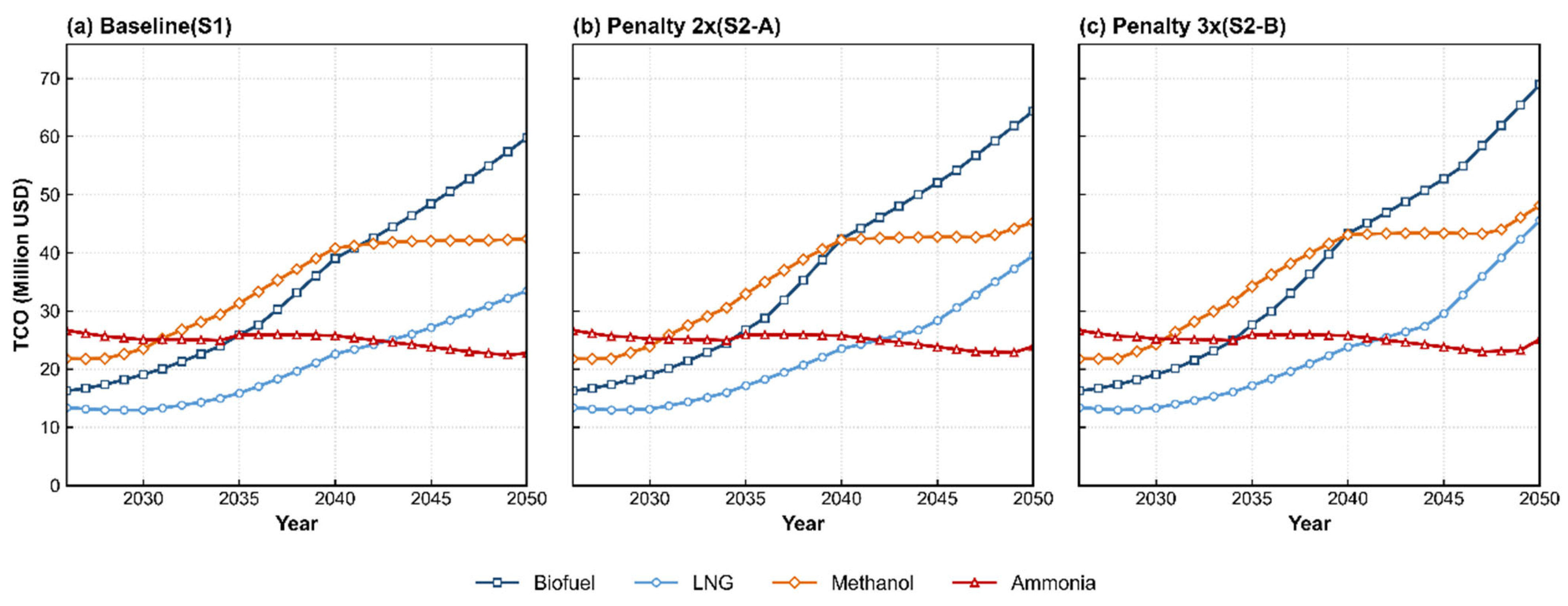
Under baseline conditions, fossil LNG remains the least-cost option for nearly two decades, with the TCO cross-over against zero-carbon ammonia occurring only around 2043 (Figure 6a). Contrary to the expectation of a dramatic shift, increasing penalty levels only marginally compresses this specific transition window. Even under a triple-penalty regime (Figure 6c), the LNG-ammonia cross-over only advances slightly to approximately 2041. This inertia indicates that LNG’s lower baseline emission profile effectively shields it from severe early-stage penalties, rendering multipliers ineffective until regulatory limits tighten decisively in the late 2030s.

Instead, the punitive regimes fundamentally disrupt the mid-term viability of other transition pathways. Under the 3× penalty scenario, cumulative carbon liabilities drive the TCO of both the methanol and biofuel pathways sharply upward, forcing them to intersect with the zero-carbon ammonia baseline much earlier—around 2032 and 2034, respectively. By 2050, the biofuel drop-in strategy becomes the most economically punitive option, approaching $70 million. Under these conditions, drop-in blending loses economic viability early on, and a direct leap to zero-carbon propulsion becomes necessary for high-carbon baseline pathways to avoid asset stranding.

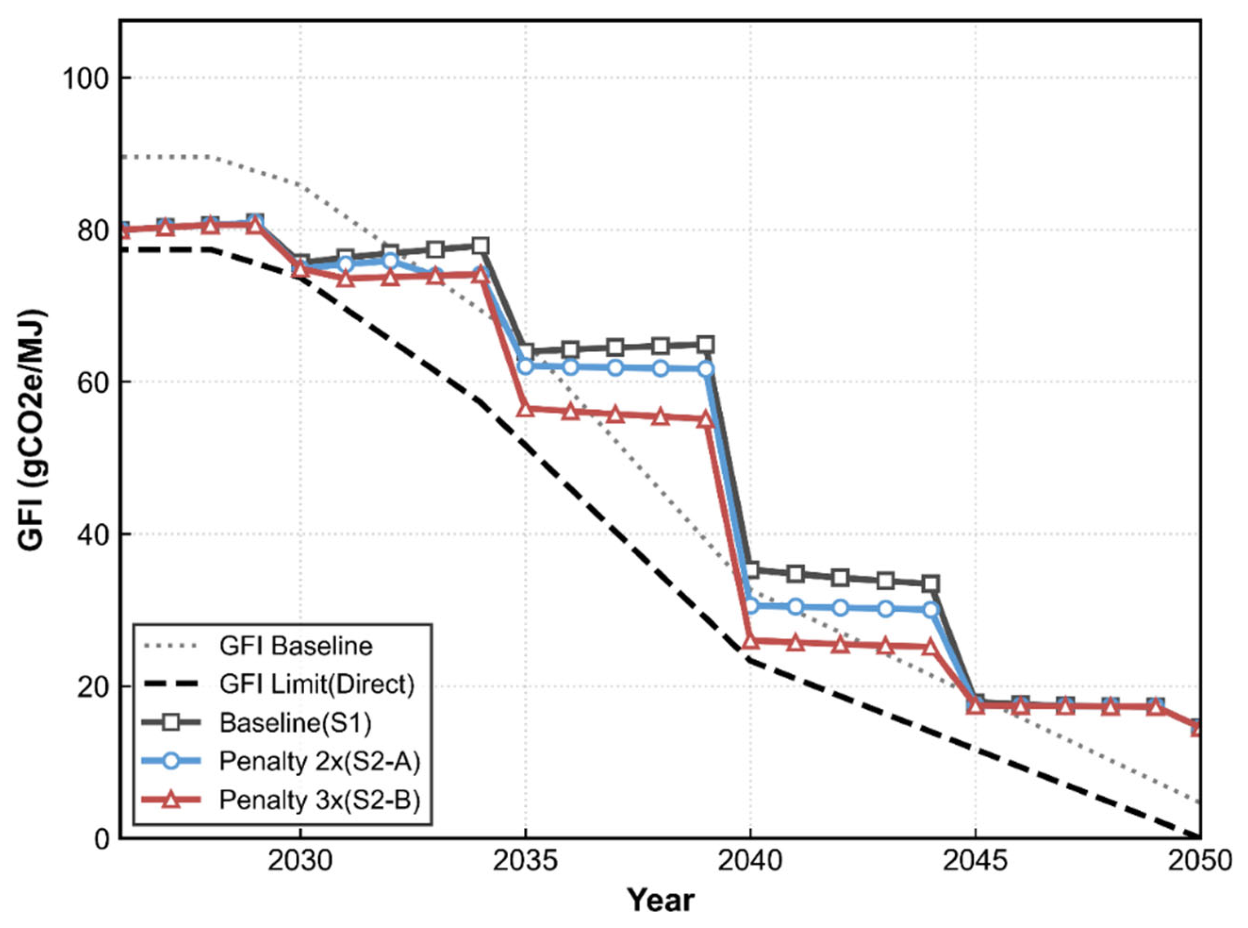
At the fleet level, the GFI trajectories across different scenarios (Figure 7) vividly illustrate the fleet’s strategic navigation of the two-tier penalty mechanism. In the baseline case, the fleet’s GFI deliberately breaches the upper Base target (gray dotted line) during the mid-2030s, reflecting a “pay-to-pollute” tolerance where standard Tier 2 penalties remain economically preferable to deep decarbonization. As penalty multipliers increase, the fleet dynamically shifts its strategy to evade amplified punitive costs. Under the strict 3× penalty regime (S2-B), the GFI trajectory is forced sharply downward in 2035 specifically to remain below the dropping Base target, entirely avoiding the severe Tier 2 zone. Crucially, across all scenarios, the trajectories strictly remain above the lower Direct limit (black dashed line). This confirms that while heavy penalties effectively compress the fleet into the intermediate Tier 1 penalty zone, they do not induce voluntary over-compliance, reinforcing the enduring resilience of the marginal compliance strategy.

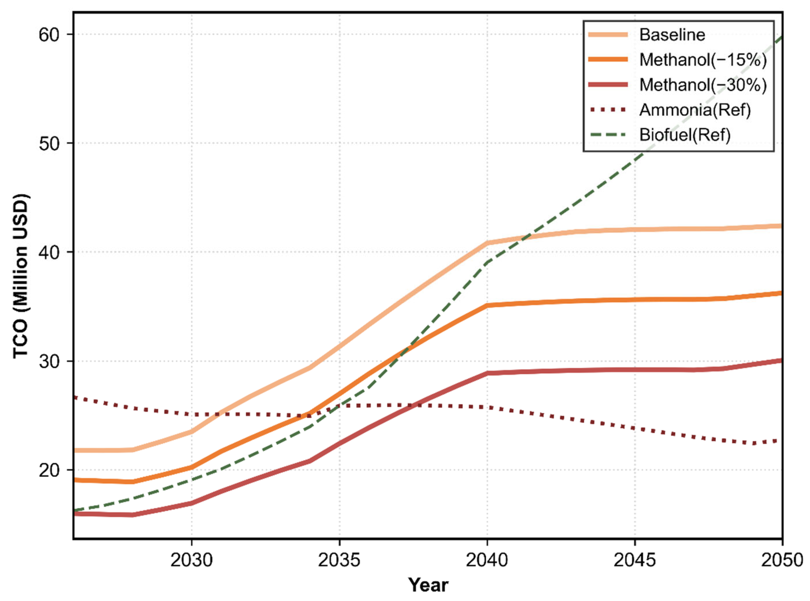
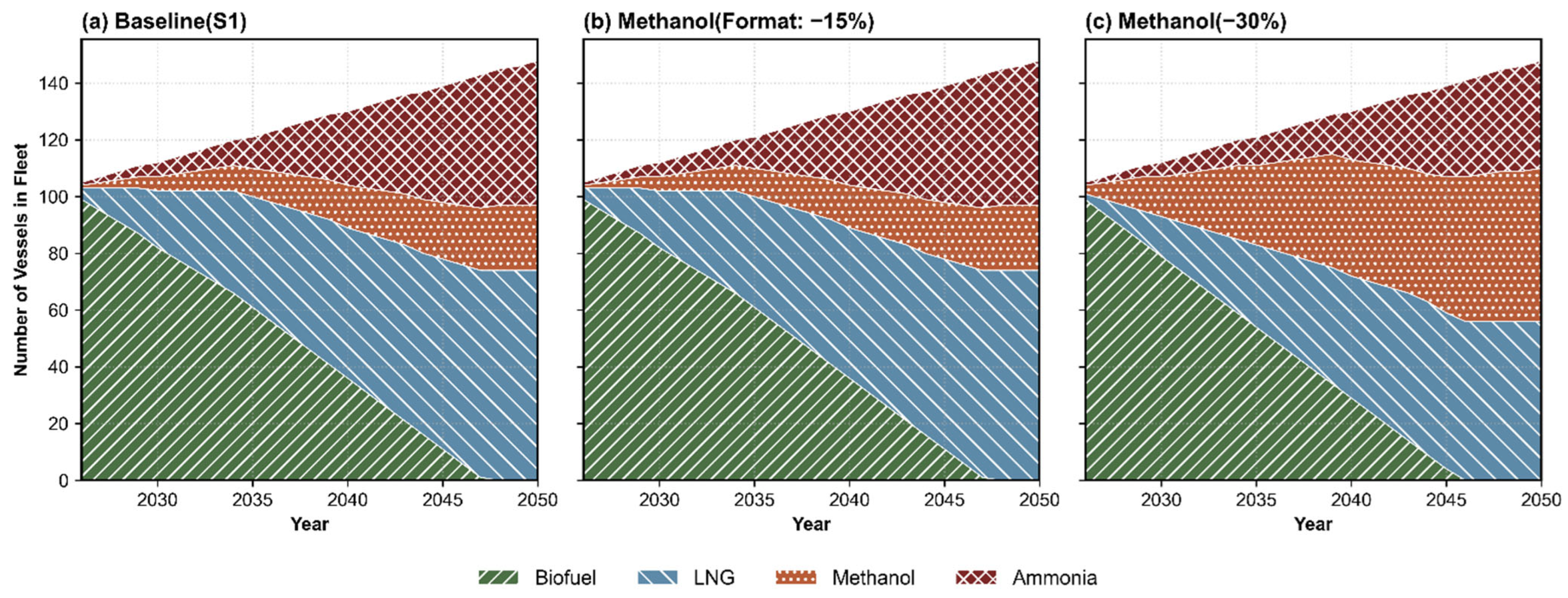
The role of economic incentives is illustrated through methanol price sensitivity. A 15% reduction in feedstock costs lowers methanol TCO but does not achieve parity with ammonia, remaining above the reference trajectory throughout the projection period and approaching the biofuel benchmark only around 2030 (Figure 8). A 30% reduction produces a structural shift: methanol intersects the biofuel pathway by 2028 and ammonia around 2038, becoming the most competitive low-carbon option in the mid-term. At the fleet scale, this cost shift expands methanol adoption, displacing part of LNG’s mid-term share and ammonia’s long-term dominance, resulting in a diversified three-fuel structure by 2050 (Figure 9).

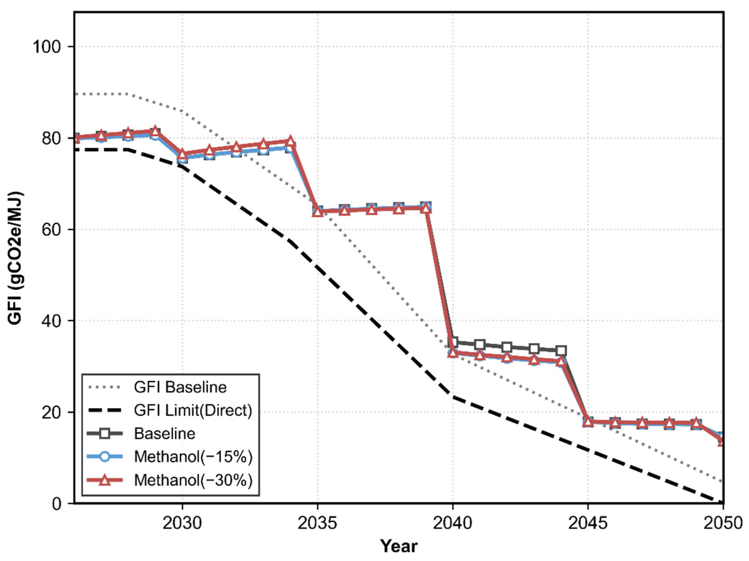
Despite these changes in fuel composition, the decarbonization trajectory remains largely unchanged. GFI compliance paths are nearly identical across scenarios (Figure 10), indicating that regulatory limits determine the pace of emission reduction, while relative fuel prices determine the technology mix. Methanol adoption therefore depends primarily on cost competitiveness, with a 30% feedstock reduction representing the threshold at which it becomes structurally relevant without altering overall emission outcomes.

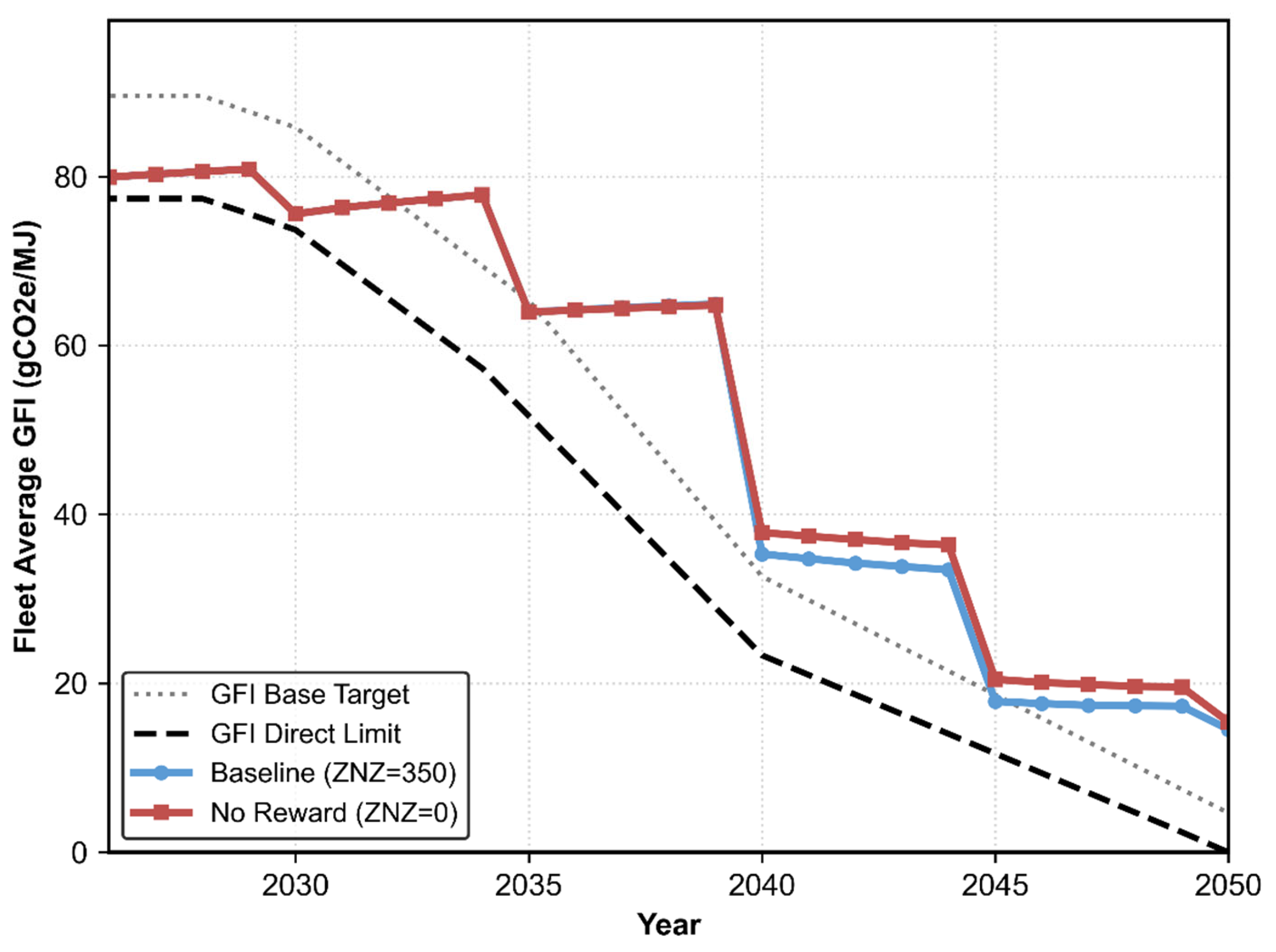
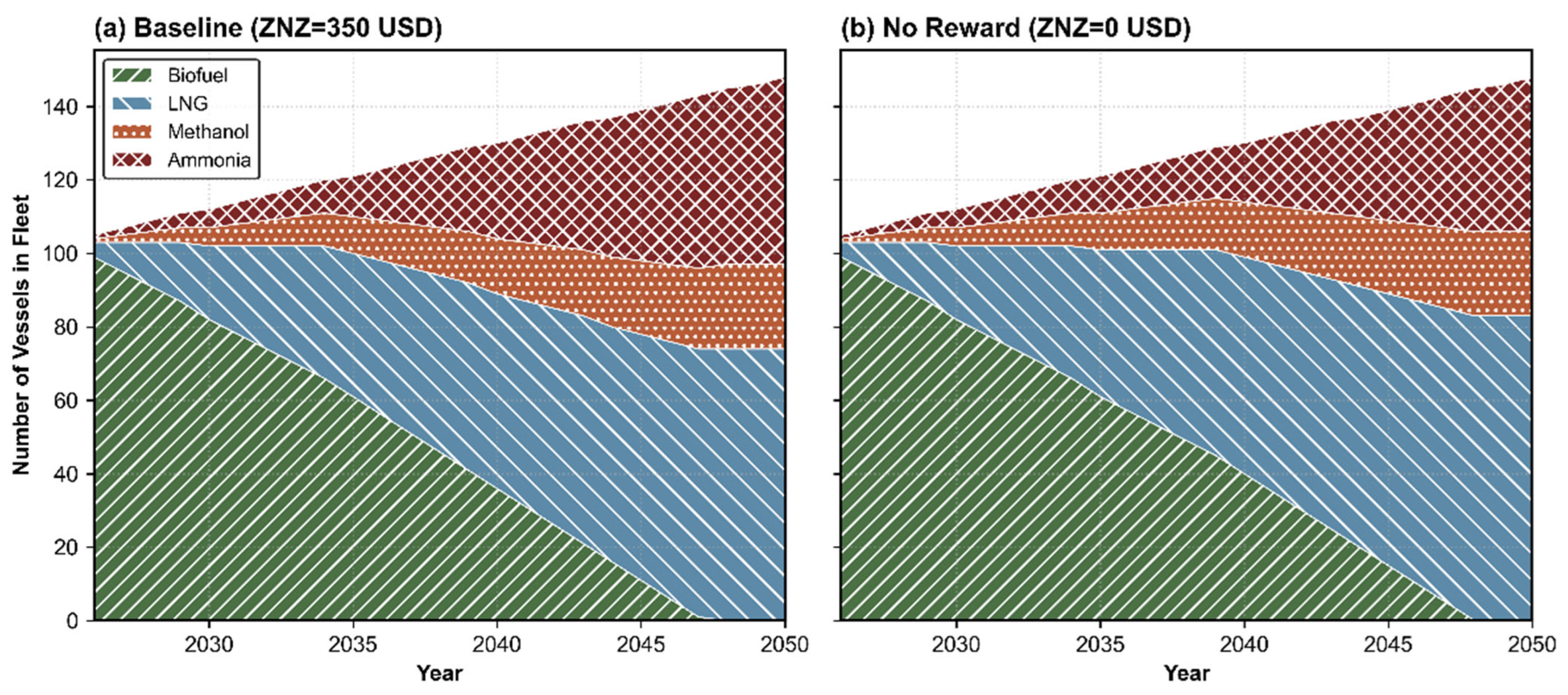
To address potential concerns regarding the model’s structural dependence on financial incentives, a counterfactual scenario excluding the ZNZ emissions reward (ZNZ = 0) was evaluated. As depicted in Figure 11 and Figure 12, removing the 350 USD/tCO₂e reward does not fundamentally reverse the overall transition direction toward low-carbon fuels, but it significantly delays the penetration of synthetic alternatives.

Figure 11 illustrates the comparative fleet mix evolution. It indicates that LNG serves as the primary interim compliance option in both scenarios. However, without the ZNZ reward to offset initial green premiums, the adoption window for e-methanol is noticeably compressed, and the large-scale transition to e-ammonia is postponed. Consequently, the fleet relies on fossil LNG for a prolonged duration, increasing the risk of mid-term technology lock-in.

Figure 12 further reveals the economic trade-offs in regulatory compliance. Under the IMO framework, exceeding the Direct Limit incurs Tier 1 penalties (100 USD/tCO₂e), while breaching the Base Target triggers severe Tier 2 penalties (380 USD/tCO₂e). While both trajectories exceed the Direct Limit throughout most of the 2030s, the unsubsidized trajectory (ZNZ = 0) exhibits a more persistent compliance deficit, pushing the fleet average GFI toward the Base Target. This demonstrates that without the ZNZ reward, shipowners are economically incentivized to absorb Tier 2 penalties rather than adopt capital-intensive zero-carbon propulsion systems during the early transition stage. After 2045, as regulatory carbon-intensity limits become increasingly stringent, the two trajectories gradually converge. The comparison indicates that the ZNZ reward primarily accelerates the timing of synthetic fuel adoption and reduces medium-term compliance deficits, while the broader transition trend remains governed by tightening carbon intensity constraints. The ZNZ reward therefore influences the transition pace more strongly than the ultimate decarbonization direction under progressively tightening GFS constraints.

5. Conclusions and Policy Implications

5.1. Main Conclusions

The techno-economic optimization of the green shipping corridor indicates that fleet decarbonization is governed by three interacting mechanisms rather than the isolated performance of individual fuels.

The timing of decarbonization is primarily penalty-driven. Under baseline conditions, the fleet exhibits a delayed emission peak in 2035 and a late transition to zero-carbon fuels, with the TCO crossover occurring around 2043. This reflects a persistent marginal compliance regime in which fleets optimize GFI against penalty thresholds rather than absolute emission targets. Increasing carbon penalties shifts this crossover point forward by more than a decade, fundamentally altering investment risk profiles.

Technology selection is strongly price-dependent and characterized by threshold behavior. The long-term fuel mix responds more to upstream production costs than to operational efficiency differentials. Under the projected baseline price trajectories assumed in this study, a feedstock cost reduction on the order of 30% is required for methanol to become competitive with ammonia, triggering a transition from a single-fuel dominance pattern to a diversified multi-fuel equilibrium.

The transition pathway is further constrained by structural factors. Pilot fuel requirements and WTW emissions impose a lower bound on achievable decarbonization, preventing absolute zero emissions. As a result, residual fossil fuel use persists as an economically rational compliance buffer, producing a long-tail effect in the transition trajectory.

5.2. Policy Implications

The results indicate that current regulatory and market conditions can sustain a prolonged pay-to-pollute equilibrium if penalty levels remain below the marginal abatement cost of low-carbon fuels. Effective decarbonization therefore depends on maintaining a dynamic alignment between carbon penalties and the evolving green fuel premium, ensuring that compliance costs consistently favor structural fuel switching over penalty payments.

Fuel market outcomes are highly sensitive to relative price signals, implying that technology-neutral economic instruments are critical for avoiding pathway lock-in. Mechanisms such as bilateral Contracts for Difference (CfDs), jointly supported by corridor stakeholders (e.g., port authorities, shippers, and fuel suppliers), can reduce early-stage cost uncertainty, support multiple fuel pathways, and limit systemic risks associated with reliance on a single hydrogen-derived fuel.

Investment decisions are exposed to substantial regulatory uncertainty. The observed sensitivity of transition timing to penalty stringency implies that conventional single-fuel assets face elevated stranding risk. Flexible propulsion configurations, including ammonia- or methanol-ready designs, provide a hedge against this uncertainty by preserving optionality under shifting cost and policy conditions.

5.3. Limitations and Future Research

The analysis adopts a simplified representation of fuel availability, assuming spatially unconstrained supply over time. This abstraction omits the geographic heterogeneity of bunkering infrastructure and upstream supply chains. Incorporating spatial–temporal constraints into the modeling framework would enable a more detailed assessment of transition bottlenecks and infrastructure requirements, particularly for large-scale deployment of electro-fuels. Additionally, the model operates under inelastic demand assumptions, omitting the potential impact of cost pass-through mechanisms and freight rate elasticity on long-term capacity expansion. In practice, significant increases in compliance costs may not be fully transferable to shippers, potentially affecting trade demand, routing decisions, and fleet deployment.