Data-Driven Technique for Fault Detection and Localization of Air Quality Process

Abstract

Air pollution is primarily caused by human activities such as industrial emissions, road traffic, waste incineration, and fossil fuel power plants. Pollution refers to the presence of harmful substances in the air, such as nitrogen dioxide (NO₂), sulfur dioxide (SO₂), ozone (O₃), carbon monoxide (CO), and other environmental pollutants. Some pollutants pose health risks even at low doses. Given the critical importance of air quality, monitoring air pollution has become an urgent and essential subject. Air quality monitoring relies on accurate data, so changeable environments and sensor issues make using interval diagnostic techniques for addressing uncertainty in systems interesting. In this article, we focus on three key aspects to achieve precise and efficient results: (1) the use of an accurate fault detection method that accounts for data uncertainty while maintaining model symmetry, (2) the implementation of a reliable detection index invariant to symmetric sensor behaviors, and (3) the combination of both to improve fault localization accuracy. This paper presented a fault detection and localization framework designed for uncertain and nonlinear monitoring environments. A novel fault-sensitive detection index was developed and integrated into an elimination-based localization strategy within a reduced-rank interval kernel PCA (RR-IKPCA) model. By exploiting information contained in modified residual subspaces and explicitly accounting for measurement uncertainty, the proposed approach enhances fault sensitivity while preserving robust localization capability, as validated on the AIRLOR air quality monitoring network.

1. Introduction

Continuous monitoring systems have become indispensable in modern environmental and industrial infrastructures, particularly with the rapid deployment of large-scale air quality monitoring. Over the past decades, diagnostic monitoring methodologies have evolved significantly, transitioning from model-based and analytical redundancy approaches toward advanced data-driven techniques [1,2,3]. Early methods relied heavily on first-principles models [4], which, although effective in well-defined systems, were often difficult to implement in complex and dynamic environments such as urban air quality networks. These networks commonly use low-cost IoT sensors, including electrochemical sensors for gases (e.g., CO, NO₂) and optical sensors for particulate matter (PM2.5, PM10).

With the increasing availability of real monitoring data, multivariate statistical approaches emerged as practical solutions for capturing correlations among variables and detecting abnormal system behavior [5,6]. These techniques have been successfully applied to real air quality monitoring datasets for identifying sensor faults, calibration issues, and data inconsistencies across monitoring stations [7]. Accurate detection and validation of measurement errors is a crucial first step in air quality network monitoring, as it allows deviations from normal operating conditions to be identified based on observed data patterns [8]. The second is fault isolation, where the goal is to pinpoint the specific sensor or subsystem responsible for the detected anomaly.

Various successful statistical fault detection methods are developed in the literature to detect faults or anomalous changes in key measured air quality variables [9,10]; this task of fault detection is very important but remains limited to testing the presence of faults [11,12]. To identify defect variables, several Principal Component Analysis (PCA)-based techniques have been developed in the literature, like the defect localization procedure using residue structuring [10,13]. The principle is to construct a set of residues, so that each residue is responsive to certain defects and not to others.

However, the nonlinear and non-Gaussian nature of air quality data has motivated the development of more sophisticated approaches, including kernel PCA (KPCA) and its variants, which provide improved representation of complex relationships. In [14,15,16,17] the authors proposed an extension for fault isolation using kernel PCA techniques (KPCA) to deal with nonlinearity.

Recent research has increasingly focused on applying these techniques to real-world monitoring networks, integrating methods such as reduced-rank models [18,19] to solve the problem of large datasets by downsizing the kernel matrix. These monitoring techniques have produced good detection and localization results but only with certain systems. However, in industrial environments, sensor measurements are often affected by imprecision [20,21]. To address this uncertainty in fault detection, numerous studies have been conducted [22,23], leading to the development of several linear Interval Principal Component Analysis (IPCA) approaches documented in the literature. In [24], an MRPCA-based EWMA scheme is proposed for sensor fault detection in air quality monitoring networks. The approach is validated through simulation studies, showing that MRPCA, as a robust interval multivariate statistical method, effectively addresses model uncertainties and improves fault detection capability.

For nonlinear scenarios, the interval kernel PCA (IKPCA) method was introduced by the authors in [25,26]. Furthermore, when dealing with interval-valued data, only a limited number of recent dimensionality reduction techniques based on IKPCA have been proposed, including reduced IKPCA (RIKPCA) [27], reduced-rank IKPCA (RRIKPCA) [28], and interval reduced-rank KPCA using the kernel generalized likelihood ratio test (IRR-KGLRT) [29]. In addition, some of these techniques have been applied to interval-based fault isolation; however, only limited research has addressed fault location in uncertain conditions. For example, the authors in [26,30] proposed a linear fault localization approach based on interval PCA using the ISPE index. Also, a localization method based on adaptive CIPCA was proposed in [13].

In addition to the importance of properly selecting the method used for fault detection, the choice of the fault detection index is also crucial. In most studies, Hotelling’s T² and the SPE are the main indices used [11]; the former is defined in the principal subspace where eigenvalues dominant, making it difficult to detect defects [31]. The latter, Squared Prediction Error (SPE), is calculated in the residual subspace where it is more sensitive to errors, but existing work shows that this is not always the case; this index fails in some cases to give better detection, hence the idea in [32] to improve this statistic by exploiting modified residual subspaces. The proposed index captures fault-related variations that may remain undetected by classical Hotelling’s T² and SPE statistics and demonstrates good detection performance. The aim of this study is to apply this index to the diagnosis of air quality monitoring network data.

To locate or identify a defect is defined as the capability of the monitoring process to determine the location of the defect [3,33,34]. The proposed RRIKPCA-based fault detection and localization framework demonstrates strong performance in uncertain and nonlinear monitoring environments, as validated on the AIRLOR air quality monitoring network. AIRLOR, located in Lorraine, France, comprises twenty monitoring stations distributed across rural, peri-urban, and urban sites. Each station measures key air pollutants, including NO, NO₂, O₃, CO, and SO₂, while six stations also record additional meteorological parameters. The primary focus of this study is the detection of sensor faults measuring ozone (O₃) and nitrogen oxides (NO and NO₂). The observation vector contains 18 controlled variables, corresponding to the concentrations of O₃, NO, and NO₂ at each station. A total of 400 observations were used for training the reference model, and 1000 observations were used as testing data to evaluate the framework’s performance.

The proposed framework considers several sources of uncertainty commonly encountered in air quality monitoring systems, including meteorological variability and external environmental disturbances, sensor-related effects such as measurement noise and sensor drift due to aging, and calibration inaccuracies. By incorporating these uncertainty sources through interval modeling, the framework provides a more realistic representation of operating conditions and enhances the robustness of the monitoring process. In addition, the integration of interval modeling with the fault-sensitive detection index [D] improves the capability of identifying incipient sensor faults under highly non-stationary air quality data characterized by temporal variability and abrupt changes caused by meteorological conditions or local emission events. Unlike conventional residual-based indicators, which may fail to detect subtle deviations in such environments, the proposed index [D] effectively captures anomalies in the modified residual subspace while remaining robust to normal data fluctuations, thereby improving the reliability and timeliness of fault detection.

The elimination-based localization strategy further strengthens the approach by directly evaluating the impact of removing each variable on the detection index. Compared with reconstruction-based contribution (RBC) methods and contribution plots, which may suffer from smearing effects and ambiguous interpretations, the elimination principle provides clearer fault attribution.

Nevertheless, the proposed method has some limitations. It assumes the presence of a single dominant fault, which may reduce localization accuracy in multi-fault scenarios. In addition, the performance of the RRIKPCA model depends on the availability of representative fault-free training data.

This paper is planned as follows. In Section 2, a summary of interval kernel methods is presented in the first part, while the second part presents the mathematical formulation of the novel index [D]. In Section 3, we present the suggested RR-IKPCA localization method. Section 4 demonstrates the efficiency of the proposed fault detection and isolation method using a real air quality monitoring network data.

2. Interval Fault Detection Methods

For large majority of cases we cannot measure the true value. This impreciseness is caused by the uncertainties $\Delta \mathsf{{\rm Y}}$. We must take into consideration this uncertainty of the measured data ${\mathsf{{\rm Y}}}_j(k)$ that is composed of ${\underset{¯}{\mathsf{{\rm Y}}}}_j(k)$ and ${\overline{\mathsf{{\rm Y}}}}_j(k)$ is an effect of the incertitude of measurement [26,30]:

$$\left[{\mathsf{{\rm Y}}}_{\iota }(\kappa )\right]=\left[{\underset{¯}{\mathsf{{\rm Y}}}}_{\iota }(\kappa ),{\overline{\mathsf{{\rm Y}}}}_{\iota }(\kappa )\right],$$

(1)

and we define ${\underset{¯}{\mathsf{{\rm Y}}}}_j(k)={\mathsf{{\rm Y}}}_j(k)-\Delta \mathsf{{\rm Y}}$ as the lower bound and ${\overline{\mathsf{{\rm Y}}}}_j(k)={\mathsf{{\rm Y}}}_j(k)+\Delta \mathsf{{\rm Y}}$ as the upper bound.

$\left[X\right]$ is the form interval of the data matrix $X\in R^{N\times M}$ that contains the N sample of the M process sensors. $\left[X\right]$ is organized as follows:

$$\begin{array}{l}\left[X\right]=\left(\begin{array}{ccccc}\left[{\underset{¯}{\mathsf{{\rm Y}}}}_1\left(1\right),{\overline{\mathsf{{\rm Y}}}}_1\left(1\right)\right]\hfill & \cdots ·& \left[{\underset{¯}{\mathsf{{\rm Y}}}}_{\iota }\left(1\right),{\overline{\mathsf{{\rm Y}}}}_{\iota }\left(1\right)\right]& \cdots ·& \left[{\underset{¯}{\mathsf{{\rm Y}}}}_{\mathrm{M}}\left(1\right),{\overline{\mathsf{{\rm Y}}}}_M\left(1\right)\right]\\ ⋮\hfill & & ⋮\hfill & & ⋮\hfill \\ \left[{\underset{¯}{\mathsf{{\rm Y}}}}_1\left(\kappa \right),{\overline{\mathsf{{\rm Y}}}}_1\left(\kappa \right)\right]\hfill & & \left[{\underset{¯}{\mathsf{{\rm Y}}}}_{\iota }\left(\kappa \right),{\overline{\mathsf{{\rm Y}}}}_{\iota }\left(\kappa \right)\right]& & \left[{\underset{¯}{\mathsf{{\rm Y}}}}_{\mathrm{M}}\left(\kappa \right),{\overline{\mathsf{{\rm Y}}}}_M\left(\kappa \right)\right]\\ ⋮\hfill & & ⋮\hfill & & ⋮\hfill \\ \left[{\underset{¯}{\mathsf{{\rm Y}}}}_1\left(\mathrm{N}\right),{\overline{\mathsf{{\rm Y}}}}_1\left(\mathrm{N}\right)\right]\hfill & \cdots ·\hfill & \left[{\underset{¯}{\mathsf{{\rm Y}}}}_{\iota }\left(\mathrm{N}\right),{\overline{\mathsf{{\rm Y}}}}_{\iota }\left(\mathrm{N}\right)\right]\hfill & \cdots ·\hfill & \left[{\underset{¯}{\mathsf{{\rm Y}}}}_{\mathrm{M}}\left(\mathrm{N}\right),{\overline{\mathsf{{\rm Y}}}}_M\left(\mathrm{N}\right)\right]\hfill \end{array}\right)\hfill \\ \kappa =1,\dots ,\mathrm{N};\iota =1,\dots ,\mathrm{M}\end{array},$$

(2)

where N is the number of process variables and M is the number of observations of each process variable.

${\mathsf{{\rm Y}}}_{\iota }^c(\kappa )$ and ${\mathsf{{\rm Y}}}_{\iota }^r(\kappa )$ are assumed by

$${\mathsf{{\rm Y}}}_{\iota }^c\left(\kappa \right)={\displaystyle \frac{1}{2}}\left({\overline{\mathsf{{\rm Y}}}}_{\iota }\left(\kappa \right)+{\underset{¯}{\mathsf{{\rm Y}}}}_{\iota }\left(\kappa \right)\right),{\mathsf{{\rm Y}}}_{\iota }^r\left(\kappa \right)={\displaystyle \frac{1}{2}}\left({\overline{\mathsf{{\rm Y}}}}_{\iota }\left(\kappa \right)-{\underset{¯}{\mathsf{{\rm Y}}}}_{\iota }\left(\kappa \right)\right),$$

(3)

A new numerical data matrix can be improved as follows:

$$\left[{\mathsf{{\rm Y}}}_{\iota }(\kappa )\right]=\left[{\mathsf{{\rm Y}}}_{\iota }^c(\kappa )-{\mathsf{{\rm Y}}}_{\iota }^r(\kappa ),{\mathsf{{\rm Y}}}_{\iota }^c(\kappa )+{\mathsf{{\rm Y}}}_{\iota }^r(\kappa )\right],$$

(4)

$$Y_{CR}=\left[\begin{array}{cc}{Y}^C& Y^R\end{array}\right],$$

(5)

With $Y^C=\left[{\mathsf{{\rm Y}}}_1^c,{\mathsf{{\rm Y}}}_2^c,\dots ,{\mathsf{{\rm Y}}}_r^c\right]\in R^{r\times \mathrm{M}}$ and $Y^R=\left[{\mathsf{{\rm Y}}}_1^r,{\mathsf{{\rm Y}}}_2^r,\dots ,{\mathsf{{\rm Y}}}_{\mathrm{N}}^r\right]\in R^{r\times \mathrm{M}}$, the new data is ${\mathsf{{\rm Y}}}_{CR}=\left[\begin{array}{cc}{\mathsf{{\rm Y}}}^c& {\mathsf{{\rm Y}}}^r\end{array}\right]\in R^{2\mathrm{M}}$.

The average and the variance of $\left[Y_{\iota }\right]$ are calculated by

$$M(\left[Y_{\iota }\right]={\displaystyle \frac{1}{n}}{\displaystyle \sum _{\kappa =1}^n\frac{{\overline{\mathsf{{\rm Y}}}}_{\iota }(\kappa )+{\underset{¯}{\mathsf{{\rm Y}}}}_{\iota }(\kappa )}{2}},$$

(6)

$$VAR(\left[Y_{\iota }\right])=〈\left[Y_{\iota }\right],\left[Y_{\iota }\right]〉={\displaystyle \sum _{\kappa =1}^{\mathrm{N}}\frac{1}{3}}({{\underset{¯}{\mathsf{{\rm Y}}}}^2}_{\iota }(\kappa )+{\underset{¯}{\mathsf{{\rm Y}}}}_{\iota }(\kappa ){\overline{\mathsf{{\rm Y}}}}_{\iota }(\kappa )+{{\overline{\mathsf{{\rm Y}}}}^2}_{\iota }(\kappa )),$$

(7)

With the vector $\left[Y_{\iota }\right]$ as

$$\begin{array}{l}\left[Y_{\iota }\right]={\left[\begin{array}{ccccc}\left[{\mathsf{{\rm Y}}}_{\iota }\left(1\right)\right]& \cdots & \left[{\mathsf{{\rm Y}}}_{\iota }\left(\kappa \right)\right]& \cdots & \left[{\mathsf{{\rm Y}}}_{\iota }\left(\mathrm{N}\right)\right]\end{array}\right]}^T=\\ {\left(\left[{\underset{¯}{\mathsf{{\rm Y}}}}_{\iota }(1),{\overline{\mathsf{{\rm Y}}}}_{\iota }(1)\right],\left[{\underset{¯}{\mathsf{{\rm Y}}}}_{\iota }(2),{\overline{\mathsf{{\rm Y}}}}_{\iota }(2)\right],\dots ,\left[{\underset{¯}{\mathsf{{\rm Y}}}}_{\iota }(\mathrm{N}),{\overline{\mathsf{{\rm Y}}}}_{\iota }(\mathrm{N})\right]\right)}^T\end{array},$$

(8)

The standardization of $\left[Y_{\iota }(\kappa )\right]$ is:

$${\displaystyle \frac{\left[{\mathsf{{\rm Y}}}_{\iota }(\kappa )\right]-M(\left[Y_{\iota }(\kappa )\right])}{\sqrt{VAR(\left[Y_{\iota }(\kappa )\right])}}}=\left[{\displaystyle \frac{\left[{\underset{¯}{\mathsf{{\rm Y}}}}_{\iota }(\kappa )\right]-M(\left[Y_{\iota }(\kappa )\right])}{\sqrt{VAR(\left[Y_{\iota }(\kappa )\right])}}},{\displaystyle \frac{\left[{\overline{\mathsf{{\rm Y}}}}_{\iota }(\kappa )\right]-M(\left[Y_{\iota }(\kappa )\right])}{\sqrt{VAR(\left[Y_{\iota }(\kappa )\right])}}}\right],$$

(9)

2.1. Review of IKPCA Methods

• IKPCA based on interval midpoint–radii:

The authors in [21,25] suggested involving uncertainties in the KPCA approach by two models: a model based on LBs and UBs and a model centered on midpoints and radii. Recently the models have been improved in [27,29] exploiting two reduction methods.

Remember that the kernel matrix K is

$$K=\left[\begin{array}{ccc}{\mathsf{\Gamma }}_1^T{\mathsf{\Gamma }}_1& \dots & {\mathsf{\Gamma }}_1^T{\mathsf{\Gamma }}_{\mathrm{N}}\\ \begin{array}{l}.\\ .\end{array}& \dots & \begin{array}{l}.\\ .\end{array}\\ {\mathsf{\Gamma }}_{\mathrm{N}}^T{\mathsf{\Gamma }}_1& \dots & {\mathsf{\Gamma }}_{\mathrm{N}}^T{\mathsf{\Gamma }}_{\mathrm{N}}\end{array}\right],$$

(10)

$\mathsf{\Gamma }$ is a nonlinear projection function in the characteristic space $\mathrm{H}$ (feature space):

$$\mathrm{H},\mathsf{\Gamma }:{\mathsf{{\rm Y}}}_i\in R^m\to {\mathsf{\Gamma }}_i=\mathsf{\Gamma }({\mathsf{{\rm Y}}}_i)\in R^h$$

$\mathsf{\Gamma }$ is specified by this propriety:

$$\mathsf{\Gamma }{({\mathsf{{\rm Y}}}_{\iota })}^T\mathsf{\Gamma }({\mathsf{{\rm Y}}}_{{\iota }^{\prime }})=\mathrm{k}({\mathsf{{\rm Y}}}_{\iota },{\mathsf{{\rm Y}}}_{{\iota }^{\prime }}),$$

(11)

With k(.,.) as the kernel function, there are several kernel functions [35,36]. Among these functions we mainly cite the Gaussian kernel (radial basis function, RBF) that is used in this paper and defined as follows:

$$\mathrm{k}({\mathsf{{\rm Y}}}_{\iota },{\mathsf{{\rm Y}}}_{{\iota }^{\prime }})=\exp \left[{\displaystyle \frac{-{‖{\mathsf{{\rm Y}}}_{\iota }-{\mathsf{{\rm Y}}}_{{\iota }^{\prime }}‖}^2}{2{\sigma }^2}}\right],$$

(12)

where σ is the width of a Gaussian function which controls the flexibility of the kernel. A typical choice for σ is the average minimum distance (d) between two points in the training data set, i.e., ${\sigma }^2=c{\displaystyle \frac{1}{N}}{\displaystyle \sum _{i=1}^N{\min }_{j\ne i}}{d}^2(x_i,x_j)$, where c is a user-defined scaling parameter [19]. For the AIRLOR air quality monitoring dataset, ccc was selected in the range 0.5–1.0 based on preliminary experiments, balancing sensitivity to sensor faults with robustness to normal measurement variability.

The new form of kernel matrix $K_{CR}$ is given by

$$K_{CR}==\left[\begin{array}{ccc}\mathrm{k}({\mathsf{{\rm Y}}}_{CR,1},{\mathsf{{\rm Y}}}_{CR,1})& \dots & \mathrm{k}({\mathsf{{\rm Y}}}_{CR,1},{\mathsf{{\rm Y}}}_{CR,r})\\ \begin{array}{l}.\\ .\end{array}& \dots & \begin{array}{l}.\\ .\end{array}\\ \mathrm{k}({\mathsf{{\rm Y}}}_{CR,r},{\mathsf{{\rm Y}}}_{CR,1})& \dots & \mathrm{k}({\mathsf{{\rm Y}}}_{CR,r},{\mathsf{{\rm Y}}}_{CR,r})\end{array}\right],$$

(13)

Both the ‘midpoint–radii’ and ‘upper–lower’ representations are introduced as equivalent ways to describe interval uncertainty in sensor measurements. While the midpoint–radii form provides an intuitive interpretation of the central value and deviation, the upper–lower representation is used as the primary formulation in the subsequent development of the RR-IKPCA-based framework. This choice ensures consistency in the mathematical derivation and simplifies the implementation of uncertainty modeling throughout the fault detection and localization process.

• IKPCA upper–lower:

The $\underset{\_}{K}$ data is given by

$$\underset{\_}{K}=\left[\begin{array}{ccc}\mathrm{k}({\underset{¯}{\mathsf{{\rm Y}}}}_1,{\underset{¯}{\mathsf{{\rm Y}}}}_1)& \dots & \mathrm{k}({\underset{¯}{\mathsf{{\rm Y}}}}_1,{\underset{¯}{\mathsf{{\rm Y}}}}_N)\\ \begin{array}{l}.\\ .\end{array}& \dots & \begin{array}{l}.\\ .\end{array}\\ \mathrm{k}({\underset{¯}{\mathsf{{\rm Y}}}}_N,{\underset{¯}{\mathsf{{\rm Y}}}}_1)& \dots & \mathrm{k}({\underset{¯}{\mathsf{{\rm Y}}}}_N,{\underset{¯}{\mathsf{{\rm Y}}}}_N)\end{array}\right],$$

(14)

The kernel matrix for upper-bound data is represented by

$$\overline{K}=\left[\begin{array}{ccc}\mathrm{k}({\overline{\mathsf{{\rm Y}}}}_1,{\overline{\mathsf{{\rm Y}}}}_1)& \dots & \mathrm{k}({\overline{\mathsf{{\rm Y}}}}_1,{\overline{\mathsf{{\rm Y}}}}_N)\\ \begin{array}{l}.\\ .\end{array}& \dots & \begin{array}{l}.\\ .\end{array}\\ \mathrm{k}({\overline{\mathsf{{\rm Y}}}}_N,{\overline{\mathsf{{\rm Y}}}}_1)& \dots & \mathrm{k}({\overline{\mathsf{{\rm Y}}}}_N,{\overline{\mathsf{{\rm Y}}}}_N)\end{array}\right],$$

(15)

2.2. Review of RR-IKPCA Methods

Previous monitoring techniques have been illustrated for fault detection and isolation in air quality network data monitoring and have provided good detection and localization results [37]. However, the main disadvantage of these techniques is the computation time [11] to generate models, which increases with the number of system variables.

The core concept of the proposed RR-KPCA method is to remove dependencies among variables in the feature space while retaining a reduced but representative subset of the original dataset. Let

$$Y_r={\left[{\mathsf{{\rm Y}}}_1,\dots ,{\mathsf{{\rm Y}}}_i,\dots ,{\mathsf{{\rm Y}}}_r\right]}^T\in R^{r\times m}$$

denote the reduced dataset, where r is the number of retained observations. The RR-KPCA-based fault detection approach operates in two stages: offline model training and online fault detection. During the offline stage, a compact reference model is constructed to capture the system’s normal behavior. This involves selecting observations that provide linearly independent representations in the transformed feature space, ensuring that only informative and system-relevant data are retained [38].

In the online stage, the derived model is applied to actively monitor the system, enabling the detection of anomalies as they occur. The parameter r is determined dynamically based on the rank of the kernel matrix, such that $rang(K_r^t)=r$.

The rank of the updated kernel matrix is calculated, its value leading to two cases:

If $rang(K_r^t)=r$, the new observation is added to the reduced matrix. Otherwise, if $rang(K_r^t)<r$ no change is made and we bring back the kernel matrix to its previous state.

With

$$K_r^t=\left[\begin{array}{cc}{K}_r^{t-1}& k_{x_t}\\ k_{x_t}^T& \mathrm{k}(x_1,x_t)\end{array}\right]\in R^{r\times r}$$

We obtain the reduced data matrix $Y_r\in R^{r\times m}$ and construct the reduced core matrix, by keeping only r observations.

For example, the reduced $K_{CR}$, denoted as $K_{CR}^r$, becomes

$$K_{CR}^r=\left[\begin{array}{ccc}{\mathrm{k}}_r(x_{CR,1},x_{CR,1})& \dots & {\mathrm{k}}_r(x_{CR,1},x_{CR,r})\\ \begin{array}{l}.\\ .\end{array}& \dots & \begin{array}{l}.\\ .\end{array}\\ {\mathrm{k}}_r(x_{CR,r},x_{CR,1})& \dots & {\mathrm{k}}_r(x_{CR,r},x_{CR,r})\end{array}\right],$$

(16)

With

$${\mathrm{k}}_r(x_{CR,k})={({\mathrm{k}}_r(x_{CR,1},x_{CR,k}),\dots ,{\mathrm{k}}_r(x_{CR,N},x_{CR,k}))}^T$$

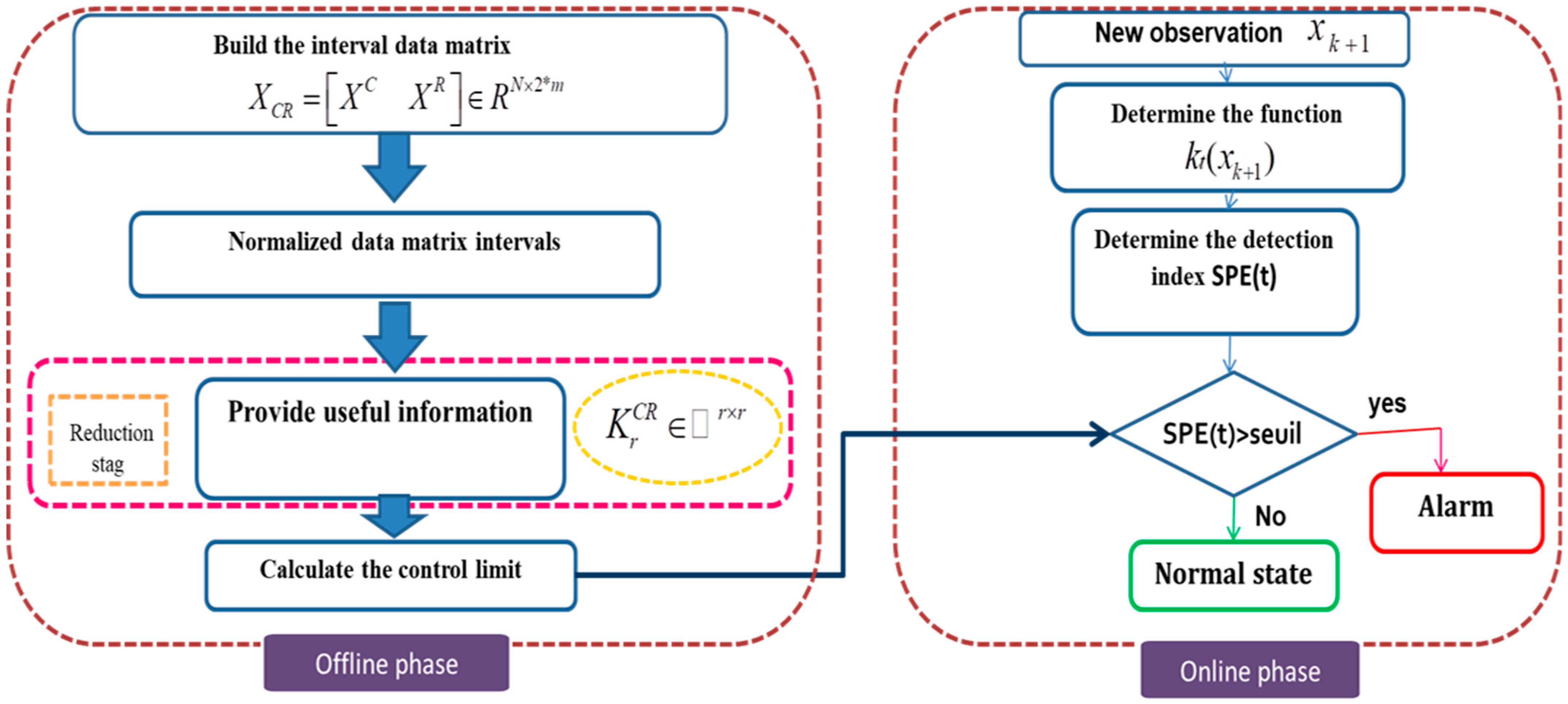
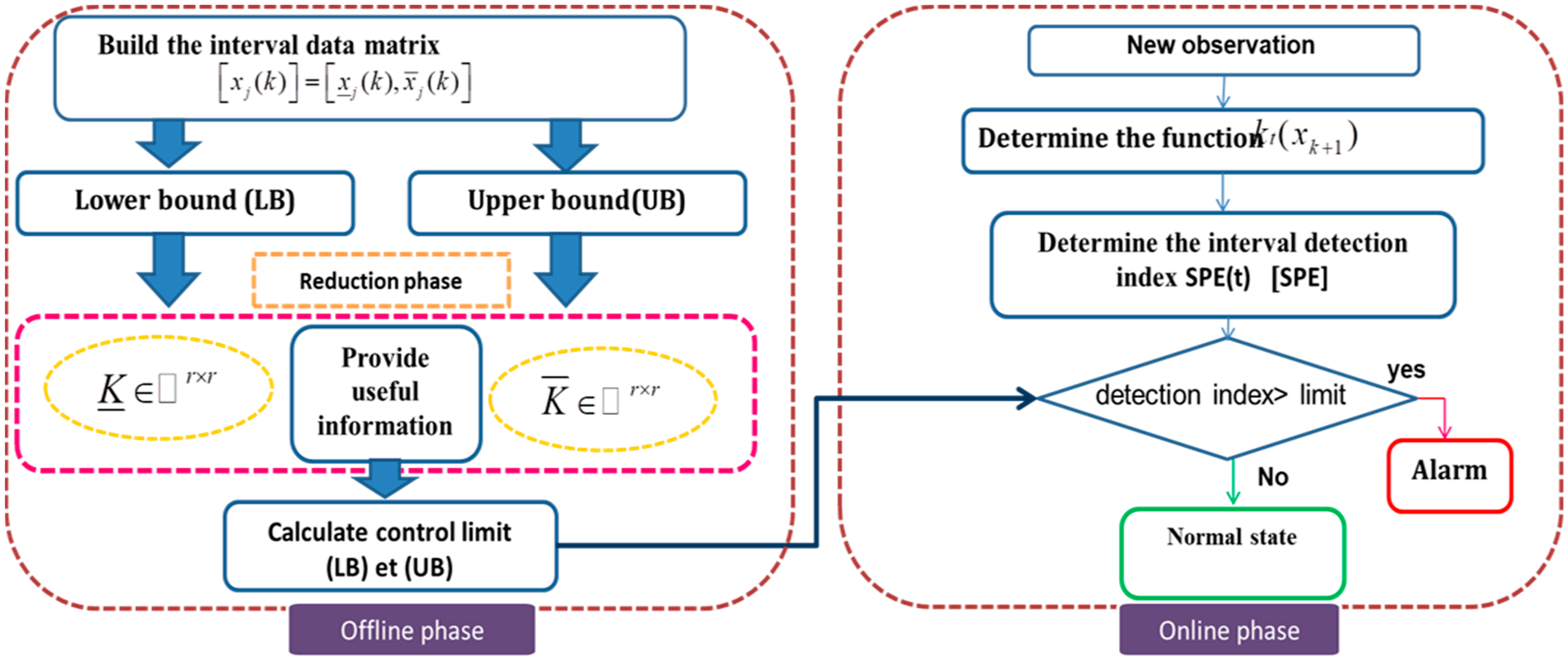
The reduction phase of RRIKPCA based on interval midpoint–radii is summarized in Figure 1 and the model based on upper and lower bounds in Figure 2.

2.3. Fault Detection Index

• The Center-Radius Approach Case

In classical PCA-based fault detection, the Squared Prediction Error (SPE) statistic is computed using the full residual subspace obtained after removing the dominant principal components. However, previous studies [39,40] have shown that important fault information may be contained in the least significant principal components, which are often neglected in conventional monitoring schemes.

To improve fault sensitivity for linear systems, ref. [32] proposed a detection index based on modified residual subspaces constructed by excluding a subset of dominant principal components and retaining only the last components associated with smaller eigenvalues. These components are more sensitive to incipient or low-energy faults, as they capture deviations that are not aligned with the main directions of normal process variability.

In this work, we extend this detection index to nonlinear systems by embedding it within an interval kernel PCA (IKPCA) framework. This extension preserves the sensitivity benefits of the least significant principal components while enabling the modeling of nonlinear process behavior and measurement uncertainty. The resulting index is subsequently used as the basis for fault detection and localization in the proposed methodology.

This index named Di corresponds to an SPE calculated with a PCA model with (m-i) principal components.

The parameter i is selected based on the variance contribution of the principal components and the residual analysis criterion. The proposed Di index detects abnormal deviations from the learned data correlation structure rather than high concentration values alone. Therefore, permanently high pollution levels measured near roads are treated as normal operating conditions when they are represented in the training data.

The expression of the new kernel center–range fault detection index is given by

$$D_{iCR}(k)={\mathrm{k}}_{CR}({\mathsf{{\rm Y}}}_{CR,k},{\mathsf{{\rm Y}}}_{CR,k})-{\mathrm{k}}^T({\mathsf{{\rm Y}}}_{CR,k}){\mathrm{V}}_{CR}\mathrm{k}({\mathsf{{\rm Y}}}_{CR,k}),$$

(17)

where $V_{CR}={\wp }_{CR}{\wp }_{CR}^T$.

$${\wp }_{CR}=\left[{\mathrm{B}}_{CR,1}^{-1}{\rho }_{CR,1}^T{\mathrm{A}}_{CR,1},\dots ,{\mathrm{B}}_{CR,\mathcal{l}}^{-1}{\rho }_{CR}^T{\mathrm{A}}_{CR,\mathrm{m}-\mathrm{i}}\right],$$

(18)

where ${\mathrm{A}}_{CR}$ and ${\mathrm{B}}_{CR}$ are the eigenvector and the eigenvalue of the reduced matrix $K_{CR}$ and ${\rho }_{CR}^T$ is the mapped data.

If $D_{iCR}(k)>{\tau }_{i,\alpha }^2$, a fault is detected, where ${\tau }_{i,\alpha }^2$ represent control limits.

The detection thresholds ${\tau }_{i,\alpha }^2$ [20] can be calculated by

$${\tau }_{i,\alpha }^2=g^{(i)}{\chi }_{h^{(i)},\alpha }^2,$$

(19)

• The Upper–Lower Approach Case

The interval form of $\left[D_i\right]$ index is represented as follows:

$${\underset{¯}{D}}_i(k)=\mathrm{k}({\underset{¯}{x}}_{r,k},{\underset{¯}{x}}_{r,k})-{\mathrm{k}}^T({\underset{¯}{x}}_{r,k}){\underset{¯}{V}}_r\mathrm{k}({\underset{¯}{x}}_{r,k}),$$

(20)

$${\overline{D}}_i(k)=\mathrm{k}({\overline{x}}_{r,k},{\overline{x}}_{r,k})-{\mathrm{k}}^T({\overline{x}}_{r,k}){\overline{V}}_r\mathrm{k}({\overline{x}}_{r,k}),$$

(21)

where

$$\begin{gathered} {\underset{¯}{V}}_r={\underset{¯}{\wp }}_r{\underset{¯}{\wp }}_r^T,{\underset{¯}{\wp }}_r=\left[{\underset{¯}{\mathrm{B}}}_{r,1}^{-1}{\underset{¯}{\rho }}_{r,1}^T{\underset{¯}{\mathrm{A}}}_{r,1},\dots ,{\underset{¯}{\mathrm{B}}}_{r,\mathcal{l}}^{-1}{\underset{¯}{\rho }}_r^T{\underset{¯}{\mathrm{A}}}_{r,\mathrm{m}-\mathcal{l}}\right], \\ {\overline{\wp }}_r=\left[{\overline{\mathrm{B}}}_{r,1}^{-1}{\overline{\rho }}_{r,1}^T{\overline{\mathrm{A}}}_{r,1},\dots ,{\overline{\mathrm{B}}}_{r,\mathcal{l}}^{-1}{\overline{\rho }}_r^T{\overline{\mathrm{A}}}_{r,\mathrm{m}-\mathcal{l}}\right] \end{gathered}$$

(22)

where ${\underset{¯}{\mathrm{A}}}_r$, ${\overline{\mathrm{A}}}_r$ and ${\underset{¯}{\mathrm{B}}}_r$, ${\overline{\mathrm{B}}}_r$ are respectively the vectors and the eigenvalues of the reduced $\underset{¯}{K^r}$ and ${\overline{K}}^r$.

3. Suggested Localization Method

3.1. Principle

The proposed localization method is based on the elimination principle, which is conceptually similar to the reconstruction-based contribution (RBC) approach [31,41]. Once a fault has been detected, the influence of each monitored variable on the detection index is assessed by successively removing one variable at a time from the monitoring model. This is achieved by modifying the PCA model through the elimination of the column corresponding to the excluded variable and computing the associated detection index. The relationship between the obtained index and its corresponding threshold is then evaluated through a diagnostic ratio. A significant reduction in this ratio indicates that the eliminated variable has a strong contribution to the detected fault and is therefore identified as the most likely faulty variable. Unlike classical RBC methods developed for deterministic linear PCA models, the proposed approach integrates interval-based fault detection, explicitly accounting for measurement uncertainty and nonlinear behavior, which makes it particularly suitable for fault localization in uncertain and complex monitoring environments.

Localization Method Steps:

Step 1: Initial Fault Detection Step 2: Generation of Sub-Models for Diagnosis: From the global model (which includes all process variables), an ensemble of m sub-models is generated; each sub-model is created by removing one variable j from the set of monitored variables. Step 3: Recalculation of the Detection Index for Each Sub-Model For each sub-model (after removing variable j), a new detection index is computed. Step 4: Calculation of the Diagnostic Ratio For each sub-model, a ratio is calculated between the new detection index and its corresponding threshold; this ratio reflects how much the detection index changes when variable j is removed. Step 5: Faulty Variable Identification Among all the computed ratios, the smallest one is identified; the variable associated with the minimum ratio is considered the faulty variable.

3.2. Mathematical Formulation

Stork et al. [42] proposed an approach for fault localization. The philosophy behind this method is similar to that of Dunia et al. [43].

The elimination approach is similar to the reconstruction approach [43]. A set of detection indices is generated by extracting at each instant a variable from the set of the variables to be monitored and by modifying the matrix representing the PCA model by elimination of the column corresponding to the eliminated variable. The relationship between the value indices at the instant of detection and their thresholds are calculated. The ratio calculated after eliminating a variable with a value less than 1 indicates that this variable is the wrong variable.

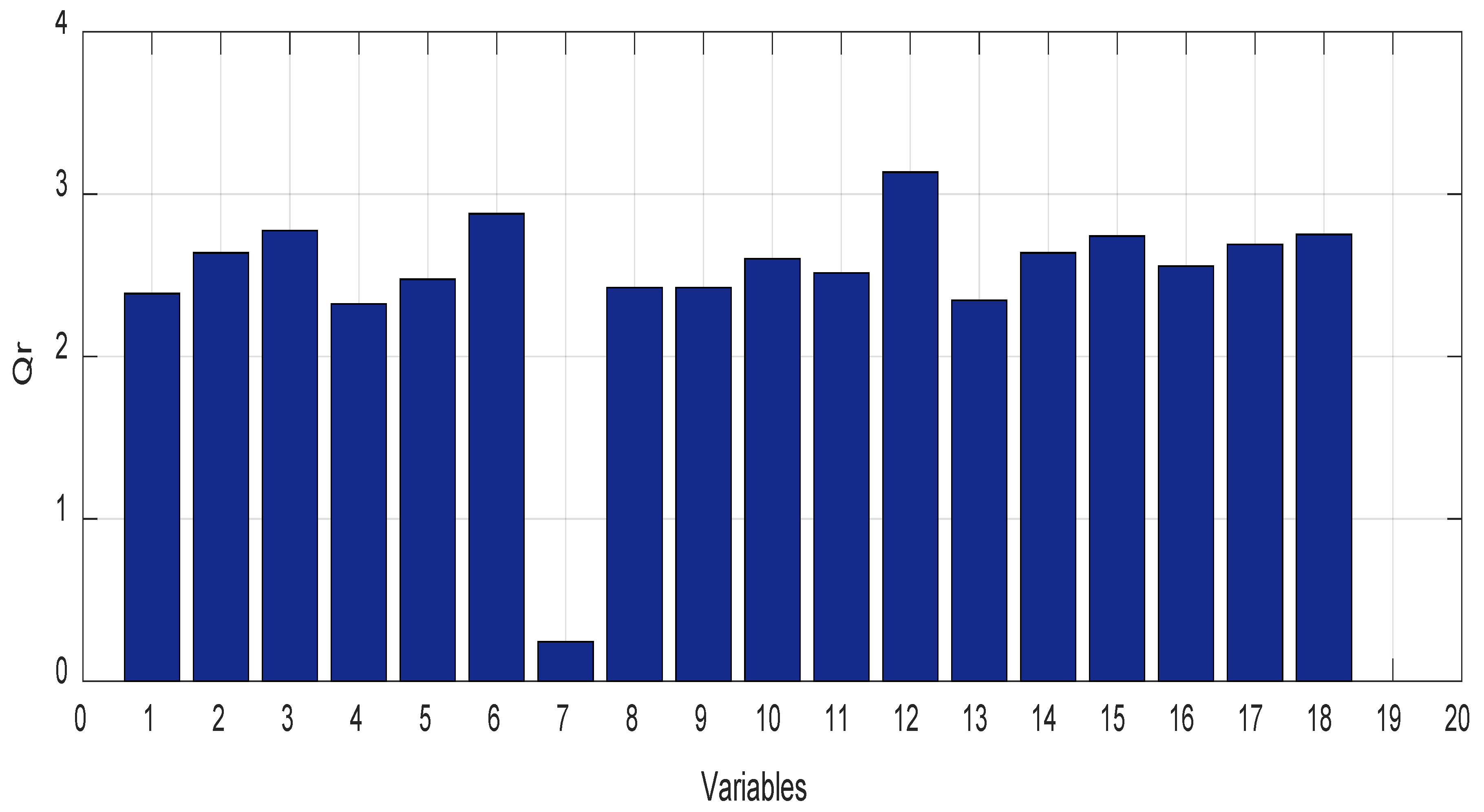
In the event that a fault is detected with the statistical $D_{{iCR}_{-j}}$, a set of PCA models is generated from the overall model by eliminating each time a variable from the set of variables to be monitored. The quantity is defined by $Q_r$ after the elimination of the jth variable. The defective variable is the jth variable, which corresponds to the smallest $Q_r$.

$$Q_{rCR}={\displaystyle \frac{D_{{iCR}_{-j}}}{Seui{l}_{D_{{iCR}_{-j}}}}},$$

(23)

With

$$D_{{iCR}_{-j}}(\mathrm{t})={\mathrm{k}}_{rCR}({\mathsf{{\rm Y}}}_{CR}^{-j},{\mathsf{{\rm Y}}}_{CR}^{-j})-{{\mathrm{k}}_{rCR}}^T({\mathsf{{\rm Y}}}_{CR}^{-j}){\wp }_{CR}{\wp }_{CR}^T{{\mathrm{k}}_{rCR}}^T({\mathsf{{\rm Y}}}_{CR}^{-j})$$

And the denominator is the corresponding detection threshold associated with the reduced model.

Q_rCR is calculated for each of the 18 reduced models, where each model is obtained by eliminating one variable at a time from the original monitoring model. The diagnostic ratio represents the normalized value of the detection index after variable elimination.

When a non-faulty variable is eliminated, the fault-related information remains in the reduced model, and the detection index stays close to or above its threshold, resulting in a ratio close to or greater than unity. In contrast, eliminating the faulty variable removes the primary source of abnormal variation from the model. This leads to a significant decrease in the detection index and, consequently, to a smaller diagnostic ratio.

Therefore, the variable associated with the minimum ratio corresponds to the variable whose removal most effectively suppresses the fault signature and is identified as the source of the fault.

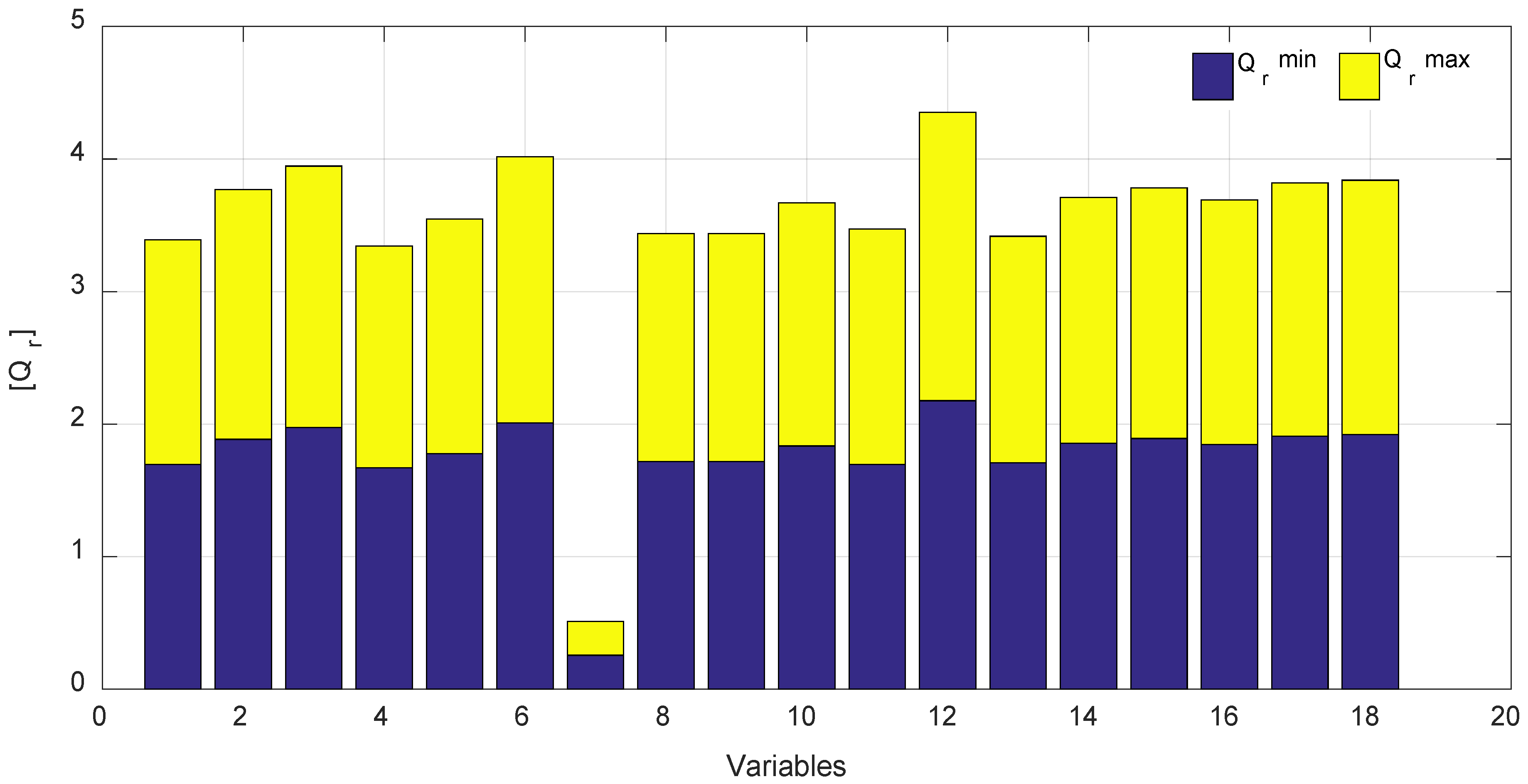
In the case of the upper- and lower-limit approach, the ratio is in its interval form with $\left[Q_r\right]=\left[{\underset{¯}{Q}}_r,{\overline{Q}}_r\right]$

$${\underset{¯}{Q}}_r={\displaystyle \frac{{\underset{¯}{D}}_{i_{-j}}}{Seui{l}_{{\underset{¯}{D}}_{i_{-j}}}}},{\overline{Q}}_r={\displaystyle \frac{{\overline{D}}_{i_{-j}}}{Seui{l}_{{\overline{D}}_{i_{-j}}}}},$$

(24)

$${\underset{¯}{D}}_{i_{-j}}(k)=\mathrm{k}({\underset{¯}{x}}_{r,k}^{-j},{\underset{¯}{x}}_{r,k}^{-j})-{\mathrm{k}}^T({\underset{¯}{x}}_{r,k}^{-j}){\underset{¯}{C}}_r\mathrm{k}({\underset{¯}{x}}_{r,k}^{-j}),$$

(25)

$${\overline{D}}_{i_{-j}}(k)=\mathrm{k}({\overline{x}}_{r,k}^{-j},{\overline{x}}_{r,k}^{-j})-{\mathrm{k}}^T({\overline{x}}_{r,k}^{-j}){\overline{C}}_r\mathrm{k}({\overline{x}}_{r,k}^{-j}),$$

(26)

In the proposed RR-KPCA-based fault detection framework, a diagnostic ratio value below 1 is used to indicate a potentially faulty variable. This threshold arises from the normalized formulation of the indicator, where values near 1 represent the boundary between nominal system behavior and statistically significant deviations from the learned reference model. In practical air quality monitoring systems, measurement noise and natural variability can cause short-term fluctuations around this threshold. Therefore, fault decisions are based not on a single instantaneous reading but on the temporal behavior of the indicator, such as repeated exceedances or persistent deviation below the threshold. This approach ensures that the diagnostic rule remains robust against transient noise while still effectively identifying genuinely faulty sensor measurements.

4. Application to the AIRLOR Air Quality Monitoring Network

AIRLOR Description

The air quality monitoring network AIRLOR, operating in Lorraine, France, is a comprehensive system that accumulates, examines, and validates air quality data across a wide geographical area. It plays a decisive role in ecological surveillance, sensor reliability, and supporting both research and policymaking in air quality management [8]. The details of this application are resumed in

Table 1. Description of air quality monitoring network AIRLOR.

Category	Details
Number of Stations	20
Station Locations	Rural, peri-rural, urban
Pollutants Monitored	NO, NO2, O3, CO, SO2
Stations with Meteorological Data	6 stations
Primary Objective	Detect sensor faults measuring O3, NO, and NO2 concentrations
Observation Vector	18 controlled variables (O3, NO, NO2 concentrations at each station) $x(k)={\left[\begin{array}{ccccc}\underset{O_3(k)\mathrm{NO}(k){\mathrm{NO}}_2(k):\mathrm{station}1}{\underbrace{v_1(k)v_2(k)v_3(k)}}& \dots & \underset{O_3(k)\mathrm{NO}(k){\mathrm{NO}}_2(k):\mathrm{station}4}{\underbrace{v_{10}(k)v_{11}(k)v_{12}(k)}}& \dots & \underset{O_3(k)\mathrm{NO}(k){\mathrm{NO}}_2(k):\mathrm{station}6}{\underbrace{v_{16}(k)v_{17}(k)v_{18}(k)}}\end{array}\right]}^T$
Training Data	400 observations
Testing Data	1000 observations
Uncertainty Introduced	2% of the range of each variable (added to data for robustness testing)
Fault Simulation	4 types of faults (described in Table 2; used to test the effectiveness of the proposed RR-IKPCA method)
Model Used	RR-IKPCA (reference model constructed using training data)

.

Although the AIRLOR monitoring network consists of 20 stations measuring several atmospheric pollutants, the observation vector used in this study was limited to 18 variables corresponding to synchronized measurements of O₃, NO, and NO₂ collected from a selected subset of monitoring stations. The selection was based on data completeness and temporal consistency over the analyzed period. Stations containing missing measurements, inconsistent sampling intervals, or incomplete historical records were excluded to ensure the reliability and consistency of the RR-IKPCA model training process. Consequently, the retained variables represent the subset of measurements providing stable multivariate correlations suitable for fault detection analysis.

Only six AIRLOR stations provide additional meteorological measurements. In the proposed framework, meteorological effects are not explicitly introduced as independent model inputs for all stations; instead, their influence is indirectly reflected through the correlation structure learned from the multivariate pollutant measurements. Furthermore, environmental deployment characteristics such as sensor height above ground level and proximity to emission sources may influence pollutant variability and inter-variable correlations. These spatial metadata were not explicitly incorporated into the present model and therefore constitute a limitation of the current study. Accordingly, the introduced 2% uncertainty should be interpreted as an assumed measurement uncertainty level used for robustness evaluation rather than a complete representation of all environmental and deployment-related variability.

Table 2. Different faults.

Faults	Additive Defect	Station	Observations
Fault 1	20% of the ordinary variation of (NO)	Station 1	Between 400 and 600
Fault 2	30% of the ordinary variation of (NO)	Station 1	Between 400 and 700
Fault 3	20% of the ordinary variation of (NO2)	Station 4	Between 300 and 600
Fault 4	40% of the ordinary variation of (O3)	Station 6	Between 400 and 600

Table 2. Different faults.

Faults	Additive Defect	Station	Observations
Fault 1	20% of the ordinary variation of (NO)	Station 1	Between 400 and 600
Fault 2	30% of the ordinary variation of (NO)	Station 1	Between 400 and 700
Fault 3	20% of the ordinary variation of (NO2)	Station 4	Between 300 and 600
Fault 4	40% of the ordinary variation of (O3)	Station 6	Between 400 and 600

5. Discussion

5.1. Results and Discussion

This section evaluates the fault detection performance of four RR-IKPCA-based monitoring strategies—RRIKPCA_UL using SPE and [D₄], and RRIKPCA_CR using SPE and the proposed sensitive index $D_{4CR}$—under four different fault scenarios. The evaluation is conducted using three quantitative indicators: false alarm rate (FAR), good detection rate (GDR), and average computation time (CT).

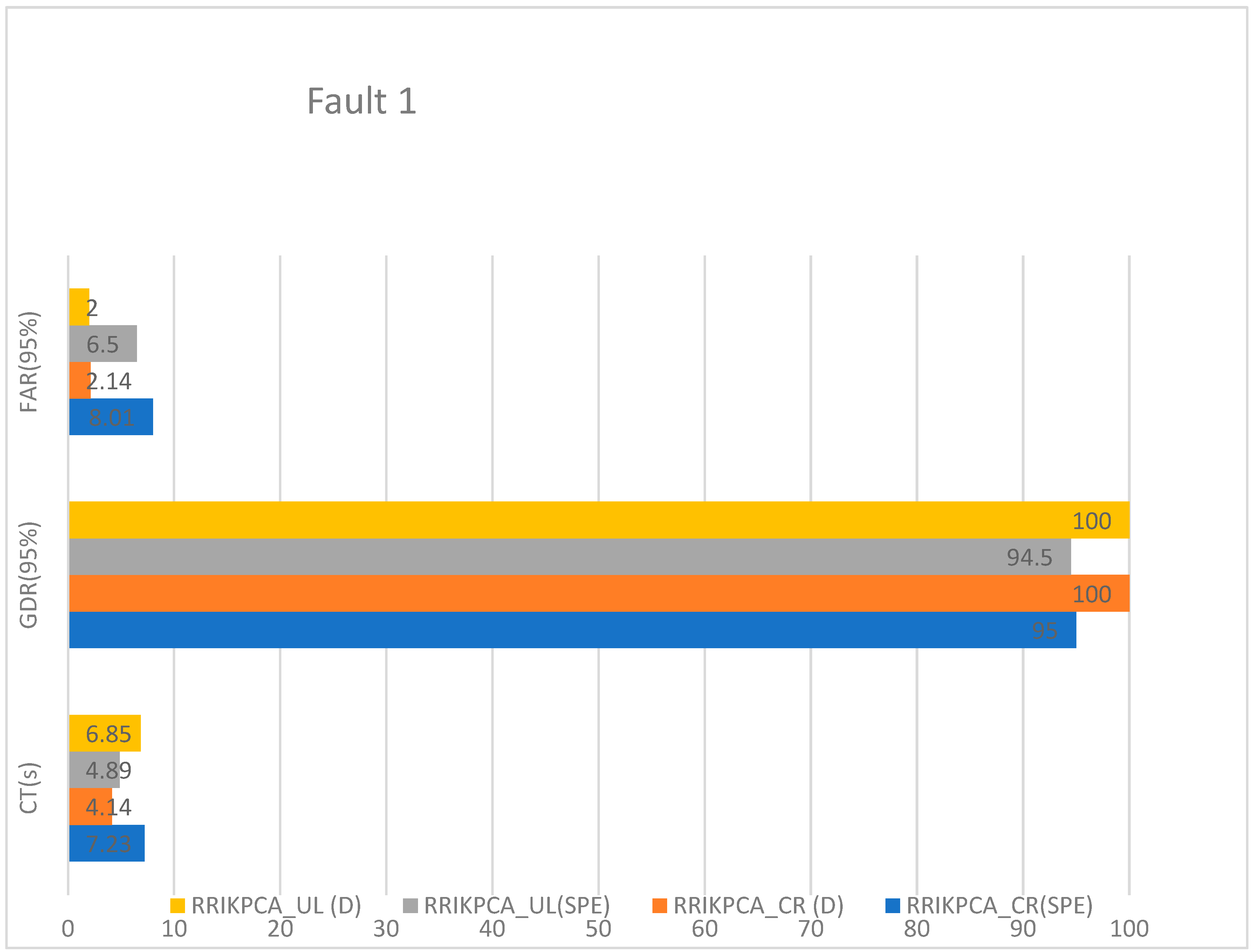
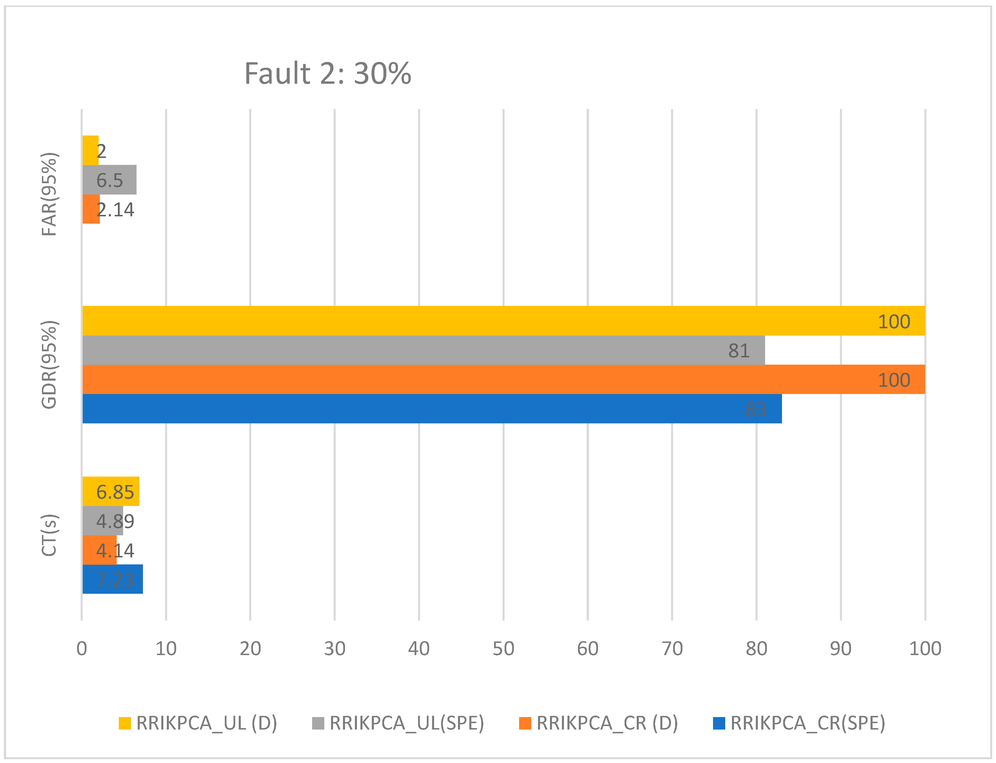
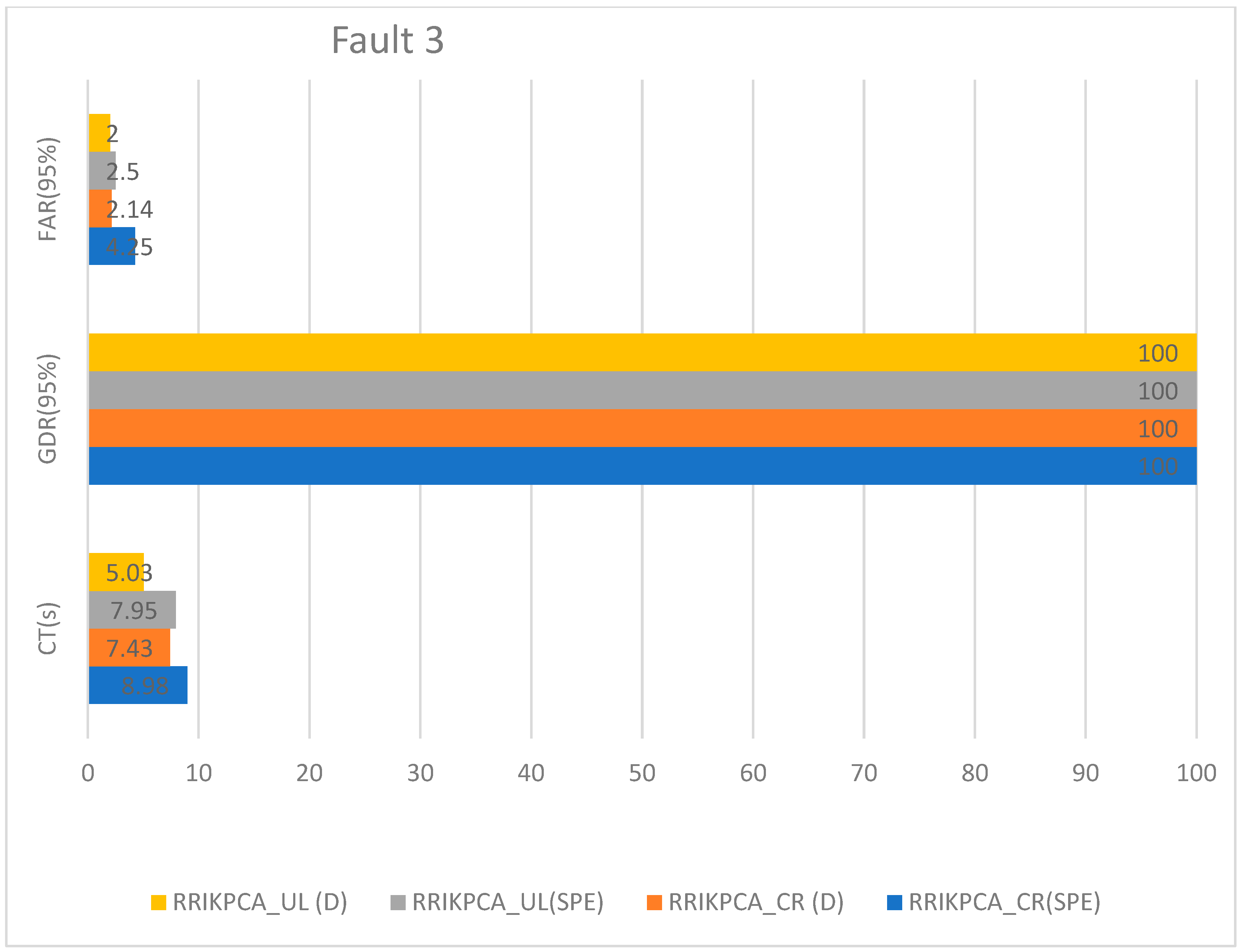
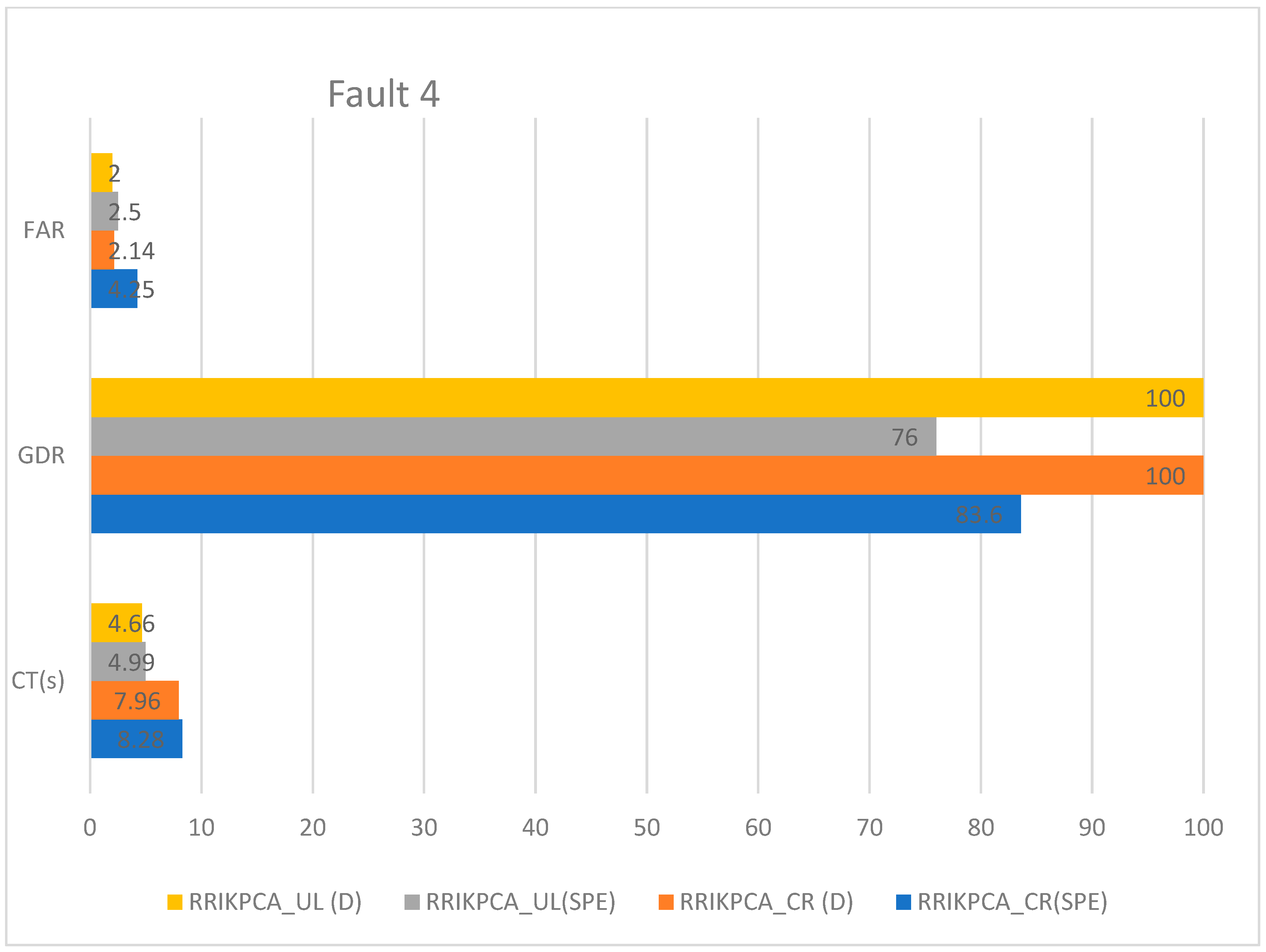
The first part of the analysis focuses on the fault detection capability of the different indices. As shown in Figure 3, Figure 4, Figure 5 and Figure 6, methods based on the proposed index consistently outperform those relying on the classical SPE statistic. This behavior can be explained by the fact that SPE is computed in the residual subspace and may dilute fault information when uncertainty and nonlinear effects are present, especially under interval modeling. In contrast, the proposed index exploits the most sensitive residual components, making it more responsive to fault-induced variations.

Among all tested approaches, the RRIKPCA_CR method based on $D_{4CR}$ achieves the best overall performance. It maintains a 100% GDR for all fault scenarios, while simultaneously achieving the lowest FAR. In addition, its computation time remains low. This improved efficiency is attributed to the center–range (CR) interval representation, which preserves essential uncertainty information while reducing redundant computations compared to the upper–lower (UL) formulation.

Although the RRIKPCA_UL approach based on [D₄] also attains a perfect GDR, its computation time is slightly higher in several scenarios, indicating that the CR formulation offers a better compromise between detection accuracy and computational efficiency. In contrast, SPE-based methods exhibit higher FAR values and reduced detection reliability in certain fault conditions, highlighting their limited sensitivity in uncertain and nonlinear environments.

This difference is particularly evident in the case of fault 4 (Figure 6). Despite the introduction of a severe fault corresponding to a 40% increase in the standard deviation of the O₃ signal, the SPE-based methods fail to provide satisfactory detection, as reflected by reduced GDR values in both UL and CR configurations. Such detection uncertainty is unacceptable in air quality monitoring applications, where delayed or missed detection may have direct health implications. Conversely, the proposed $D_{4CR}$ index achieves a perfect GDR of 100%, confirming its superior fault sensitivity and robustness.

Table 3. Fault detection performances of RR-IKPCA based on [SPE] and [D₄].

Methods	Fault 1			Fault 2			Fault 3			Fault 4
	FAR 95%	GDR 95%	CT(s)	FAR 95%	GDR 95%	CT(s)	FAR 95%	GDR 95%	CT(s)	FAR 95%	GDR 95%	CT(s)
RRKPCA based on SPE	5	74	4.5	3.8	88	9	4.18	90	5.23	4	74	4.89
RRKPCA based on D4	3.8	90	4.14	2.29	91	2	2.5	96	5	2.5	80	4.66
RRIKPCA_UL based on [SPE]	6.8	94.5	4.89	6.5	81	4.89	2.5	100	7.95	2.5	76	4.99
RRIKPCA_UL based on [D4]	2	100	6.85	2	100	6.85	4.25	100	5.03	2	100	4.66
RRIKPCA_CR based on [SPE]	8.01	95	4.14	5	83	7.23	8.98	100	8.98	4.25	83.6	4.99
RRIKPCA_CR based on [D4]	2.4	100	7.23	2.4	100	4.14	7.89	100	7.43	2.14	100	7.96

presents a comparative study between the [SPE] and [D] indices in order to determine the most appropriate choice for fault detection, which consequently leads to better fault isolation. It is clear that the proposed index outperforms the others due to the superior results obtained.

Furthermore, this table presents a comparative analysis of different fault detection and localization methods under two operating conditions: ideal measurements without uncertainty (0%) and noisy measurements with 2% uncertainty. The comparison was conducted to evaluate the sensitivity and robustness of each method when measurement uncertainty is introduced. As shown in the table, the addition of uncertainty generally affects the fault attribution and detection performance of the conventional approaches, leading to higher false alarm rates and reduced localization reliability. In contrast, the proposed RR-IKPCA-based framework maintains more stable performance with comparatively lower FAR values and clearer fault isolation capability under uncertain conditions. These results demonstrate that the proposed method is less sensitive to measurement variations and remains effective in realistic air quality monitoring environments where sensor noise and uncertainty are unavoidable.

All experiments were conducted on a MSI GF63 Thin 10SC laptop equipped with an Intel^® Core™ i7-10750H processor operating at 2.60 GHz, 16 GB RAM, and Intel^® UHD Graphics with 8 GB shared memory. The implementation and simulations were performed in a Windows 10 Professional 64-bit environment with DirectX 12 support. The reported computation time (CT) values were obtained under this hardware and software configuration to ensure reproducibility and provide a representative evaluation of the computational performance of the proposed method.

To summarize, the simulation results clearly demonstrate that combining the elimination-based localization principle with the proposed sensitive detection index significantly enhances fault detection and localization performance. Compared with the classical SPE-based approach, the proposed method provides clearer fault attribution, lower false alarm rates, and higher detection reliability under interval uncertainty and nonlinear system behavior. The reduction in diagnostic ambiguity is particularly evident when the faulty variable is eliminated, which leads to a pronounced decrease in the detection index and enables unambiguous localization. These results confirm that the proposed index is better suited than SPE for elimination-based localization and highlight the effectiveness of the RR-IKPCA_CR framework in uncertain air quality monitoring applications.

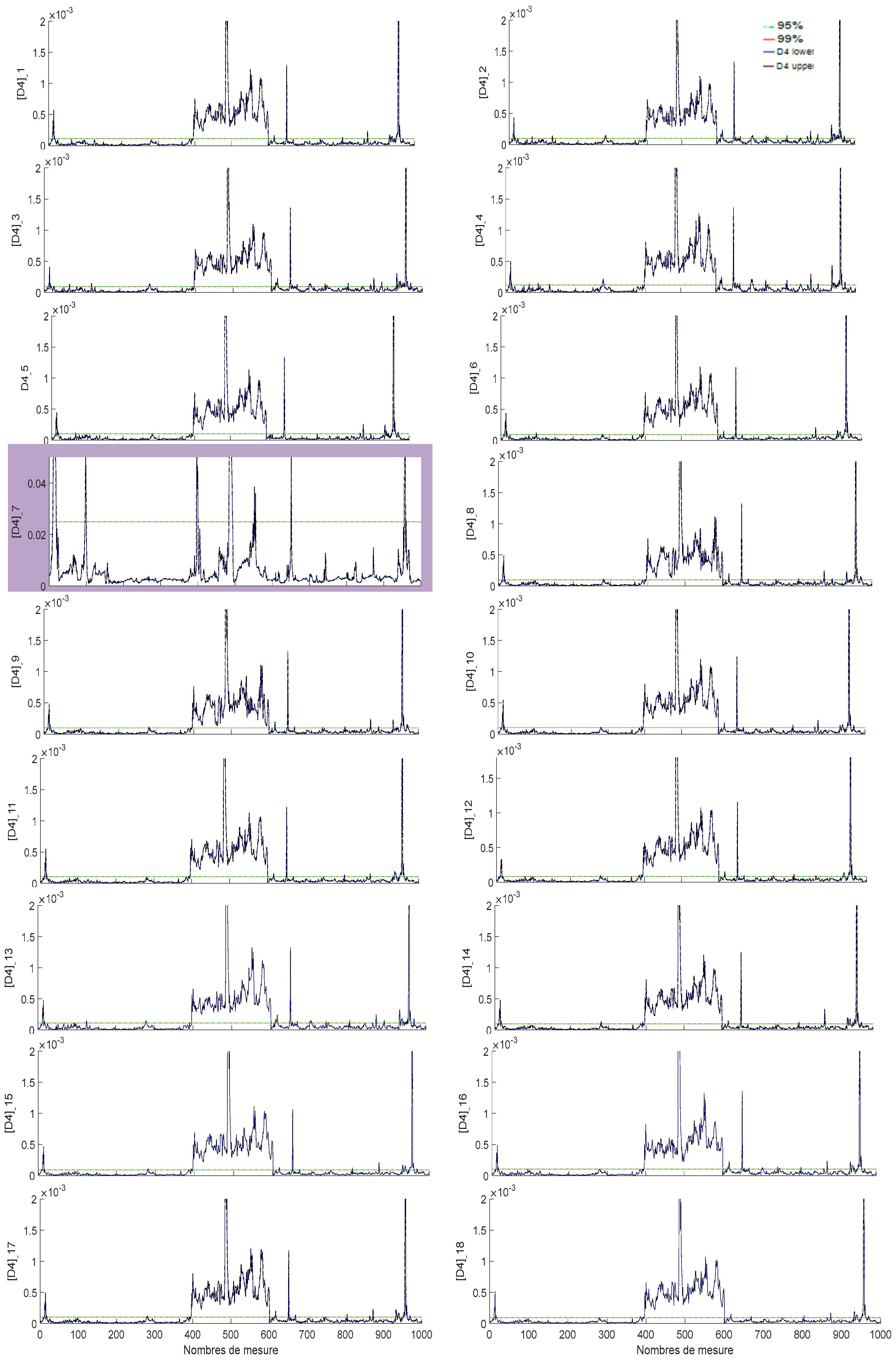
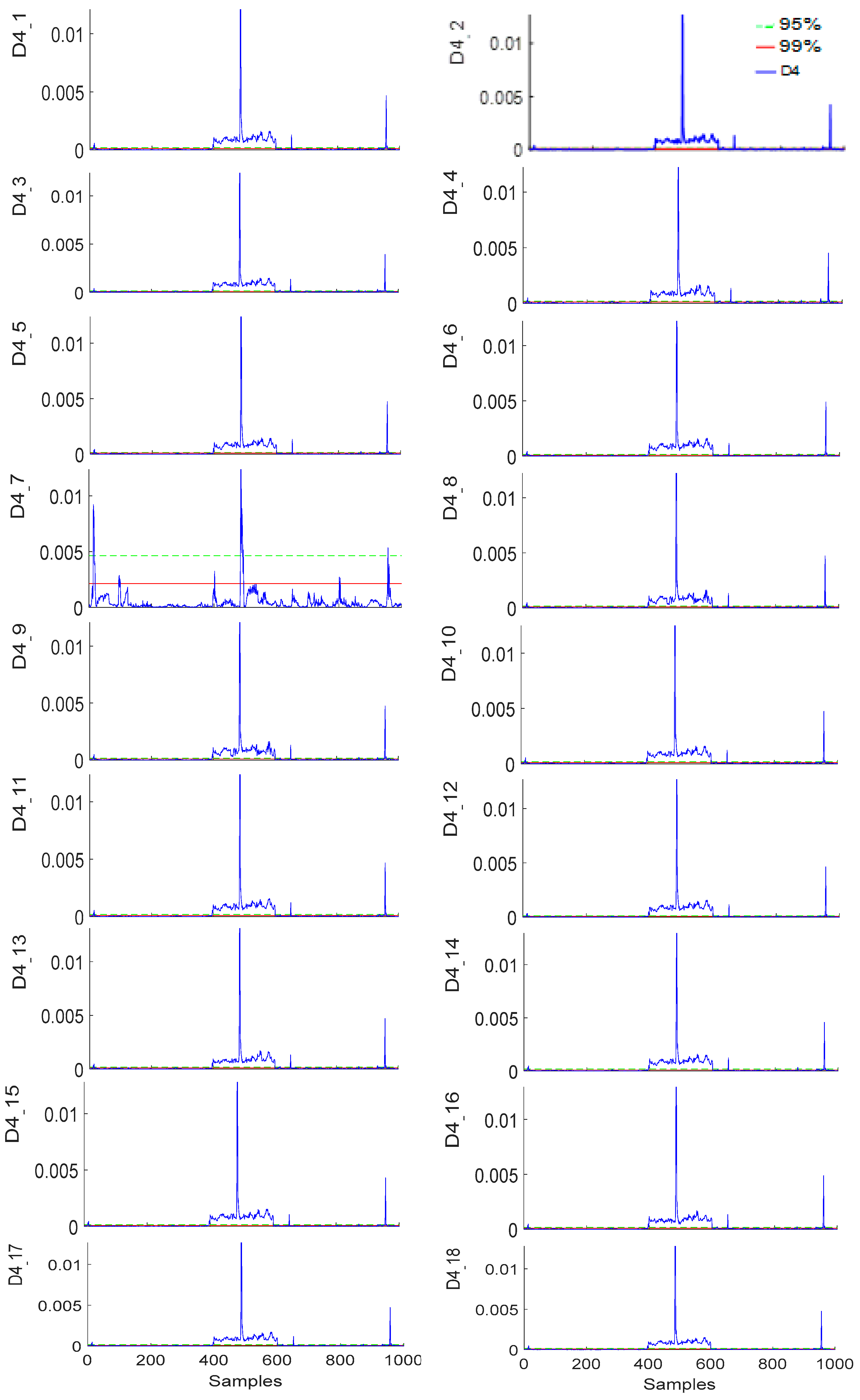
Figure 7 and Figure 8 show the fault localization results by elimination for fault (d7), using the two models: RR-IKPCA-UL with the index [D4] and RR-IKPCA- CR with the index D_4CR, respectively. The evolution of different ${\left[D_4\right]}_{-j}$ and $D_{{4CR}_{-j}}$ values in the case of fault (d7) shows that eliminating variable v7 leads to the indices ${\left[D_4\right]}_{-7}$ and $D_{4_{-7}}$, which no longer indicate the presence of the fault. Figure 9 and Figure 10 present the Qr ratio for each of the 18 models. These figures show that the smallest ratio corresponds to variable v7, indicating that this variable is the source of the fault.

To summarize, this approach aims to locate the faulty variable by analyzing how the detection index behaves when each variable is individually removed. The use of RR-IKPCA and interval analysis makes the fault diagnosis more robust and reliable, especially under uncertainty.

5.2. Comparative Analysis

To position the proposed method with respect to existing approaches,

Table 4. Comparative analysis.

Method	Model Type	Localization Principle	Uncertainty Handling	Strengths	Main Limitations	Detection Rate	References
Partial contribution	Linear PCA	Contribution of each variable to (T2) or SPE	No	Simple to implement; intuitive interpretation	Smearing effect; poor localization for correlated variables	84.5	[44]
Reconstruction-based contribution (RBC)	Linear PCA + Nonlinear (KPCA)	Variable-wise reconstruction error	No	Improved localization compared with contribution plots	Sensitive to noise; linear assumption; no uncertainty modeling	89.7	[35,39,45,46]
Partial reconstruction (PR)	Linear PCA	Reconstruction of selected variables	No	Better discrimination than classical RBC	Increased computational burden; linear assumption	91.2	[32]
Proposed RRIKPCA + elimination	Nonlinear (IKPCA)	Elimination-based diagnostic ratio using sensitive residual index	Yes (interval-based)	High fault sensitivity; robust to uncertainty; clear localization	Assumes single dominant fault; higher complexity for large-scale systems	97.8	This work

shows a comparison between commonly used fault localization techniques in terms of model type, localization principle, uncertainty handling, and limitations.

In practical industrial systems, the assumption of a single-fault occurrence may not always hold, as multiple faults can arise simultaneously under complex operating conditions. In such scenarios, the separation and identification of individual fault signatures become more challenging, potentially affecting the localization accuracy of the proposed RR-IKPCA framework. Although the current study focuses on single-fault scenarios to establish the effectiveness of the method, we acknowledge that multi-fault conditions represent a more realistic and demanding case. The behavior of the proposed approach under simultaneous faults is therefore an important consideration, and its detailed investigation, including performance evaluation and possible methodological extensions to handle fault overlap, is identified as a relevant direction for future research.

6. Conclusions

This paper proposes a fault detection and localization method for diagnosing sensor failures in an air monitoring network by combining interval-based fault detection techniques with the localization-by-elimination principle. The effectiveness of the proposed approach is demonstrated through its application to fault diagnosis in an air quality monitoring network. Quantitative results obtained from the AIRLOR air quality monitoring network demonstrate the effectiveness of the proposed method. The RRIKPCA_CR-based localization scheme achieved a good detection rate (GDR) across all tested fault scenarios, while maintaining a low false alarm rate (FAR).

Despite the promising results, the proposed framework has several limitations. It assumes that faults occur independently and relies on the availability of sufficient historical data for effective model training. Furthermore, the current implementation has not yet been validated under simultaneous multiple-fault conditions or highly dynamic operating environments. Future work will therefore focus on extending the framework to handle multiple concurrent faults, time-varying process dynamics, and adaptive or online learning schemes. In addition, applying the proposed approach to other domains such as water quality monitoring and industrial process control will further evaluate its generality and scalability.

References

1. Isermann, R. Fault-Diagnosis Systems: An Introduction from Fault Detection to Fault Tolerance; Springer Science & Business Media: London, UK, 2005. [Google Scholar]
2. Chiang, L.H.; Russell, E.L.; Braatz, R.D. Fault Detection and Diagnosis in Industrial Systems; Springer Science and Business Media LLC: London, UK, 2001. [Google Scholar]
3. Blanke, M.; Kinnaert, M.; Lunze, J.; Staroswiec, M. Diagnosis et Fault-Tolerant Control; Springer: Berlin/Heidelberg, Germany, 2003. [Google Scholar]
4. Zhu, Y.; Zhao, S.; Zhang, Y.; Zhang, C.; Wu, J. A Review of Statistical-Based Fault Detection and Diagnosis with Probabilistic Models. Symmetry 2024, 16, 455. [Google Scholar] [CrossRef] [Scilit]
5. Jolliffe, I.T. Principal Component Analysis; Springer: Berlin/Heidelberg, Germany, 2002. [Google Scholar]
6. Wang, J.; Zhou, Z.; Li, Z.; Du, S. A novel fault detection scheme based on mutual k-nearest neighbor method: Application on the industrial processes with outliers. Processes 2022, 10, 497. [Google Scholar] [CrossRef] [Scilit]
7. Janssen, S.; Dumont, G.; Fierens, F.; Deutsch, F.; Maiheu, B.; Celis, D.; Trimpeneers, E.; Mensink, C. Land use to characterize spatial representativeness of air quality monitoring stations and its relevance for model validation. Atmos. Environ. 2012, 59, 492–500. [Google Scholar] [CrossRef] [Scilit]
8. Harkat, M.-F.; Mansouri, M.; Nounou, M.; Nounou, H. Enhanced data validation strategy of air quality monitoring network. Environ. Res. 2018, 160, 183–194. [Google Scholar] [CrossRef] [Scilit] [PubMed]
9. Fazai, R.; Abdellafou, K.B.; Said, M. Online fault detection and isolation of an AIR quality monitoring network based on machine learning and metaheuristic methods. Int. J. Adv. Manuf. Technol. 2018, 99, 2789–2802. [Google Scholar] [CrossRef] [Scilit]
10. Harkat, M.-F.; Mourot, G.; Ragot, J. An improved PCA scheme for sensor FDI: Application to an air quality monitoring network. J. Process Control 2006, 16, 625–634. [Google Scholar] [CrossRef] [Scilit]
11. Ge, Z.; Song, Z.; Gao, F. Review of recent research on data-based process monitoring. Ind. Eng. Chem. Res. 2013, 52, 3543–3562. [Google Scholar] [CrossRef] [Scilit]
12. Xie, Z. Identification of sensor fault characteristics based on adaptive kernel principal component analysis. Eur. J. Eng. Technol. 2025, 1, 7–15. [Google Scholar]
13. Hamrouni, I.; Lahdhiri, H.; Ben Abdellafou, K.; Aljuhani, A.; Taouali, O.; Bouzrara, K. Anomaly Detection and Localization for Process Security Based on the Multivariate Statistical Method. Math. Probl. Eng. 2022, 2022, 5580774. [Google Scholar] [CrossRef] [Scilit]
14. Samuel, R.T.; Cao, Y. Nonlinear process fault detection and identification using kernel PCA and kernel density estimation. Syst. Sci. Control Eng. 2016, 4, 165–174. [Google Scholar] [CrossRef] [Scilit]
15. Gharahbagheri, H.; Imtiaz, S.A.; Khan, F. Root cause diagnosis of process fault using KPCA and Bayesian network. Ind. Eng. Chem. Res. 2017, 56, 2054–2070. [Google Scholar] [CrossRef] [Scilit]
16. Wang, Q.; Liu, Y.B.; He, X.; Liu, S.Y.; Liu, J.H. Fault diagnosis of bearing based on KPCA and KNN method. Adv. Mater. Res. 2014, 986–987, 1491–1496. [Google Scholar] [CrossRef] [Scilit]
17. Zheng, D.; Zhou, L.; Song, Z. Kernel generalization of multi-rate probabilistic principal component analysis for fault detection in nonlinear process. IEEE/CAA J. Autom. Sin. 2021, 8, 1465–1476. [Google Scholar] [CrossRef] [Scilit]
18. Zhang, Q.; Li, P.; Lang, X.; Miao, A. Improved dynamic kernel principal component analysis for fault detection. Measurement 2020, 158, 107738. [Google Scholar] [CrossRef] [Scilit]
19. Benkouider, M.S.B. Sensor fault detection using a new online reduced rank kernel PCA for monitoring an air quality monitoring network. Control Eng. Pract. 2020, 103, 104543. [Google Scholar]
20. Box, G.E.P. Some theorems on quadratic forms applied in the study of analysis of variance problems, I. effect of inequality of variance in the one-way classification. Ann. Math. Stat. 1954, 25, 290–302. [Google Scholar] [CrossRef] [Scilit]
21. Ait-Izem, T.; Harkat, M.-F.; Djeghaba, M.; Kratz, F. On the application of interval PCA to process monitoring: A robust strategy for sensor FDI with new efficient control statistics. J. Process Control 2018, 63, 29–46. [Google Scholar] [CrossRef] [Scilit]
22. Cazes, P.; Chouakria, A.; Diday, E.; Schektman, Y. Extension de l’Analyse en Composantes principales à des données de Type Intervalle. Rev. Stat. Appliquée 1997, 45, 5–24. [Google Scholar]
23. Chouakria, A. Extension des Méthodes d’analyse Factorielle à des Données de Type Intervalle. Ph.D. Thesis, Université des Sciences et Technologies de Lille, Lille, France, 1998. [Google Scholar]
24. Mansouri, M.; Harkat, M.-F.; Nounou, M.; Nounou, H. Midpoint-radii principal component analysis-based EWMA and application to air quality monitoring network. Chemom. Intell. Lab. Syst. 2018, 175, 55–64. [Google Scholar] [CrossRef] [Scilit]
25. Le-Rademacher, J.; Billard, L. Symbolic Covariance Principal Component Analysis and Visualization for Interval Valued Data. J. Comput. Graph. Stat. 2012, 21, 413–432. [Google Scholar] [CrossRef] [Scilit]
26. Chakour, C.; Benyounes, A.; Boudiaf, M. Diagnosis of uncertain nonlinear systems using interval kernel principal components analysis: Application to a weather station. ISA Trans. 2018, 83, 126–141. [Google Scholar] [CrossRef] [Scilit]
27. Hamrouni, I.; Lahdhiri, H.; Abdellafou, K.; Taouali, O. Fault detection of uncertain nonlinear process using Reduced Interval Kernel Principal Component Analysis (RIKPCA). Int. J. Adv. Manuf. Technol. 2020, 106, 4567–4576. [Google Scholar] [CrossRef] [Scilit]
28. Hamrouni, I.; Abdellafou, K.B.; Aborokbah, M.; Taouali, O. Dynamic sensor fault detection approach using data-driven techniques. Neural Comput. Appl. 2024, 36, 14291–14307. [Google Scholar] [CrossRef] [Scilit]
29. Lahdhiri, H.; Taouali, O. Interval valued data driven approach for sensor fault detection of nonlinear uncertain process. Measurement 2021, 171, 108776. [Google Scholar] [CrossRef] [Scilit]
30. Harkat, M.; Mansouri, M.; Nounou, M.; Nounou, H. Fault detection of uncertain chemical processes using interval partial least squares-based generalized likelihood ratio test. Inf. Sci. 2019, 490, 265–284. [Google Scholar] [CrossRef] [Scilit]
31. Alcala, C.F. Fault Diagnosis with Reconstruction Based Contributions for Statistical Process Monitoring. Ph.D. Thesis, University of Southern California (USC), Los Angeles, CA, USA, 2011. [Google Scholar]
32. Harakat, M.F. Détection et Localisation de Défauts par Analyse en Composantes Principales. Ph.D. Thesis, National Polytechnic Institute of Lorraine, Nancy, France, 2003. [Google Scholar]
33. Brunet, J.; Labarrère, M.; Jaume, D.; Rault, A.; Vergé, M. Détection et Diagnostic de Pannes: Approche par Modélisation; Hermès: Paris, France, 1990. [Google Scholar]
34. Jafari, N.; Lopes, A.M. Fault Detection and Identification with Kernel Principal Component Analysis and Long Short-Term Memory Artificial Neural Network Combined Method. Axioms 2023, 12, 583. [Google Scholar] [CrossRef] [Scilit]
35. Alcala, C.F.; Qin, S.J. Reconstruction-based contribution for process monitoring with kernel principal component analysis. Ind. Eng. Chem. Res. 2010, 49, 7849–7857. [Google Scholar] [CrossRef] [Scilit]
36. Shahzad, F.; Huang, Z.; Memon, W.H. Process Monitoring Using Kernel PCA and Kernel Density Estimation-Based SSGLR Method for Nonlinear Fault Detection. Appl. Sci. 2022, 12, 2981. [Google Scholar] [CrossRef] [Scilit]
37. Wang, H.; Peng, M.-J.; Yu, Y.; Saeed, H.; Hao, C.-M.; Liu, Y.-K. Fault identification and diagnosis based on KPCA and similarity clustering for nuclear power plants. Ann. Nucl. Energy 2021, 150, 107786. [Google Scholar] [CrossRef] [Scilit]
38. Fezai, R.; Mansouri, M.; Trabelsi, M.; Hajji, M.; Nounou, H.; Nounou, M. Online reduced kernel GLRT technique for improved fault detection in photovoltaic systems. Energy 2019, 179, 1133–1154. [Google Scholar] [CrossRef] [Scilit]
39. Lahdhiri, H.; Aljuhani, A.; Ben Abdellafou, K.; Taouali, O. An Improved Fault Diagnosis Strategy for Process Monitoring Using Reconstruction Based Contributions. IEEE Access 2021, 9, 79520–79533. [Google Scholar] [CrossRef] [Scilit]
40. Zeng, L.; Long, W.; Li, Y. A Novel Method for Gas Turbine Condition Monitoring Based on KPCA and Analysis of Statistics T2 and SPE. Processes 2019, 7, 124. [Google Scholar] [CrossRef] [Scilit]
41. Mansouri, M.; Nounou, M.; Nounou, H.; Karim, N. Kernel PCA-based GLRT for nonlinear fault detection of chemical processes. J. Loss Prev. Process Ind. 2016, 40, 334–347. [Google Scholar] [CrossRef] [Scilit]
42. Stork, C.L.; Veltkamp, D.J.; Kowalski, B.R. Identification of multiple sensor disturbances during process monitoring. Anal. Chem. 1997, 69, 5031–5036. [Google Scholar] [CrossRef] [Scilit]
43. Dunia, R.; Qin, S.J.; Edgar, T.F.; McAvoy, T.J. Identification of faulty sensors using principal component analysis. AIChE J. 1996, 42, 2797–2812. [Google Scholar] [CrossRef] [Scilit]
44. Wang, Z.; Cheng, J.; Liu, W.; Zou, X.; Tao, F. A fault localization approach based on multi-system PCA and dynamic SDG: Application in train lifting equipment. Robot. Comput.-Integr. Manuf. 2024, 2024, 102694. [Google Scholar] [CrossRef] [Scilit]
45. Zhou, W.; Yang, W.; Wang, Y.; Zhang, H. Generalized reconstruction-based contribution for multiple faults diagnosis with bayesian decision. In Proceedings of the 2018 IEEE 7th Data Driven Control and Learning Systems Conference (DDCLS), Enshi, China, 25–27 May 2018; pp. 813–818. [Google Scholar]
46. Ziane, A.; Mekhilef, S.; Dabou, R.; Sahouane, N.; Necaibia, A.; Rouabhia, A.; Khelifi, S.; Lachter, S.; Mostefaoui, M.; Larbi, A.A.; et al. Online fault detection in grid-connected PV system using nonlinear multivariate statistical analysis. Electr. Eng. 2026, 108, 107. [Google Scholar] [CrossRef] [Scilit]
Figure 1. RR-IKPCA based on interval midpoint–radii.
Applsci 16 05674 g001
Figure 2. RR-IKPCA upper–lower bound.
Applsci 16 05674 g002
Figure 3. Fault detection performance for RR-IKPCA based on [SPE] and [D]; fault 1.
Applsci 16 05674 g003
Figure 4. Fault detection performance for RR-IKPCA based on [SPE] and [D]; fault 2.
Applsci 16 05674 g004
Figure 5. Fault detection performance for RR-IKPCA based on [SPE] and [D]; fault 3.
Applsci 16 05674 g005
Figure 6. Fault detection performance for RR-IKPCA based on [SPE] and [D4]; fault 4.
Applsci 16 05674 g006
Figure 7. Time evolution of D 4 obtained using the elimination method based on RR−IKPCA−UL model with fault 4.
Applsci 16 05674 g007
Figure 8. Time evolution of D 4 C R obtained using the elimination method based on RR-IKPCA-CR model with fault 4.
Applsci 16 05674 g008
Figure 9. Fault location using report Q r using the elimination method based on RR-IKPCA-UL model.
Applsci 16 05674 g009
Figure 10. Fault location using interval report Q r using the elimination method based on RR-IKPCA-UL model.
Applsci 16 05674 g010