System-Level Modeling of Parabolic Solar Dish–Stirling Units with Explicit Loss Partitioning Under Variable Charge Control

Abstract

Parabolic solar dish–Stirling (PSDS) technologies are among the most efficient solar-to-electric conversion options, but their system-level modeling remains challenging because optical losses, receiver heat losses, package leakage, and Stirling engine non-idealities are strongly coupled under variable operating conditions. This study develops a modular, energy-consistent system-level framework that couples dish receiver optics and thermal behavior, hot-end package losses, and a non-ideal Stirling engine under variable charge (Qu-mode) control. The key novelty is a receiver engine heat-matching formulation in which receiver temperature, useful heat, working gas charge/mean pressure, and engine output emerge from a closed energy balance rather than from prescribed hot-side temperature, fixed heat input, or prescribed mean pressure. The framework was benchmarked in stages against the Mendoza receiver formulation, GPU-3/LeRC Stirling engine data, and EuroDish dispatch-level measurements. At the integrated EuroDish level, it reproduced heat input, cooler rejection, and net electrical output with mean absolute percentage errors of 2.90%, 4.07%, and 4.28%, respectively, while preserving explicit traceability of optical, receiver, package, engine, generator, and parasitic losses. A receiver formulation comparison showed that the final receiver treatment reduced the cooler rejection MAPE from 8.11% to 4.07% relative to the Mendoza-type receiver swap baseline. A limited-input transferability study for representative pressure-controlled dish–Stirling platforms retained peak power and efficiency within a ±10% envelope for the quantitatively assessed cases. Parametric studies further showed a broad engine speed optimum, a heat exchanger sizing trade-off governed by conductance and pumping/friction losses, stronger sensitivity to ambient temperature than wind over the tested EuroDish range, and cooling boundary effects that redirect fixed thermal input from electricity to rejected heat. The resulting framework provides a compact predictive basis for loss diagnosis, design studies, and control-oriented evaluation of PSDS units.

1. Introduction

The abundance of solar thermal power makes it an attractive renewable energy source for generating both thermal and electrical energy in power plants of all sizes. By integrating solar thermal energy with a solar parabolic dish and a Stirling engine, one can convert thermal energy into electric energy. Likewise, solar energy can be effectively transformed into multiple outputs, including heat, electricity, and energy vectors [1,2,3]. In terms of efficiency, parabolic solar dish–Stirling (PSDS) technologies are considered the most efficient solar-to-electric conversion options [4], exhibiting nearly 30% higher power density compared to other Concentrated Solar Power (CSP) technologies. They also feature hybrid operation, modularity, flexibility, capability to reach high temperature ranges, and a long lifespan [4,5,6]. Another notable benefit of PSDS is that it provides electricity directly, bypassing the need for a turbine. This combination of properties has made them the most suitable contenders for generating electricity that is both economically viable and environmentally friendly. Indeed, their adoption has led to a reduction in capital costs and, consequently, in the Levelized Cost of Energy (LCOE) [2,6].

Thermal energy storage (TES) is also becoming increasingly relevant for dish–Stirling and hybrid solar–thermal systems because it can buffer the mismatch between solar availability, power demand, and secondary thermal loads. Recent reviews highlight the rapid development of phase change materials (PCMs), nano-enhanced PCMs, encapsulated PCMs, and hybrid PCM/nanomaterial systems for solar–thermal storage, waste heat recovery, and improved charging/discharging behavior [7,8]. These materials can increase effective thermal conductivity, improve heat transfer rates, enhance thermal reliability over repeated cycles, and support more compact latent heat storage architectures. At the broader solar–thermal level, polygeneration systems can combine power, desalination, and cooling [1], while dish–Stirling-specific hybrid studies have used Stirling-rejected heat or exhaust heat for desalination, additional electricity, cooling production and storage-assisted operation [3,9]. This context motivates the need for a loss-resolved receiver engine model that can quantify not only net electricity but also cooler rejection and other recoverable heat streams.

Given the complexity of these sustainable co-generation systems, predictive system-level models are a critical element in system analysis and design. They are required for steps such as (i) diagnosing dominant loss channels and operational constraints, (ii) ensuring design optimization (receiver/aperture sizing, insulation, heat exchanger sizing), and (iii) establishing the control strategies (mean pressure/working gas mass regulation, speed control) suitable for variable irradiance and ambient conditions [10,11,12,13]. Yet all types of available models [14,15] are either too detailed and platform-specific for repeated design studies, too simplified to provide trustworthy loss partitioning under changing DNI, wind, and ambient temperature, or too aggregated to enforce a closed receiver–engine heat match under a realistic operating point control strategy.

In the case of high-fidelity, system-specific models, while they can resolve receiver radiative exchange (often via radiosity/view factors) and employ detailed engine representations, enabling deep energy balance insight for a given platform (e.g., EuroDish/SOLO-161 class studies) [10], they are typically computationally heavy and closely tied to a particular geometry and calibration dataset [16]. As for design-oriented receiver frameworks, their ability to provide closed-form or semi-empirical relations for receiver temperature and losses makes them well suited for early stage sizing and sensitivity studies. But they typically require simplified engine representations and do not provide full thermodynamic coupling [17,18]. They further necessitate maintaining a closed receiver engine energy balance in order to separate environment-driven receiver behavior (wind/ambient effects) from engine operating point changes managed by active control. Dedicated Stirling engine models, which range from classical adiabatic analyses to more advanced computational formulations [19,20], including non-ideal adiabatic models with explicit loss accounting (e.g., Araoz et al. [21]), are typically utilized with fixed solar receiver boundary conditions rather than dynamically varying solar inputs. Reduced-order control and grid-oriented models, which prioritize computational speed and capture average behavior for receiver temperature and mean pressure control, excel at grid integration and stability analysis (e.g., [11,12,13,22]) but generally sacrifice receiver geometry fidelity and detailed thermodynamic loss partitioning. Validated steady or quasi-steady complete-system models [2,23,24,25] are useful for planning, optimization, and comparative performance evaluation, but they generally rely on more aggregated component descriptions and do not explicitly resolve receiver/package/engine loss propagation under a control-consistent heat match solution. While hybrid and extended system-level configurations broaden the scope further to multi-source or multi-output architectures [3,26], they likewise do not remove the practical need for a modular, energy-consistent, EuroDish-class PSDS framework with explicit receiver/package/engine coupling and validated dispatch-level loss partitioning.

Another option is experimental performance analyses, such as the EuroDish study by Reinalter et al. [5], which provide an essential benchmark by reporting a system energy balance derived from measurements combined with modeled/estimated sub-terms (e.g., package heat ingress and parasitics). Although extremely valuable for validation, given that some balance entries are not uniquely measured, these datasets do not by themselves provide a complete predictive model for extrapolation across operating regimes.

As summarized in

Table 1. Summary of representative published studies and remaining modeling gaps relevant to the present PSDS framework.

Study Class	Representative Studies	Main Capability	Remaining Gap Relative to the Present Objectives
EuroDish measurements and system-specific studies	Reinalter et al. [5]; Nepveu et al. [10]; detailed EuroDish/SOLO-161 studies [16]	Provide benchmark data, measured/estimated loss taxonomy, and detailed platform-specific insight	Closely tied to a specific system and calibration dataset; limited direct use as a compact reusable design/control model
Design-oriented receiver and opto-geometric models	Mendoza et al. [17]; receiver/sizing studies [18]	Describe dish optics, receiver sizing, cavity losses, and receiver thermal behavior	Usually use simplified engine coupling and do not resolve non-ideal Stirling operation under receiver engine heat matching
Standalone Stirling engine models	Urieli–Berchowitz [19]; Dyson [20]; Araoz et al. [21]	Provide adiabatic/non-ideal Stirling thermodynamics, cycle losses, and engine-side performance prediction	Often require prescribed hot-side boundary conditions rather than a receiver-coupled heat input and operating point solution
Reduced-order and control-oriented PSDS models	Control/grid-oriented models [11,12,13,22]	Capture fast system response, receiver temperature behavior, mean pressure control, or grid/control behavior	Generally reduce receiver geometry and detailed loss channel resolution
Complete-system performance and optimization models	System-level and optimization studies [2,23,24,25]	Support planning, optimization, and comparative performance evaluation	Often use aggregated component descriptions and limited receiver/package/engine loss propagation
Hybrid, polygeneration, and TES-related solar–thermal studies	Solar polygeneration [1]; dish/Stirling hybrid systems [3,9]; TES/PCM reviews [7,8]	Extend solar–thermal systems toward desalination, cooling, additional power recovery, rejected heat utilization, and storage	Require a reliable loss-resolved receiver engine core to quantify electricity, cooler rejection, and recoverable heat streams consistently

, the remaining gap is not the absence of receiver models, Stirling engine models, or system-level PSDS studies individually. Rather, the gap is the lack of a compact framework that simultaneously couples a EuroDish-class dish/receiver/package front-end to a non-ideal Stirling engine model, enforces receiver engine heat matching under variable charge operation, and preserves explicit loss channel propagation from optical capture to net electrical output and cooler rejection. This gap is important for design studies, control-oriented simulations, and hybrid/TES evaluations, where both electrical output and rejected/recoverable heat streams must be quantified consistently.

To address this gap, this work develops a modular, computationally efficient, energy-consistent Non-ideal Mean-Pressure-Regulated Parabolic Dish–Stirling (NIMP-PSDS) framework. The framework builds on and adapts the Mendoza et al. dish/receiver formulation as the solar front-end basis [17], incorporates the Reinalter/Nepveu EuroDish/ SOLO-161 reference geometry and loss taxonomy [5,10], and uses the Urieli–Berchowitz/Araoz et al. adiabatic and non-ideal Stirling engine formulations as the engine thermodynamic core [19,21]. In the present implementation, these elements are extended through EuroDish-specific receiver anchoring, a view-factor-weighted aperture emission treatment, an explicit receiver-to-package loss channel, variable charge operating point iteration, and engine-side loss/conductance updates. The resulting coupled framework represents mean pressure regulation in a manner consistent with variable-pressure control strategies reported for kinematic Stirling engines [4,10,27]. It therefore provides end-to-end energy flow closure from DNI to net electrical output, while retaining intermediate heat flow and loss terms such as receiver losses, package leakage, engine heat input, cooler rejection, generator conversion, and parasitic consumption.

Accordingly, the objective of this study is to develop, validate, and demonstrate a compact NIMP-PSDS framework for loss-resolved analysis of EuroDish-class and related pressure-controlled parabolic dish–Stirling systems under variable charge operation. The novelty is threefold: (i) a receiver/package/non-ideal Stirling coupling strategy that links the dish/receiver front-end to the engine hot-side boundary; (ii) explicit loss traceability across optical, receiver, package, engine, generator, parasitic, and cooler rejection channels; and (iii) a Qu-mode receiver engine heat-matching solution that determines the coupled system operating point from receiver/package heat availability and Stirling engine thermal demand rather than from prescribed hot-side temperature, fixed heat input, or prescribed mean pressure. The framework is benchmarked in stages against receiver, engine, and EuroDish system-level data, and is then applied to limited-input transferability assessment and representative parametric studies of engine speed, heat exchanger scaling, ambient/wind conditions, and cooling boundary effects.

2. Materials and Methods

2.1. System Overview

The presented power conversion and solar collection model was implemented in MATLAB R2023a (The MathWorks Inc., Natick, MA, USA) as a coupled parabolic dish $\to$ receiver $\to$ Stirling engine $\to$ generator framework. The model is organized into three interacting modules. Module A, the dish optics and cavity receiver, adopts the Mendoza et al. [17] dish/receiver framework for the optical efficiency structure, geometric concentration relations and closed-form receiver equilibrium temperature boundary. It also includes the decomposition of aperture losses into reflected, radiative, and convective components. Module B is an explicit hot-end package loss submodel introduced here to represent the additional heat transfer from the receiver housing and warm engine externals into the insulated engine package, consistent with the EuroDish loss taxonomy reported in the validation literature. Module C is a non-ideal adiabatic five-control-volume Stirling engine model based on the control volume formulation of Araoz et al. [21] and classical adiabatic analysis. It is extended in the present work with variable charge coupling, dynamic heat transfer conductances, explicit regenerator loss partitioning, electrical parasitics and time-resolved pumping losses.

For each operating point defined by direct normal irradiance (DNI), ambient temperature $T_a$, and wind speed $v_{wind}$, Module A computes the intercepted and absorbed solar power, receiver wall temperature, and aperture loss terms. Module B then evaluates the additional package loss channel reported for EuroDish-type systems and subtracts it from the receiver useful heat to determine the net thermal power available at the engine boundary. Module C receives the hot-side boundary quantities from Modules A and B and solves the Stirling cycle, generator conversion, and parasitic consumption. The coupled operating point is obtained through a variable charge (Qu-mode) iteration such that the engine heater’s heat uptake matches the net useful heat delivered by the dish/receiver/package front-end. The overall PSDS framework is, therefore, hybrid rather than wholly derived from a single prior model.

The governing equations are organized to preserve the energy path from receiver-side heat capture to net electrical output. The receiver-side equations define the receiver wall temperature, the receiver useful heat before package losses, and the effective absorptance/reflection partition. The package interface equations then route part of this receiver useful heat through the explicit package loss network and define the net heat available at the Stirling engine boundary after package losses. The engine equations define the kinematic volume variation, gas/dead volume definitions, and pressure volume work used to compute indicated power, while the pressure drop formulation propagates exchanger-resolved pumping losses into the final net power balance.

Several modifications were introduced relative to the baseline Mendoza et al. receiver implementation in order to make the solar front-end directly compatible with EuroDish validation and with the coupled Stirling engine model. First, the receiver front-end is anchored to a fixed EuroDish reference geometry and optical chain rather than solved as a generic concentrator sizing problem. Second, the emitted aperture radiation term is refined using a view-factor-weighted contribution from both the receiver and the internal cavity/insulation surfaces, rather than a single lumped emitting surface. Third, the receiver-to-engine package loss channel is treated explicitly as a separate thermal submodule and subtracted from the receiver useful heat before engine coupling. Fourth, the attenuation/cooling factor $R_{\mathrm{ref}}$ is interpreted as an effective receiver cooling parameter that can be re-identified under off-design ambient/wind perturbations so that the receiver useful heat remains consistent with the downstream engine heat uptake.

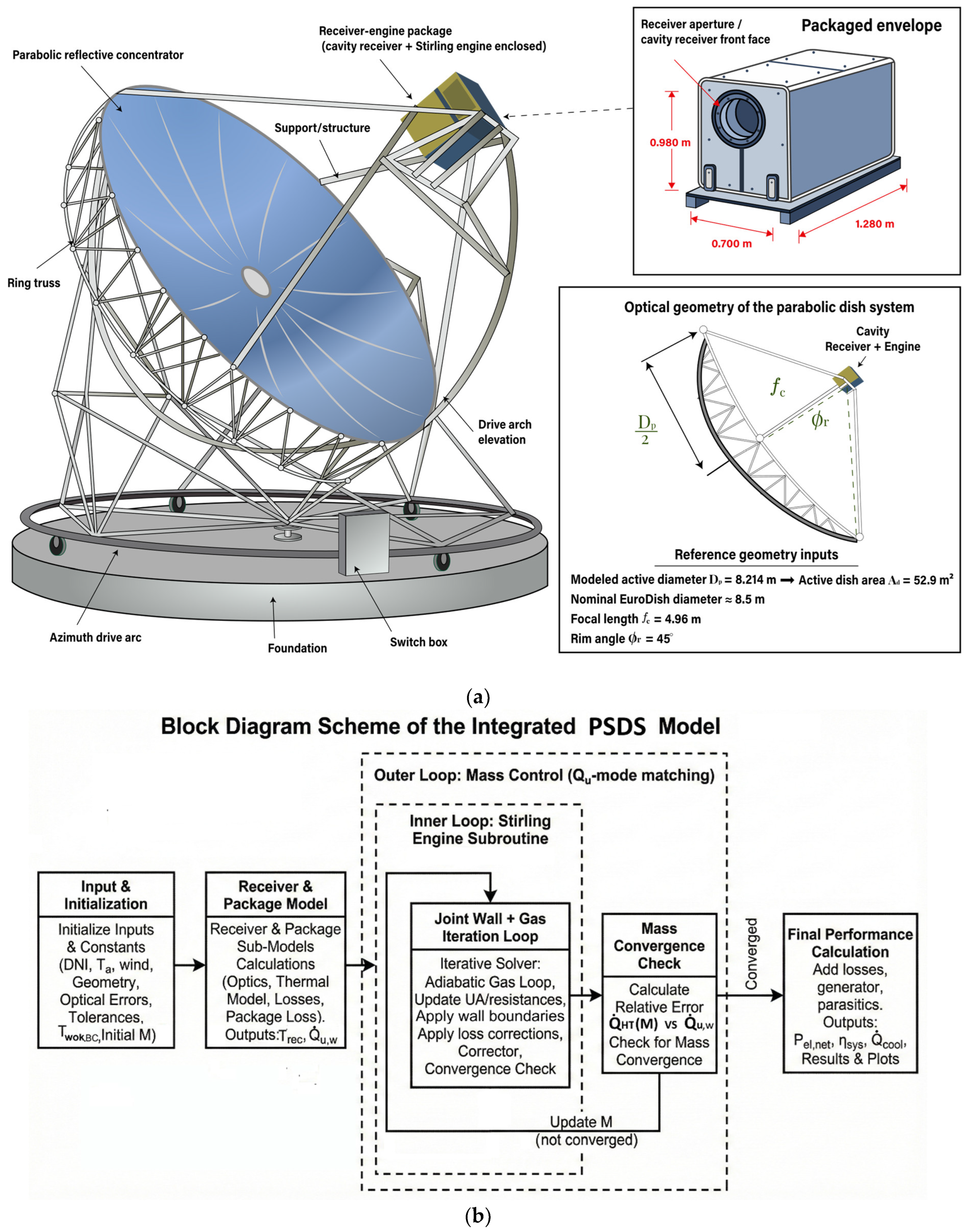
The physical layout of a representative dish–Stirling unit and the corresponding subsystem architecture of the integrated PSDS framework are summarized in Figure 1. The schematic in Figure 1a uses the EuroDish/SOLO-161 (SOLO Kleinmotoren GmbH, Sindelfingen, Germany) configuration as the reference example to indicate the main physical components, layout, scale, and principal geometry inputs. The indicated geometric quantities and package envelope dimensions are consistent with the EuroDish/SOLO-161 literature and the input set summarized in Appendix C [5,10,27].

Following are the definitions used in the model:

The incident solar power on the dish aperture is defined as:

$${\dot{\mathrm{Q}}}_{\mathrm{s}\mathrm{u}\mathrm{n}}=\mathrm{DNI} {\mathrm{A}}_{\mathrm{d}}\cos \left({\mathsf{\theta }}_{\mathrm{i}}\right),$$

(1)

where $A_{\mathrm{d}}$ is the active dish aperture area and ${\theta }_i$ is the incidence angle. In the EuroDish validation driver used here, ideal tracking is imposed and $\cos \left({\theta }_i\right)=1$. The absorbed receiver-side power is then as follows:

$${\dot{Q}}_{\mathrm{a}\mathrm{b}\mathrm{s}}={\eta }_{\mathrm{c}\mathrm{o}\mathrm{n}\mathrm{c}} \mathrm{D}\mathrm{N}\mathrm{I} A_d,$$

(2)

where ${\eta }_{\mathrm{c}\mathrm{o}\mathrm{n}\mathrm{c}}$ is the concentrator optical efficiency derived from the optical framework [17,28]. At the full-system level, the net electrical output is as follows:

$${ P}_{\mathrm{el-net}}={\mathsf{\eta }}_G{P}_{\mathrm{br}}-P_{\mathrm{par}},$$

(3)

where $P_{\mathrm{par}}$ is the parasitic consumption and the corresponding solar-to-electric efficiency is

$${\mathsf{\eta }}_{\mathrm{sys}}={\displaystyle \frac{P_{\mathrm{el-net}}}{{\dot{Q}}_{\mathrm{sun}}}}.$$

(4)

In this work, the dish/receiver/package description is developed up to the point where it provides the hot-side boundary quantities $T_{\mathrm{rec}}$ and ${\dot{Q}}_{\mathit{u.net}}$ to the Stirling engine submodel.

2.2. Dish–Receiver Front-End Model

2.2.1. EuroDish Reference Geometry and Optical Input

The dish/receiver front-end was built on the Mendoza et al. [17] dish/Stirling framework, but was suited to a fixed EuroDish-type geometry rather than a generic family of concentrators. In the implementation used here, the prescribed reference geometry is $D_p=8.214 \mathrm{m},$ rim angle ${\phi }_r=45°,$ receiver diameter $D_r=0.272 \mathrm{m},$ design geometric concentration $C_{G,D}=2526$ calculated in Equation (A17) (Appendix B), and receiver inclination $\beta =21°$ (facing downward) [5,10]. The radiative/optical material properties follow the EuroDish receiver assumptions used in the validation literature: mirror reflectivity ${\rho }_m=0.925$, receiver absorptivity ${\alpha }_{\mathrm{r}\mathrm{e}\mathrm{c}}=0.93$, receiver emissivity ${\epsilon }_{\mathrm{r}\mathrm{e}\mathrm{c}}=0.889$, cavity/insulation absorptivity ${\alpha }_{\mathrm{c}\mathrm{a}\mathrm{v}}=0.20$, and cavity/insulation emissivity ${\epsilon }_{\mathrm{c}\mathrm{a}\mathrm{v}}=0.90$ [5].

The optical efficiency is written in the form [17]

$${\mathsf{\eta }}_{\mathrm{conc}}={\mathsf{\rho }}_m\left(\cos {\mathsf{\theta }}_i\right)f_{s}G,$$

(5)

where ${\mathsf{\theta }}_i$ is the incidence angle, $G$ is the intercept factor and $f_s$ is the shading factor. In the EuroDish validation implementation, the product $f_{s}G$ (Appendix B) is constrained to reproduce the EuroDish reference optical input at the validation point, i.e.,

$${\mathrm{f}}_{\mathrm{s}}\mathrm{G}\approx 0.85,$$

(6)

while the underlying relations for interception, shading, and geometric concentration are retained as the formal optical framework of the model [17]. Thus, the present receiver front-end preserves [17] the structure but anchors the final absorbed power to the EuroDish reference optical chain. No additional glazing term is introduced in the final implementation, i.e., $\left(\tau \alpha \right)=1$ at the front-end level, consistent with the open cavity receiver configuration considered by Mendoza et al. [17]. Therefore, the receiver absorptance enters through ${\alpha }_{rec}$ and through the effective cavity absorptance formulation, defined below.

The active dish area is as follows:

$${ A}_d={\displaystyle \frac{\mathsf{\pi }{D}_p^2}{4}}$$

(7)

and the absorbed optical power is as follows:

$${\dot{Q}}_{abs}={\mathsf{\eta }}_{\mathrm{conc}}DNI{A}_d.$$

(8)

2.2.2. Receiver Wall Temperature Equilibrium Boundary

The receiver wall temperature provides the hot-side thermal boundary condition for the downstream engine model. This receiver-side boundary is computed using the closed-form receiver equilibrium relation adopted from Mendoza et al. [17]:

$$T_{\mathrm{rec}}={\left({\displaystyle \frac{DNI C_{G,D} {\mathsf{\alpha }}_{\mathrm{rec}}}{\mathsf{\sigma }{\mathsf{\epsilon }}_{\mathrm{rec}}}}\right)}^{1/4}{K}_{\mathrm{att}},$$

(9)

where $\sigma$ is the Stefan–Boltzmann constant and $K_{\mathrm{att}}$ is an attenuation constant. Following the Mendoza et al. [17] framework,

$$K_{\mathrm{att}}={\mathsf{\eta }}_{\mathrm{conc}}{F}_d{R}_{\mathrm{ref}},$$

(10)

with $F_d$ a deterioration factor and $R_{\mathrm{ref}}$ an effective cooling factor.

This point is one of the main modifications relative to Mendoza et al. In the original Mendoza/NEST formulation, $R_{\mathrm{ref}}$ appears as a generic cooling factor inside the attenuation constant. In the present PSDS model, $R_{\mathrm{ref}}$ is interpreted as an effective receiver cooling parameter that preserves the compact [17] temperature boundary but is subsequently used in a way that remains consistent with the coupled receiver engine heat balance. For engine-only parameter studies, $R_{\mathrm{ref}}$ is held fixed at the validated EuroDish value. For off-design receiver/environment perturbations, the attenuation/cooling representation can be re-identified so that the net receiver heat remains consistent with the downstream engine heat uptake.

2.3. Receiver Useful Heat and Coupling to the Engine Boundary

Before the explicit package loss channel is applied, the receiver-side useful heat delivered by the cavity model is defined as

$${ \dot{Q}}_{u,\mathrm{rec}}={\dot{Q}}_{\mathrm{abs}}-\left({\dot{Q}}_{\mathrm{rad},\mathrm{emi}}+{\dot{Q}}_{\mathrm{rad},\mathrm{ref}}+{\dot{Q}}_{\mathrm{conv},\mathrm{ap}}\right),$$

(11)

where ${\dot{Q}}_{\mathrm{rad},\mathrm{emi}}$ is the emitted radiative loss through the aperture, ${\dot{Q}}_{\mathrm{rad},\mathrm{ref}}$ is the reflected radiative loss through the aperture, and ${\dot{Q}}_{\mathrm{conv},\mathrm{ap}}$ is the aperture convection loss. A separate conductive receiver wall term is not treated as an independent loss channel in Module A; instead, the receiver-to-package thermal leakage is represented explicitly in Module B through the package loss (${\dot{Q}}_{\mathrm{pkg},\mathrm{total}})$ network described in Section 2.5.

The net heat passed to the engine boundary is, therefore,

$${ \dot{Q}}_{u,\mathrm{net}}={\dot{Q}}_{u,\mathrm{rec}}-{\dot{Q}}_{\mathrm{pkg},\mathrm{total}}.$$

(12)

The coupled receiver engine operating point is defined by the heat-matching condition

$${ \dot{Q}}_{u,\mathrm{net}}={\dot{Q}}_{\mathrm{heater}},$$

(13)

where ${\dot{Q}}_{\mathrm{heater}}$ is the heater heat uptake predicted by the Stirling engine model. This is the quantity that the variable charge control (Qu-mode) iteration ultimately enforces when the engine module is coupled to the receiver/package front-end.

2.4. Aperture Radiation, Reflection, and Convection Losses

2.4.1. Reflected and Emitted Radiation Through the Aperture

The receiver radiation treatment follows Mendoza et al. [17] loss decomposition into emitted and reflected components:

$${\dot{Q}}_{\mathrm{rad}}={\dot{Q}}_{\mathrm{rad},\mathrm{emi}}+{\dot{Q}}_{\mathrm{rad},\mathrm{ref}.}$$

(14)

The reflected term is retained in the form [17]

$${\dot{Q}}_{\mathrm{rad},\mathrm{ref}}=\left(1-a_{\mathrm{eff}}\right){\dot{Q}}_{\mathrm{abs}},$$

(15)

The effective cavity absorptance that governs the absorbed/reflected radiation partition is

$${ a}_{\mathrm{eff}}={\displaystyle \frac{{\mathsf{\alpha }}_{\mathrm{rec}}}{{\mathsf{\alpha }}_{\mathrm{rec}}+\left(1-{\mathsf{\alpha }}_{\mathrm{rec}}\right)\left(A_{\mathrm{rec}}/A_{\mathrm{cav}}\right)}}.$$

(16)

The emitted term is one of the principal modifications introduced in the present receiver submodel. Rather than using the single lumped emitting surface formulation of Mendoza et al. [17], the emitted aperture loss is evaluated as a view-factor-weighted [5,18] contribution from both the receiver and the internal cavity/insulation surfaces:

$${\dot{Q}}_{\mathrm{rad},\mathrm{emi}}=\mathsf{\sigma }\left({\mathsf{\epsilon }}_{\mathrm{rec}}{A}_{\mathrm{rec}}{F}_{\mathrm{rec}\to \mathrm{ap}}+{\mathsf{\epsilon }}_{\mathrm{cav}}{A}_{\mathrm{cav}}{F}_{\mathrm{cav}\to \mathrm{ap}}\right)\left(T_{\mathrm{rec}}^4-T_a^4\right),$$

(17)

where $F_{\mathrm{rec}\to \mathrm{ap}}$ and $F_{\mathrm{cav}\to \mathrm{ap}}$ are the numerical aperture view factors from the receiver and cavity surfaces to the aperture, respectively, calculated from the fixed cavity geometry using Equations (A21) and (A22) in Appendix B. These geometry-calculated factors are carried unchanged in the EuroDish validation cases. The emitted term therefore replaces the single lumped emitting surface formulation with an aperture emission estimate that separately weights the receiver and internal cavity/insulation surfaces. This treatment preserves direct comparability with the EuroDish radiation loss taxonomy reported by Reinalter et al. [5], while the reflected component retains the compact Mendoza effective absorptance form. In that mapping, ${\dot{Q}}_{\mathrm{rad},\mathrm{emi}}$ corresponds to the emitted radiation loss and ${\dot{Q}}_{\mathrm{rad},\mathrm{ref}}$ corresponds to the reflection term.

2.4.2. Convection Through the Aperture

The convection loss through the cavity opening is modeled as follows [29,30,31]:

$${\dot{Q}}_{conv,ap}=\left(h_{\mathrm{nat}}+h_{\mathrm{wind}}\right){ A}_{\mathrm{cav}}\left(T_{\mathrm{rec}}-T_a\right),$$

(18)

where $h_{\mathrm{nat}}, h_{\mathrm{wind}}$ are the natural and forced convective heat transfer coefficients respectively. The natural convection coefficient is written as

$${ h}_{\mathrm{nat}}={\displaystyle \frac{N{u}_{\mathrm{nat}}{k}_{\mathit{a.rec}}}{D_r}}.$$

(19)

Here, $k_{\mathit{a.rec}}$ is the thermal conductivity of the receiver and $N{u}_{\mathrm{n}\mathrm{a}\mathrm{t}}$ is the Nusselt number [17] (Appendix B). The wind-driven contribution retains functional dependence on receiver inclination [17],

$${ h}_{\mathrm{wind}}=f\left(\mathsf{\beta }\right)v_{\mathrm{wind}}^{n_w},$$

(20)

where $n_w$ is the wind exponent and the inclination function $f\left(\beta \right)$ is presented in Equation (A20) (Appendix B). Another explicit modification relative to the Mendoza receiver implementation is the wind speed exponent used in the forced-convection term. Mendoza et al. use the same general inclination-dependent structure but apply $n_w=1.104$ in their receiver model [17]. In the final EuroDish PSDS implementation, $n_w=1.401$ is used, following the experimentally derived cavity receiver wind correlation of R.Y.Ma [32], which expresses the head-on wind contribution as ${ h}_{forced}=f\left(\mathsf{\theta }\right)v^{1.401}$. The same exponent has also been adopted in later dish/Stirling hybrid system modeling [9]. Ma’s experiments showed that cavity receiver convective losses can increase strongly with wind and may reach approximately two to three times the no-wind convective level at high wind speed. The present implementation therefore retains the Mendoza-type inclination function and receiver loss structure while using an experimentally supported cavity receiver wind sensitivity in the final coupled PSDS simulations. Because Ma’s correlation was obtained for a specific cavity receiver and wind direction set, it is used here as an engineering receiver loss closure rather than as a universal forced-convection law. For validation against EuroDish, the receiver inclination is fixed at 21° facing downward, consistent with the measured receiver orientation used by Reinalter et al. [5].

2.5. Hot-End Package Loss Model

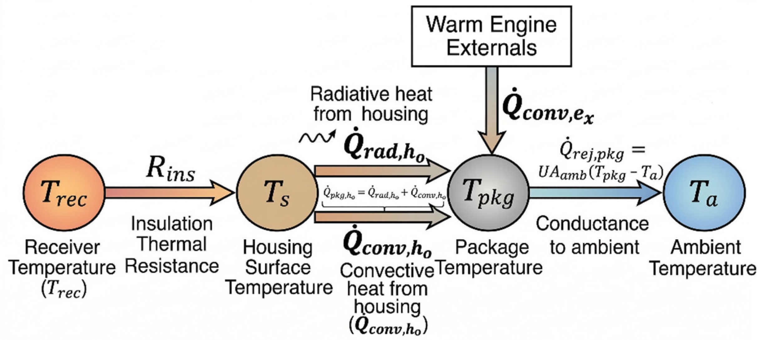
Reinalter et al. [5] identified an additional EuroDish loss channel as “radiation and convection into the STIRLING package”, i.e., heat transferred from the hot receiver housing and warm engine externals into the insulated engine package before final rejection to ambient. In the present work, this channel is retained explicitly as Module B and modeled as a lumped thermal network coupled to the predicted receiver temperature. The package loss representation adopted in the present work is illustrated schematically in Figure 2. The receiver-to-package heat transfer path is written as

$${ \dot{Q}}_{\mathrm{pkg},h_o}={\dot{Q}}_{\mathrm{rad},h_o}+{\dot{Q}}_{\mathrm{conv},h_o}={\displaystyle \frac{T_{\mathrm{rec}}-T_s}{R_{\mathrm{ins}}}},$$

(21)

where $T_s$ is the effective housing surface temperature and $R_{\mathrm{ins}}$ is an effective thermal insulation resistance between the receiver hot boundary and the housing surface. The housing contribution is decomposed into radiative and convective exchange with the package air:

$${\dot{Q}}_{\mathrm{rad},h_o}={\mathsf{\epsilon }}_h\mathsf{\sigma }{A}_{h_o}\left(T_s^4-T_{\mathrm{pkg}}^4\right), { \dot{Q}}_{\mathrm{conv},h_o}=h_{\mathrm{gap}}{A}_{h_o}\left(T_s-T_{\mathrm{pkg}}\right),$$

(22)

where ${ \epsilon }_h$, $A_{h_o}$, and $h_{\mathrm{gap}}$ are the effective housing emissivity, housing area, and internal package heat transfer convection coefficient, respectively, and $T_{pkg}$ is the package temperature. The total package heat load is

$${\dot{Q}}_{\mathrm{pkg},total}={\dot{Q}}_{\mathrm{pkg},h_o}+{\dot{Q}}_{\mathrm{conv},e_x},$$

(23)

where ${\dot{Q}}_{\mathrm{conv},e_x}$ accounts for heat transfer from the warm engine external surfaces. For off-design simulations, the package air temperature is coupled to ambient through an external rejection conductance:

$${\dot{Q}}_{\mathrm{pkg},\mathrm{total}}=U{A}_{\mathrm{amb}}\left(T_{\mathrm{pkg}}-T_a\right).$$

(24)

Only two effective parameters, $h_{\mathrm{gap} }$ and ${ R}_{\mathrm{ins}}$, are calibrated once at the EuroDish reference operating point to reproduce the package loss magnitude and split reported by Reinalter et al. [5] while maintaining positive, physically plausible values. The warm engine term ${\dot{Q}}_{\mathrm{conv},e_x}$ is retained separately, so that the package channel remains explicit and can be subtracted from the receiver useful heat before the receiver engine matching step. This treatment preserves the EuroDish loss accounting while avoiding over-parameterization of a loss channel that is only partially observable experimentally.

2.6. Receiver Engine Thermal Interface and Off-Design Identification of $R_{\mathrm{ref},\mathrm{eff}}\left(T_a,v_{wind}\right)$

The receiver/package front-end supplies two thermal boundary quantities to the Stirling engine model: the receiver wall temperature $T_{\mathrm{rec}}$ and the net useful heat rate available ${\dot{Q}}_{u,\mathrm{n}\mathrm{e}\mathrm{t}}$ after package losses. These are the hot-side boundary condition and the heat input constraint, respectively, used to drive the subsequent Stirling engine calculation. In the complete PSDS model, the engine returns the heater heat uptake ${ \dot{Q}}_{\mathrm{heater}}$, cooler rejection, shaft power, and electrical output, and the final operating point is obtained by enforcing

$${ \dot{Q}}_{\mathrm{heater}}={\dot{Q}}_{u,\mathrm{net}}$$

(25)

through the Qu-mode iteration on the working gas charge/mean pressure.

After the package loss network is evaluated, the net heat available at the Stirling engine boundary is defined as

$${\dot{Q}}_{u,\mathrm{net}}\left(T_{\mathrm{rec}},T_a,v_{wind}\right)={\dot{Q}}_u\left(T_{\mathrm{rec}},T_a,v_{wind}\right)-{\dot{Q}}_{\mathrm{pkg}}\left(T_{\mathrm{rec}},T_a,v_{wind}\right).$$

(26)

For off-design ambient wind operating points $\left({\mathrm{T}}_{\mathrm{a}},v_{\mathrm{wind}}\right),$ an effective receiver attenuation/cooling factor $R_{\mathrm{ref},\mathrm{eff}}\left(T_a,v_{wind}\right)$ is identified by enforcing consistency between the dish receiver useful heat and the engine heat uptake:

$${ \dot{Q}}_{\mathrm{heater}}\left(T_{\mathrm{rec}}\right)={\dot{Q}}_{u,\mathrm{net}}\left(T_{\mathrm{rec}},T_a,v_{wind}\right).$$

(27)

Here, ${\dot{Q}}_{\mathrm{heater}}$ is the heater heat uptake predicted by the non-ideal Stirling engine mode. In the coupled formulation, the engine-side heat uptake can be expressed approximately through the hot-side wall temperature drop across the heater tube wall:

$${\dot{Q}}_{heater}\approx {\displaystyle \frac{T_{\mathrm{rec}}-T_{wh}}{R_{ci,h}}} ,$$

(28)

where $T_{wh}$ is the heater inner wall temperature and ${ R}_{ci,h}$ is the hot-side tube wall conduction resistance:

$$R_{ci,h}={\displaystyle \frac{\ln \left(d_{ho}/d_{hi}\right)}{2\mathsf{\pi }{k}_{wh}{l}_h{N}_h}} ,$$

(29)

with $d_{hi}$ and $d_{ho}$ the heater tube inner and outer diameters, $k_{wh}$ the heater wall thermal conductivity, $l_h$ the heater tube length, and $N_h$ the number of heater tubes. This relation is consistent with the resistance-based hot-side heat transfer formulation used in the Stirling engine heat exchanger submodel.

The re-identification of $R_{\mathrm{ref},\mathrm{eff}}\left(T_a,v_{wind}\right)$ is applied only for off-design environmental perturbations that directly modify receiver heat losses, primarily through wind-driven convection, ambient-dependent radiative exchange, and package-to-ambient coupling. For parameter sweeps that act only on the engine side, such as speed, imposed cold-side boundary, etc., the external receiver cooling environment is unchanged and $R_{\mathrm{ref} }$ is, therefore, held fixed at its calibrated reference value. The resultant $R_{\mathrm{ref},\mathrm{eff}}\left(T_a,v_{wind}\right)$ is then used in the final variable charge (Qu-mode) system simulations to compute the coupled operating point and the net electrical output over the full $\left({\mathrm{T}}_{\mathrm{a}},v_{\mathrm{wind}}\right),$ operating space, without altering the underlying receiver energy balance structure inherited from the Mendoza front-end.

2.7. Non-Ideal Adiabatic Stirling Engine Model

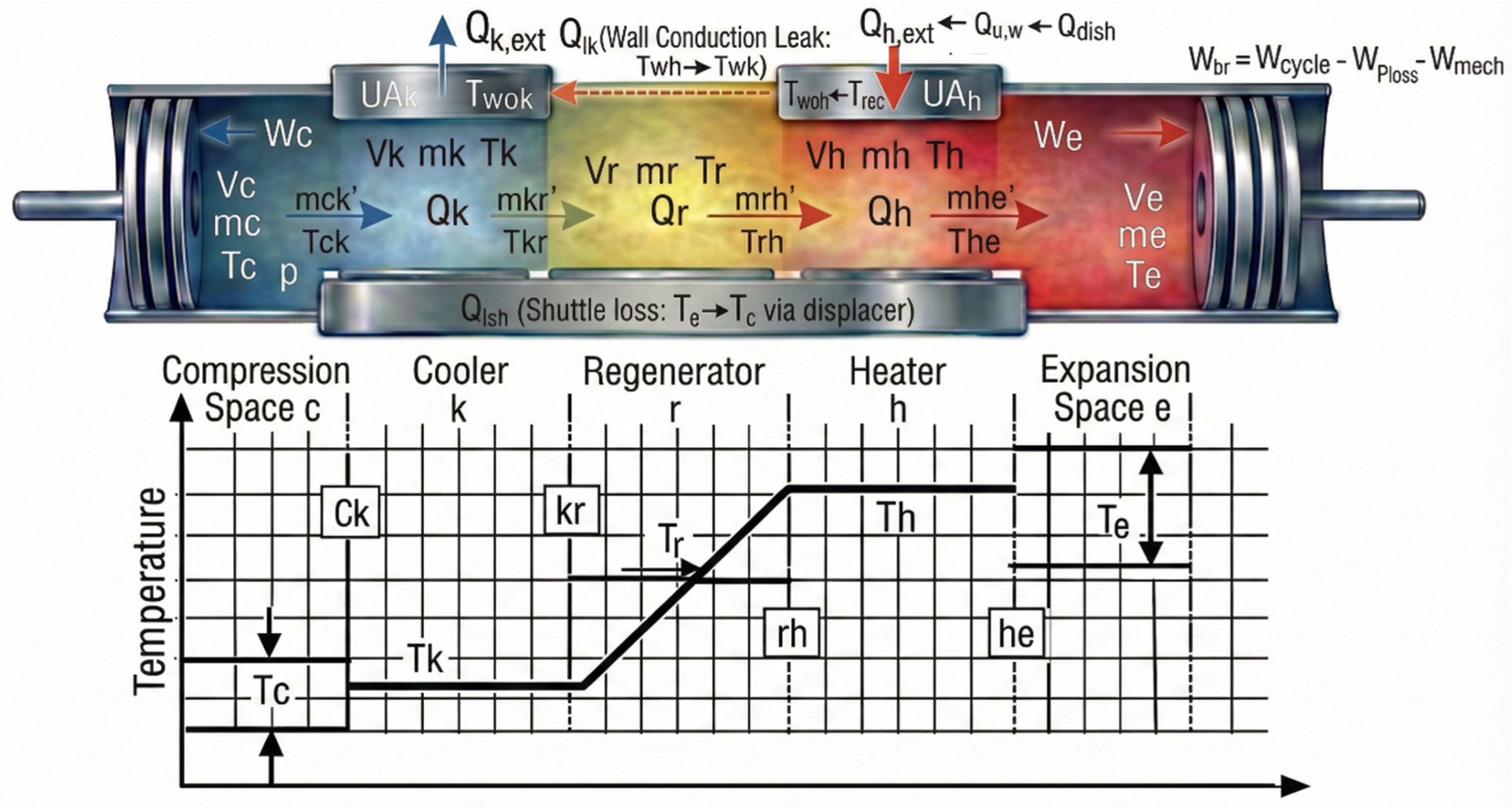
A second-order, non-ideal adiabatic Stirling engine model, shown schematically in Figure 3, is implemented using the control volume formulation of Araoz et al. [21] and classic adiabatic analysis (e.g., Urieli and Berchowitz [19]).

The working space is divided into five lumped control volumes: compression space (c), cooler (k), regenerator (r), heater (h), and expansion space (e). A single instantaneous pressure $p\left(\mathsf{\theta }\right)$ is assumed throughout the working gas, while the control volume masses evolve with crank angle $\mathsf{\theta }$.

2.7.1. Thermodynamic Enhancements to the Baseline Framework

While the proposed Non-ideal Stirling Engine (NI-SE) submodel leverages the foundational second-order adiabatic equations presented by Araoz et al. [21], several critical enhancements were implemented to increase the thermodynamic fidelity of the model and enable dynamic system-level integration.

Table 2. Principal enhancements introduced when adapting the Araoz non-ideal Stirling engine backbone to the coupled PSDS/EuroDish implementation.

Enhancement	Araoz et al. [21] 2014 Baseline/Modular Treatment	Present Implementation
Variable charge regulation for receiver engine heat matching	Engine solved at prescribed operating condition (e.g., mean pressure/frequency) within a modular standalone CHP-oriented framework	Working gas mass $m$ is iteratively adjusted so that the cycle-averaged heater requirement matches the useful heat available from the receiver/package front-end [4,10,27].
Explicit receiver/package thermal interface before the engine	External heat transfer module couples the engine to generic hot/cold sources, but no EuroDish receiver/package thermal front-end is included	Receiver/package model supplies $T_{\mathrm{r}\mathrm{e}\mathrm{c}}$ and ${\dot{Q}}_{u,\mathrm{n}\mathrm{e}\mathrm{t}}$ to the engine
Directional partitioning of regenerator losses within the coupled PSDS energy balance	Imperfect regeneration already included via $\epsilon$, $Q_{\mathrm{l}\mathrm{o}\mathrm{s}\mathrm{s},r}$, $Q_{ht}$, and $Q_{kt}$	Regenerator penalties are carried explicitly as heater- and cooler-side contributions inside the coupled operating point solution
Conductance update inside the receiver-coupled Qu-mode loop	Internal and external heat-transfer modules already exist and are iteratively solved	$U{A}_h$ and $U{A}_k$ are updated inside each mass-iteration of the coupled PSDS solution

distinguishes genuine system-level modifications relative to the Araoz et al. [21] engine framework from refinements that retain Araoz [21] non-ideal modular structure while adapting it to the coupled PSDS/EuroDish implementation. Further implementation-level refinements, including exchanger-wise cycle-resolved pumping loss evaluation, are described in Section 2.7.7.

2.7.2. Kinematics and Configuration

The thermodynamic core is configuration-agnostic; the machine type only affects the prescribed volume functions $V_c\left(\theta \right)$ and $V_e\left(\theta \right)$. The kinematic volume functions that drive the pressure volume work calculation are specified using an $\alpha$-type law [19,33]:

$$V_e\left(\theta \right)=V_{cle}+{\displaystyle \frac{V_{swe}}{2}}\left[1+\cos \left(\theta +\varphi \right)\right],$$

(30)

$$V_c\left(\theta \right)=V_{clc}+{\displaystyle \frac{V_{swc}}{2}}\left[1+\cos \left(\theta \right)\right],$$

(31)

$${\displaystyle \frac{{dV}_e}{\mathrm{d}\theta }}=-{\displaystyle \frac{V_{swe}}{2}}\sin \left(\theta +\varphi \right), {\displaystyle \frac{{dV}_c}{\mathrm{d}\theta }}=-{\displaystyle \frac{V_{swc}}{2}}sin\left(\theta \right),$$

(32)

where $V_{cle}$ and $V_{clc}$ are the expansion and compression space clearance volumes, $V_{swe}$ and $V_{swc}$ are the corresponding swept volumes, $\theta$ is the crank angle, and $\varphi$ is the phase angle, with $d{V}_e/d\theta$ and $d{V}_c/d\theta$ obtained analytically and used directly in the solver.

For $\beta , \gamma$ configurations, the same formulation applies by substituting the corresponding kinematic volume relations.

2.7.3. Uniform Pressure Ideal Gas Closure and Mass Partition

At each crank angle, the pressure follows the uniform pressure ideal gas constraint [21,34]:

$$p\left(\mathsf{\theta }\right)={\displaystyle \frac{mR}{\frac{V_c\left(\mathsf{\theta }\right)}{T_c\left(\mathsf{\theta }\right)}+\frac{V_k}{T_k}+\frac{V_r}{T_r}+\frac{V_h}{T_h}+\frac{V_e\left(\mathsf{\theta }\right)}{T_e\left(\mathsf{\theta }\right)}}} .$$

(33)

The fixed gas/dead volume terms of the heater, cooler, and regenerator are then defined as

$$V_h=N_{t,h}\mathsf{\pi }{\left({\displaystyle \frac{d_{i,h}}{2}}\right)}^2{l}_h, V_k=N_{t,k}\pi {\left({\displaystyle \frac{d_{i,k}}{2}}\right)}^2{l}_{c }, { V}_r=N_r\pi {\left({\displaystyle \frac{d_{i,r}}{2}}\right)}^2{l}_r,$$

(34)

where $V_h,V_k,{ V}_r$ are the heater, cooler, and regenerator gas volumes, respectively. The mass in each control volume is then written as

$$m_i\left(\mathsf{\theta }\right)={\displaystyle \frac{p\left(\mathsf{\theta }\right)V_i\left(\mathsf{\theta }\right)}{R{T}_i\left(\mathsf{\theta }\right)}}, i\in \{c,k,r,h,e\}.$$

(35)

The regenerator gas temperature is evaluated as a logarithmic mean between heater ($T_h)$ and cooler ($T_k)$ gas temperatures:

$$T_r={\displaystyle \frac{T_h-T_k}{\ln \left(T_h/T_k\right)}}.$$

(36)

2.7.4. Adiabatic State Update and Indicated Work

Compression- and expansion-space temperatures are advanced using the adiabatic open-system relations of [21,34,35], written in differential form as:

$${\displaystyle \frac{d{T}_c}{d\mathsf{\theta }}}=T_c\left({\displaystyle \frac{1}{p}}{\displaystyle \frac{dp}{d\mathsf{\theta }}}+{\displaystyle \frac{1}{V_c}}{\displaystyle \frac{d{V}_c}{d\mathsf{\theta }}}-{\displaystyle \frac{1}{m_c}}{\displaystyle \frac{d{m}_c}{d\mathsf{\theta }}}\right),$$

(37)

$${\displaystyle \frac{d{T}_e}{d\mathsf{\theta }}}=T_e\left({\displaystyle \frac{1}{p}}{\displaystyle \frac{dp}{d\mathsf{\theta }}}+{\displaystyle \frac{1}{V_e}}{\displaystyle \frac{d{V}_e}{d\mathsf{\theta }}}-{\displaystyle \frac{1}{m_e}}{\displaystyle \frac{d{m}_e}{d\mathsf{\theta }}}\right).$$

(38)

The indicated work ($W_{ind})$ and power ($P_{ind})$ are integrated over the cycle as:

$$W_{ind}=\oint p d{V}_c+\oint p d{V}_e, P_{ind}=W_{ind}/T_{cyc} ,$$

(39)

where the cycle period $T_{cyc}=1/f$ at frequency $f=RPM/60$.

2.7.5. Heater/Cooler Heat Transfer via Resistance-Based UA

Non-ideal heat transfer is modeled using effective conductances, consistent with the heater and cooler heat-transfer formulation of Araoz et al. [21]:

$${\dot{Q}}_h=U{A}_h\left(T_{woh}-T_h\right),\hspace{1em}{\dot{Q}}_k=U{A}_k\left(T_k-T_{wok}\right),$$

(40)

where $T_{woh}$ and $T_{wok}$ are the outer wall temperatures of the heater and cooler, respectively, with overall conductances:

$$U{A}_k={\left(R_{hi,k}+R_{ci,k}\right)}^{-1}, U{A}_h={\left(R_{hi,h}+R_{ci,h}\right)}^{-1}.$$

(41)

Here, $R_{hi}$ is the internal gas-side convection resistance and $R_{ci }$ is the tube wall conduction resistance. The internal coefficients $h_{ih}$ and $h_{ik}$ are updated from Reynolds-number correlations using the cycle mean pressure, so that the hot- and cold-side conductances are evaluated self-consistently within the wall/gas iteration. The detailed resistance expressions are given in Appendix A.

2.7.6. Regenerator Effectiveness and Loss Split

Regenerator imperfection is included using an NTU effectiveness relation [21,36]:

$${ϵ}_{reg}={\displaystyle \frac{NTU}{1+NTU}}, NTU=St\left({\displaystyle \frac{A_w}{A_c}}\right), {\displaystyle \frac{A_w}{A_c}}={\displaystyle \frac{4\left(1-ϵ\right)L}{{ϵ}_p{d}_w}},$$

(42)

where ${ϵ}_p$ is porosity, L is regenerator length, $dw$ is a wire/mesh diameter and St is the Stanton number (Appendix A). The regenerator convective heat term is split by flow direction and contributes to total heater and cooler duties through the following:

$${\dot{Q}}_{lossr,ht}=\left(1-{\mathsf{ϵ}}_{reg}\right){⟨\max \left({\dot{Q}}_{r,conv} ,0\right)⟩}_{cyc} ,$$

(43)

$${\dot{Q}}_{lossr,ck}=\left(1-{ϵ}_{reg}\right){⟨\min \left({\dot{Q}}_{r,conv} ,0\right)⟩}_{cyc} .$$

(44)

2.7.7. Pressure Drop, Pumping Loss, and Additional Non-Ideal Terms

Pressure losses in the heater, regenerator, and cooler are evaluated over the cycle using friction factor relations (Appendix A). The instantaneous pumping power is computed from the element pressure drop and the volumetric flow rate through the element, ${\dot{V}}_{flow,i}\left(t\right)={\displaystyle \frac{{\dot{m}}_l\left(t\right)}{{\rho }_i\left(t\right)}},$ giving the cycle pumping loss work:

$$W_{ploss}={\int }_{cyc}\sum _{i\in \{h,r,k\}}\Delta p_i\left(t\right){\dot{V}}_{flow,i}\left(t\right)dt.$$

(45)

While the commonly used pumping work form $\int \Delta p_i d{V}_e$ lumps all flow losses into an effective piston pressure difference [21,37], the present element-wise formulation evaluates the instantaneous dissipation $\Delta p_i\left(t\right){\dot{V}}_{flow,i}\left(t\right)$ in each exchanger, enabling component-resolved loss attribution and naturally handling flow reversals and local density variations. In the present PSDS implementation, this cycle-resolved pumping loss evaluation is retained explicitly inside the coupled operating point solution rather than treated only as a final aggregate correction. This ensures that exchanger-wise dissipation is propagated directly into the receiver engine energy balance and net-dispatch calculation.

Additional non-ideal heat-transfer terms include leakage and shuttle losses [37,38]:

$${\dot{Q}}_{lk}={\displaystyle \frac{K_r{A}_r}{L_r}}\left(T_{wh}-T_{wk}\right),$$

(46)

$${\dot{Q}}_{lsh}=0.4\left(T_e-T_c\right){\displaystyle \frac{z^2{K}_{\mathrm{pist}}{D}_d}{J_{\mathrm{pist}}{L}_d}},$$

(47)

where ${\dot{Q}}_{lk}$ represents an effective hot-to-cold conductive/leakage path, and ${\dot{Q}}_{lsh }$ represents shuttle heat transfer associated with reciprocating components; both are added to the system-level heater requirement and cooler rejection:

$${\dot{Q}}_{HT}={\dot{Q}}_h+{\dot{Q}}_{lossr,ht}+{\dot{Q}}_{lk}+{\dot{Q}}_{lsh},$$

(48)

$${\dot{Q}}_{cool}=\left|{\dot{Q}}_k+{\dot{Q}}_{lossr,ck}\right|+{\dot{Q}}_{lk}+{\dot{Q}}_{lsh}.$$

(49)

2.7.8. Brake Power and Net Electric Output

Brake work per cycle is computed as indicated work minus pumping and mechanical losses:

$${ P}_{ind}={\dot{Q}}_{HT}-{\dot{\mathrm{Q}}}_{cool},$$

(50)

$${ P}_{br}=P_{ind}-W_{ploss}-W_{mech}, { P}_{el-net}={\mathsf{\eta }}_G{P}_{br}-P_{cons},$$

(51)

where $W_{mech}$ is the cycle mechanical loss term obtained from a calibrated loss map as a function of cycle mean pressure and speed [39], ${\mathsf{\eta }}_G$ is generator efficiency and $P_{cons}$ is the constant auxiliary consumption.

2.7.9. Variable Charge (Mean Pressure) Control and Coupling (Qu-Mode)

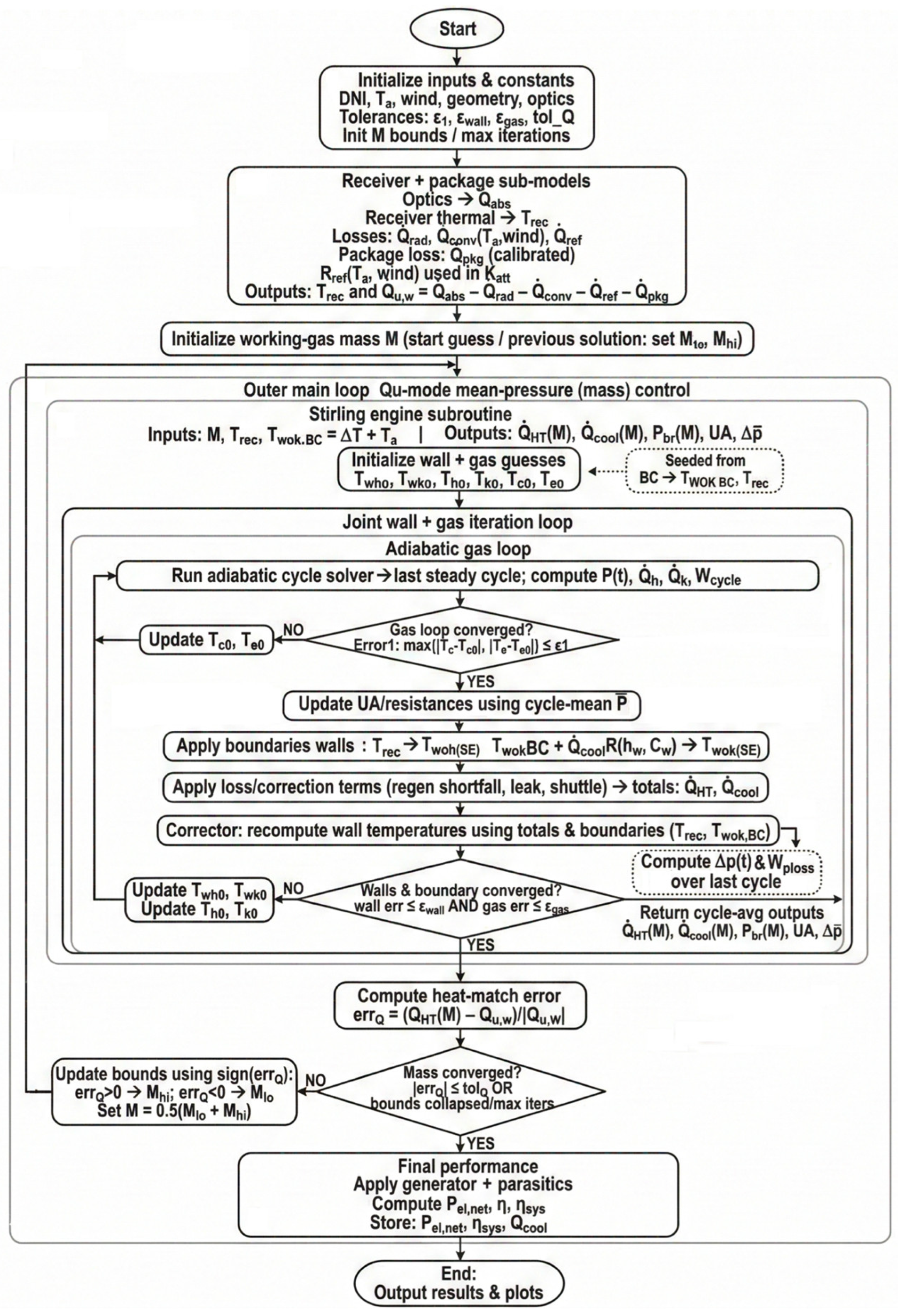
To couple the engine to the PSDS thermal front-end, the SE is operated under variable charge (mean pressure) control: the working gas mass $m$ (which directly governs the cycle-mean pressure $\overline{P}$) is iteratively adjusted so that the cycle-averaged total heater requirement ${\dot{Q}}_{HT}$ matches the useful heat available ${\dot{Q}}_{u,w}\equiv {\dot{Q}}_{u,\mathrm{n}\mathrm{e}\mathrm{t}}$ to the heater interface:

$${⟨{\dot{Q}}_{HT}\left(m\right)⟩}_{cyc}={\dot{Q}}_{u,w}, {\dot{Q}}_{u,w}=\max \left({\dot{Q}}_{u, dish}-{\dot{Q}}_{pkg},0\right).$$

(52)

A bisection update is applied on $m$ using the residual:

$$er{r}_Q\left(m\right)={⟨{\dot{Q}}_{HT}\left(m\right)⟩}_{cyc}-{\dot{Q}}_{u,w}$$

(53)

until $\left|er{r}_Q\right|/Q_{u,w}\le to{l}_Q$, where $\left(to{l}_Q\right)$ is the prescribed heat match tolerance. For each mass trial, an inner periodic cycle solver advances the adiabatic state equations, while a coupled wall/gas loop updates the convective heat transfer coefficients $h$, the overall thermal conductances ($U{A}_h, U{A}_k$), the wall temperatures $T_w$, and pressure drop losses from Reynolds numbers based on the cycle mean pressure. Consequently, the wall and gas states are converged self-consistently within each mass trial (Qu-mode), so that the final receiver-coupled operating point is obtained from a thermally consistent heat match condition rather than from a prescribed mean pressure engine solution. The numerical solution sequence used to converge each coupled operating point is summarized in Figure 4.

2.7.10. Cold-Side Boundary and External Cooling Path

The cold-side boundary imposed by the heat rejection system is prescribed through the cooling fluid inlet temperature, consistent with the external cooling fluid treatment of Araoz et al. [21], who use the inlet water temperature as the external cooler-side boundary and compute the cooler outer wall temperature from it.

For the EuroDish reference case, Nepveu et al. [10] report a water cooler temperature range of 295–305 K at an ambient temperature of $293 K,$ while Reinalter et al. [5] determine the cooling power from the coolant enthalpy rise between inlet and outlet, confirming that inlet and outlet coolant temperatures are distinct bulk quantities in the external cooling loop.

At the system level, fixed-approach reset strategies have also been used to relate cooling-water temperature to ambient sink conditions. For example, Liu and Chuah [40] define the approach temperature as the difference between ambient wet-bulb temperature and condensing water temperature and note that earlier fixed approach strategies used ambient wet-bulb temperature alone to reset the condensing water temperature. By analogy with such fixed approach system-level controls, the present reduced order PSDS implementation approximates the inlet coolant boundary from the selected ambient sink temperature by

$$T_{coolant,in}\equiv T_{wok,BC}=T_a+\Delta T_{app},$$

(54)

where $\Delta T_{app}$ is the imposed approach temperature between ambient and the cooler-side external boundary; in the present implementation, water is used as the coolant fluid.

This ambient-plus-approach relation is adopted here as a reduced order system-level closure for the external cooling loop.

For a rejected heat rate ${\dot{Q}}_{cool}$, the bulk-to-wall rise across the external cooling path is written as follows:

$$T_{wok}=T_{wok,BC}+{\dot{Q}}_{cool}\left({\displaystyle \frac{1}{h_{ok}{A}_c}}+{\displaystyle \frac{1}{2{\dot{m}}_{cool}{c}_{p,cool}}}\right),$$

(55)

where $T_{wok}$ is the cooler outer wall temperature, $h_{ok}$ is the external heat transfer coefficient, ${\dot{m}}_{cool}$ is the coolant mass flow rate, and $c_{p,cool}$ is the coolant specific heat. This relation is consistent with the external cooler wall treatment of [21]:

$$T_{coolant,out}=T_{wok,BC}+{\displaystyle \frac{{\dot{Q}}_{cool}}{{\dot{m}}_{cool}{c}_{p,cool}}} .$$

(56)

This is followed by tube wall conduction and internal convection to obtain $T_{wk}$ and the cooler gas temperature $T_k$ (Appendix A).

Distinct from standalone engine studies, the present implementation is embedded in a PSDS system model: the heater-side heat input is constrained by receiver/package useful heat ${\dot{Q}}_{u,w}$ via variable charge control, while the cold-side boundary is imposed through ambient-driven heat rejection. This enables fully coupled performance sweeps over DNI and environmental conditions.

2.7.11. EuroDish Reference Point Calibration and Parameter Hierarchy

Before formal validation, the coupled receiver/package/engine framework was anchored at the EuroDish reference operating point. At $DNI=906 W m^{-2}$, using the corresponding EuroDish ambient and cooling conditions reported by Nepveu et al. [10], the benchmark receiver engine heat-input closure was

$${\dot{Q}}_{u,net}={\dot{Q}}_{heater}\approx 31.63 \mathrm{kW}.$$

(57)

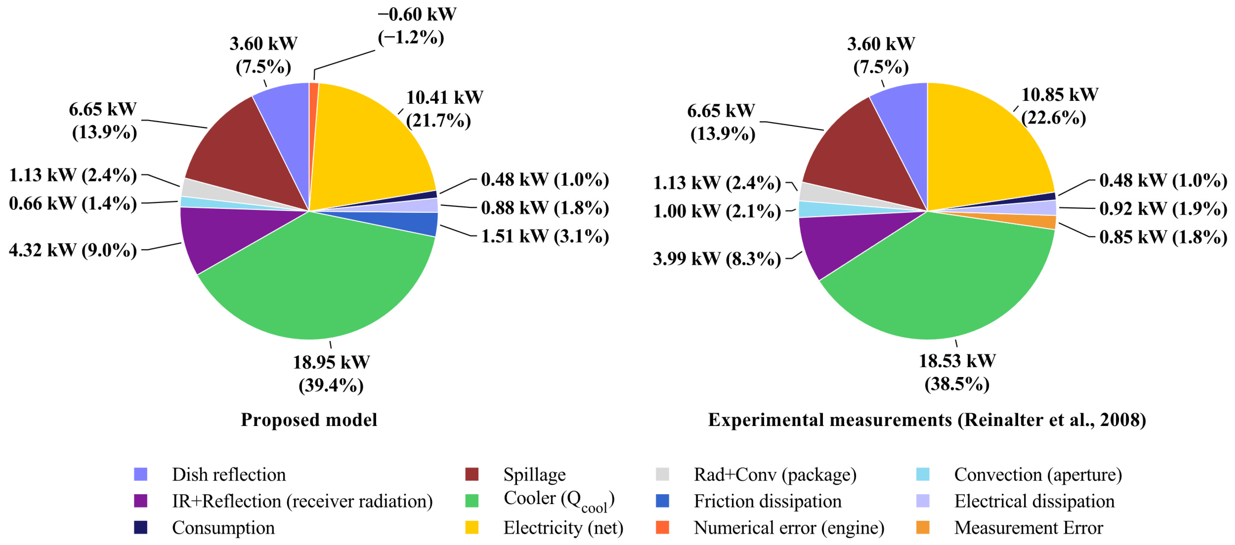
The package loss channel was anchored at the same reference point using ${\dot{Q}}_{pkg,total}\approx 1.13 \mathrm{kW}$, consistent with the EuroDish dispatch and loss partition benchmark reported by Reinalter et al. and Nepveu et al. [5,10].

This reference point anchoring yielded three effective calibrated quantities: the receiver attenuation/cooling factor ${ R}_{ref}$, and the two package loss parameters $h_{gap}$ and $R_{ins}$. The EuroDish geometry, optical/material properties, engine geometry, heat transfer and loss correlations, generator efficiency, parasitic load, and the optical product $f_{s}G$ were fixed before the integrated validation. The package-to-ambient conductance $U{A}_{amb}$ was then derived from the package heat rejection balance. After the reference calibration, $R_{ref}$, $h_{gap}$, $R_{ins}$, and $U{A}_{amb}$ were carried unchanged into the integrated EuroDish DNI validation and into the engine-side speed, heat exchanger, and cooling boundary sweeps.

For the environmental sweep in $\left(T_a,v_{wind}\right)$, the effective quantity $R_{ref,eff}\left(T_a,v_{wind}\right)$ is used as a receiver-side closure parameter for the changed ambient/wind receiver loss state. In that sweep, the package coefficients $h_{gap}$, $R_{ins}$, and $U{A}_{amb}$ retain their reference-calibrated values, while $R_{ref,eff }$ is identified through the receiver engine heat-matching condition in Equation (27). The heat match residual is controlled by the Qu-mode tolerance in Equation (53); with $to{l}_Q={10}^{-3}$, the numerical heat closure residual is bounded to approximately $0.1\%$ for the off-design environmental identification.

Table 3. Calibration hierarchy of the coupled EuroDish PSDS model. Numerical values are listed in Appendix C.

Quantity/Parameter Group	Treatment	Constraint/Definition	Application in the Study
EuroDish geometry, optical/material properties, Stirling engine geometry, heat transfer/loss correlations, generator efficiency, and parasitic load	Fixed inputs	Literature and benchmark definitions	All simulations
$f_{s}G$	Fixed optical anchor	EuroDish optical chain reference input	EuroDish receiver/front-end simulations
$R_{ref}$	One-point calibrated receiver parameter	Reference heat input closure ${\dot{Q}}_{u,net}\approx 31.63 \mathrm{kW}$ at $DNI=906 W{m}^{-2}$	EuroDish DNI validation and engine-side parametric sweeps
$h_{gap}$	One-point calibrated package parameter	Package = loss closure at ${\dot{Q}}_{pkg,total}\approx 1.13 \mathrm{kW}$ and ${\dot{Q}}_{conv,h,ref}$ the reference package loss split	Package model
$R_{ins}$	One-point calibrated package parameter	Package loss closure at ${\dot{Q}}_{pkg,total}\approx 1.13 \mathrm{kW}$ and ${\dot{Q}}_{rad,h,ref}$ the reference package loss split	Package model
$U{A}_{amb}$	Derived package parameter	Package-to-ambient heat rejection balance	Off-design package rejection
$R_{\mathit{ref},\mathit{eff}}\left(T_a,v_{\mathit{wind}}\right)$	Environmental receiver closure variable	Receiver engine heat-matching condition under ambient/wind perturbation	Ambient wind sweep only

summarizes the parameter hierarchy, and the corresponding numerical inputs are listed in Appendix C.

2.8. Verification and Validation Protocol/Setup

To establish credibility at three levels and to reduce the risk of compensating errors between submodels, a staged benchmarking strategy was adopted. This structure is appropriate because the proposed framework combines inherited receiver and engine backbones with receiver/package coupling, Qu-mode operating point treatment, and loss-channel refinements introduced in the present work. First, the Mendoza-based dish/receiver backbone was verified against the published receiver relations and reference cases of Mendoza et al. [17], including the closed-form receiver temperature expressions and the S1–S5 receiver cases. Second, the standalone non-ideal Stirling engine (NI-SE) submodel was validated against the GPU-3/LeRC benchmark used by Araoz et al. [21,39,41], so that the internal engine thermodynamics, heat transfer closures, conductance treatment, and loss calculations could be assessed under prescribed thermal boundary conditions independently of the solar receiver. Third, the fully coupled PSDS model was validated against EuroDish operating and dispatch data reported by Nepveu et al. and Reinalter et al. [5,10], thereby testing the complete receiver–package–engine–generator chain, including package losses, Qu-mode heat matching, generator conversion, and parasitic terms. Since the integrated validation compares engine heat input, cooler rejection, and net electrical output, model agreement is assessed across the propagated system energy balance rather than through a single terminal output. See Appendix C for the benchmark inputs and the full numerical input set used in the present work, including the baseline EuroDish reference parameters, calibrated receiver/package coefficients, standalone GPU-3/LeRC validation conditions, integrated EuroDish benchmark inputs, solver settings, transferability substitutions, and parametric sweep matrices.

2.8.1. Receiver Front-End Verification Against Mendoza et al. [17]

The receiver front-end verification was limited to the unmodified Mendoza receiver backbone. The verification targeted (i) the closed-form receiver temperature relations reported by Mendoza et al. [17] (Equations (9) and (10)), and (ii) the S1–S5 receiver cases summarized in their Table 7 [17]. Because the final PSDS receiver implementation introduces a view-factor-based emitted radiation term and a modified wind exponent, this stage is interpreted as an implementation check of the inherited Mendoza backbone, rather than as a validation of the final EuroDish-adapted receiver model. The Table 7 [17] benchmark was used mainly to check the consistency of the absorbed power and receiver loss partition produced by the receiver solver under the published S1–S5 geometries and efficiencies. In the implemented Mendoza verification, the common benchmark conditions were $DNI=1000 W{m}^{-2}$, $T_a=301 K$, and $v_{wind}=1.5 m{s}^{-1}$, together with the S1–S5 geometry cases and the Table 5 [17] optical factor settings used in the reproduced comparisons corresponding to Figure 10 and Table 7 of Mendoza et al. [17]; the full numerical values are listed in Appendix C.

2.8.2. Standalone NI-SE Validation Against GPU-3/LeRC

The NI-SE submodel was validated against the GPU-3 (General Motors, Detroit, MI, USA) benchmark adopted by Araoz et al. [21,39,41,42]. For this standalone validation, the external thermal boundary conditions were prescribed to reproduce the LeRC/GPU-3 test conditions, so that the internal cycle solution, heat transfer closures, and pressure drop/loss calculations could be assessed independently of the solar receiver. The benchmark covered operating frequencies from 16.7–58.3 Hz at $\overline{p}\approx 2.76 MPa$, a hot-side boundary temperature of ~704 °C, and a cooling water inlet temperature of ~15 °C, consistent with the GPU-3 comparisons reported by Araoz et al. [21,39,41].

2.8.3. Integrated PSDS Validation Against EuroDish

To validate the complete PSDS model against EuroDish operation data, the EuroDish benchmark state was taken primarily from the operating conditions reported by Nepveu et al. [10], including hydrogen as working gas, $DNI=906 W{m}^{-2}$, $solar energy=48 kW$, a water cooler temperature range 295–305 K, ambient temperature $293 K$ and engine speed $1500 rpm$. In the validation step, this integrated benchmark was simulated using the EuroDish/SOLO V161-type engine geometry and kinematics defined in Section 2.7 and Appendix C, consistent with the EuroDish configuration reported by Nepveu et al. [10]. The resultant receiver heat, cooler rejection, and electrical output were then compared against the EuroDish dispatch and power partition data reported by Nepveu et al. and Reinalter et al. [5,10]. This final stage tested the complete coupling between the receiver/package front-end, the Qu-mode engine solution, and the electrical output calculation.

2.9. Transferability Study Setup

To evaluate the cross-platform generalizability of the integrated PSDS framework, the model was re-parameterized using the comparative dish–Stirling specifications reported in Mancini Table 2 [4]. Four representative platforms were considered: SBP (SOLO-161 class Schlaich Bergermann Partner, Stuttgart, Germany), SES (Stirling Energy system, Phoenix, AZ, USA), WGA Mod 1 (ADDS, WGAssociates, Dallas, TX, USA), and SAIC/STM (Science Applications International Corp., Reston, VA, USA). For quantitative parity comparisons, the pressure-controlled systems SBP, SES, and WGA Mod 1 were simulated in the corresponding variable charge/mean pressure mode, while SAIC/STM was retained only as qualitative context because its variable-stroke control architecture is not explicitly represented in the present framework. No platform-specific recalibration was introduced; instead, the model was reassigned using the geometric and operating specifications reported in Mancini Table 2 [4]. These were used together with the standardized secondary assumptions listed in Appendix C—namely, the projected dish area, reflectivity, intercept factor where reported, receiver aperture diameter, peak concentration and/or focal length, engine displacement, working fluid, and nominal rotational speed [4].

Because the summary specifications in Mancini Table 2 [4] do not uniquely define balance-of-plant details or thermal boundary conditions, a small set of secondary inputs was standardized to enable a consistent portability test across platforms. Auxiliary consumption was represented by a constant parasitic term, $P_{cons}=P_{const}$. In the present portability implementation, $P_{const}$ was set to 4.8% of rated electrical power, obtained by scaling the EuroDish reference parasitic level of 0.48 kW relative to the nominal 10 kW system rating [5]; this was used as a standardized portability assumption rather than as a platform-specific measured quantity. Reinalter et al. are used only to anchor the EuroDish generator/parasitic reference context [5].

The engine cold-side boundary was standardized to $T_{wok,BC}=295 K$ [10] for all platforms, equivalently $T_{wok,BC}=T_{amb}+∆T_{app}$ under the Mancini normalization $T_{amb}=288 K$ [4]. Package losses were computed using the EuroDish/Reinalter-calibrated enclosure model and scaled by aperture area similarity, with the effective housing/package area scaled with receiver aperture size in the portability implementation [5]. Multi-cylinder engines were approximated by an equivalent number of identical alpha-type modules using displacement-based scaling. These standardized assumptions are not intended to reproduce each platform’s as-built balance of plant; rather, they isolate whether the coupled receiver engine formulation preserves physically consistent scaling and trend behavior across disparate system sizes and architectures.

Model outputs were benchmarked against Mancini’s reported peak net electrical power and peak net efficiency values, which are normalized to clean mirrors, $T_{amb}=288 K$, and $DNI=1000 W{m}^{-2}$ [4]. For SBP, the peak efficiency reference was taken at the reported design point condition of $DNI=800 W{m}^{-2}$, consistent with the note to Mancini Table 2 [4]. In addition to the peak points, the predicted $P_{el}\left(DNI\right)$ curves were compared against trend curves derived from Mancini’s [4] reported performance plots to assess consistency over the broader irradiance range.

Because system-specific receiver thermal loss coefficients and detailed cavity characterization are not fully defined in the Table 2 summary [4], the receiver submodel was operated using the Mendoza-type baseline cooling/attenuation [17] factor ${ R}_{ref}=0.5$, rather than a platform-specific fitted value. This quantity enters the attenuation term $K_{att}$ and maps the idealized equilibrium receiver temperature to realistic operating levels [5,10] in the Mendoza receiver formulation [17] (Equations (9) and (10)). A common baseline value $R_{ref}=0.5$ was, therefore, used across the transferability runs to avoid ad hoc tuning of receiver losses, while the EuroDish validation case retained its separately calibrated value $R_{ref}=0.579$. Remaining discrepancies between model predictions and the normalized Table 2 [4] peaks are expected, because the summary specifications do not uniquely determine several system-dependent contributors, including receiver thermal loss coefficients, parasitic loads, cooling system details, and proprietary control logic. The transferability study, therefore, tested whether the coupled receiver engine formulation preserves physically consistent scaling and trend behavior across systems of different size and architecture, and whether deviations can be traced primarily to known control/auxiliary differences rather than to deficiencies in the core model formulation.

2.10. Parametric Sensitivity Studies

The sensitivity studies referenced the EuroDish-calibrated model, with fixed geometry, package loss calibration, and control settings. For the comparative off-design studies, however, a nominal study baseline of ${ T}_a=288 \mathrm{K}$ was adopted, consistent with the ambient normalization used in comparative dish–Stirling performance reporting by Mancini et al. [4]. This nominal study baseline is, therefore, distinct from the EuroDish validation ambient of $293 \mathrm{K}$ used in Section 2.8.3. Unless otherwise stated, the comparative sweeps were conducted at $DNI=906 W{m}^{-2}$, $v_{wind}=1.5 m{s}^{-1}$, and ${ T}_{wok,BC}=295 \mathrm{K}$, with the latter retained from the validated EuroDish reference case [5,10]. This choice is consistent with the Stirling submodel structure, in which the cooler side external heat transfer module is driven by the inlet cooling fluid temperature to determine the cooler outer wall temperature and the cooling requirement [21] (Equations (54) and (55)). The exact discrete parameter levels used in each sweep are listed in Appendix C.

Receiver-to-engine coupling was enforced using variable charge (mean pressure) control (Qu-mode), in which the working gas charge is iterated until the cycle-averaged total heater heat requirement predicted by the Stirling model matches the net heat available from the front-end after package losses (Section 2.7.9). For engine-side parametric sweeps (RPM, heat exchanger sizing, and cold boundary), the receiver-side operating point was held fixed at the validated baseline (fixed $R_{ref}$ and fixed baseline $T_{rec}$ and ${\dot{Q}}_{avail}$), so that the resulting trends isolate engine internal thermofluid and mechanical penalties under Qu-mode control.

The following four parametric sweeps were conducted:

Engine speed sweep. The rotational speed was varied over $n=1000÷3500 rpm$ at fixed $DNI=906 W{m}^{-2},$ $T_{amb}=288 K,$ $v_{wind}=1.5 m{s}^{-1},$ and baseline receiver/package conditions (Appendix C). This sweep isolates speed-dependent internal penalties, primarily pressure drop/pumping losses and mechanical losses, and quantifies the resulting changes in $P_{\mathit{el-net}}$, ${\eta }_{br}$, ${\eta }_{sys}$, and cooler rejection.

Heat exchanger scaling sweep. A geometric scaling factor $s_L$ was applied to the heater and cooler tube lengths according to $l_h=s_L{l}_{h0}$ and $l_c=s_L{l}_{c0}$, while all other engine geometries were kept unchanged ($l_{h0},l_{c0}$ are listed in Appendix C). This scaling simultaneously modifies the internal heat transfer conductance, the heater/cooler dead volumes, (e.g., $v_h\propto l_h,v_k\propto l_c$), and the pressure drop losses (Darcy-type scaling $\Delta p\propto L$), and, therefore, quantifies the classical $UA$-dead-volume pressure drop trade-off and identifies regions of diminishing returns in net output. Near-optimal alternatives were identified by applying an optimal Modeling to Generate Alternatives (MGA)-based near-optimality criterion [43] to the heat exchanger scaling sweep, with designs within 2% ${(\mathsf{ϵ}}_{mga}=2\%,)$ of the maximum net electrical output retained as practically equivalent alternatives $({\mathit{i.e.},P}_{\mathit{el-net}}\ge \left(1-{ϵ}_{mga}\right)P_{el,max}).$

Environmental sweep $\left({\mathit{T}}_{\mathit{a}},\mathit{w}\mathit{i}\mathit{n}\mathit{d}\right)$. Ambient temperature and wind speed were varied over $v_{wind}=0÷10 m{s}^{-1},$ $T_{amb}=273.15 K÷313.15 K,$ at fixed $DNI=906 W{m}^{-2}$. This sweep evaluates robustness to ambient variability and re-identifies ${ R}_{ref,eff}\left(T_a,V_{wind}\right)$ through the receiver engine energy balance procedure of Section 2.6, after which the final system performance was evaluated in Qu-mode using the resulting $R_{ref,eff}$. Capability envelopes of net electrical power over the $\left(T_a,wind\right)$ domain were also evaluated for the heat exchanger scaling study; the full envelope results are reported in Supplementary Figure S1.

Cold boundary sweep (${\mathit{T}}_{\mathit{w}\mathit{o}\mathit{k},\mathit{B}\mathit{C}}$/$\mathsf{\Delta }{\mathit{T}}_{\mathit{a}\mathit{p}\mathit{p}}$). The cold-side boundary was swept by varying $\Delta T_{app}$ over $5÷25$ at $T_a=288 \mathrm{K}$ giving $T_{wok,BC}\equiv T_{coolant,in}=293÷313 K$ through Equation (54). This sweep was performed at DNI = 400, 600, and 906 $W{m}^{-2}$, with fixed $\mathrm{n}=1500 \mathrm{r}\mathrm{p}\mathrm{m}$ and $s_L=1.0(l_{h0},l_{c0})$. For each DNI case, the receiver/package front-end was held fixed at the baseline output vector corresponding to that irradiance level (Appendix C), while the Stirling engine submodel was re-solved in variable charge control (Qu-mode) for the imposed cooling boundary. The resultant changes in $P_{\mathit{el-net}}$, ${\dot{Q}}_{cool}$, and the remaining loss terms quantify the sensitivity of the system to attainable coolant inlet temperature and the redistribution of fixed thermal input between electrical output and rejected heat, which is relevant for downstream thermal utilization.

3. Results and Discussion

3.1. Receiver Front-End Verification Against Mendoza et al. [17]

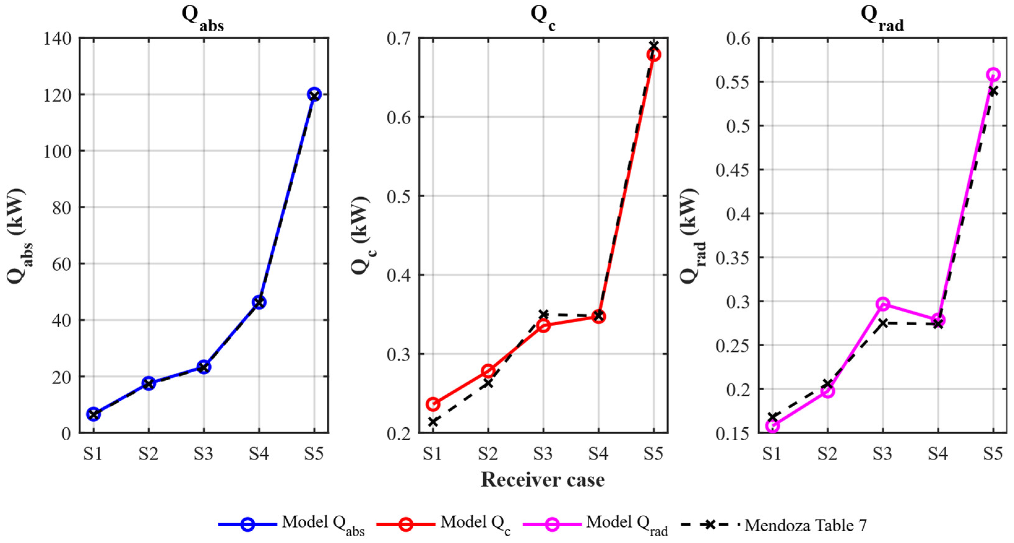
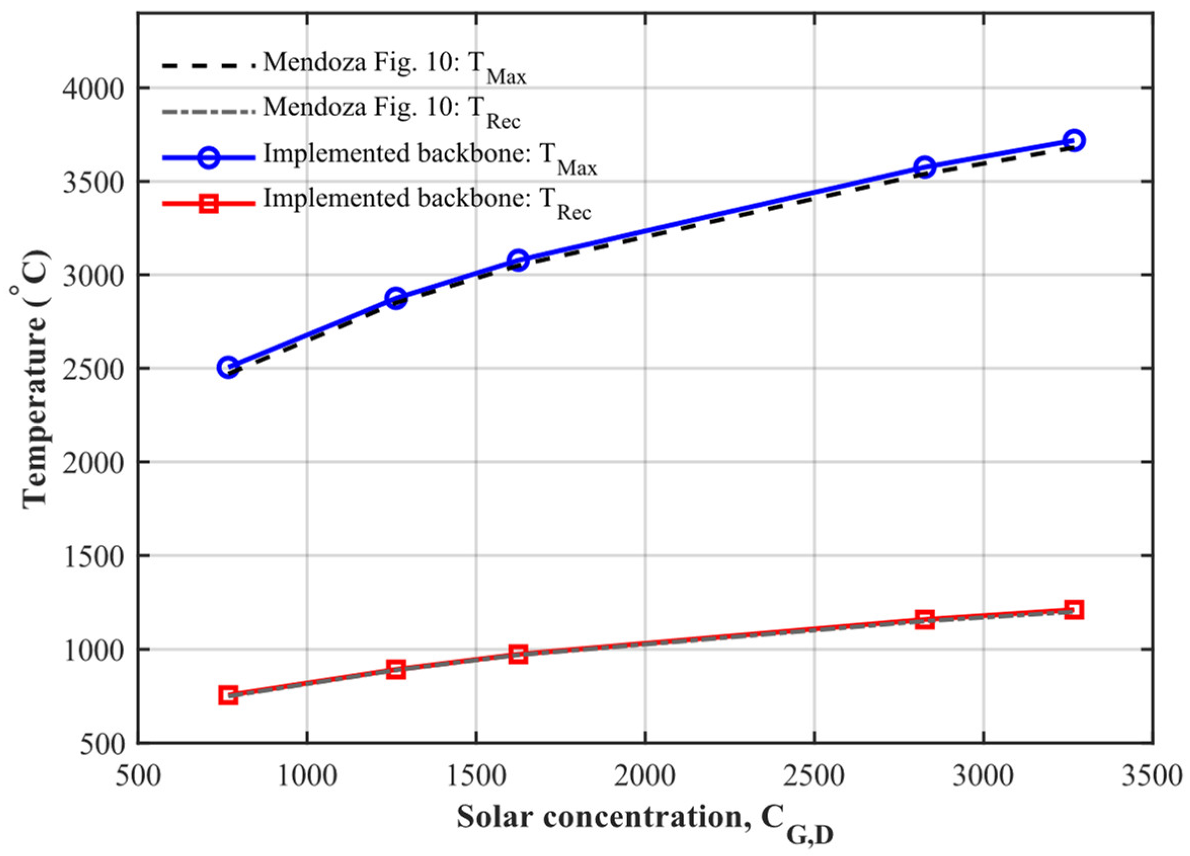
The Mendoza-based receiver backbone was first verified independently of the final EuroDish-specific modifications. Figure 5 compares the reproduced closed-form receiver-surface temperature relations with the corresponding benchmark curves reported by Mendoza et al. [17]. This check confirms that the present implementation reproduces the analytical receiver temperature boundary inherited from the Mendoza [17] formulation and, therefore, preserves the intended front-end backbone before the EuroDish-specific refinements are introduced.

A second receiver check was performed against the S1–S5 cases reported in Mendoza Table 7 [17]. In this benchmark, the published receiver efficiency was imposed in the energy balance closure. The comparison, therefore, serves as a consistency check of the optical absorption and receiver loss partition rather than as a fully independent predictive validation. The present implementation reproduced the absorbed optical power and preserved the expected balance between convection and radiation losses across the S1–S5 cases, confirming that the Mendoza [17] receiver equations were coded consistently and that the inherited backbone behaves correctly over the benchmark geometric range. The corresponding values are shown in Figure 6. Taken together, these receiver-side checks indicate that the present framework reproduces the inherited Mendoza [17] receiver formulation correctly. This is of import because the final PSDS front-end departs from the original Mendoza [17] model only after this backbone stage—namely, through the EuroDish-specific optical anchoring, the view-factor-based emitted radiation term, the modified wind exponent, the explicit package loss channel, and the off-design interpretation of the attenuation/cooling factor.

3.2. Standalone NI-SE Validation Against GPU-3/LeRC

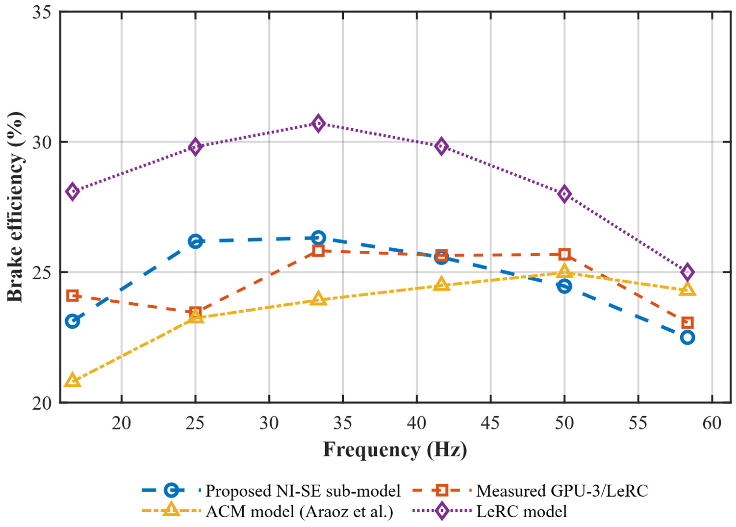
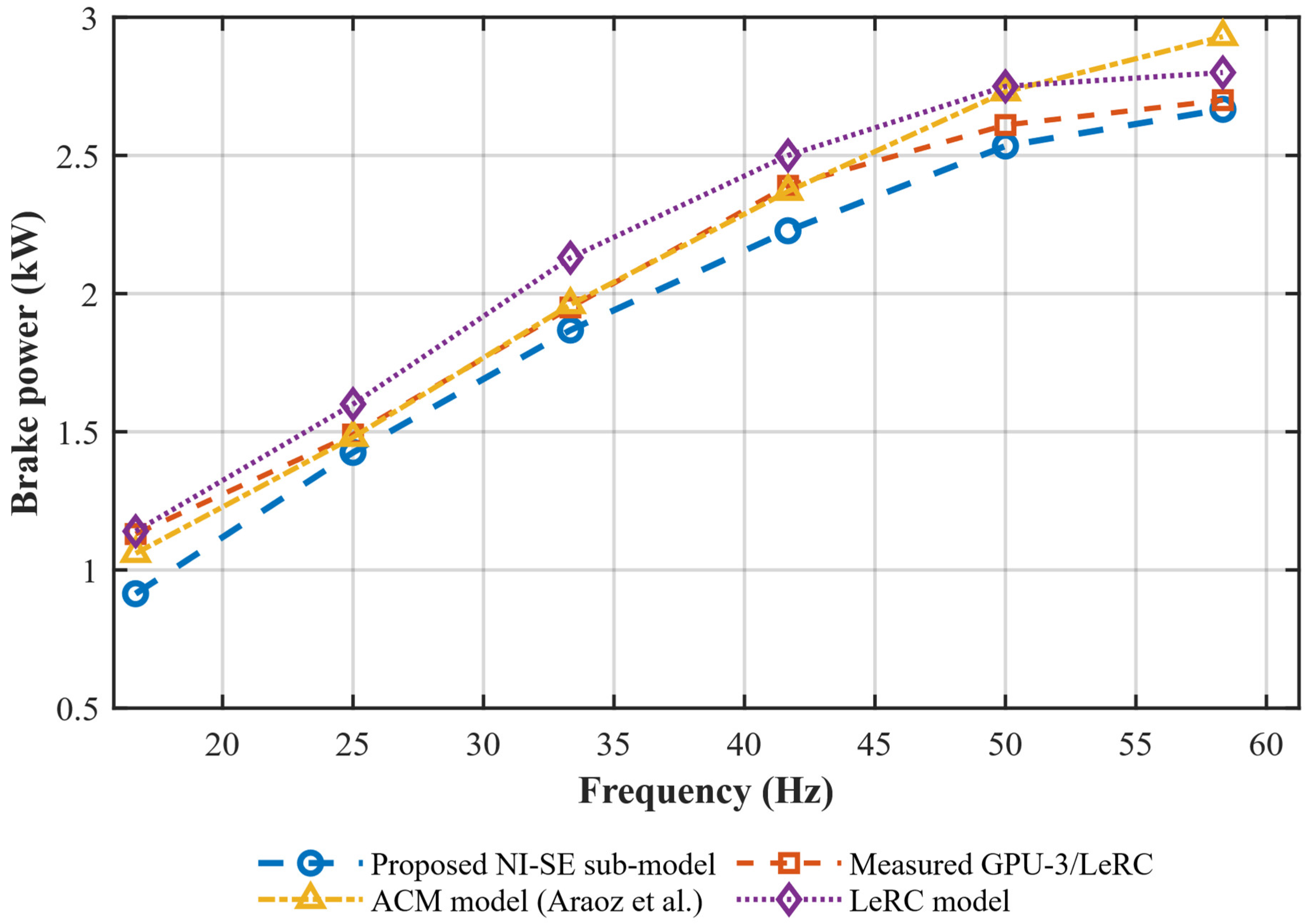
Next, the NI-SE model was validated against the GPU-3/LeRC benchmark used by Araoz et al. [21]. This validation isolates the internal Stirling engine thermodynamics, heat transfer, and loss submodels from the solar front-end and, therefore, tests whether the present implementation reproduces the known standalone engine behavior before receiver coupling is introduced. Figure 7 and Figure 8 compare the predicted brake efficiency and brake power, respectively, against the measured GPU-3 data [39,41], the LeRC model, and the ACM benchmark of Araoz et al. [21].

The comparison shows that the present NI-SE implementation reproduces the standalone frequency dependence of GPU-3 brake performance with an accuracy comparable to established benchmark models. In particular, the model captures the monotonic increase in brake power with frequency and the associated brake efficiency trend under the prescribed thermal boundary conditions. This agreement confirms that the present implementation of the non-ideal adiabatic Araoz framework remains a suitable standalone engine core before it is embedded in the receiver-coupled PSDS model.

To quantify the global agreement across the full tested frequency range, a statistical error analysis was performed against the LeRC experimental measurements, summarized in

Table 4. Global error metrics for standalone NI-SE validation against the GPU-3/LeRC benchmark, with comparison to the ACM model of Araoz et al. and the LeRC reference model [21].

Model	${\mathit{P}}_{\mathit{b}\mathit{r}}$ ME (kW)	${\mathit{P}}_{\mathit{b}\mathit{r}}$ NMAE (%)	${\mathit{P}}_{\mathit{b}\mathit{r}}$ RMSE (kW)	${\mathsf{\eta }}_{\mathit{b}\mathit{r}}$ ME (%-pts)	${\mathsf{\eta }}_{\mathit{b}\mathit{r}}$ NMAE (%)	${\mathsf{\eta }}_{\mathit{b}\mathit{r}}$ RMSE (%-pts)
Proposed NI-SE submodel	−0.106	5.17	0.123	0.07	4.1	1.32
ACM model (Araoz et al. [21])	0.043	3.75	0.110	−1.00	5.75	1.73
LeRC model	0.108	5.30	0.120	3.95	16.03	4.22

. The proposed NI-SE submodel yields brake power errors of the same order as the ACM and LeRC benchmark models, while maintaining improved brake efficiency agreement for the present dataset. In particular, the proposed formulation gives an NMAE of 5.17% and RMSE of 0.123 kW in brake power, together with an NMAE of 4.10% and RMSE of 1.32 percentage points in brake efficiency. These values support the use of the present NI-SE formulation in subsequent receiver-coupled PSDS simulations.

From a model development perspective, this standalone validation is especially valuable because it shows that the pressure-dependent heat transfer conductances, cycle-integrated pumping loss treatment, regenerator loss handling, and Qu-mode-ready numerical structure preserve the principal non-ideal thermodynamic penalties represented in the GPU-3 benchmark while still reproducing the classical Araoz-type engine behavior. Accordingly, the discrepancies observed later at the integrated system level can be interpreted primarily in terms of receiver engine coupling assumptions and system-level loss channels, rather than as deficiencies of the standalone engine core.

3.3. Integrated PSDS Validation Against EuroDish

Finally, the fully coupled PSDS model was validated against EuroDish system data. The EuroDish benchmark state reported by Reinalter et al. and Nepveu et al. [5,10] was used as the integrated operating reference, and the resulting receiver heat, cooler rejection, and electrical output were compared against the EuroDish dispatch and power partition data reported in the same studies. This stage tested the entire coupled chain: the EuroDish adapted dish/receiver/package front-end, the variable charge (Qu-mode) Stirling engine submodel, and the final electrical output calculation.

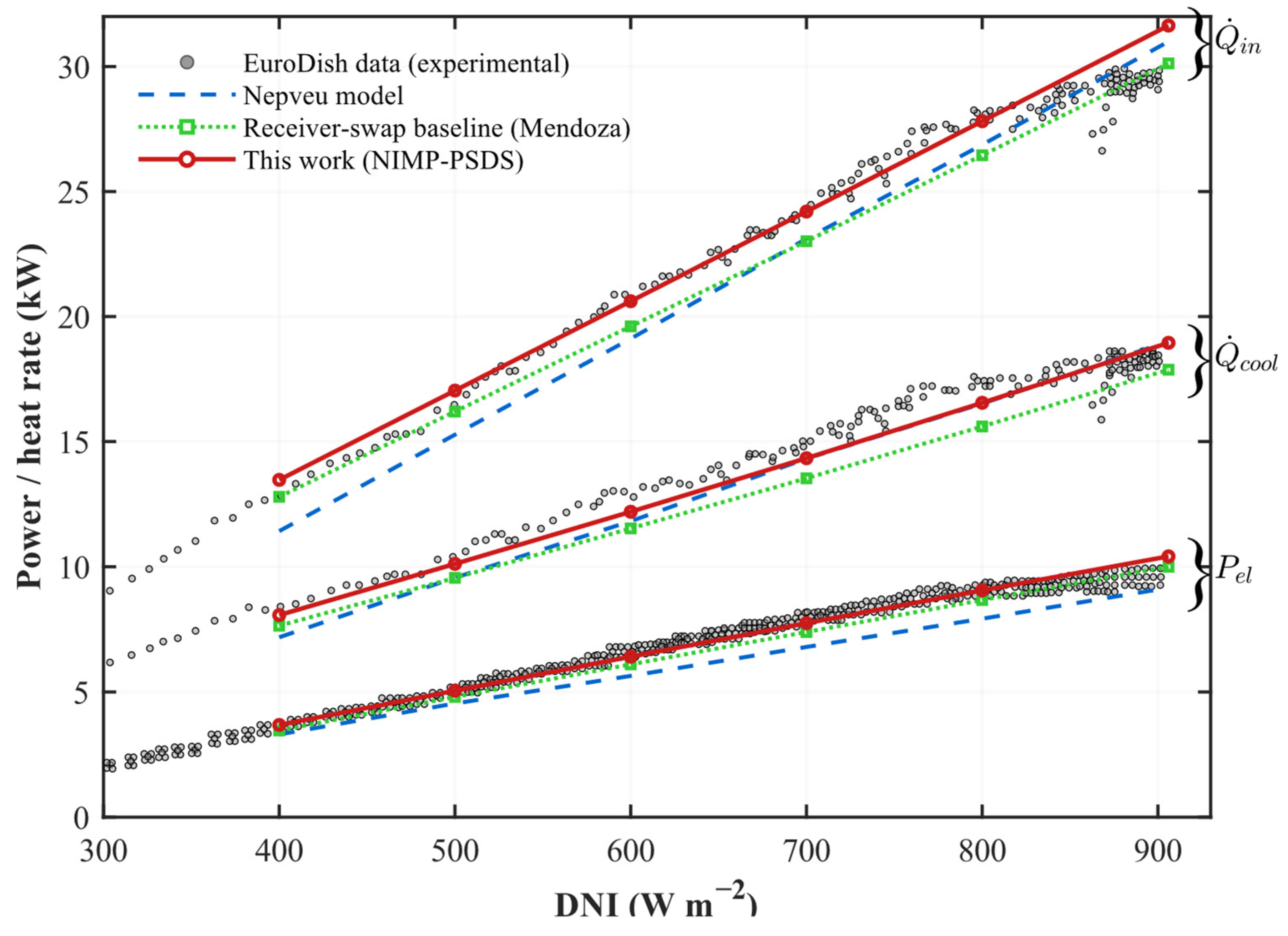
Figure 9 compares the predicted and reference powers delivered to the Stirling engine $\left({\dot{Q}}_{in}\right)$, rejected to the cooler (${\dot{Q}}_{cool})$, and exported electrically ${(P}_{\mathit{el-net}})$ as a function of DNI generated by the NIMP-PSDS model, the published Nepveu model [10], and a receiver swap baseline, in which a Mendoza-type receiver formulation is retained in place of the EuroDish-specific receiver front-end adopted in the present work. As can be gleaned from the figure, the proposed NIMP-PSDS model reproduces the main EuroDish power trends over the validation range while preserving the correct ordering and magnitude of the three energy channels. This comparison simultaneously exercises the receiver optics, cavity losses, package loss channel, engine heat uptake, cooling rejection, generator conversion, and parasitic consumption.

Table 5. Integrated EuroDish validation errors for net electrical power, heat input to the engine, and cooler rejection: comparison of the proposed NIMP-PSDS model, the Nepveu model [10], and the receiver swap baseline.

Model	${\mathit{P}}_{\mathit{el-net}}$ MAE/ RMSE (kW)	${\dot{\mathit{Q}}}_{\mathit{i}\mathit{n}}$ MAE/ RMSE (kW)	${\dot{\mathit{Q}}}_{\mathit{c}\mathit{o}\mathit{o}\mathit{l}}$ MAE/ RMSE (kW)	${\mathit{P}}_{\mathit{el-net}}$ MAPE/ RMSPE (%)	${\dot{\mathit{Q}}}_{\mathit{i}\mathit{n}}$ MAPE/ RMSPE (%)	${\dot{\mathit{Q}}}_{\mathit{c}\mathit{o}\mathit{o}\mathit{l}}$ MAPE/ RMSPE (%)
The proposed NIMP-PSDS model	0.300/0.385	0.624/0.907	0.569/0.606	4.28/5.03	2.90/3.81	4.07/4.14
Nepveu model [10]	0.754/0.873	1.331/1.338	0.887/0.911	10.26/11.33	6.62/6.99	7.29/8.14
Receiver swap baseline (Mendoza)	0.388/0.444	0.808/0.998	1.068/1.171	5.07/5.68	3.34/4.03	8.11/8.61

reports the MAE/RMSE and MAPE/RMSPE at the six common DNI points relative to the experimental reference curves extracted from Figure 9 of Nepveu et al. [10] for the proposed NIMP-PSDS model (4.28/5.03% for $P_{el,net}$, 2.9/3.81% for ${\dot{Q}}_{in}$, and 4.07/4.14% for ${\dot{Q}}_{cool}$), the Nepveu model, and the receiver swap baseline. Across the three validated output channels, the proposed model yields the lowest error levels among the compared alternatives for the present validation set, indicating that the receiver/package refinements and the coupled Qu-mode engine solution improve agreement relative to both the published Nepveu et al. [10] thermal model and the Mendoza et al. [17] receiver baseline embedded in the present framework. Thus, the NIMP-PSDS model is not only internally consistent but also predictive over the validated EuroDish operating range.

The receiver swap baseline in Table 5 also provides a combined receiver formulation comparison for the final aperture emission and wind convection treatment. In this baseline, the downstream Qu-mode engine coupling is retained, but the final EuroDish receiver formulation is replaced by the Mendoza-type receiver treatment. Thus, the comparison isolates the system-level effect of the final receiver formulation relative to the inherited receiver baseline, rather than re-tuning the downstream engine model. Relative to the receiver swap baseline, the final formulation reduces $P_{el,net}$ MAPE from 5.07% to 4.28%, ${\dot{Q}}_{in}$ MAPE from 3.34% to 2.90%, and ${\dot{Q}}_{cool}$ MAPE from 8.11% to 4.07%. The larger reduction in ${\dot{Q}}_{cool}$ MAPE supports the consistency of the propagated receiver engine thermal balance, since cooler rejection is a downstream heat flow output of the coupled model.

A further strength of this integrated validation is that it preserves loss channel traceability. Because the receiver, package, engine, cooler, generator, and parasitic terms are all carried explicitly, the model can be validated not only in terms of the final net electricity but also in terms of the intermediate heat flows that shape the EuroDish dispatch. The corresponding dispatch comparison is shown in Figure 10. This provides a stronger basis for the later transferability and parametric studies than would be obtained from a single-output validation alone.

3.4. Transferability Across Dish–Stirling Platforms

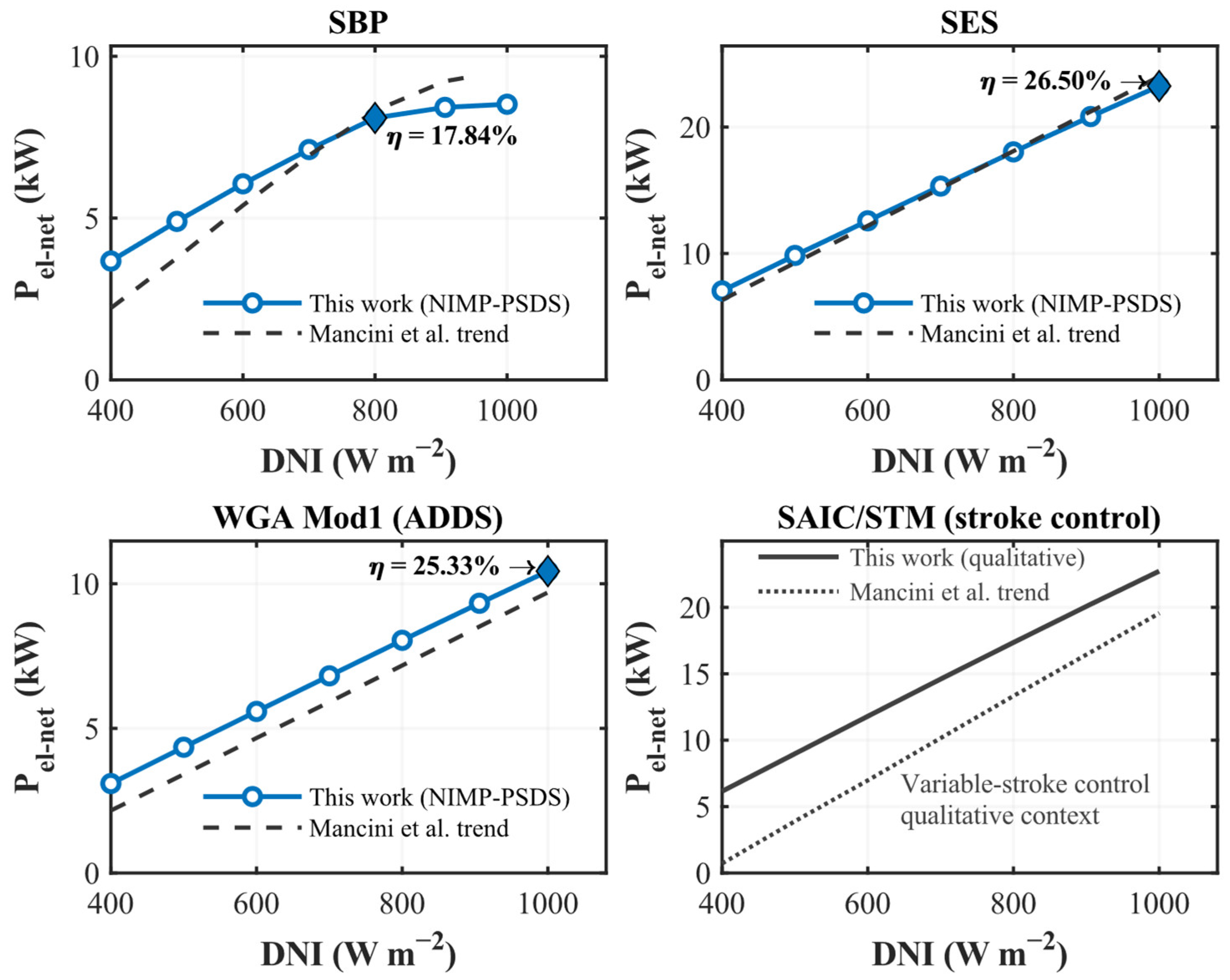
Using the transferability setup defined in Section 2.9, the proposed PSDS framework was re-parameterized for the representative systems SBP, SES, WGA Mod1 (ADDS), and SAIC/STM. A comparison of the resulting net electrical power trends against the Mancini reference curves [4] in Figure 11 reveals that for the three pressure-controlled systems (SBP, SES, and WGA Mod1) the model reproduces the overall $P_{el}\left(DNI\right)$ behavior with good agreement across the irradiance range. SES shows the closest overall match in both shape and magnitude, WGA-Mod1 is slightly overpredicted across most of the range while the correct slope is preserved. SBP is well captured at the design region but exhibits a somewhat flatter high-DNI response than the corresponding Mancini trend. The SAIC/STM case is shown for qualitative reference only.

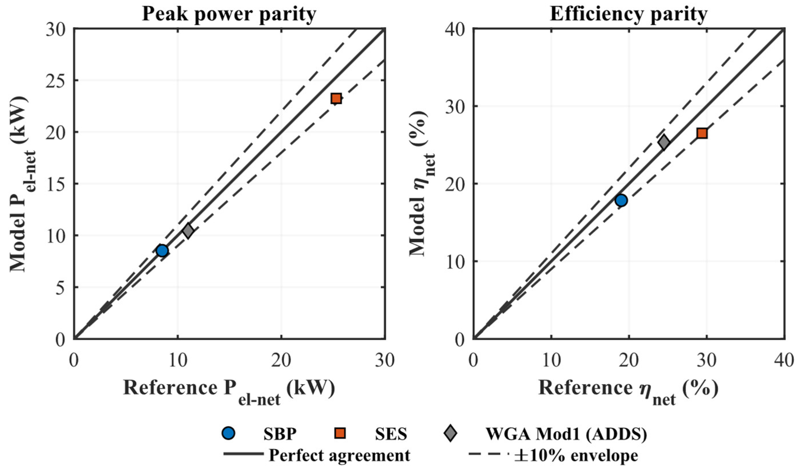
The peak point comparison, using parity plots, leads to the same conclusion (Figure 12). Specifically, parity was evaluated at the Mancini reference operating points; for net electrical power, at $DNI=1000 W{m}^{-2}$ for SBP, SES, and WGA Mod1 (ADDS), and for net efficiency, at $DNI=1000 W{m}^{-2}$ for SES and WGA Mod1 and at the reported SBP design point condition of $DNI=800 W{m}^{-2}$. Under those reference conditions, the predicted peak net electrical power remains within +0.22% for SBP, −8.13% for SES, and −5.14% for WGA Mod1 relative to the Mancini values [4]. The corresponding peak net efficiency deviations are −6.08% for SBP, −9.85% for SES, and +3.38% for WGA Mod1. Hence, all three quantitatively assessed systems remain within the $\pm 10\%$ parity envelope in terms of both peak power and peak efficiency, without introducing platform-specific recalibration.

For the three quantitatively assessed systems, the transferability errors are structured rather than random. The SES case is slightly underpredicted in both peak power and efficiency, suggesting that the standardized secondary assumptions used here are somewhat conservative for that platform. WGA Mod1 shows mild efficiency overprediction together with acceptable power agreement, which is consistent with the simplified multi-cylinder scaling and the use of a common receiver loss baseline. SBP shows nearly exact peak power agreement but a modest efficiency deficit, indicating that the unified cold-side, package loss, and parasitic assumptions likely affect efficiency more strongly than gross power scaling for that system.

Overall, within the limited public input reassignment used here, the pressure-controlled SBP, SES, and WGA Mod1 cases preserve the main $P_{el}\left(DNI\right)$ trends, order of magnitude, and peak performance levels within the $\pm 10\%$ parity envelope. The SAIC/STM curve is retained as qualitative context because its variable stroke architecture differs from the mean pressure/charge control formulation used in the present model. The structured deviations in SBP, SES, and WGA Mod1 point to the platform details that would be most valuable for future system-specific refinement, especially receiver loss coefficients, auxiliary loads, cooling conditions, and control implementation. In this sense, the transferability study supports the use of the framework for design-oriented comparison and sensitivity screening under limited public system data, while identifying the additional information needed for platform-specific prediction.

3.5. Parametric Sensitivity/Capability Studies

Next, the coupled PSDS model was evaluated for its representative parametric sensitivities and capability trade-offs, focusing on engine speed, heat exchanger scaling, environmental conditions, and cooling boundary limitations, illustrating the design-oriented utility of the coupled PSDS model.

3.5.1. Engine Speed Sweep

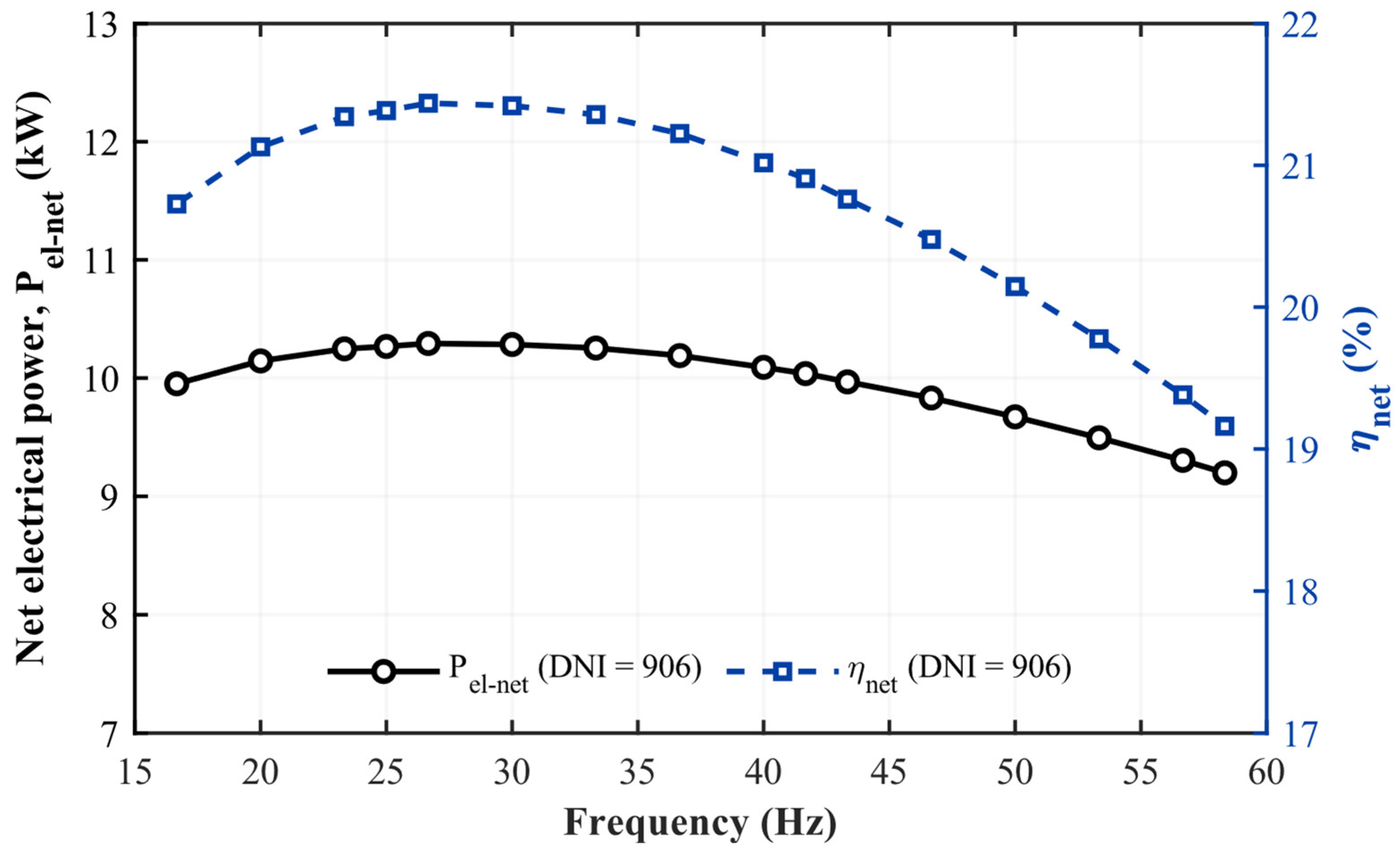
At fixed validated EuroDish receiver/package heat input, ${\dot{Q}}_{u\to h}=31.63 kW$, and fixed $R_{ref}$, the Qu-mode speed sweep reveals a broad optimum in the nominal operating range. As shown in Figure 13, $P_{el}$ increases from 9.95 kW at 1000 rpm to a broad optimum of about 10.29 kW over the range 1500–2000 rpm, before decreasing to 9.2 kW at 3500 rpm. The net efficiency follows the same pattern. Over the same range, the cycle mean pressure decreases monotonically from 21.67 MPa to 6.47 MPa, consistent with the charge reduction required by variable charge control (Qu-mode) to satisfy the fixed heat match constraint.

Because the receiver-side input is held fixed in this sweep, the resulting trends isolate engine internal behavior. As summarized in

Table 6. Loss channel and power decomposition for the engine speed sweep at fixed validated EuroDish receiver/package input ${\dot{\mathit{Q}}}_{\mathit{u}\mathbf{\to }\mathit{h}}\mathbf{=}\mathbf{31.63} \mathit{k}\mathit{W}$ and fixed ${\mathit{R}}_{\mathit{r}\mathit{e}\mathit{f}}$.

Engine Speed (RPM)	Mean Pressure (MPa)	Internal Conduction Losses ${\dot{\mathit{Q}}}_{\mathit{l}\mathit{k}}$ (kW)	Shuttle Conduction Losses ${\dot{\mathit{Q}}}_{\mathit{l}\mathit{s}\mathit{h}}$ (kW)	Regenerator Losses ${\dot{\mathit{Q}}}_{\mathit{l}\mathit{o}\mathit{s}\mathit{s}\mathit{r}}$ (kW)	${\dot{\mathit{Q}}}_{\mathit{c}\mathit{o}\mathit{o}\mathit{l}}$ (kW)	Friction Losses ${\mathit{W}}_{\mathit{f}\mathit{r}\mathit{i}\mathit{c}}$ (kW)	Indicated Power (kW)	Electrical Output ${\mathit{P}}_{\mathit{e}\mathit{l}}$ (kW)
1000	21.67	0.45	1.31	2.79	20.09	1.18	12.46	9.95
1500	14.73	0.45	1.34	2.88	19.02	1.51	13.13	10.27
1600	13.86	0.45	1.34	2.89	18.9	1.58	13.23	10.29
1800	12.36	0.46	1.35	2.91	18.62	1.74	13.38	10.28
2000	11.17	0.46	1.35	2.93	18.42	1.91	13.52	10.25
2500	8.99	0.46	1.36	2.96	18.02	2.39	13.76	10.04
3000	7.52	0.46	1.36	2.98	17.73	2.95	13.93	9.67
3500	6.47	0.46	1.37	2.99	17.53	3.60	14.06	9.20

, the regenerator shortfall loss ${\dot{Q}}_{lossr}$ increases only modestly $\left(2.79\to 2.99 \mathrm{kW}\right),$ because increasing $N$ raises the oscillatory mass flow frequency and characteristic velocity through the regenerator, thereby reducing the effective regenerator NTU and effectiveness in the model. The internal conduction leak ${\dot{Q}}_{lk}$ remains nearly constant $\left(\approx 0.45-0.46 kW\right),$ consistent with a geometry and $\Delta T$-dominated conduction path rather than a speed-dependent mechanism, while the shuttle term ${\dot{Q}}_{lsh}$ changes only weakly $(1.31 \to 1.37 kW)$, consistent with its weak dependence on the cycle temperature swing. By contrast, the total friction/pumping loss $W_{fric}=W_{ploss}+W_{mech}$ rises strongly, from 1.18 kW to 3.60 kW, whereas the indicated power increases only moderately, from 12.46 kW to 14.06 kW. The speed optimum, therefore, reflects a balance between improved power conversion at moderate frequency and increasingly adverse internal dissipation at high rpm.

3.5.2. Heat Exchanger Scaling Sweep

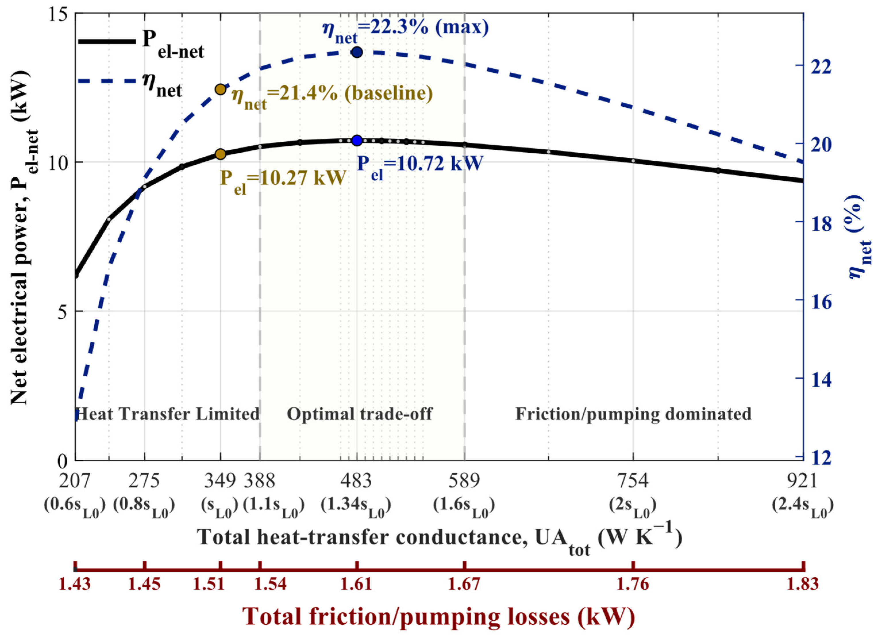
Figure 14 summarizes the heat exchanger scaling sweep in terms of net electrical output, net efficiency, overall conductance, and total friction losses, where $U{A}_{tot}={\displaystyle \raisebox{1ex}{$1$}\!\left/ \!\raisebox{-1ex}{$2$}\right.}\left(U{A}_h+U{A}_k\right)$ and $W_{fric}=W_{ploss}+W_{mech}$.

Increasing the common length scale $s_L$ initially increases $U{A}_{tot}$ and raises $P_{\mathit{el-net}}$, indicating a heat-transfer-limited regime at low exchanger size. Relative to the baseline case $\left(P_{\mathit{el-net}}\approx 10.27 \mathrm{kW}, {\eta }_{net}\approx 21.4\%\right)$, the sweep reaches a broad near-optimal region, with a maximum of about $P_{el,max}\approx 10.72 \mathrm{kW}$ and ${\eta }_{net}\approx 22.3\%$. Using the ${ϵ}_{MGA}=2\%$ criterion (Section 2.10), the near-optimal band (trade-off band) spans approximately $U{A}_{tot}=388÷589 W{K}^{\mathrm{-1}}.$ Beyond this near-optimal region, further increases in exchanger size do not improve the net output. Instead, $P_{\mathit{el-net}}$ begins to decline while total friction losses continue to rise (friction/pumping-dominated regime).

This behavior is consistent with the underlying sweep physics: increasing $l_h$ and $l_c$ raises the heat transfer area and thus improves $U{A}_h$ and $U{A}_k$, but it also increases the heater/cooler dead volumes (Appendix A) and the flow length, which respectively reduce the effective pressure swing and increase the hydraulic dissipation. The resulting optimum, therefore, reflects a balance between improved heat transfer capability at moderate $s_L$ and higher friction/pumping penalties at larger exchanger sizes. In this sense, the sweep identifies a practically useful near-optimal design region rather than a single isolated optimum.

3.5.3. Environmental Sweep $\left(T_a,wind\right)$

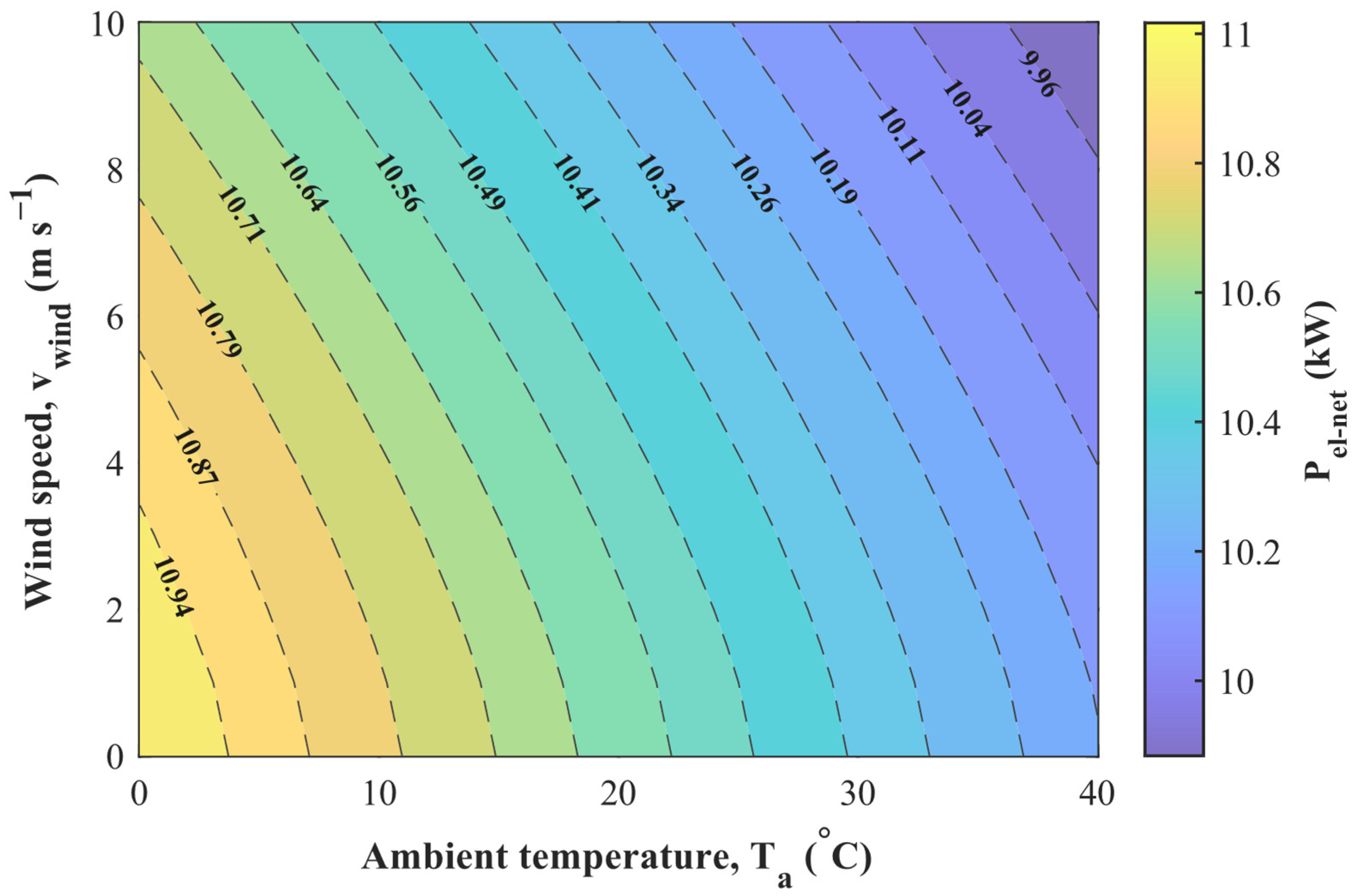
At a fixed DNI = 906 $W{m}^{-2}$ and baseline heat exchanger geometry, Figure 15 shows the predicted net electrical power over the environmental domain $T_a$ = 273.15 to 313.15 K and $v_{wind}$ = 0 to 10 $m{s}^{-1}$. For each operating point, the effective receiver cooling factor $R_{ref,eff}\left(T_a,v_{wind}\right)$ was re-identified through the receiver engine energy balance procedure, after which the final system state is solved in variable charge control (Qu-mode). The resulting power field varies smoothly and monotonically across the domain, from a maximum of 11.017 kW at $T_a$ = 273.15 K and $v_{wind}$ = 0 $m{s}^{-1}$, to a minimum of 9.884 kW at $T_a$ = 313.15 K and $v_{wind}$ = 10 $m{s}^{-1}$. The nominal baseline point ($T_a$ = 288 K, $v_{wind}$ = 1.5 $m{s}^{-1}$) gives 10.687 kW. The nearly parallel diagonal contours indicate that no interior optimum exists within the investigated range; instead, power decreases progressively with both increasing ambient temperature and increasing wind speed.

The sensitivity is stronger with respect to ambient temperature than to wind over the investigated EuroDish operating range. At the baseline ambient temperature of 288 K, increasing wind speed from 0 to 10 $m{s}^{-1}$ reduces $P_{\mathit{el-net}}$ by 0.322 kW (3.0%). By contrast, at the baseline wind speed of 1.5 $m{s}^{-1}$, increasing ambient temperature from 273.15 K to 313.15 K reduces $P_{el}$ by 0.816 kW (7.4%). The wind speed effect enters mainly through the receiver-side forced convection/aperture loss path; stronger wind increases receiver external cooling and lowers the useful heat delivered to the engine. Ambient temperature affects a broader set of coupled pathways. It changes receiver/package heat exchange and, under the fixed-approach cooling boundary closure used in the sweep, also raises the imposed Stirling cold-side boundary. Although warmer ambient conditions can partially reduce some receiver-to-ambient and package-to-ambient temperature differences, the hotter cold-side boundary reduces the effective Stirling temperature span and net conversion efficiency. Consequently, ambient temperature produces the larger net electrical-output penalty in this sweep, while wind remains a relevant receiver loss mechanism within the tested range. The net result is a smooth contraction of electrical output under worsening environmental conditions. The robustness of the identified near-optimal $s_L$ region under ambient variability was examined separately using capability envelopes of $P_{\mathit{el-net}}$ over the $(T_a,v_{wind})$ domain; the full envelope plot is provided in Supplementary Figure S1.

3.5.4. Cold Boundary Sweep $\left(T_{wok,BC}/\Delta T_{app}\right)$

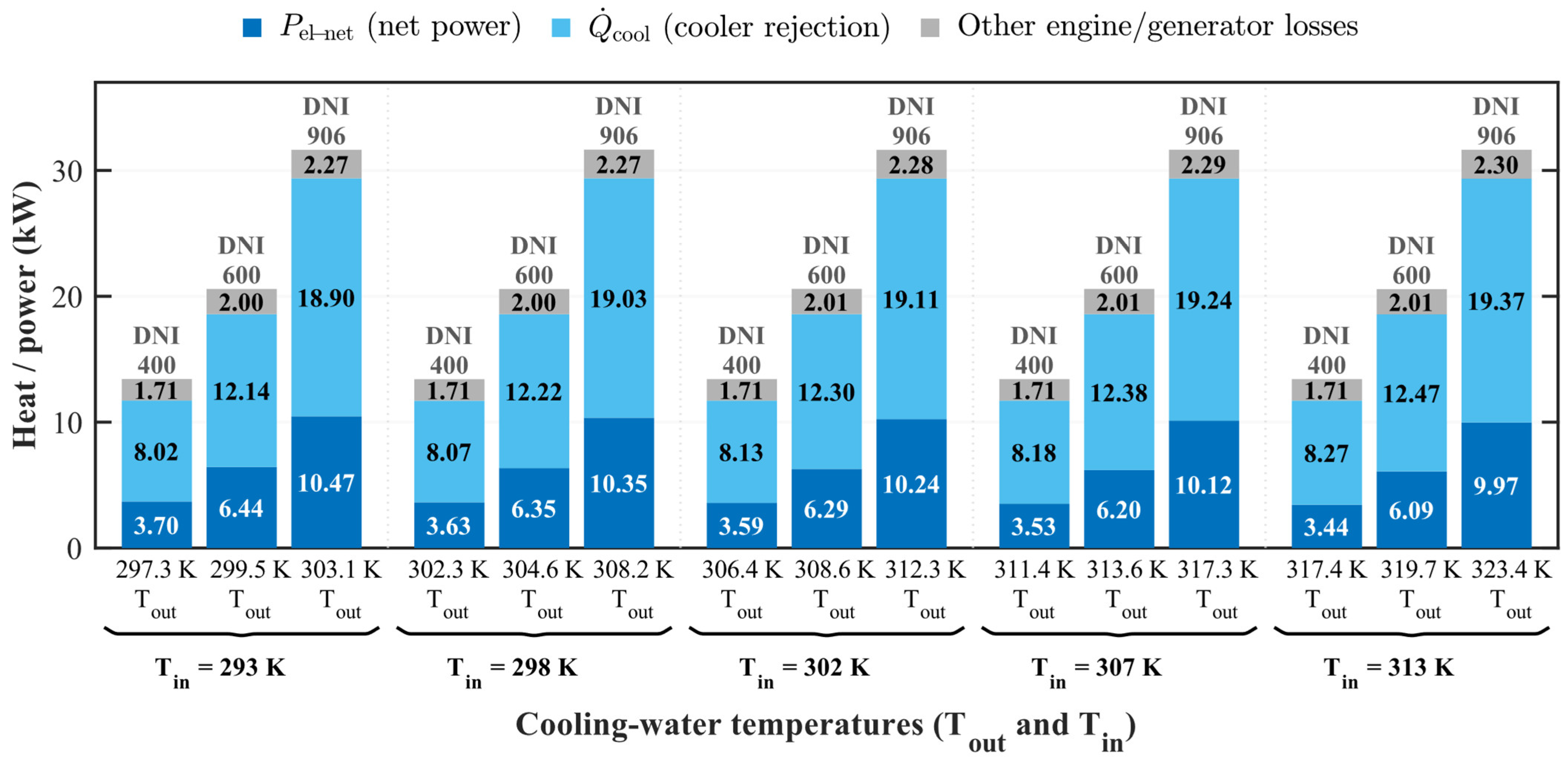
Figure 16 shows the effect of increasing the imposed cooling water (coolant) inlet temperature on the system energy distribution at DNI = 400, 600, and 906 $W{m}^{-2}$. For each irradiance level, the receiver/package front-end input was held fixed, so the sweep isolates the response of the coupled Stirling engine subsystem to a degraded cold-side boundary.

As the imposed inlet temperature rises from 293 to 313 K for a coolant volume flow rate of ${\dot{V}}_{cool}=4.92·{10}^{-4} m^3{s}^{-1}$, net electrical power decreases monotonically for all three DNI levels, while cooler rejection increases correspondingly. Because the coolant flow rate and coolant specific heat ($c_{p,cool})$ are fixed in this sweep, Equation (56) links the outlet water temperature to the imposed inlet temperature and the heat rejected to the cooling stream. The outlet water temperature therefore rises with the imposed inlet temperature, while the higher-DNI cases remain at higher outlet temperature levels because their larger receiver/package thermal input produces a larger cooler rejection duty.

The magnitude of the electrical power penalty increases in absolute terms with DNI. At $DNI=400 W{m}^{-2}$, $P_{\mathit{el-net}}$ decreases from 3.70 kW to 3.44 kW as $T_{coolant,in}\equiv T_{wok,BC }$ rises from 293 to 313 K, whereas at $DNI=600 W{m}^{-2}$ it decreases from 6.44 kW to 6.09 kW, and at $DNI=906 W{m}^{-2}$ from 10.47 kW to 9.97 kW. Over the same interval, ${\dot{Q}}_{cool}$ increases from 8.02 kW to 8.27 kW at $DNI=400 W{m}^{-2}$, from 12.14 kW to 12.47 kW at $DNI=600 W{m}^{-2}$, and from 18.90 kW to 19.37 kW at $DNI=906 W{m}^{-2}$. By contrast, the remaining loss block changes only weakly. Because the supplied thermal input remains essentially unchanged for each DNI case, the main effect of a warmer cooling sink is therefore to redistribute the fixed receiver/package heat input away from electrical output and into rejected heat. This behavior is consistent with the engine-side physics of the sweep. A hotter imposed cold-side boundary reduces the effective temperature span of the Stirling cycle and therefore lowers the net conversion efficiency, while the fixed front-end heat input is redirected primarily into cooler rejection rather than into large changes in the remaining losses. The result is important from a system design perspective: degraded cooling conditions do not only reduce electrical performance but also increase the co-produced rejected heat available for downstream thermal utilization.

4. Conclusions

This study presented a modular, energy-consistent NIMP-PSDS framework that couples a EuroDish-adapted dish/receiver/package front-end to a non-ideal Stirling engine model through variable charge heat matching. By combining receiver package engine coupling, explicit loss channel traceability, and control-consistent receiver engine heat matching in a compact system-level formulation, the framework provides a practical, loss-resolved basis for PSDS design studies, loss diagnosis, and control-oriented analysis. The main contributions are (i) a receiver/package/non-ideal Stirling coupling strategy under variable charge operation; (ii) an explicit loss traceability framework resolving optical, receiver, package, engine, generator, parasitic, and cooler rejection channels; and (iii) a Qu-mode receiver engine thermal matching solution in which the operating point emerges from a closed energy balance rather than from prescribed hot-side temperature, fixed heat input, or prescribed mean pressure.

The staged verification and validation strategy showed that the inherited Mendoza receiver backbone was implemented consistently, so that the standalone engine core reproduced GPU-3/LeRC behavior with benchmark-level agreement, and that the fully coupled model reproduced EuroDish dispatch while yielding the lowest integrated error levels among the compared alternatives for the present validation set. At the integrated EuroDish level, the model reproduced heat input, cooler rejection, and net electrical output with MAPE values of 2.90%, 4.07%, and 4.28%, respectively. Relative to the detailed spatial modeling of Nepveu et al. [10], the present framework retains key loss mechanisms while achieving the computational speed required for extensive parametric sweeps. Relative to the performance analysis of Reinalter et al. [5], this work provides a predictive integrated model that reproduces EuroDish dispatch while explicitly tracking and propagating loss channels through the coupled simulation.

Taken together, these results demonstrate that the framework is sufficiently detailed to retain channel-by-channel physical traceability, yet compact enough for transferability and capability studies. The limited-input transferability assessment further supports the framework’s use for design-oriented comparison and sensitivity screening: for the quantitatively assessed pressure-controlled systems, the model preserved order of magnitude, trend behavior, and peak performance levels within the $\pm 10\%$ envelope under public-input reassignment. SAIC/STM was retained as qualitative context because its variable-stroke control differs from the mean pressure/charge control formulation represented here. The structured deviations highlight the platform-specific information most valuable for future refinement, particularly receiver loss coefficients, auxiliary/parasitic loads, cooling-system conditions, and control implementation.

The parametric studies further showed physically interpretable trends: engine speed exhibits a broad optimum, exchanger sizing leads to a broad near-optimal region rather than a single sharp optimum, ambient temperature has a stronger effect on net output than wind over the tested range, and degraded cooling conditions primarily redirect fixed thermal input from electricity to rejected heat.

The results also indicate the main limitations of the present framework and the corresponding paths for refinement. The current formulation is quasi-steady and, by design, uses EuroDish reference point receiver/package anchoring, compact engineering receiver/package heat loss closures, and public rather than platform-resolved BOP/control information for transferability cases. Additional raw off-design and time-resolved validation data, together with platform-specific receiver loss, cooling system, auxiliary load, and control characterization inputs, would improve system-specific prediction and extend confidence beyond the present benchmarked operating space. Because cooler rejection is resolved explicitly, a natural extension is to examine the utilization of the rejected heat stream in secondary thermal applications, including desalination, cooling load production, storage-assisted operation, or other hybrid solar–thermal uses. Finally, extending the formulation to architectures not explicitly represented here, including variable stroke systems, and embedding it in uncertainty-aware parameter identification, optimization, or control studies would further strengthen its value as a predictive design and analysis tool for dish–Stirling and related hybrid solar–thermal systems.

References

1. Abdelhay, A.; Fath, H.S.; Nada, S.A. Solar driven polygeneration system for power, desalination and cooling. Energy 2020, 198, 117341. [Google Scholar] [CrossRef] [Scilit]
2. Siva Reddy, V.; Kaushik, S.C.; Tyagi, S.K. Exergetic analysis and performance evaluation of parabolic dish Stirling engine solar power plant. Int. J. Energy Res. 2013, 37, 1287–1301. [Google Scholar] [CrossRef] [Scilit]
3. Mehrpooya, M.; Ghadimi, N.; Marefati, M.; Ghorbanian, S.A. Numerical investigation of a new combined energy system includes parabolic dish solar collector, Stirling engine and thermoelectric device. Int. J. Energy Res. 2021, 45, 16436–16455. [Google Scholar] [CrossRef] [Scilit]
4. Mancini, T.; Heller, P.; Butler, B.; Osborn, B.; Schiel, W.; Goldberg, V.; Buck, R.; Diver, R.; Andraka, C.; Moreno, J. Dish-stirling systems: An overview of development and status. J. Sol. Energy Eng. 2003, 125, 135–151. [Google Scholar] [CrossRef] [Scilit]
5. Reinalter, W.; Ulmer, S.; Heller, P.; Rauch, T.; Gineste, J.-M.; Ferrière, A.; Nepveu, F. Detailed performance analysis of a 10 kW dish/Stirling system. J. Sol. Energy Eng. 2008, 130, 011013. [Google Scholar] [CrossRef] [Scilit]
6. Malik, M.Z.; Shaikh, P.H.; Zhang, S.; Lashari, A.A.; Leghari, Z.H.; Baloch, M.H.; Memon, Z.A.; Caiming, C. A review on design parameters and specifications of parabolic solar dish Stirling systems and their applications. Energy Rep. 2022, 8, 4128–4154. [Google Scholar] [CrossRef] [Scilit]
7. Kumar, R.; Thakur, A.K.; Gupta, L.R.; Gehlot, A.; Sikarwar, V. Advances in phase change materials and nanomaterials for applications in thermal energy storage. Environ. Sci. Pollut. Res. 2023, 31, 6649–6677. [Google Scholar] [CrossRef] [Scilit]
8. Malik, A.Q.; Jabeen, T.; Jabeen, I.; Mubarak, N.M.; Hosseini-Bandegharaei, A.; Najeeb, A.; Nawaz, R.; Abnisa, F. Holistic insight mechanism of nano-based phase change for thermal storage applications. Results Surf. Interfaces 2025, 20, 100579. [Google Scholar] [CrossRef] [Scilit]
9. Aboelmaaref, M.M.; Zhao, J.; Li, W.; Ali, E.S.; Askalany, A.A.; Ghazy, M.; Gu, L.; Zayed, M.E. Research on solar dish/Stirling engine driven adsorption-based desalination system for simultaneous co-generation of electricity and freshwater: Numerical investigation. Case Stud. Therm. Eng. 2023, 47, 103044. [Google Scholar] [CrossRef] [Scilit]
10. Nepveu, F.; Ferriere, A.; Bataille, F. Thermal model of a dish/Stirling systems. Sol. Energy 2009, 83, 81–89. [Google Scholar] [CrossRef] [Scilit]
11. Li, Y.; Choi, S.S.; Yang, C. Dish-Stirling Solar Power Plants: Modeling, Analysis, and Control of Receiver Temperature. IEEE Trans. Sustain. Energy 2014, 5, 398–407. [Google Scholar] [CrossRef] [Scilit]
12. Li, Y.; Choi, S.S.; Yang, C.; Wei, F. Design of Variable-Speed Dish-Stirling Solar–Thermal Power Plant for Maximum Energy Harness. IEEE Trans. Energy Convers. 2015, 30, 394–403. [Google Scholar] [CrossRef] [Scilit]
13. Howard, D.; Harley, R.G. Modeling of dish-Stirling solar thermal power generation. In Proceedings of the IEEE PES General Meeting, Minneapolis, MN, USA, 25–29 July 2010; pp. 1–7. [Google Scholar] [CrossRef] [Scilit]
14. Zayed, M.; Zhao, J.; Li, W.; Elsheikh, A.; Sadek, S.; Moustafa, M.A. A comprehensive review on Dish/Stirling concentrated solar power systems: Design, optical and geometrical analyses, thermal performance assessment, and applications. J. Clean. Prod. 2020, 283, 124664. [Google Scholar] [CrossRef] [Scilit]
15. AHafez, Z.; Soliman, A.; El-Metwally, K.A.; Ismail, I.M. Design analysis factors and specifications of solar dish technologies for different systems and applications. Renew. Sustain. Energy Rev. 2017, 67, 1019–1036. [Google Scholar] [CrossRef] [Scilit]
16. Livingston, F.R. Activity and Accomplishments in Dish/Stirling Electric Power System Development; Jet Propulsion Lab.: Pasadena, CA, USA, 1985. [Google Scholar] [CrossRef] [Scilit]
17. Castellanos, L.S.M.; Caballero, G.E.C.; Cobas, V.R.M.; Lora, E.E.S.; Reyes, A.M.M. Mathematical modeling of the geometrical sizing and thermal performance of a Dish/Stirling system for power generation. Renew. Energy 2017, 107, 23–35. [Google Scholar] [CrossRef] [Scilit]
18. Gil, R.; Monné, C.; Bernal, N.; Muñoz, M.; Moreno, F. Thermal Model of a Dish Stirling Cavity-Receiver. Energies 2015, 8, 1042–1057. [Google Scholar] [CrossRef] [Scilit]
19. Urieli, I.; Berchowitz, D.M. Stirling Cycle Engine Analysis; Adam Hilger: Bristol, UK, 1984. [Google Scholar]
20. Dyson, R.; Wilson, S.; Tew, R. Review of Computational Stirling Analysis Methods. In Proceedings of the 2nd International Energy Conversion Engineering Conference, Providence, RI, USA, 16–19 August 2004. NASA/TM-2004-213300. [Google Scholar]
21. Araoz, J.A.; Salomon, M.; Alejo, L.; Fransson, T.H. Non-ideal Stirling engine thermodynamic model suitable for the integration into overall energy systems. Appl. Therm. Eng. 2014, 73, 205–221. [Google Scholar] [CrossRef] [Scilit]
22. Howard, D.F.; Liang, J.; Harley, R.G. Control of receiver temperature and shaft speed in dish-Stirling solar power plants to meet grid integration requirements. In Proceedings of the 2010 IEEE Energy Conversion Congress and Exposition, Atlanta, GA, USA, 12–16 September 2010; pp. 398–405. [Google Scholar] [CrossRef] [Scilit]
23. Nazemi, S.D.; Boroushaki, M. Design, Analysis and Optimization of a Solar Dish/Stirling System. Int. J. Renew. Energy Dev. 2016, 5, 33–42. [Google Scholar] [CrossRef] [Scilit]
24. Buscemi, A.; Brano, V.L.; Chiaruzzi, C.; Ciulla, G.; Kalogeri, C. A validated energy model of a solar dish-Stirling system considering the cleanliness of mirrors. Appl. Energy 2020, 260, 114378. [Google Scholar] [CrossRef] [Scilit]
25. Sandoval, O.R.; Caetano, B.C.; Borges, M.U.; García, J.J.; Valle, R.M. Modelling, simulation and thermal analysis of a solar dish/Stirling system: A case study in Natal, Brazil. Energy Convers. Manag. 2019, 181, 189–201. [Google Scholar] [CrossRef] [Scilit]
26. Cheng, C.-H.; Huang, S.-T. Modeling of a hybrid power system integrating solar radiation and syngas combustion energy. Energy Sci. Eng. 2023, 11, 3379–3396. [Google Scholar] [CrossRef] [Scilit]
27. ProEcoPolyNet. Fact Sheet: SOLO Stirling 161. In Promotion of Eco-Building Technologies, Small Polygeneration and Renewable Heating & Cooling Technologies for Buildings; European Commission Sixth Framework Programme: Sindelfingen, Germany, 2007; Available online: https://build-up.ec.europa.eu/sites/default/files/content/SOLO%20Stirling%20161.pdf (accessed on 22 March 2026).
28. Stine, W.; Harrigan, B. Solar Energy Fundamentals and Design: With Computer Applications (Alternate Energy Series); Wiley-Interscience: Medford, MA, USA, 1985. [Google Scholar]
29. Samanes, J.; García-Barberena, J.; Zaversky, F. Modeling Solar Cavity Receivers: A Review and Comparison of Natural Convection Heat Loss Correlations. Energy Procedia 2015, 69, 543–552. [Google Scholar] [CrossRef] [Scilit]
30. Siebers, D.L.; Kraabel, J.S. Estimating Convective Energy Losses from Solar Central Receivers; Sandia National Laboratories Report: Albuquerque, NM, USA, 1984. [Google Scholar]
31. Clausing, A.M. An analysis of convective losses from cavity solar central receivers. Sol. Energy 1981, 27, 295–300. [Google Scholar] [CrossRef] [Scilit]
32. Ma, R.Y. Wind Effects on Convective Heat Loss from a Cavity Receiver for a Parabolic Concentrating Solar Collector; Sandia National Labs.: Albuquerque, NM, USA, 1993. [Google Scholar]
33. Schmidt, G. The theory of Lehmann’s calorimetric machine. Z. Ver. Dtsch. Ing. 1871, 15, 1–12. [Google Scholar]
34. Araoz, J.A.; Cardozo, E.; Salomon, M.; Alejo, L.; Fransson, T.H. Development and validation of a thermodynamic model for the performance analysis of a gamma Stirling engine prototype. Appl. Therm. Eng. 2015, 83, 16–30. [Google Scholar] [CrossRef] [Scilit]
35. Thombare, D.G.; Verma, S.K. Technological development in the Stirling cycle engines. Renew. Sustain. Energy Rev. 2008, 12, 1–38. [Google Scholar] [CrossRef] [Scilit]
36. Incropera, F.P.; Lavine, A.S.; DeWitt, D.P. Fundamentals of Heat and Mass Transfer, 6th ed.; John Wiley & Sons: Hoboken, NJ, USA.
37. Strauss, J.M.; Dobson, R.T. Evaluation of a second order simulation for Sterling engine design and optimization. J. Energy S. Afr. 2010, 21, 17–29. [Google Scholar] [CrossRef] [Scilit]
38. Timoumi, Y.; Tlili, I.; Nasrallah, S.B. Design and performance optimization of GPU-3 Stirling engines. Energy 2008, 33, 1100–1114. [Google Scholar] [CrossRef] [Scilit]
39. Tew, R.C., Jr.; Thieme, L.G.; Miao, D. Initial Comparison of Single Cylinder Stirling Engine Computer Model Predictions with Test Results. (DOE/NASA/1040-78/30), for sale by the National Technical Information Service. In Proceedings of the Congress and Exposition, Detroit, MI, USA, 10 October 1979. [Google Scholar]
40. Liu, C.-W.; Chuah, Y.-K. A study on an optimal approach temperature control strategy of condensing water temperature for energy saving. Int. J. Refrig. 2011, 34, 816–823. [Google Scholar] [CrossRef] [Scilit]
41. Thieme, L.G. Low-Power Baseline Test Results for the GPU 3 Stirling Engine; Report No. NASA TM-79103; NASA Lewis Research Center: Cleveland, OH, USA, 1979. [Google Scholar]
42. Tew, R.C.; Jefferies, K.; Miao, D. A Stirling Engine Computer Model for Performance Calculations; Department of Energy, Office of Conservation and Solar Applications, Division of Transportation Energy Conservation: Washington, DC, USA, 1978.
43. Price, J.; Keppo, I. Modelling to generate alternatives: A technique to explore uncertainty in energy-environment-economy models. Appl. Energy 2017, 195, 356–369. [Google Scholar] [CrossRef] [Scilit]
44. Martini, W.R. Stirling Engine Design Manual; University Press of the Pacific: Honolulu, HI, USA, 2004. [Google Scholar]
Figure 1. Physical and computational overview of the modeled PSDS framework. (a) EuroDish/SOLO-161 physical reference schematic informed by the CNRS EuroDish system configuration reported by Reinalter et al. [5] and by the geometry inputs summarized in Appendix C [5,10,27]. The panel identifies the parabolic reflective concentrator, support/tracking structure, receiver engine package, SOLO-161 package envelope, and reference concentrator geometry; package envelope dimensions are included for physical scale/proportion. (b) Integrated PSDS block diagram showing the coupled dish/receiver/package/Stirling engine/generator framework.
Applsci 16 05560 g001
Figure 2. Package loss network between receiver and ambient.
Applsci 16 05560 g002
Figure 3. Five-control-volume representation of the non-ideal adiabatic Stirling engine model used in the present work, based on the classical Urieli–Berchowitz [19] control volume decomposition and coupled here with non-ideal heat transfer and loss terms following Araoz et al. [21].
Applsci 16 05560 g003
Figure 4. Numerical solution sequence for the coupled Qu-mode PSDS.
Applsci 16 05560 g004
Figure 5. Verification of the implemented Mendoza receiver backbone against the closed-form receiver temperature relations reported in Mendoza et al. [17].
Applsci 16 05560 g005
Figure 6. Consistency check of the implemented Mendoza receiver backbone against the S1–S5 receiver cases reported in Mendoza Table 7 [17].
Applsci 16 05560 g006
Figure 7. Brake efficiency validation of the standalone NI-SE model against GPU-3/LeRC experimental data [39,41], the LeRC model [39,42], and the ACM model of Araoz et al. [21].
Applsci 16 05560 g007
Figure 8. Brake power validation of the standalone NI-SE model against GPU-3/LeRC experimental data [39,41], the LeRC model [39,42], and the ACM model of Araoz et al. [21].
Applsci 16 05560 g008
Figure 9. Integrated EuroDish validation: comparison of heat input to the Stirling engine, cooler rejection, and net electrical output versus DNI in the experiment [5,10], Nepveu model [10], receiver swap baseline [17], and proposed NIMP-PSDS model.
Applsci 16 05560 g009
Figure 10. Loss channel resolved EuroDish dispatch at the reference condition ( D N I   =   906   W m 2 ) in the proposed NIMP-PSDS model vs. the Reinalter experimental measurements [5].
Applsci 16 05560 g010
Figure 11. Transferability of the proposed PSDS framework across representative dish–Stirling systems: predicted P e l D N I trends compared with Mancini et al. [4] reference curves for SBP, SES, and WGA Mod1 (ADDS); SAIC/STM is qualitative only because it uses variable stroke control.
Applsci 16 05560 g011
Figure 12. Peak point parity for the transferability study: predicted versus reference net electrical power at D N I = 1000   W m 2 for SBP, SES, and WGA Mod1, and net efficiency at D N I = 1000   W m 2 for SES and WGA-Mod1 and D N I = 800   W m 2 for SBP. Dashed lines denote ± 10 % deviation.
Applsci 16 05560 g012
Figure 13. Net electrical power and net efficiency versus engine speed for the Qu-mode RPM sweep at fixed EuroDish receiver/package input.
Applsci 16 05560 g013
Figure 14. Heat exchanger scaling sweep showing the trade-off between electrical power ( P el-net ) , net efficiency ( η n e t ) , overall conductance ( U A t o t ) , and total friction losses ( W f r i c ) . The baseline and maximum-performance points are indicated, together with the near-optimal ( ϵ M G A = 2 % ) b a n d .
Applsci 16 05560 g014
Figure 15. Environmental sensitivity map of net electrical power P el-net over ambient temperature and wind speed at fixed DNI = 906 W m 2 , baseline heat exchanger scale ( s L l h 0 ) , and Qu-mode operation with re-identified R r e f , e f f T a , v w i n d .
Applsci 16 05560 g015
Figure 16. System energy distribution vs. cooling water inlet temperature for the cold boundary sweep at DNI = 400, 600, and 906 W m 2 with fixed receiver/package input and Qu-mode operation. Labels beneath the bars indicate the corresponding i n l e t o u t l e t water temperatures T i n / T o u t .
Applsci 16 05560 g016