Power-Law Degradation and Lifetime Interpretation in Microelectronics Reliability

Abstract

Reliability degradation in semiconductor devices originates from microscopic stochastic processes such as defect motion, diffusion, bond rearrangement, and charge trapping occurring under electrical and thermal stress. Experimental degradation measurements, however, often exhibit smooth empirical scaling behavior, particularly power-law time dependences extending across many orders of magnitude in time. This tutorial reviews the thermodynamic and kinetic foundations underlying these observations and explains how empirical power-law degradation behavior can emerge from the collective interaction of many microscopic stochastic processes. The discussion begins with irreversible thermodynamics, random walk transport, diffusion, and Arrhenius kinetics and then connects these microscopic concepts to the macroscopic degradation trends commonly observed in semiconductor reliability experiments. Attention is given to the interpretation of stress-dependent power-law degradation kinetics and their implications for accelerated lifetime extrapolation. Practical limitations associated with conventional logarithmic degradation analysis are examined, including baseline sensitivity, logarithmic instability near the measurement floor, and systematic curvature that may remain hidden despite high goodness-of-fit metrics. Methods based on transformed-coordinate linearization and curvature-sensitive extraction are discussed together with their implications for time-to-failure extrapolation and activation-energy interpretation. Experimental studies of phenomena such as bias temperature instability frequently show degradation behavior in which the time exponent depends systematically on voltage and temperature stress conditions. Under such conditions, the reciprocal exponent $m=1/n$ can significantly amplify stress acceleration during lifetime extrapolation. This work provides a conceptual framework connecting microscopic stochastic degradation physics with the empirical methods commonly used in practical semiconductor reliability analysis and long-term lifetime prediction.

1. Introduction

Reliability prediction is the extrapolation of long-term degradation phenomena that ultimately lead to failures in electronic systems. In practice, this task remains one of the central challenges in modern microelectronics reliability engineering. Device technologies continue to evolve toward smaller dimensions, newer materials, heterogeneous integration, and increasingly complex architectures. As a result, the physical mechanisms that govern degradation and failure have become progressively more difficult to characterize through simple, well-defined, compact models. Despite decades of research, significant uncertainty remains when accelerated stress experiments are performed with the expectation to extrapolate operational lifetimes for advanced semiconductor technologies, including wide-bandgap devices, and heterogeneous electronic systems.

Two broad approaches have traditionally been used to study reliability in electronic systems. The first approach extrapolates degradation behavior from the assumed theoretical physical mechanisms responsible for defect formation, transport, and material change. This framework, commonly referred to as physics-of-failure, focuses on processes such as diffusion, chemical reactions, defect generation, charge trapping, and thermally activated processes [1,2,3]. Microscopic motions are governed by thermodynamics, statistical mechanics, and transport kinetics. Degradation therefore reflects the accumulation of irreversible physical evolution within materials and device structures.

A second more empirical approach has developed within practical reliability engineering. In many complex systems, certain scaling relations are repeatedly observed even when the underlying microscopic interactions remain difficult to describe analytically. Mechanical fatigue provides a well-known example. The Coffin–Manson relation relates cyclic strain to cycles-to-failure through a power-law dependence [4,5]. Although fatigue involves many interacting microscopic processes, the empirical relation provides useful and reproducible lifetime prediction across a broad range of conditions. Similar empirical relations have also been widely accepted for electromigration, dielectric breakdown, and bias temperature instability (BTI) phenomena [6,7,8,9,10,11,12,13,14,15,16]. Related empirical and statistical approaches have also been explored in a broader range of reliability and degradation modeling studies [17,18,19,20].

These two perspectives are sometimes presented as competing philosophies. In practice, however, they represent different levels of description rather than contradictions. Physics-based models attempt to explain degradation through microscopic mechanisms, whereas empirical relations describe the observable behavior of complex systems when many such microscopic processes interact collectively. Modern electronic technologies contain numerous coupled materials, interfaces, and stress induced aging mechanisms. Even when the physics of individual processes is reasonably well understood, the combined behavior of multiple interacting degradation mechanisms may be difficult to derive directly from first principles. For this reason, empirical degradation measurements remain an essential component of practical reliability analysis and lifetime prediction.

Confidence in the physics of failure models has occasionally led to the assumption that reliability can be predicted directly from physics once a dominant degradation mechanism has been identified. Industrial qualification methodologies sometimes extend this reasoning to accelerated tests that produce no observed failures. However, the absence of failure does not guarantee complete knowledge of all active degradation processes within a complex system, particularly over long operational time scales. Careful interpretation of measured degradation behavior therefore remains essential for meaningful TTF extrapolation.

Experimental studies of degradation phenomena such as BTI frequently show sublinear time dependence extending across many orders of magnitude in time [7,8,9,10,11,12,13,14,15,16,21,22,23,24,25,26,27,28,29,30,31]. In many cases, degradation parameters evolve continuously according to a power-law relation, over many orders of magnitude in time, according to the form

$$\mathsf{\Delta }P\left(t\right)=A{t}^n$$

(1)

where the time exponent $n$ may itself depend on stress conditions such as voltage and temperature. Similar empirical scaling behavior has been reported across silicon, wide-bandgap, and emerging device technologies. At the same time, other forms of degradation behavior, including logarithmic, stretched-exponential, reaction-limited, Weibull, and percolation-based models, have also been reported depending on the dominant physical mechanisms and experimental conditions [17,18,19,20]. Power-law behavior should therefore be viewed as a widely observed empirical description rather than a universal law applicable to all degradation phenomena. Nonetheless, this plotting approach is quite popular and worthy of understanding as it applies to lifetime extrapolation.

The interpretation of a stress-dependent time exponent has important implications for accelerated reliability experiments and long-term lifetime extrapolation. Conventional lifetime extrapolation procedures often assume constant degradation exponents or treat stress acceleration independently from the power-law time dependence. However, experimental observations increasingly indicate that degradation kinetics evolve with applied stress. As a result, the interpretation of TTF can become highly sensitive to the assumed degradation model and fitting methodology.

Recent studies in advanced semiconductor technologies have also emphasized stochastic defect behavior, variability, defect interactions, and the collective effects of multiple degradation mechanisms [11,12,13,14,15,16,23,24,25,26,27,28,29,30,31]. These observations further reinforce the importance of connecting microscopic physical processes with empirical reliability analysis methods. In many cases, experimentally observed degradation behavior appears smoother and more regular than the underlying microscopic dynamics from which it emerges. Such macroscopic scaling behavior can still be understood to arise from ensembles of stochastic microscopic processes according to basic laws of thermodynamics and statistical mechanics, as will be discussed here in what follows.

This tutorial is not intended to propose a single universal physical degradation model. Rather, its purpose is to associate microscopic thermodynamic and stochastic transport concepts with the empirical power-law relations commonly used in practical experimental reliability analysis. Attention is given to the interpretation of stress-dependent time exponents and their implications for accelerated lifetime extrapolation. This tutorial also discusses practical issues associated with degradation-data interpretation, parameter extraction, and analysis of accelerated life testing.

This discussion begins with some of the basics of thermodynamics as applied to the characterization of irreversible degradation and the statistical motion of defects through random walk, diffusion, and thermally activated transport processes. We then examine how empirical scaling relations emerge in reliability analysis and why power-law degradation behavior is frequently observed in semiconductor reliability measurements. Finally, practical methods for interpreting degradation kinetics, extracting time exponents, and analyzing time-to-failure (TTF) relations are discussed together with the limitations and assumptions associated with empirical lifetime extrapolation.

2. Thermodynamic and Kinetic Foundations of Degradation

Electronic degradation originates from physical processes that occur at the atomic and molecular scales. Defects form, migrate, interact, and accumulate under the influence of temperature, electric fields, mechanical stress, and chemical reactions. These processes follow the laws of thermodynamics and kinetics. Reliability prediction therefore begins with all the known physical principles that govern irreversible change in materials and devices [1,2,3].

Modern electronic systems operate far from thermodynamic equilibrium. Electrical bias, temperature gradients, and mechanical stresses continuously supply energy to the system and alter the local energetic landscape within materials and interfaces. These changes often occur slowly over extended periods of time and eventually produce measurable shifts in device parameters and circuit behavior. Threshold voltages shift, resistances increase, dielectrics degrade, electromigration happens, and fatigue-related failures all reflect the cumulative effect of microscopic irreversible processes evolving under external stress conditions.

At the microscopic level, degradation commonly involves stochastic transport and reaction phenomena. Defects may migrate through a lattice, charges may become trapped and emitted, atoms may diffuse along interfaces or grain boundaries, and chemical bonds may rearrange under electrical or thermal stress. Although individual microscopic events occur randomly, the collective statistical behavior of many such processes often produces smooth and reproducible macroscopic degradation trends. This connection between stochastic microscopic motion and measurable macroscopic degradation thus forms an important foundation for reliability analysis and for appreciating reliability physics.

The purpose of this section is not to develop a complete statistical mechanics treatment of degradation but rather to introduce the basic physical concepts most relevant to reliability analysis. The discussion begins with irreversible thermodynamic processes and then introduces random walk motion, diffusion, and thermally activated kinetics as the microscopic basis for many degradation phenomena observed in semiconductor devices.

2.1. The Second Law and Irreversible Processes

The thermodynamic basis of degradation begins with the second law of thermodynamics. For an isolated system, the entropy $S$ must satisfy

$${\displaystyle \frac{dS}{dt}}\ge 0$$

(2)

which defines the direction of irreversible processes. Physical systems evolve toward states of higher entropy as energy is dissipated, leading, over time, to increased structural disorder.

Electronic devices are not isolated systems. They operate under electrical bias, temperature gradients, radiation exposure, and mechanical stress. These external forces continuously supply energy to the system and drive irreversible changes within the materials of the device. Defects may form, migrate, interact, or become trapped as the system evolves under stress conditions, even if the stress is only moderate.

The first law of thermodynamics expresses the conservation of energy:

$$dU=\delta Q-\delta W$$

(3)

where $U$ is the internal energy, $Q$ is heat, and $W$ is work. For reversible processes, heat transfer is related to entropy by

$$\delta Q=TdS$$

(4)

which connects energy dissipation directly to entropy production.

Electrical power dissipated within a device ultimately appears as heat. This energy increases the probability of thermally activated processes such as defect generation, migration, diffusion, bond rearrangement, and chemical reaction. A portion of the supplied energy contributes to entropy production, while the remainder raises the local temperature and modifies the probability of microscopic transitions.

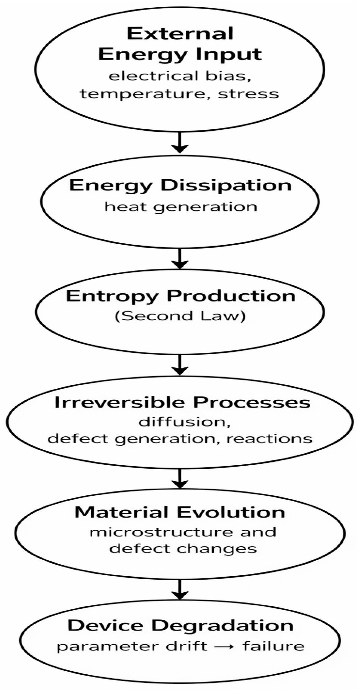
From a reliability perspective, these thermodynamic principles establish the physical basis for gradual degradation under electrical and thermal stress. The cumulative effect of many irreversible microscopic events eventually produces measurable changes in device and circuit parameters. Although the detailed microscopic mechanisms may differ across technologies, the general progression from externally applied stress to defect evolution and macroscopic degradation follows the same thermodynamic framework.

Figure 1 illustrates this general progression schematically, beginning with external stress conditions that drive microscopic defect generation and transport processes, ultimately producing measurable degradation and eventual failure behavior in electronic devices.

2.2. Random Walk and Defect Motion

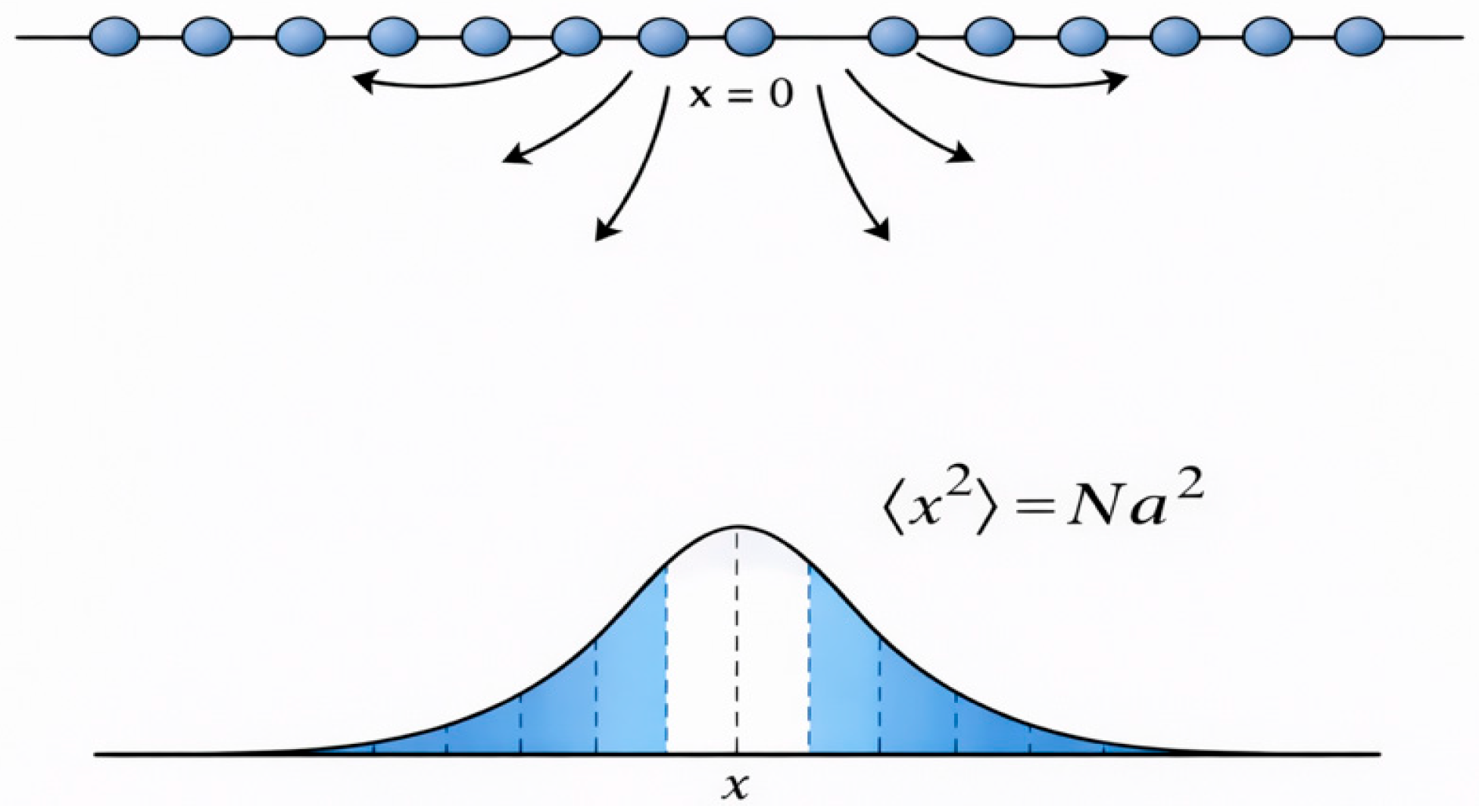
Many degradation processes in electronic materials begin with the motion of atoms, vacancies, ions, or defects within a solid. At finite temperature, atoms vibrate continuously and interact with neighboring atoms. These interactions produce thermally activated particle displacements that, over time, appear as random motion through the lattice. The simplest description of this behavior is the one-dimensional random walk model [1]. In a simple random walk, a particle or defect moves one step either to the left or to the right during each time interval with equal probability. After many steps, the trajectory becomes irregular and unpredictable, as illustrated schematically in Figure 2.

Although the direction of each step is random, the statistical behavior of the ensemble of many particles follows well-defined relations. The average displacement remains zero

$$⟨x⟩=0$$

(5)

while the spread of positions increases with time. The mean square displacement becomes

$$⟨x^2⟩=N{a}^2$$

(6)

where $a$ is the step length and $N$ is the number of steps.

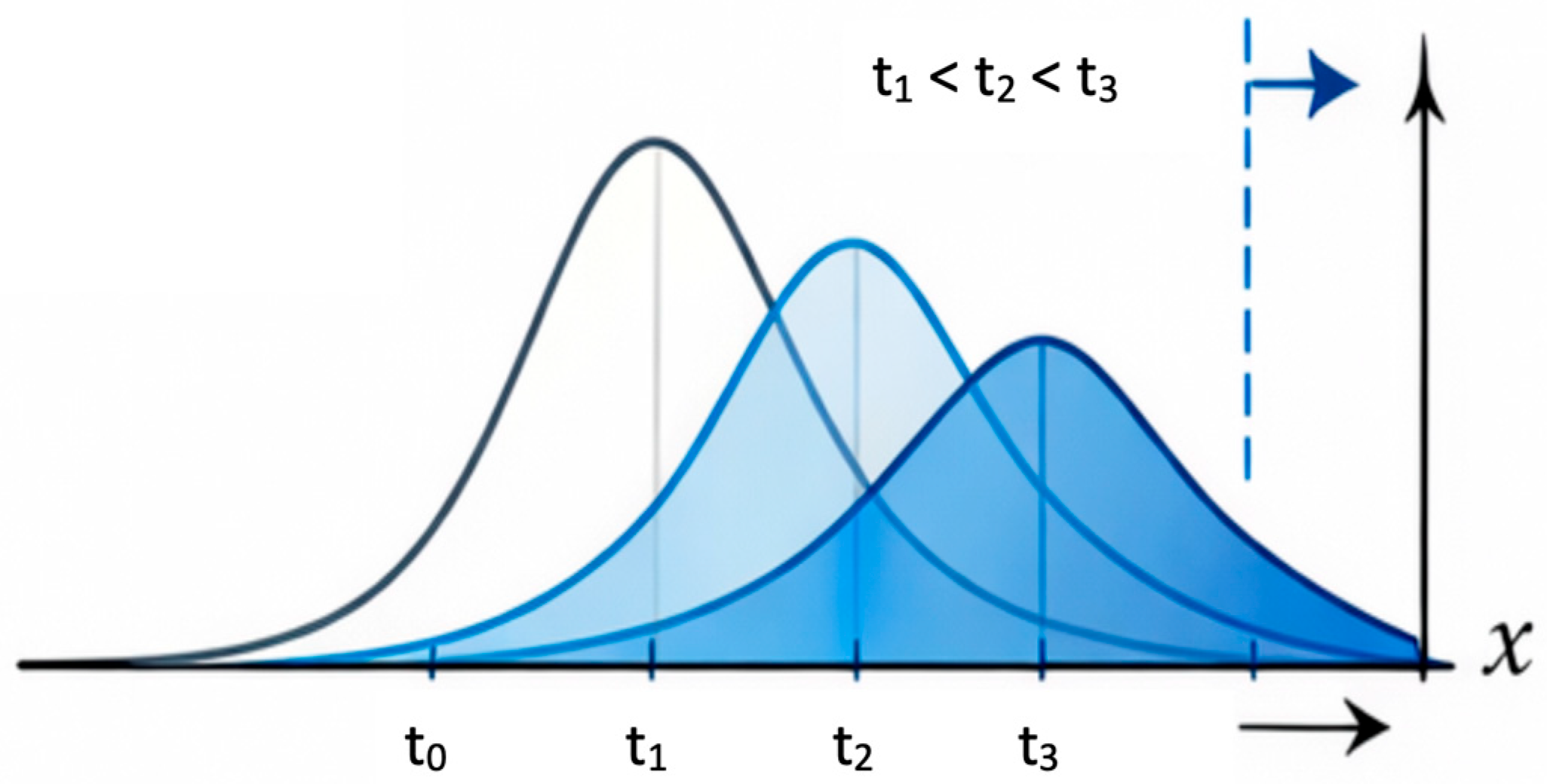
For large numbers of steps, the probability distribution approaches a Gaussian form

$$P\left(x,t\right)={\displaystyle \frac{1}{\sqrt{4\pi Dt}}} \exp \left(-{\displaystyle \frac{x^2}{4Dt}}\right)$$

(7)

where $D$ is the diffusion coefficient. Figure 3 illustrates the broadening of the distribution over time resulting from the diffusive function described by (7) where the peak is reduced by $1/\sqrt{Dt}$ and the lateral extent expands by the same amount preserving the total number of particles or defects.

Random walk motion therefore produces predictable statistical behavior even though the motion of individual particles remains stochastic. In real materials, these random steps correspond to atomic jumps, defect hopping, dislocation motion, ionic transport, or charge migration between localized states.

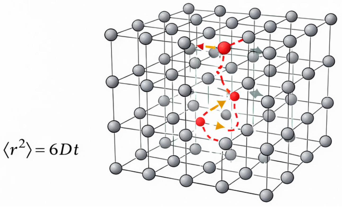
In practical semiconductor devices, defect motion occurs in three dimensions rather than along a single axis. In three dimensions, the mean square displacement becomes

$$⟨r^2⟩=6Dt$$

(8)

which defines the isotropic diffusion in a solid. Figure 4 illustrates this three-dimensional stochastic migration process schematically.

These relations provide the bridge between microscopic stochastic motion and macroscopic transport behavior. Many degradation phenomena in microelectronics, including electromigration, ionic transport, impurity diffusion, and defect motion within gate dielectrics, are governed by these same statistical transport principles.

2.3. Diffusion as the Continuum Limit of Random Transport

The random walk description developed above provides an intuitive microscopic basis for diffusion. For practical reliability modeling, however, it is often more useful to describe transport using continuum concentration equations rather than tracking individual particles.

Let $C\left(x,t\right)$ represent the concentration of mobile species such as vacancies, ions, defects, or reactants. Conservation of particles requires that the local rate of change in concentration be equal the negative divergence of the particle flux $J\left(x,t\right)$:

$${\displaystyle \frac{\partial C}{\partial t}}=-{\displaystyle \frac{\partial J}{\partial x}}$$

(9)

which is the continuity equation. To relate flux (motion) to concentration gradients, Fick’s first law is introduced [2]:

$$J=-D{\displaystyle \frac{\partial C}{\partial x}}$$

(10)

where $D$ is the diffusion coefficient, the same as illustrated in Figure 3 and Figure 4 and Equation (7). Substituting Equation (10) into Equation (9) gives

$${\displaystyle \frac{\partial C}{\partial t}}=-{\displaystyle \frac{\partial }{\partial x}}\left(-D{\displaystyle \frac{\partial C}{\partial x}}\right)$$

(11)

and for the constant diffusion coefficient gives

$${\displaystyle \frac{\partial C}{\partial t}}=D{\displaystyle \frac{{\partial }^{2}C}{\partial x^2}}$$

(12)

which is Fick’s second law.

Equation (12) describes the temporal evolution of concentration profiles under purely stochastic transport. Regions of high concentration gradually spread into neighboring regions of lower concentration, causing initially localized distributions to broaden with time. This behavior follows fundamentally from the second law of thermodynamics and the resulting statistical tendency toward diffusive spreading.

In reliability problems, transport is often influenced not only by random diffusion but also by external driving forces such as electric fields, current flow, or stress gradients. Under these conditions, the total flux contains both diffusive and drift components,

$$J=-D{\displaystyle \frac{\partial C}{\partial x}}+vC$$

(13)

where $v$ is the average drift velocity. Substituting Equation (13) into the continuity equation gives the advection–diffusion equation

$${\displaystyle \frac{\partial C}{\partial t}}=D{\displaystyle \frac{{\partial }^{2}C}{\partial x^2}}-v{\displaystyle \frac{\partial C}{\partial x}}$$

(14)

for constant $D$ and $v$.

The first term describes spreading due to random motion, whereas the second term describes directional transport caused by the applied driving force. In microelectronics reliability, this distinction is important because many degradation mechanisms involve both stochastic broadening and field-driven transport. Examples include electromigration in interconnects, ionic motion in dielectrics, and charged defect migration under gate bias.

The combined action of drift and diffusion therefore provides a direct physical connection between microscopic stochastic motion and the macroscopic transport equations commonly used in degradation modeling. In MOS devices under constant electrical stress, for example, the applied gate voltage introduces a preferred direction for charge transport and defect motion. Under such conditions, degradation may evolve through a combination of random diffusion, directional drift, trapping, and local structural rearrangement.

Although these transport equations arise from relatively simple assumptions, they provide the physical foundation for many reliability models used in practical semiconductor lifetime analysis.

2.4. Energetics of Defect Motion and Arrhenius Kinetics

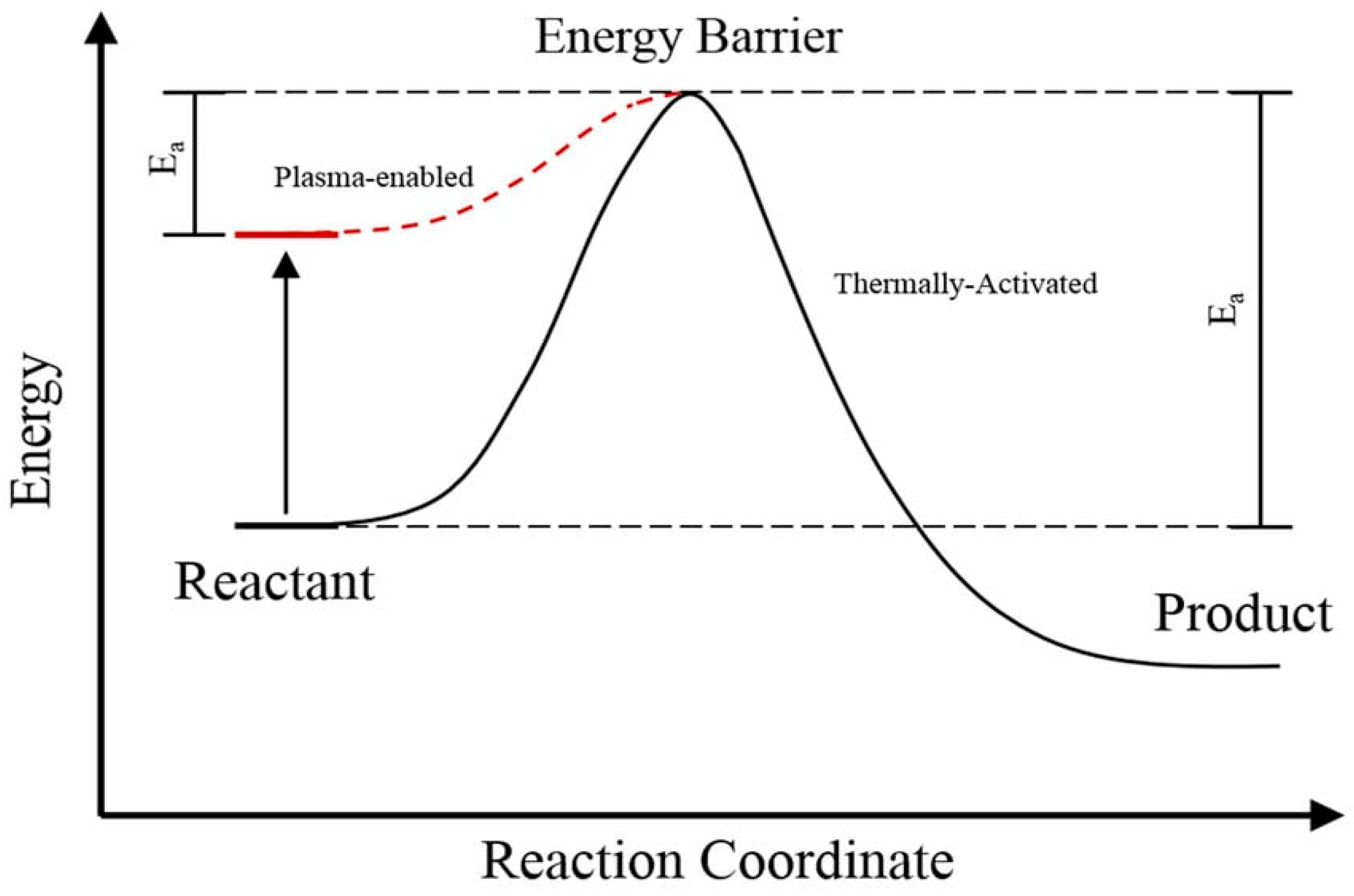
The transport processes described above depend on the ability of atoms, ions, or defects to move between local configurations within a material. Each microscopic transition generally requires overcoming an energy barrier determined by the local atomic structure. The probability of such transitions therefore depends strongly on temperature.

The rate of thermally activated transitions is commonly described by the Arrhenius relation [3]:

$$k=k_0\mathit{exp}\left(-{\displaystyle \frac{E_a}{k_{B}T}}\right)$$

(15)

where $k$ is the transition rate, $k_0$ is an attempt frequency, $E_a$ is the activation energy, $k_B$ is Boltzmann’s constant, and $T$ is the absolute temperature.

Because diffusion results from many such microscopic transitions, the diffusion coefficient also follows an Arrhenius dependence,

$$D=D_0\exp \left(-{\displaystyle \frac{E_a}{k_{B}T}}\right)$$

(16)

where $D_0$ is a prefactor associated with microscopic transport properties. Figure 5 illustrates a simplified energy landscape for a thermally activated transition between two local configurations separated by an activation barrier.

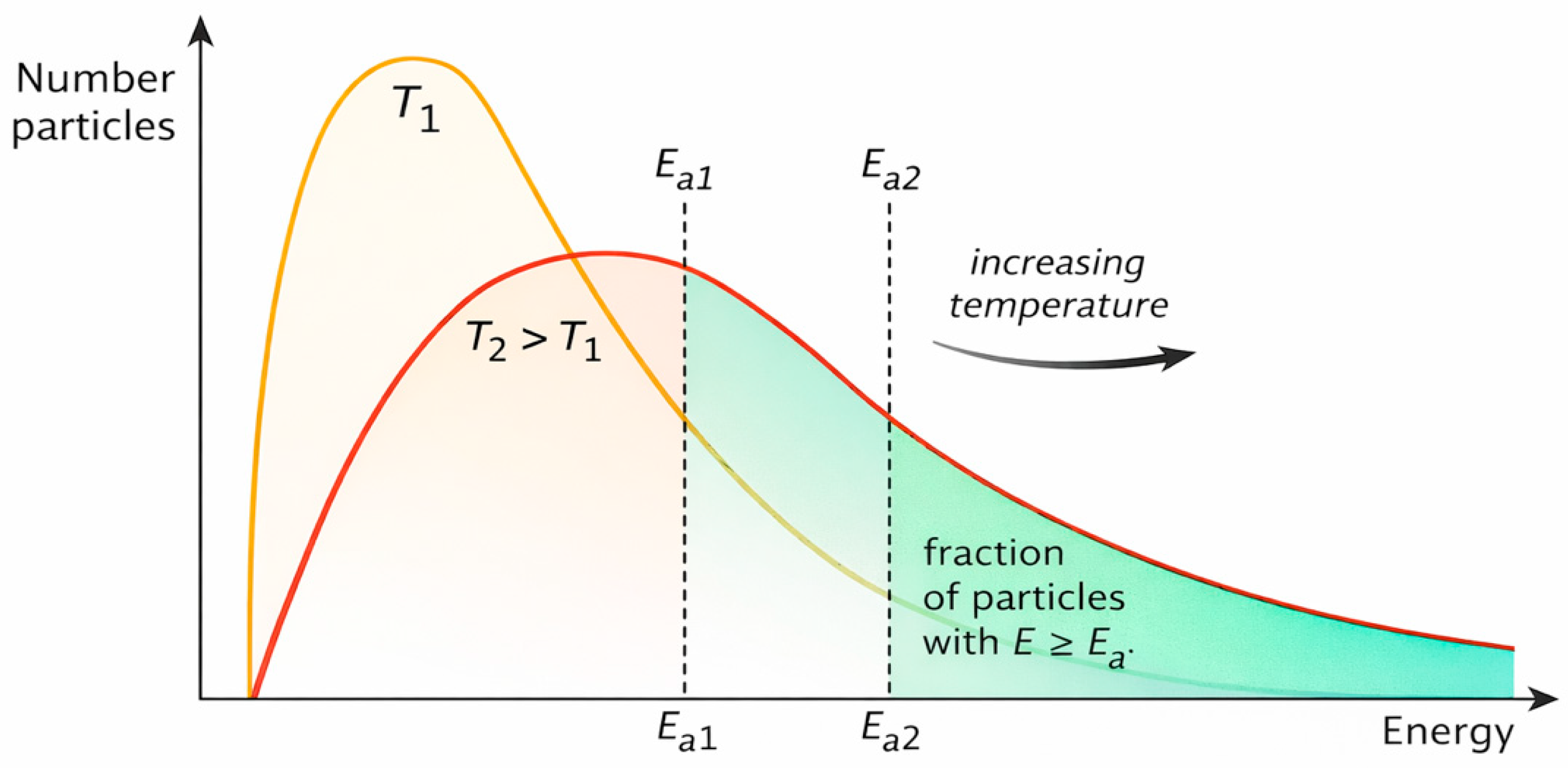
The Arrhenius relation may also be interpreted statistically using the Maxwell–Boltzmann energy distribution. At finite temperature, particles within a material possess a distribution of thermal energies. When this barrier is high, on the order of 0.25 eV or higher for example, only a fraction of particles occupy the high-energy tail of the distribution with sufficient energy to overcome the activation barrier. This is because at room temperature (~300 K) the average thermal energy is about 0.025 eV.

Although electronic solids involve more complicated quantum and collective effects than ideal gases, the Boltzmann factor still provides a useful approximation for describing thermally activated defect processes in many reliability problems. As temperature increases, the fraction of particles capable of overcoming the activation barrier increases exponentially. Figure 6 illustrates this statistical interpretation schematically using the Maxwell–Boltzmann energy distribution.

The characteristic time associated with a thermally activated process is inversely related to the transition rate

$$\tau \propto {\displaystyle \frac{1}{k}}$$

(17)

which gives

$$\tau ={\tau }_0\exp \left({\displaystyle \frac{E_a}{k_{B}T}}\right)$$

(18)

where ${\tau }_0$ is a prefactor related to the inverse attempt frequency.

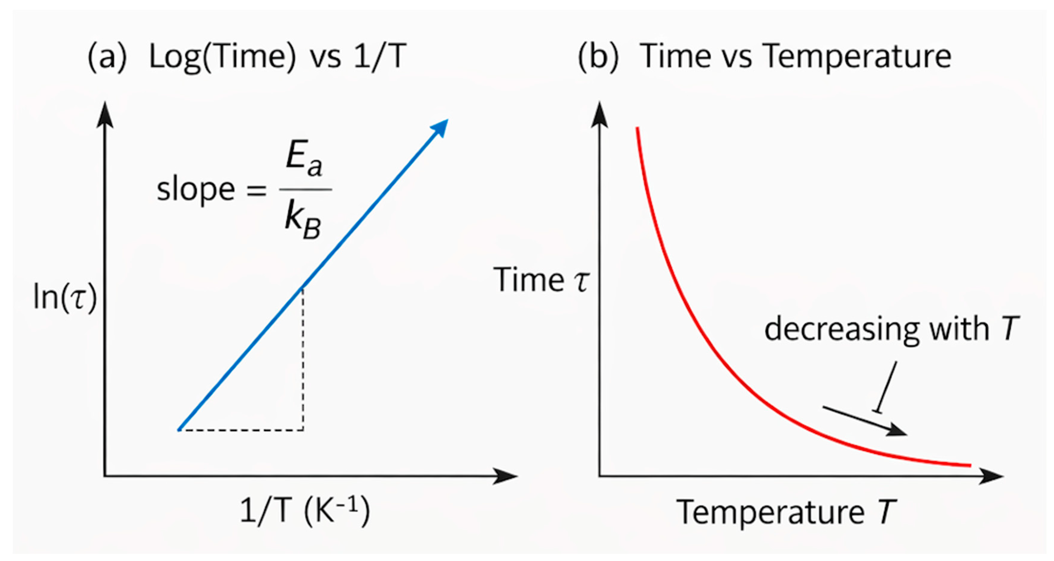
This relation forms the basis for accelerated reliability testing. Devices are stressed at elevated temperatures in order to accelerate degradation and observe measurable parameter changes within practical laboratory time scales. When characteristic degradation times are plotted as a function of inverse temperature, thermally activated processes often exhibit approximately linear Arrhenius behavior. Figure 7 illustrates this commonly used Arrhenius representation.

The thermally activated process framework developed in this section thus provides the microscopic kinetic basis for many reliability acceleration models used in semiconductor lifetime prediction. At the same time, experimentally observed degradation behavior often exhibits smoother empirical scaling behavior extending over many decades in time. The following sections examine how such empirical relations emerge from the collective behavior of many microscopic stochastic processes and how they are interpreted in practical reliability analysis.

3. Thermally Activated Kinetics and Reliability Scaling

The thermodynamic and transport processes described in Section 2 provide the microscopic basis for degradation in electronic materials and devices. In practical reliability experiments, however, individual microscopic transitions are not directly observed. Instead, measurements typically monitor cumulative macroscopic properties such as threshold voltage shift, resistance increase, leakage current, interface-state density, or transconductance degradation. These measurable quantities reflect the collective behavior of a broad variety of stochastic microscopic processes evolving simultaneously under electrical and thermal stress and each often with its own activation energy and related kinetic properties.

The transition rates introduced in Equations (15)–(18) determine the probability and time scale of microscopic defect motion and reaction processes. In realistic materials, however, degradation rarely proceeds through a single isolated activation barrier or a single deterministic pathway. Semiconductor devices contain distributions of dopants, defects, local strain variations, interfaces, grain boundaries, and metastable trapping states. As a result, degradation commonly occurs through the collective interaction of many microscopic processes over a broad range of time scales.

In many reliability experiments, the cumulative effect of these stochastic processes produces smooth empirical degradation behavior extending over many decades in time. One commonly observed form is a sublinear power-law dependence:

$$\mathsf{\Delta }P\left(t\right)=A{t}^n$$

(19)

where $\mathsf{\Delta }P$ represents a measurable degradation parameter, $A$ is a stress-dependent prefactor, and $n$ is the time exponent. In many experimentally observed systems, the exponent satisfies the sublinear condition, namely

$$0<n<1$$

(20)

corresponding to degradation that slows progressively with time [32].

Power-law behavior does not imply that every microscopic process itself follows an explicit power-law transition probability. Rather, such behavior may emerge statistically when many interacting stochastic processes evolve collectively over broad temporal and energetic distributions. Distributed activation energies, dispersive transport, defect interaction, electrostatic screening, and trapping-limited kinetics can all contribute to effective sublinear macroscopic degradation behavior. Similar empirical scaling relations also appear in fatigue, diffusion-limited growth, dielectric degradation, and electromigration phenomena for just a few examples [4,5,6].

One possible physical interpretation of sublinear degradation is that the degradation rate decreases as the system evolves. This behavior may be described phenomenologically by

$${\displaystyle \frac{d\left(\mathsf{\Delta }P\right)}{dt}}\propto {\displaystyle \frac{1}{{\left(\mathsf{\Delta }P\right)}^{m-1}}}$$

(21)

where

$$m={\displaystyle \frac{1}{n}}$$

(22)

so that integrating Equation (21) produces the power-law relation of Equation (19). Physically, this behavior corresponds to degradation processes that progressively slow as defects accumulate, local energetic configurations evolve, or accessible states become increasingly screened or stabilized.

The reciprocal exponent $m$ directly characterizes the degree of nonlinearity in the degradation kinetics. More generally, $m$ describes the feedback between accumulated degradation and the subsequent degradation rate. For $m=1$, the degradation rate becomes independent of the accumulated degradation and the parameter evolves linearly with time. For $m>1$, degradation progressively slows as degradation accumulates, consistent with retarding processes in which existing degradation suppresses further degradation. Examples may include trapping, screening, site depletion, or other mechanisms that reduce the availability of energetically favorable degradation pathways. In contrast, for $0<m<1$, the degradation rate increases as degradation accumulates, corresponding to accelerating or cooperative processes in which existing damage promotes additional degradation. Thus, the exponent $m$ provides a quantitative measure of the interaction between accumulated degradation and the subsequent degradation kinetics.

In many semiconductor degradation mechanisms, the experimentally observed exponent satisfies $m>1$, indicating degradation processes that progressively retard with time. In bias temperature instability (BTI), for example, threshold-voltage degradation commonly follows sublinear power-law kinetics extending over many decades in time [7,8,9,10,11,12,13,14,15,16,21,22,23,24,25,26,27,28,29,30,31]. Similar behavior has been reported in wide-bandgap devices, dielectric degradation, and interface-state evolution. These observations suggest that the degradation rate often decreases as degradation accumulates, even though the underlying microscopic mechanisms may differ substantially among technologies and materials systems.

The empirical form of Equation (19) therefore provides a useful macroscopic description of degradation kinetics even when the detailed microscopic interactions remain complex. At the same time, the parameters appearing in Equation (19) often exhibit systematic dependence on electrical and thermal stress conditions. In practical reliability analysis, understanding this stress dependence becomes essential for meaningful lifetime extrapolation. Because experimentally measured degradation parameters are typically extracted from differential quantities near the measurement floor, interpretation of empirical power-law behavior may become highly sensitive to experimental uncertainty. This effect is often amplified by logarithmic representation. The following sections therefore examine practical issues associated with degradation interpretation, exponent extraction, and reliability extrapolation.

4. Interpretation of Power-Law Degradation Measurements

Equation (19) is widely used to analyze experimentally observed degradation behavior in semiconductor reliability studies. In practice, however, the interpretation of empirical power-law degradation involves several important experimental and mathematical subtleties that are often overlooked during conventional log–log analysis.

Measured degradation parameters are generally not absolute quantities. Instead, degradation is typically determined as the difference between a measurement in time of some parameter and an initial reference value

$$\mathsf{\Delta }P=P-P_0$$

(23)

where $P_0$ is the initial reference parameter and $P$ is the measured value over time. Examples include threshold voltage shift, resistance increase, leakage-current variation, or interface-state generation.

Even if the initial reference value were assumed perfectly known, which is itself unrealistic due to the natural measurement error of the system, the stressed measurement still contains finite experimental uncertainty:

$$P=P_{true}\pm {\sigma }_P.$$

(24)

As a result, small degradation values near the measurement floor inherently contain large relative uncertainty. More generally, when uncertainty exists in both the assumed initial measurements and the monitored parameter, standard propagation of uncertainty gives

$${\sigma }_{\mathsf{\Delta }P}=\sqrt{{\sigma }_P^2+{\sigma }_{P_0}^2}$$

(25)

showing that the uncertainty in the differential quantity remains finite even as $\mathsf{\Delta }P$ approaches zero.

This issue becomes particularly important in logarithmic representations commonly used for power-law extraction. Conventional analysis frequently applies a logarithmic transformation to Equation (19), resulting in the following equation:

$$\log \left(\mathsf{\Delta }P\right)=\log \left(A\right)+n\log \left(t\right)$$

(26)

and then extracts the time exponent from the slope of the resulting linear fit. However, the logarithm becomes increasingly unstable as $\mathsf{\Delta }P$ approaches the measurement floor, where the noise will inherently go negative simply due to the uncertainty ${\sigma }_{\mathsf{\Delta }P}$. Because experimental uncertainty remains finite while the measured degradation approaches zero, the relative uncertainty

$${\displaystyle \frac{{\sigma }_{\mathsf{\Delta }P}}{\mathsf{\Delta }P}}$$

(27)

diverges as

$$\mathsf{\Delta }P\to 0$$

(28)

Under such conditions, small fluctuations in the measured parameter produce disproportionately large variations in the logarithmic representation. In practice, degradation values near the noise floor may fluctuate around zero, causing the logarithm to become undefined for negative excursions and highly unstable for small positive values. This will create a challenge even finding the initial reference parameter $P_0$.

Consequently, the earliest portions of degradation datasets often become highly sensitive to this baseline definition, $P_0$, as well as the relative measurement uncertainty and experimental noise. Reliable logarithmic fitting therefore requires that the degradation values are substantially larger than the effective measurement uncertainty. This requirement can systematically exclude early-time data and distort the apparent curvature and the measured slope, n, of the power-law representation of the data.

These effects become particularly important at lower stress conditions where degradation evolves more slowly and remains near the measurement floor for longer periods of time. Under such conditions, the apparent curvature observed in conventional log–log representations may reflect the combined effects of baseline uncertainty and logarithmic instability rather than intrinsic changes in the underlying degradation physics. 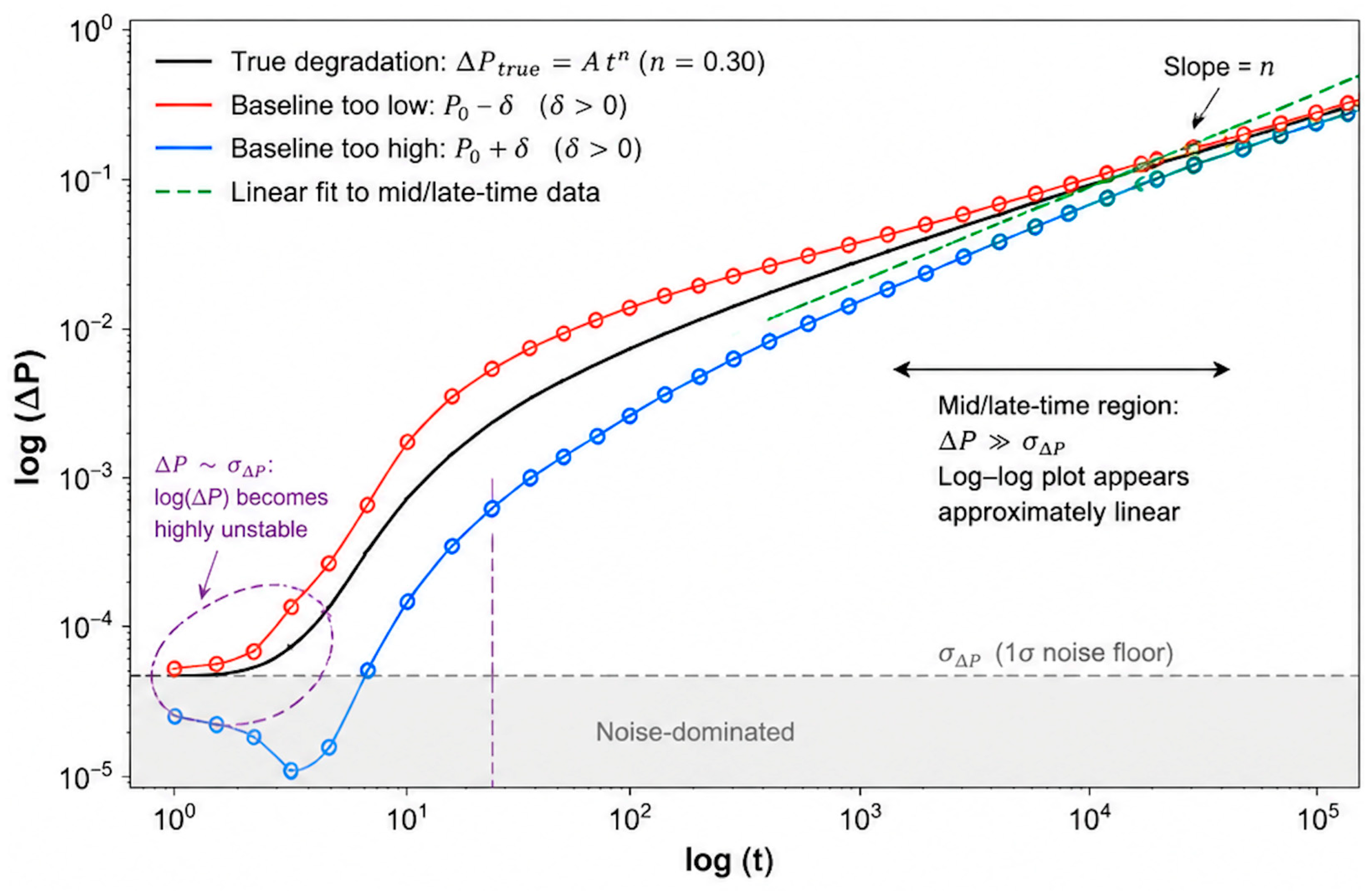Figure 8 schematically illustrates how small baseline uncertainty due to measurement noise ${\sigma }_{\mathsf{\Delta }P}$ near the measurement floor can produce systematic curvature in logarithmic degradation trajectories and errors in the extrapolated slope, n [27].

Conventional goodness-of-fit metrics may not reliably detect this problem. In many cases, log–log degradation trajectories may exhibit very high linear correlation coefficients giving a false sense of confidence in the fit, even when systematic curvature remains present in the residual structure. This distinction is important because conventional least-squares fitting primarily measures overall variance reduction rather than the absence of systematic curvature. As a result, apparently excellent linear fits may still produce significant errors in extracted exponents and long-term lifetime extrapolation when projected across many decades in time. These observations motivate the need for extraction procedures that explicitly account for baseline sensitivity and geometric curvature during power-law interpretation [27].

5. Baseline-Independent Linearization and Exponent Extraction

The logarithmic instability discussed in Section 4 calls out a need for an extraction method that is less sensitive to baseline uncertainty and systematic curvature. In conventional log–log analysis, degradation trajectories are interpreted directly from Equation (26) using linear regression in logarithmic coordinates. However, as we see, this representation may be highly sensitive to early-time uncertainty and geometric distortion near the measurement floor.

One approach to reducing this sensitivity is to transform the time axis alone, rather than applying a logarithmic transformation to the measured parameter. Starting from the power-law relation of Equation (19), $\mathsf{\Delta }P\left(t\right)=A{t}^n$, the relation may be rewritten as

$$\mathsf{\Delta }P\left(t\right)=Ax$$

(29)

using the transformed variable

$$x=t^n=t^{1/m}.$$

(30)

The data is then fit to the proper exponent causing the degradation trajectory to become geometrically linear under the transformed x coordinate. Rather than fitting only a straight line, the transformed representation may be fit to a second-order polynomial,

$$\mathsf{\Delta }P=a{x}^2+bx+c$$

(31)

where the quadratic coefficient $a$ directly measures residual curvature in the transformed trajectory.

This distinction is important because conventional goodness-of-fit metrics alone may fail to detect systematic curvature. A dataset may exhibit an extremely high $R^2$ value while still containing an incorrect global form that could lead to a large discrepancy in extrapolated time to failure. For example, degradation points may systematically fall below the fitted line at early times, above the line at intermediate times, and below again at long times. Such residual structure could indicate systematic curvature even when the overall linear correlation remains extremely high.

The quadratic coefficient in Equation (31) therefore provides a direct measure of residual curvature rather than simply overall variance reduction. Under the correctly transformed exponent, the quadratic term approaches zero and the degradation trajectory becomes maximally linearized over the full experimental time range. This procedure is explained in more detail in Bernstein [27].

This systematic curvature becomes particularly important at lower stress conditions where degradation evolves slowly and early-time measurements remain near the effective noise floor. Also, early times of lifetime experiments is when the apparatus usually is not completely stabilized. Under such conditions, baseline uncertainty and logarithmic instability may produce subtle curvature that strongly distorts conventional exponent extraction in the long term. The transformed representation of (31) reduces this measurement sensitivity by avoiding direct logarithmic amplification of small differential quantities.

The extracted exponent also plays a central role in practical lifetime extrapolation. For a failure criterion defined as the critical degradation $\mathsf{\Delta }{P}_{crit}$, Equation (19) gives

$$\mathsf{\Delta }{P}_{crit}=A\left(V,T\right)TT{F}^n$$

(32)

which may be rearranged as

$$TTF={\left({\displaystyle \frac{\mathsf{\Delta }{P}_{crit}}{A(V,T)}}\right)}^{1/n}$$

(33)

or equivalently as

$$TTF={\left({\displaystyle \frac{\mathsf{\Delta }{P}_{crit}}{A(V,T)}}\right)}^m.$$

(34)

Equation (34) demonstrates that the reciprocal exponent $m$ geometrically amplifies voltage and temperature acceleration during lifetime extrapolation. Consequently, relatively small changes in the extracted exponent may produce orders-of-magnitude differences in projected lifetime.

This effect may also strongly influence apparent activation energies extracted from conventional Arrhenius analysis. If a conventional extraction produces an apparent activation energy of

$$E_{a,app}=0.5\mathrm{eV}$$

(35)

while the measured degradation follows

$$n=0.2,\left(m=5\right)$$

(36)

then the intrinsic activation barrier associated with the prefactor $A\left(V,T\right)$ may instead correspond approximately to

$$E_{a,true}=n{E}_{a,app}=0.1\mathrm{eV}$$

(37)

This result suggests that much of the apparent stress acceleration observed in conventional lifetime extraction may arise from geometric amplification through the exponent rather than exclusively from large intrinsic activation barriers. Physically, such behavior may indicate degradation dominated by occupation and evolution of pre-existing localized states rather than repeated rupture of high-energy chemical bonds. The transformed lifetime quantity

$$TT{F}^n\propto {\displaystyle \frac{1}{A(V,T)}}$$

(38)

therefore, separates intrinsic stress acceleration from exponent-driven geometric amplification and provides a more direct representation of the underlying degradation prefactor.

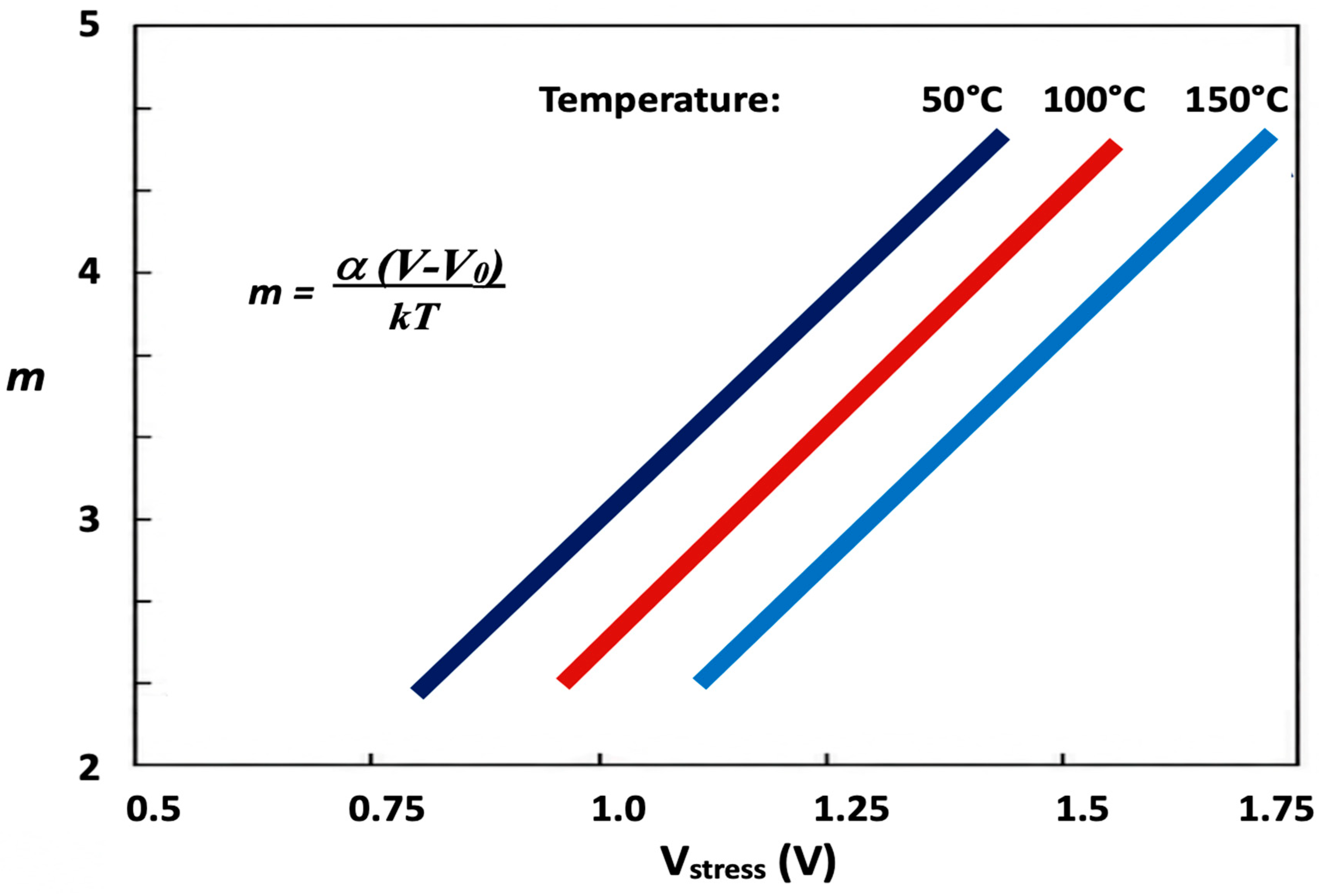
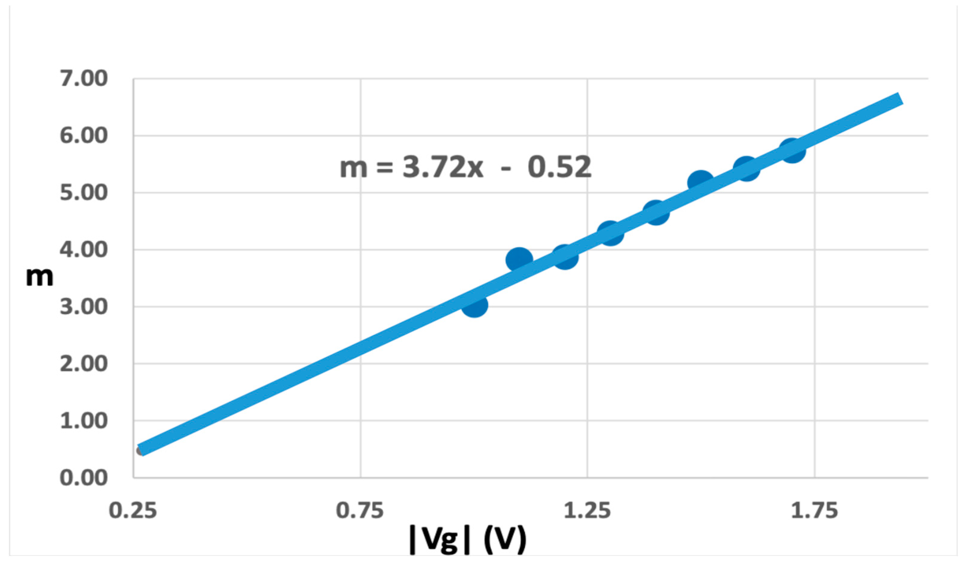
For analytical convenience, it is often useful to express the power-law exponent in terms of the reciprocal quantity $m={\displaystyle \frac{1}{n}},$ so that the degradation relation may be written as $\mathsf{\Delta }P\left(t\right)=A{t}^{1/m}.$ When expressed in this form, the dependence of the exponent on stress voltage can often be approximated by a simple linear relation over the range of experimentally relevant conditions. Stress-dependent exponent behavior is often observed systematically across voltage ranges. An example of this behavior is shown in Figure 9, where the extracted parameter $m$ increases approximately linearly with the magnitude of the applied gate voltage [33].

The stress dependence of the exponent shown here is not limited to voltage effects. Experimental studies have also shown that the power-law exponent varies with temperature, reflecting the influence of thermally activated transport and reaction processes on the underlying degradation kinetics [10]. Figure 10 illustrates an example in which the measured inverse power law exponent, $m={\displaystyle \frac{1}{n}}$, increases with temperature when plotted as a function of V_stress, and temperature T. We see from [10,33] that there is a uniform dependence with 1/kT, expressed as

$$m\left(V,T\right)=\alpha {\displaystyle \frac{V-V_0}{kT}}$$

(39)

where V₀ represents some zero stress offset and $\mathsf{\alpha }~0.1{\displaystyle \raisebox{1ex}{$°\mathrm{C}$}\!\left/ \!\raisebox{-1ex}{$\mathrm{V}$}\right.}$ [33].

These observations demonstrate that the empirical power-law exponent is itself a stress-dependent parameter. As a result, the apparent TTF relations derived from degradation measurements may exhibit nonlinear behavior even when the underlying acceleration physics remains relatively simple.

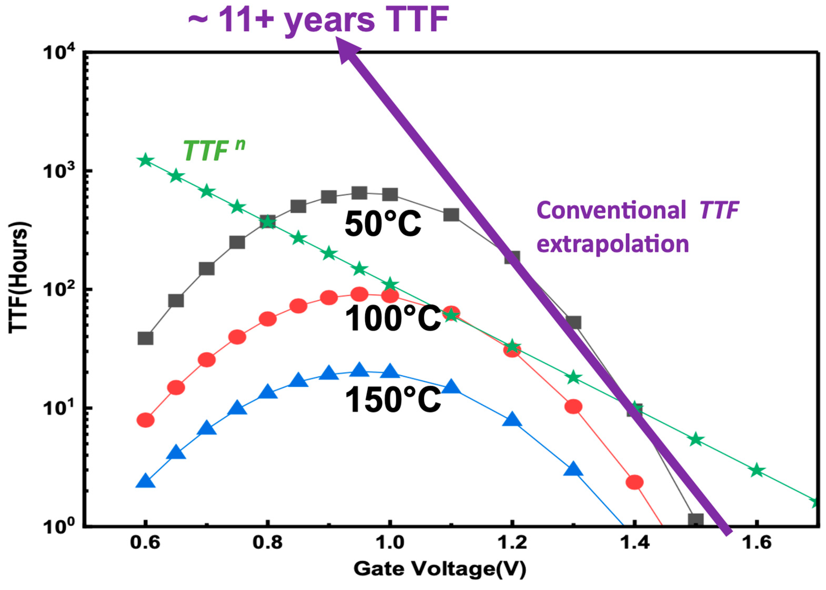
The influence of exponent variation on lifetime extrapolation is illustrated in Figure 11, which shows predicted time-to-failure values as a function of stress voltage [12]. When the lifetime is plotted directly as $TTF$, the resulting curves exhibit pronounced curvature because the exponent changes with voltage. However, when the transformed quantity ${TTF}^n$ as derived from Equation (17) is plotted instead, the relation becomes linear, revealing the true underlying stress acceleration behavior [5]. The purple line illustrates the conventional extrapolation approach which can lead to an >11-year expected TTF.

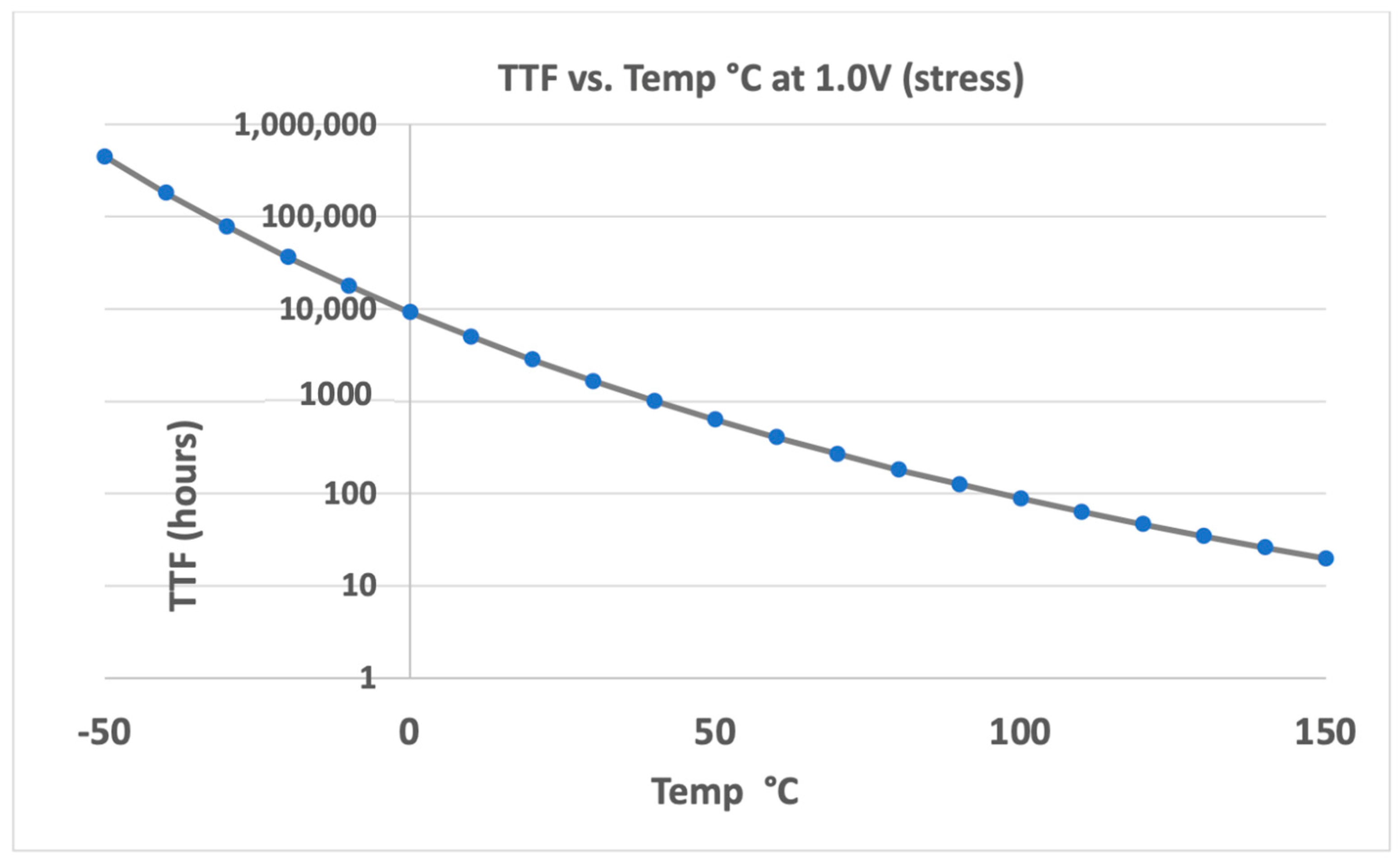
A similar effect appears in temperature acceleration experiments. Figure 12 shows an example of TTF values plotted as a function of temperature at fixed stress voltage. The apparent curvature of the lifetime relation arises from the combined effects of thermally activated degradation processes and the temperature dependence of the time exponent.

Together, these observations illustrate an important principle in reliability analysis. We see that the chosen form of test plotting axes can strongly influence the interpretation of the extrapolated TTF. We see how important it is to evaluate properly the time dependence due to the degradation kinetics. When degradation follows a power-law relation with a stress-dependent exponent, transformations such as $TT{F}^n$ can provide a more direct representation of the underlying degradation physics. Thus, proper extraction of the time dependence represented by $n=1/m$ becomes critical for meaningful lifetime extrapolation.

6. Conclusions

Reliability degradation in modern semiconductor technologies emerges from the cumulative effect of many microscopic stochastic processes evolving under electrical, thermal, and mechanical stress. Defect motion, diffusion, trapping, atomic rearrangement, and thermally activated transitions occur at the microscopic scale, yet experimental degradation measurements frequently exhibit smooth macroscopic empirical behavior extending across many decades in time. Understanding the relationship between these microscopic physical processes and the empirical methods used for practical reliability analysis remains an important challenge in microelectronics reliability engineering.

This tutorial reviewed the thermodynamic and kinetic foundations underlying degradation phenomena in electronic materials and devices. Random walk, diffusion, irreversible thermodynamics, and Arrhenius kinetics were introduced as the microscopic basis for defect evolution and transport. The discussion here then examined how collective stochastic processes can produce smooth empirical scaling relations, particularly sublinear power-law degradation behavior commonly observed in semiconductor reliability experiments.

Attention was given to the interpretation of empirical power-law kinetics and their role in accelerated lifetime extrapolation. Experimental observations increasingly indicate that degradation exponents may depend systematically on stress conditions such as voltage and temperature. Under such conditions, lifetime projections become highly sensitive to the extraction and interpretation of the time exponent. The reciprocal exponent $m=1/n$ was shown to amplify geometrically stress acceleration during time-to-failure (TTF) extrapolation, potentially producing large differences in projected lifetime even for relatively small changes in the extracted exponent.

The tutorial also examined important practical limitations associated with conventional logarithmic degradation analysis. Because experimentally measured degradation quantities are differential parameters extracted near the measurement floor, logarithmic representations may become highly sensitive to baseline uncertainty and experimental noise. Under these conditions, apparently excellent linear fits may still contain systematic curvature capable of significantly distorting extracted degradation exponents and long-term lifetime projections. These observations motivate a demonstrated extraction procedures that explicitly evaluates residual curvature and geometric consistency rather than relying solely on conventional goodness-of-fit metrics.

A transformed-coordinate linearization methodology was therefore discussed in which degradation trajectories are evaluated directly in $t^{1/m}$ coordinates using curvature-sensitive polynomial fitting. This approach reduces sensitivity to logarithmic instability near small degradation values and provides a more direct framework for interpreting stress-dependent degradation kinetics and TTF calculation.

The purpose of this tutorial is not to propose a single universal degradation mechanism or universal reliability law. Rather, the goal is to provide a unified conceptual framework connecting microscopic stochastic degradation physics with the empirical analysis methods widely used in practical reliability engineering. As semiconductor technologies continue to evolve toward increasingly complex materials, interfaces, and device architectures, careful interpretation of degradation measurements and accelerated lifetime extrapolation will remain essential for meaningful reliability prediction.

7. Key Takeaways

The key takeaways of this study are as follows:

• Microscopic degradation processes originate from thermally activated events. Defect motion, charge trapping, and bond rearrangement occur through stochastic transitions governed by statistical mechanics and transport processes such as diffusion.
• Macroscopic degradation behavior often appears as empirical scaling relations. Although the underlying microscopic dynamics may be complex, many reliability phenomena exhibit smooth power-law time dependences over extended time ranges.
• Power-law degradation provides a practical bridge between physics and reliability engineering. Relations of the form $\mathsf{\Delta }P\left(t\right)=A{t}^n$ allow degradation measurements obtained during accelerated testing to be interpreted within a framework consistent with thermally activated kinetics.
• The power-law time exponent is often stress dependent. Experimental studies of phenomena such as bias temperature instability show that the exponent $n$ can vary with voltage, temperature, and device structure, reflecting changes in the underlying degradation dynamics.
• Time-to-failure projections are sensitive to the time exponent. Because reliability projections typically require extrapolation over many decades of time, small variations in the exponent can significantly affect predicted device lifetimes.
• Appropriate transformations can clarify stress acceleration behavior. When degradation follows a power-law relation, representations such as $TT{F}^n$ can reveal exponential stress dependences that may appear nonlinear in conventional $TTF$ plots.
• Combining physics-of-failure and empirical reliability approaches provides the most effective interpretation of degradation measurements. Physical insight helps explain observed trends, while empirical relations provide practical tools for analyzing complex systems and projecting long-term device behavior.