Use of Machine Learning to Predict the Performance of Tile Adhesive Mortars

Abstract

Tile adhesive mortars are industrialized products used for installing ceramic coverings and are classified according to the Brazilian standard ABNT NBR 14081/2012 on the basis of tensile adhesion performance under different curing conditions. Their formulation directly affects both technical performance and manufacturing competitiveness, while conventional product development remains slow, costly and strongly dependent on trial-and-error laboratory testing. This study evaluates whether historical industrial formulation data can support the retrospective prediction of approval or failure of tile adhesive mortars under ambient, oven, immersed and open-time curing conditions. A dataset comprising 6031 individual pull-off observations collected between 2021 and 2023 by a European multinational company in the construction materials sector was used to train and compare Logistic Regression, Random Forest, Boosted Decision Tree and Support Vector Machine models in R and Azure. The study was designed as an industrial-data modelling investigation rather than as a prospective optimization experiment. The results show that ensemble tree-based models, particularly Boosted Decision Tree and Random Forest, achieved the strongest predictive performance, whereas Logistic Regression remained more suitable for inferential interpretation of formulation variables. Model performance was uneven across curing conditions: prediction was more reliable for oven and immersed curing, whereas ambient curing and open time were affected by strong class imbalance and low failure prevalence. The findings indicate that Machine Learning can support formulation screening and quality-oriented decision-making for tile adhesive mortars, provided that its use remains restricted to the formulation ranges represented in the historical dataset and is complemented by prospective experimental validation before deployment in new product development.

1. Introduction

Mortars are construction materials used in various stages of a building project: for laying bricks, for flooring and wall coverings, as adhesive and grout for ceramic pieces, and even for finishing and decorating walls and ceilings. They are composed mainly of a binder (such as cement and lime), fine aggregates (such as sand and ground limestone), water, and may also contain specific chemical additives. Since their applications are very different, for the mortar to meet the necessary requirements for each use, its composition must also vary and be adapted to each case [1].

Tile adhesive mortars are industrialized products specifically designed for installing ceramic coverings (such as tiles and porcelain tiles) on floors and walls. They are sold as a bagged powder composed of cement, sand, and chemical additives that, when mixed with water, form a viscous, plastic, and adhesive paste. These mortars need to be capable of bonding tiles of different sizes under various conditions (indoor environments, outdoors, swimming pools, and building facades) and are usually applied in a thin layer, no thicker than 20 mm, directly over concrete or over existing flooring [2,3].

The Brazilian standard ABNT NBR 14081/2012 [4] classifies tile adhesive mortars into three main types according to their performance: AC-I, AC-II, and AC-III. Performance is evaluated through the tensile adhesion strength test, which measures the force required to detach a ceramic tile bonded to a standard substrate with the tested mortar after 28 days of curing under specific conditions. Formulation is a determining factor both for the performance of the mortars and for the competitiveness of the company that manufactures and markets these products, since their final cost is strongly dependent on the cost and proportion of the raw materials used [2,3].

The development of new formulations for tile adhesive mortars, or the optimization and correction of existing ones, is a lengthy, complex and high-cost process. It is generally based on the theoretical and practical experience of the formulator, and trial-and-error methods are used to arrive at the final recipe. Moreover, tensile adhesion results are only available after the curing period required by the standard, and they are rarely satisfactory on the first attempt. In an effort to shorten development time, several formulations are typically created for each product in each test round, resulting in a high volume of laboratory tests and not necessarily yielding an optimized recipe by the end of the process [5,6,7]. This creates a practical need for data-driven tools capable of screening formulations before additional laboratory campaigns are undertaken.

Machine Learning is a field of Artificial Intelligence that aims to develop computational algorithms capable of learning or identifying patterns from a dataset autonomously—that is, without having been explicitly programmed to do so [8]. Machine Learning algorithms are classified into two main types: (1) Supervised Models, which aim to predict the outcome of a target variable based on input variables, and (2) Unsupervised Models, which aim to identify patterns and relationships within the data in order to group them [9].

Different Machine Learning techniques have been used in recent years to predict the performance of cement-based materials based on formulation and curing variables. Most studies focus on concrete and generally aim to predict compressive strength, tensile strength, durability indicators, sustainability metrics or mixture optimization targets [5,9,10,11,12,13,14,15,16,17,18,19,20,21,22,23,24,25,26,27,28,29,30]. Although this literature provides an important methodological foundation, it cannot be transferred mechanically to tile adhesive mortars. Concrete performance is usually evaluated through bulk mechanical behaviour, whereas tile adhesive mortars are assessed through adhesion to a substrate, pull-off strength, open time and performance under specific normative curing conditions. In these materials, cellulose ether, redispersible polymers, water retention, workability, substrate interaction and curing history play a more central role than in conventional concrete mixture design [2,6,16,23,24].

Studies focused on predicting the properties of tile adhesive mortars based on formulation remain comparatively scarce. Earlier works used statistical mixture design to model formulation–performance relationships [6,7,16]. More recent studies have begun to apply Artificial Intelligence, multiscale modelling or Machine Learning to cementitious tile adhesives and related mortar applications, but these studies are generally based on controlled experimental mixtures, limited datasets, compressive or tensile strength prediction, or optimization-oriented frameworks rather than retrospective classification of standard approval across multiple curing conditions [23,24,30]. Therefore, a relevant gap remains: whether historical industrial data, collected during routine product development rather than through a planned factorial experiment, can be used to train classification models capable of supporting formulation screening for tile adhesive mortars.

The positioning of the present study in relation to previous formulation–performance studies is summarized in

Table 1. Positioning of the present study in relation to previous formulation–performance studies on tile adhesive mortars and related cementitious materials.

Aspect	Previous Adhesive-Mortar Studies	Recent AI/ML Studies in Cementitious Materials	Present Study
Data source	Mostly controlled mixture-design experiments or literature datasets	Concrete, mortar or cementitious datasets, often designed for strength or optimization	Historical industrial records collected during routine product development
Main target	Specific formulation–property relationships	Compressive/tensile strength, sustainability or multi-objective optimization	Approval/failure classification under four ABNT curing conditions
Methodological focus	Statistical mixture design, PCA or regression-type modelling	Ensemble models, neural networks, explainability and optimization	Comparison of classification models and inferential interpretation of formulation variables
Contribution	Useful for planned experiments but less suited to unplanned historical datasets	Shows broader feasibility of data-driven materials design	Tests whether retrospective industrial data can support formulation screening for tile adhesive mortars

Note: Any background shading in Table 1 is used only to distinguish table columns and has no analytical meaning.

.

A European multinational company in the construction materials sector holds an extensive database containing the testing history from the development of tile adhesive mortars. Therefore, it is relevant to explore whether such a dataset can be used to train Machine Learning models capable of predicting whether a formulation is likely to pass or fail the performance requirements defined by the standard. This study should be understood as a retrospective industrial-data modelling study, not as a prospective experimental optimization campaign. A specific subset of the database was used, comprising experimental results obtained between 2021 and the first quarter of 2023 for AC-II and AC-III type mortars, to train different models with three objectives:

• Predictive: to predict whether a given formulation will pass or fail a curing test in accordance with the tile adhesive mortar standard for AC-II or AC-III types.
• Inferential: to determine which variables are most important for predicting approval in each curing condition according to the standard, and to understand how each of them influences this prediction.
• Comparative: to compare the different models obtained for each curing condition in terms of their predictive and inferential capabilities.

2. Materials and Methods

This section is divided into two main subsections: (1) presentation of the tile adhesive mortars, the method used to evaluate their performance, and the main raw materials used in their production; and (2) presentation of the database and the methodology used to train the Machine Learning models.

2.1. Tile Adhesive Mortars

The Brazilian standard ABNT NBR 14081/2012 [4] classifies tile adhesive mortars into three main types according to their performance: AC-I is the most basic mortar, recommended only for indoor use; AC-II is a mortar with intermediate performance, suitable for both indoor and outdoor environments; whereas AC-III offers higher performance, also suitable for indoor and outdoor use, but with superior adhesion compared to types I and II. Approval thresholds for tensile adhesion strength defined by the standard are 0.5 MPa for AC-II across all curing conditions; 1.0 MPa for AC-III under normal, immersed and oven curing; and 0.5 MPa for AC-III under the open-time test. AC-I is not evaluated under oven curing.

The performance of tile adhesive mortars is evaluated through the tensile adhesion strength test, which measures the force required to detach a ceramic tile bonded to a standard substrate using the mortar after 28 days of curing under four different conditions: (i) normal curing, simulating stable indoor environments, with the full 28 days at 23 ± 2 °C and 60 ± 4% relative humidity; (ii) immersed curing, simulating wet areas and rain-exposed outdoor surfaces, with 7 days at the standard ambient conditions followed by 21 days submerged in water; (iii) oven curing, simulating outdoor surfaces subject to high temperature variations due to sun exposure, with 14 days at the standard ambient conditions followed by 14 days at 70 ± 2 °C; and (iv) open time, measuring the maximum interval after which a ceramic tile can still be applied to the spread mortar, with the tile placed after 20 min and the assembly cured for 28 days at the standard ambient conditions.

The procedure for evaluating the performance of a tile adhesive mortar according to the standard is as follows:

• Mortar formulation: weighing and mixing of the powdered raw materials.
• Mortar preparation: mixing the dry mortar with water in specific amounts using a mechanical mixer.
• Application of the mortar onto the standard substrate (a concrete slab with specific dimensions and properties) using a notched trowel to form the adhesive ridges onto which the ceramic tiles will be placed.
• Application of ceramic tiles onto the mortar: ten ceramic tiles measuring 5 × 5 cm are applied using standardized 2 kg weights for each.
• Conditioning of the standard substrate tiles under the four specific curing conditions described above.
• Tensile adhesion strength test (pull-off test): after 28 days of curing, a metal piece is bonded to each ceramic tile. The tiles are then pulled off using a device called a tensiometer, which measures the force required to detach the assembly in megapascals (MPa). This results in 10 tensile adhesion strength values for each curing condition.
• Calculation of tensile adhesion strength for each curing condition: the standard specifies a relatively complex procedure for calculating the final test result, which involves computing averages and discarding certain specimen results based on their deviation from the mean. The final result is then compared to the minimum value defined by the standard to determine whether the mortar is approved or not for a given curing condition.

The specific manufacturers and model numbers of the mechanical mixer and tensiometer were not available in the anonymized historical records provided by the company.

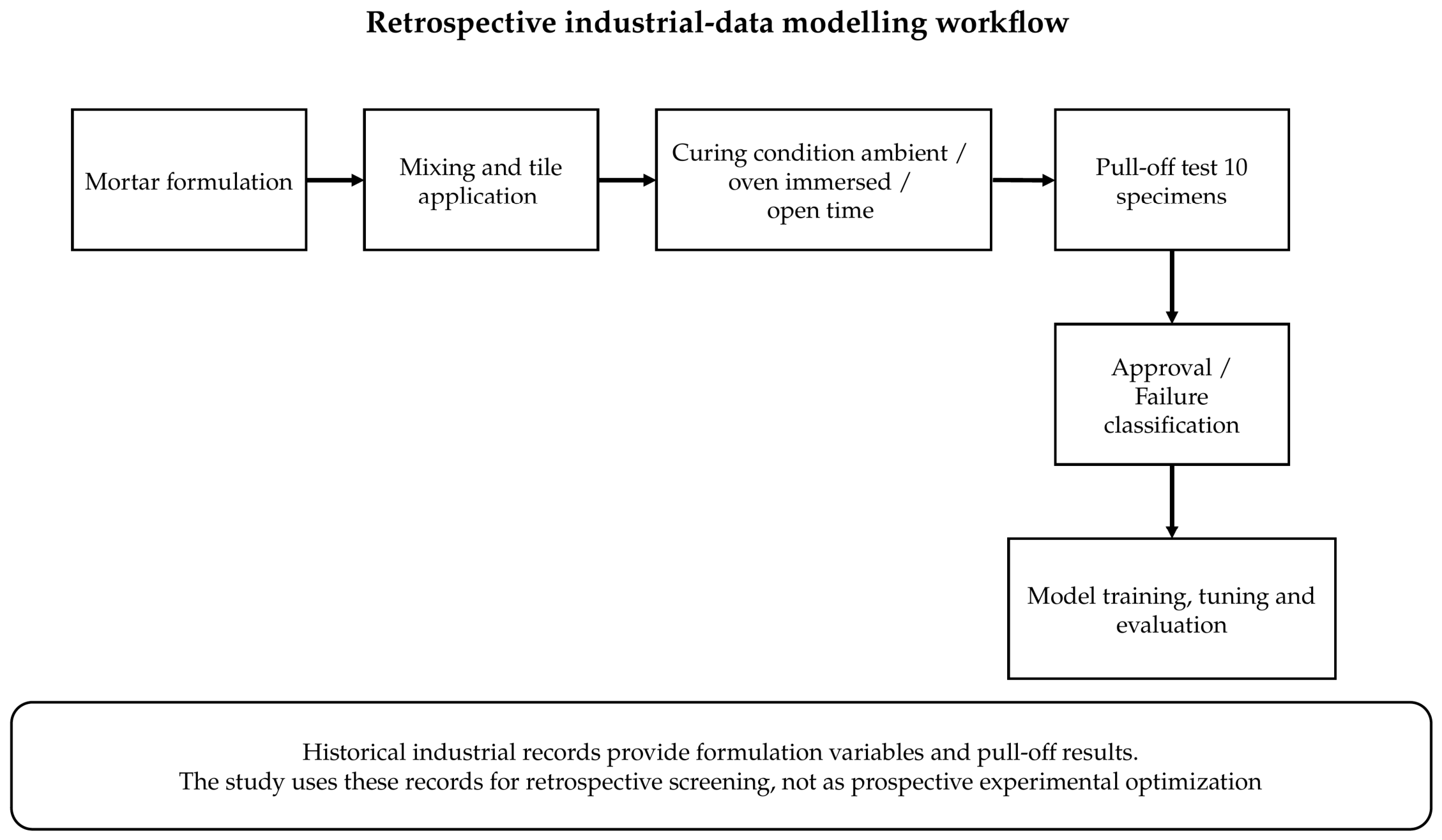
The overall experimental and retrospective modelling workflow is summarized in Figure 1.

A tile adhesive mortar is composed primarily of the following raw materials: cement, fine aggregates, chemical additives, and water. The quantities of each component depend on the quality of the raw materials and on the desired properties and cost of the final product [2,3,16].

The most commonly used cement in tile adhesive mortars is Portland cement, which plays a fundamental role in the formulation of these materials, since, when mixed with water, it reacts and transforms into a rigid and resistant material. It is, therefore, the main component responsible for the mechanical strength of the mortar and for binding all elements of the mixture together, ensuring the adhesive properties that allow the ceramic tiles to bond to the substrate. The main cement properties that can influence the performance of tile adhesive mortars are: type of cement, chemical composition, fineness, mechanical strength at different ages, and setting time [16,17].

Fine aggregates (ground sand and limestone) provide structural reinforcement to tile adhesive mortars, influencing their mechanical strength, adhesion, and especially the workability and consistency of the material after mixing with water. The particle size distribution of the sand—that is, its granulometry—is a key aspect for obtaining a mortar with ideal workability and adhesive properties. It is important that the grains vary in size, as this helps with particle packing, void filling, and achieving the ideal water content for the mortar, which in turn impacts its mechanical strength. Typically, the aggregates used in tile adhesive mortars have grains smaller than 0.8 mm [6,18].

Cellulose ether is an essential additive for tile adhesive mortars and has a significant influence on their properties in the fresh state—that is, when the mortar is still soft and workable, right after being mixed with water. It provides viscosity to the mortar, directly influencing its workability and consistency, and imparts a cohesive and adhesive characteristic to the material. This additive also helps retain water in the system, preventing it from migrating into the substrate or evaporating into the air. It improves performance in the open time test, increases the correction time during tile installation, and allows for proper cement hydration. The main properties of cellulose ether are: viscosity, degree of modification, and the chemical structure of the molecule used [6].

Redispersible polymers are added to tile adhesive mortars to improve their performance under more demanding conditions. They enable the formation of a strong chemical bond between the mortar and the ceramic covering, and also impart flexibility to the mixture—an essential characteristic for products intended for outdoor environments (AC-II and AC-III), where temperature fluctuations can cause stress between the mortar and the substrate. The flexibility provided by the polymers helps absorb these stresses and prevents the formation of cracks and fissures in the ceramic coverings, increasing the durability of the system. The main properties of redispersible polymers are: type and content of active material, PVOH (polyvinyl alcohol) content, additive content, and Tg (glass transition temperature), which indicates the polymer’s flexibility [2,6].

Accelerators are additives used in tile adhesive mortars with the purpose of speeding up the curing and hydration of Portland cement, allowing it to gain strength more quickly. In addition, they also contribute to increasing the open time, reducing permeability, and improving the strength of the mortar under heat curing conditions [19].

Water is also an essential raw material in mortars. According to the mortar formulation, there is an ideal water content—typically indicated by the manufacturer on the product packaging—that ensures proper consistency for application and guarantees final performance. Using more or less water than the ideal amount can negatively impact the properties of the mortar; therefore, determining the ideal water content is a crucial step in the development of tile adhesive mortars [17].

2.2. Presentation of the Database and Methods Used

The database used in this study was obtained from the historical records of tile adhesive mortar development tests conducted at a European multinational company in the construction materials sector. A specific subset of this historical data was selected based on the company’s interests and challenges, focusing on experimental results obtained between 2021 and the first quarter of 2023 for AC-II and AC-III mortars. Only data for these two mortar types were used because their performance is evaluated under the same conditions, with the only difference being the minimum tensile adhesion strength values required for approval in each curing condition, according to the standard. Additionally, by including both mortar types, it was possible to increase the number of observations and the variability in the proportions of raw materials used, since AC-III mortars typically require a higher amount of cement and additives to meet the superior performance demanded by the standard.

Compiling the database for this study was a challenging and labor-intensive step, as the data were scattered across various spreadsheets and folders on the company’s internal network. The data were compiled and organized using Microsoft Excel for Microsoft 365 and Power Query (Microsoft Corporation, Redmond, WA, USA) to automate the data collection process, resulting in an initial database containing 6690 observations and 75 variables. Each observation represents an individual pull-off value, meaning there are 10 different tensile adhesion strength values for each formulation and 669 total test sets.

Next, data cleaning was performed to exclude variables that were irrelevant to the study, showed little variability, had too many missing values, or whose values were deemed unreliable. Observations with missing values were also excluded during this step. After cleaning, the database contained 6031 observations and 38 variables, of which 8 were response variables (Resp.) and 30 were predictor variables (Pred.).

Table 2. Variables of the final database used for model training.

Subset	Function in Mortar	Variable Name	Type	Use
Ambient Curing	Strength (MPa)	Res_Ambiente	Num	Resp.
	Approval (Yes/No)	Res_Ambiente_Log	Cat	Resp.
Oven Curing	Strength (MPa)	Res_Estufa	Num	Resp.
	Approval (Yes/No)	Res_Estufa_Log	Cat	Resp.
Immersed Curing	Strength (MPa)	Res_Submersa	Num	Resp.
	Approval (Yes/No)	Res_Submersa_Log	Cat	Resp.
Open Time	Strength (MPa)	Res_Tempo_Aberto	Num	Resp.
	Approval (Yes/No)	Res_Tempo_Aberto_Log	Cat	Resp.
Mortar Type	Type AC-II or AC-III	Tipo_Argamassa	Cat	Pred.
Sand (10 vars)	Formulation content	Teor_Areia	Num	Pred.
	Max. Particle Size	Max_20, Max_28, Max_48, Max_100, Max_200, Max_Prato	Num	Pred.
	Min. Particle Size	Min_48, Min_100, Min_200	Num	Pred.
Cement (8 vars)	Formulation content	Teor_Cimento	Num	Pred.
	Chemical Composition	Perda_Fogo	Num	Pred.
	Fineness	Blaine, Ret_325	Num	Pred.
	Reactivity	Inicio_Pega	Num	Pred.
	Mechanical Strength	R3, R7, R28	Num	Pred.
Ether (4 vars)	Formulation content	Teor_Eter	Num	Pred.
	Chemical Composition	Eter_Tipo, Eter_Modific	Cat	Pred.
	Viscosity	Eter_Visc	Num	Pred.
Polymer (5 vars)	Formulation content	Teor_Polimero	Num	Pred.
	Chemical Composition	Pol_PVOH, Pol_Adic, Pol_Ativo	Num	Pred.
	Tg, Flexibility	Pol_Tg	Num	Pred.
Accelerator	Formulation content	Teor_Acelerador	Num	Pred.
Water Content	Formulation content	Teor_Agua	Num	Pred.

presents these variables, their respective functions in the mortar, and whether they are numerical (Num) or categorical (Cat) variables.

Data preprocessing followed a conservative approach because the database originated from routine industrial records rather than from a single planned experiment. Variables were removed when they were irrelevant to the modelling objective, had insufficient variability, contained excessive missingness, or were considered unreliable according to the internal consistency of the records. Observations with missing values in variables retained for modelling were excluded. No imputation was performed, in order to avoid artificially creating formulation–performance relationships not present in the original records. Outlier treatment was performed through domain-based inspection of physically implausible values and consistency checks against the expected range of the raw material and performance variables. The final dataset, therefore, prioritizes reliability and interpretability over maximizing the number of retained observations.

Initially, an exploratory and descriptive analysis of the data was performed using the R programming language (version 4.2.3) within the RStudio environment (version 2023.03.1-446). The modelling strategy had two complementary purposes. Logistic Regression models trained in R were used primarily for inferential analysis, because their coefficients allow the direction and approximate magnitude of the influence of formulation variables to be examined. The Azure Machine Learning Studio (classic) environment (Microsoft Corporation, Redmond, WA, USA; web-based platform, no user-visible version number available) was used primarily for predictive benchmarking among classification algorithms under a stratified training-testing split. Consequently, the R and Azure outputs should not be interpreted as strictly equivalent predictive experiments, but as complementary modelling exercises: R for interpretability and Azure for out-of-sample predictive comparison.

The Machine Learning models used in this study are summarized in

Table 3. Machine Learning models used.

No.	Model	Environment
1	Logistic Regression—Stepwise Both	R
2	Logistic Regression—Simplified	R
3	Logistic Regression	Azure
4	Random Forest	Azure
5	Boosted Decision Tree	Azure
6	Support Vector Machine	Azure

.

For all models, the response variables used were approval (considered the event, 1) or disapproval (non-event, 0) in relation to the standard. This classification was performed for each observation by comparing the tensile adhesion strength to the minimum value required by the standard for each curing condition and mortar type, according to the standard thresholds described in Section 2.1. Each observation was classified individually rather than classifying the formulation as a whole (using the average of the 10 observations and applying the standard’s calculation), as this approach allows the model to be trained with a larger dataset and incorporates the inherent variability of the test results—variations that would be reduced if only the average were used.

Because each formulation generated multiple pull-off observations, the models were trained at the specimen-observation level rather than at the formulation-average level. This choice preserved the empirical variability observed in the adhesion test and increased the number of learning instances. However, it also means that the results should be interpreted as retrospective specimen-level classification within historical formulation ranges, not as definitive prospective validation of new formulations. This limitation is explicitly considered in the interpretation of the results and in the conclusions.

Four different classification algorithms were selected with the aim of comparing their performance. Logistic regression is a statistical method that estimates the probability of an event occurring by fitting the data to a logistic function. The Random Forest algorithm is based on decision trees and combines the outputs of multiple trees, each trained on a random subset of the data, to produce the final prediction. It is more robust, accurate, and less prone to overfitting than the use of a single tree. The Boosted Decision Tree algorithm is also based on combining multiple decision trees to obtain the final prediction. However, in this case, performance is enhanced by successively creating trees with the goal of correcting the errors made by the previous one. The Support Vector Machine algorithm seeks to find the best line or hyperplane to separate two groups. This hyperplane is selected so as to maximize the distance between the closest points of each class, known as support vectors. The resulting hyperplane is then used to classify new data into one of the two categories [10,20].

The logistic regression models trained in R were obtained as follows:

• Stepwise Both: obtained through the stepwise procedure in the “both” direction, which selects statistically significant predictor variables using an algorithm that allows for both the inclusion and exclusion of variables at each iteration, depending on their contribution to the model [21]. In this study, significance was assessed using the statistical parameter p-value at the 5% level.
• Simplified: a model that uses only a subset of selected variables, with the goal of reducing multicollinearity among predictors and thus better understanding the influence of each variable on the probability of approval. Variable selection was based on the correlation matrix; when a variable pair presented a high correlation value (>0.70), a more in-depth theoretical analysis was performed, and in some cases, only one of the variables was retained for model construction. An initial model was created using all selected variables, and those with coefficients presenting p-values greater than 5% (i.e., not statistically significant) were excluded. A new model was then built, seeking to retain only variables significant at the 5% level.

In the Azure environment, the models were obtained as follows:

• Splitting the dataset into training and testing sets: 70% of the observations were used for training and 30% for testing. The split was performed in a stratified manner based on the response variable, in order to maintain the same proportion of approvals and disapprovals in both the training and testing sets.
• Training the Azure models using the training set and selecting hyperparameters with the Tune Model Hyperparameters function. The tuning procedure followed the hyperparameter-search options available in Azure Machine Learning Studio (classic). Accuracy was used operationally by the platform during tuning; however, final model interpretation was based on multiple metrics, including sensitivity, specificity, precision, balanced accuracy, F1-score and AUC, because class imbalance made accuracy alone potentially misleading.
• Evaluating the models on the testing set.

The performance of classification models is usually evaluated using a confusion matrix (

Table 4. Confusion matrix.

	Prediction: Positive (PP)	Prediction: Negative (NP)
Actual Positive (P)	True Positive (TP)	False Negative (FN)
Actual Negative (N)	False Positive (FP)	True Negative (TN)

), which shows the relationship between the model’s predictions and the actual classes present in the dataset, allowing for understanding how many and what types of errors the model is making [20,22].

Based on the data in the confusion matrix, several metrics can be calculated to practically evaluate and compare the performance of different models. The metrics used in this study are presented and explained in

Table 5. Metrics used to compare model performance.

Metric	Calculation	Explanation
Accuracy	(TP + TN)/(P + N)	Overall model efficiency; proportion of correct predictions over the total number of observations.
Sensitivity (S)	TP/(TP + FN)	Proportion of correctly predicted positive cases out of all actual positive observations.
Specificity (E)	TN/(TN + FP)	Proportion of correctly predicted negative cases out of all actual negative observations.
Precision	TP/(TP + FP)	Proportion of correct positive predictions over the total number of positive predictions made by the model.
Balanced Accuracy	(S + E)/2	Arithmetic mean of Sensitivity and Specificity; useful when there is imbalance between the number of positive and negative cases.
F1-Score	2 × (Precision × S)/(Precision + S)	Combines Precision and Sensitivity into a single metric; useful when there is class imbalance.
AUC (ROC)	Area under the S × (1 − E) curve	Summarizes the overall quality of the model, independent of the decision threshold.

Note: TP = true positive; TN = true negative; FP = false positive; FN = false negative; P = actual positive cases; N = actual negative cases; S = sensitivity; E = specificity.

[22].

In the present application, predicting non-compliant formulations is particularly relevant for product quality and risk reduction. Therefore, although accuracy is reported for comparability with common machine-learning practice, special attention is given to specificity, balanced accuracy and false-positive risk, especially in curing conditions where the number of failed observations is small.

3. Results and Discussion

This section is organized as follows: (1) exploratory and descriptive analysis of the results, presenting the main descriptive statistics for the variables and the correlation matrix; (2) presentation of the six models obtained for each curing condition (ambient, oven, immersed, and open time), with conclusions drawn from the models trained in R and comparison of the predictive capabilities of all models; and (3) comparison of the simplified logistic regression models obtained in R for each curing condition, with the coefficients obtained for the predictor variables and discussion of the influence of each variable on mortar approval.

Due to the maximum page limit imposed for this study, the coefficients and statistical significance of the variables in the logistic regression models trained in R using the Stepwise Both procedure are presented only for the ambient curing condition. This is sufficient to demonstrate the main conclusions obtained, as similar conclusions were also reached for the other curing conditions.

3.1. Exploratory and Descriptive Data Analysis

Table 6. Descriptive statistics of the numerical variables in the final dataset.

Parameter	Unit	Min	Q1	Median	Mean	Q3	Max	Std. Dev.	IQR
Res_Ambiente	MPa	0.00	1.12	1.40	1.41	1.68	3.31	0.43	0.56
Res_Estufa	MPa	0.00	0.34	0.51	0.59	0.78	2.66	0.35	0.44
Res_Submersa	MPa	0.00	0.56	0.74	0.75	0.93	1.97	0.27	0.37
Res_Tempo_Aberto	MPa	0.00	0.68	0.96	0.96	1.23	2.49	0.40	0.55
Teor_Cimento	10−3	52.0	250.0	280.0	290.4	340.0	480.0	63.2	90.0
Teor_Areia	10−3	100.0	633.7	705.0	666.8	731.3	778.3	102.1	97.6
Teor_Eter	10−3	1.4	1.8	2.1	2.3	2.8	3.6	0.6	1.0
Teor_Polimero	10−3	0.0	7.0	9.0	8.9	10.0	17.0	2.4	3.0
Teor_Acelerador	10−3	0.0	0.0	2.0	3.4	7.0	14.5	4.1	7.0
Teor_Agua	%	19.0	21.5	23.0	23.8	26.0	32.5	2.8	4.5
Eter_Visc	mPa·s	10,000	20,000	25,000	29,376	40,000	70,000	14,338	20,000
Pol_PVOH	%	0.0	4.6	5.9	6.5	8.1	9.8	2.1	3.5
Pol_Adic	%	0.0	0.0	0.0	6.0	7.3	27.3	8.5	7.3
Pol_Ativo	%	0.0	48.2	58.6	59.9	72.5	76.0	14.5	24.3
Pol_Tg	°C	0.0	19.2	21.5	24.9	37.4	43.9	9.1	18.2
Perda_Fogo	%	0.6	4.0	6.0	6.1	7.7	10.5	2.5	3.7
Blaine	cm2/g	3604	4202	4670	4617	4904	5683	509	702
Ret_325	%	0.5	1.4	3.0	4.3	6.8	11.6	3.4	5.4
Inicio_Pega	min	120.0	148.0	170.0	180.4	213.0	277.0	43.0	65.0
R3	MPa	18.5	24.6	31.5	29.5	34.8	37.0	5.7	10.2
R7	MPa	23.6	29.7	37.1	35.5	40.4	43.1	5.7	10.7
R28	MPa	32.2	36.3	44.6	43.4	47.5	54.5	6.9	11.2
Max_20	%	0.0	1.0	2.0	2.3	3.0	8.0	1.9	2.0
Max_28	%	0.7	5.0	6.0	8.3	10.0	50.0	8.1	5.0
Max_48	%	12.0	45.0	55.0	51.1	62.3	85.0	16.9	17.3
Max_100	%	19.3	40.0	55.0	52.9	60.0	95.0	18.2	20.0
Max_200	%	1.0	10.0	15.0	17.1	25.0	40.0	9.6	15.0
Max_Prato	%	0.1	2.0	3.0	4.1	5.0	10.0	2.4	3.0
Min_48	%	0.0	20.0	30.0	28.0	35.0	65.0	17.5	15.0
Min_100	%	10.0	20.0	25.0	31.0	30.0	80.0	17.2	10.0
Min_200	%	0.0	0.0	4.0	3.9	5.0	20.0	4.1	5.0

presents descriptive statistical measures for the numerical variables: unit of measurement, minimum, maximum, and mean values, median, first and third quartiles, standard deviation, and interquartile range (third quartile value−first quartile value).

Table 7. Descriptive statistics of the categorical variables.

Categorical Variable	Category	Frequency	%
Res_Ambiente_Log	Approved	5763	96%
	Not Approved	268	4%
Res_Estufa_Log	Approved	2026	34%
	Not Approved	4005	66%
Res_Submersa_Log	Approved	3680	61%
	Not Approved	2351	39%
Res_Tempo_Aberto_Log	Approved	5317	88%
	Not Approved	714	12%
Tipo_Argamassa	AC II	3719	62%
	AC III	2312	38%
Eter_Tipo	MHEC	3219	53%
	MHPC	2812	47%
Eter_Modific	Modified	4403	73%
	Non-modified	1628	27%

presents the observed frequencies for the 7 categorical variables in the dataset. The Oven Curing condition (Res_Estufa_Log) showed approval in only 34% of the observations, followed by Immersed Curing (Res_Submersa_Log) with 61% approval, Open Time (Res_Tempo_Aberto_Log) with 88%, and Ambient Curing with 96%. These values are consistent with experimental observations, since Ambient and Open Time curing conditions rarely present approval issues for AC-II and AC-III mortars. However, as the data are imbalanced, this may pose challenges in developing models capable of effectively predicting disapproval in these curing conditions, given that there are few observations related to disapproval in the dataset.

The variable Tipo_Argamassa has only two categories, with the majority of observations (62%) corresponding to type AC-II. The variables related to cellulose ether also have only two categories: Eter_Tipo shows a more balanced distribution, with 53% of observations in the MHEC category and 47% in MHPC, while for Eter_Modific, 73% of observations are of the Modified type and only 27% are Non-modified.

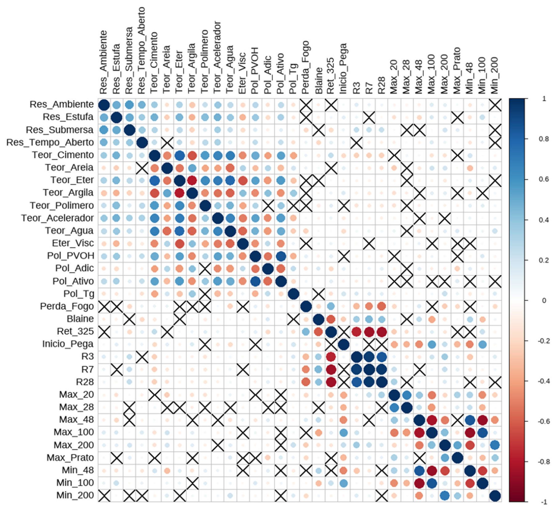
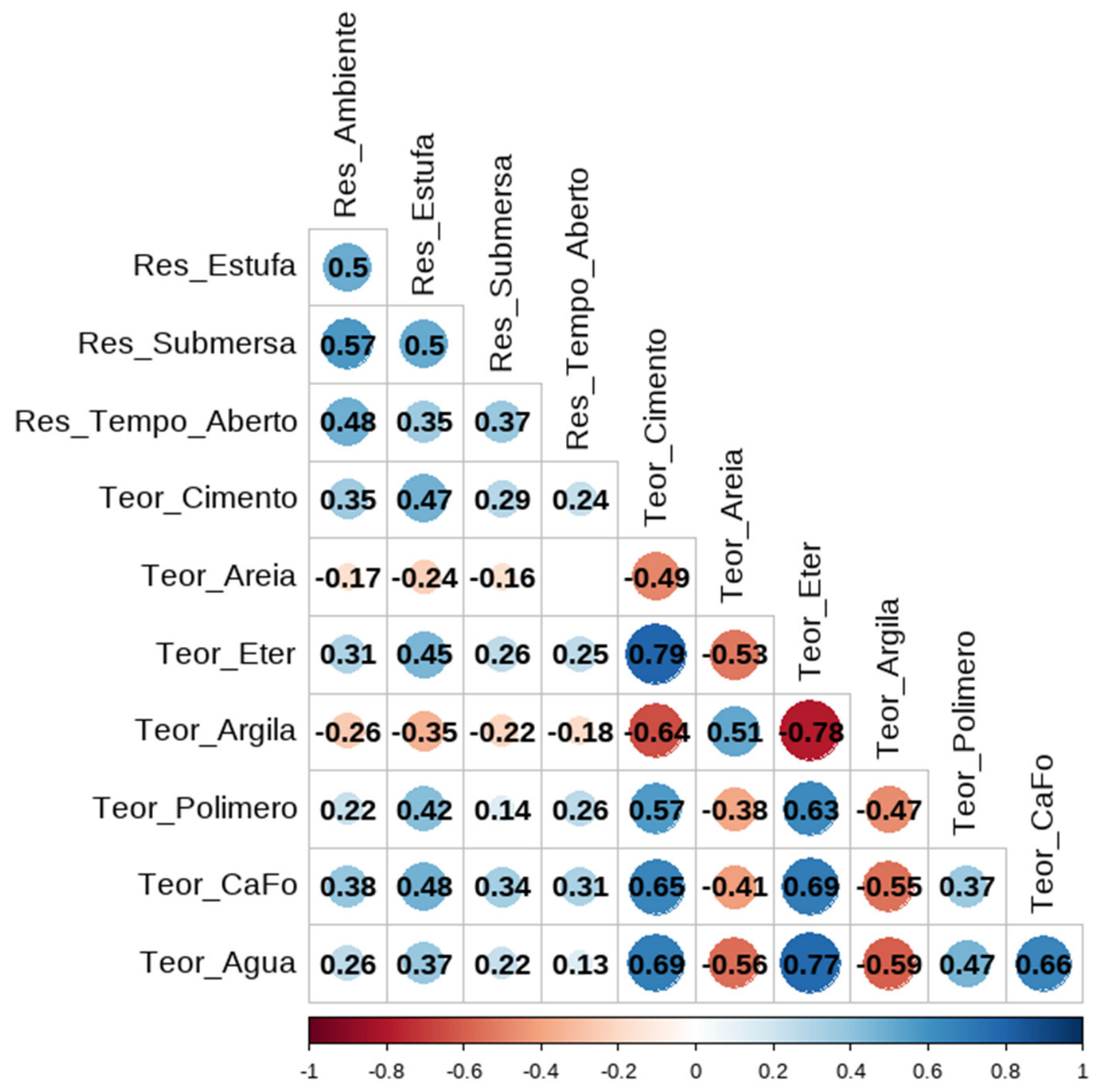
Figure 2 presents the correlation matrix for all numerical variables. Black X symbols indicate pairs without statistically significant correlation at the 5% significance level. The complete matrix is useful as an exploratory diagnostic because it shows both formulation–performance associations and strong correlations among predictors. Figure 3 provides a focused view of the relationships between curing-performance variables and main formulation contents, which is easier to interpret and is therefore used as the main visual basis for discussing the formulation variables.

Another important point is that there is a high correlation among the predictor variables, with some of them even showing stronger correlations with each other than with the response variables. This can lead to multicollinearity issues in the models, which may impair their predictive performance and make it more difficult to interpret the coefficients obtained for the predictor variables. Some of these correlations are theoretically justified—for example, the correlations among the contents of raw materials and within each group of raw material properties (e.g., the group of polymer properties, cement properties, and sand granulometry). Other correlations, however, appear to be coincidental, such as those between the variable Inicio_Pega (a property of cement) and variables related to sand granulometry.

The analysis of the correlation matrix also supported the selection of variables for the construction of the simplified model. The variables Min_48, Min_100, and Min_200, which refer to the minimum granulometry of sand, show high correlations (>0.70) with the variables Max_48, Max_100, and Max_200, and therefore will not be used. Moreover, it is theoretically coherent to use only the maximum sand granulometry values. Regarding the cement properties, it was observed that the variables R3, R7, and R28, which refer to the cement’s strength at different ages (3, 7, and 28 days, respectively), present high correlations (>0.80) among themselves. In this case, only the variable R3 was retained for the simplified model, using as theoretical reference the decision made by Monaco and Carrà [16], who used only the compressive strength at 2 days as an indicator of cement quality. At the end of this process, the selected variables for the simplified model totaled 24, namely: Teor_Cimento, Teor_Areia, Teor_Eter, Teor_Polimero, Teor_Acelerador, Teor_Agua, Eter_Visc, Eter_Tipo_MHPC, Eter_Modific_NON_MODIFIED, Pol_PVOH, Pol_Adic, Pol_Ativo, Pol_Tg, Perda_Fogo, Blaine, Ret_325, Inicio_Pega, R3, Max_28, Max_48, Max_100, Max_200, Max_Prato, and Tipo_Argamassa_AC_III.

3.2. Models for Ambient Curing

Table 8. Comparison of logistic regression models for ambient curing.

Predictor Variable	Stepwise Both: Coef. (SE)	VIF	Simplified: Coef. (SE)	VIF
Intercept	−7.630 ** (3.222)	—	−7.066 *** (1.683)	—
Teor_Cimento	0.018 *** (0.002)	5.66	0.015 *** (0.002)	4.59
Teor_Areia	0.004 *** (0.001)	2.56	0.003 *** (0.001)	1.83
Teor_Eter	1.321 *** (0.472)	15.43	—	—
Teor_Polimero	0.208 *** (0.047)	2.83	0.262 *** (0.043)	2.27
Teor_Acelerador	0.192 *** (0.027)	2.79	0.142 *** (0.025)	2.50
Tipo_Argamassa_AC_III	−4.955 *** (0.549)	16.17	−4.202 *** (0.301)	4.96
Eter_Visc	0.00002 ** (0.00001)	2.99	—	—
Eter_Tipo_MHPC	0.422 ** (0.190)	2.01	0.646 *** (0.148)	1.24
Pol_Adic	0.045 *** (0.014)	2.52	—	—
Pol_Tg	−0.025 ** (0.010)	1.99	—	—
Perda_Fogo	0.072 ** (0.029)	1.30	—	—
Blaine	−0.001 *** (0.0003)	6.38	−0.001 *** (0.0002)	2.24
Ret_325	0.231 *** (0.075)	11.35	—	—
R3	−0.235 ** (0.100)	80.25	0.137 *** (0.019)	2.79
R7	0.869 *** (0.218)	309.12	—	—
R28	−0.383 *** (0.113)	123.97	—	—
Max_20	0.342 *** (0.102)	9.24	—	—
Max_28	−0.040 ** (0.017)	3.50	—	—
Max_48	0.036 *** (0.009)	5.25	—	—
Max_100	0.021 ** (0.008)	6.19	—	—
Max_200	0.071 *** (0.025)	10.66	0.032 *** (0.012)	2.44
Max_Prato	−0.356 *** (0.067)	5.75	—	—
Min_48	−0.068 *** (0.014)	15.84	—	—
Min_100	−0.074 *** (0.013)	15.26	—	—
Min_200	−0.124 *** (0.029)	2.84	—	—

Significance levels: ** p < 0.05; *** p < 0.01.

presents the two logistic regression models obtained in R for predicting formulation approval under ambient curing: stepwise both and simplified. The coefficients for each variable are shown, along with their respective statistical significance (represented by the number of asterisks next to the coefficient value), the standard error of each coefficient (shown in parentheses), and the results of the Variance Inflation Factor (VIF) test for each coefficient, which helps identify whether there are multicollinearity issues among the predictor variables.

The models obtained through the two different methods differed in the number of predictor variables and in the values of their coefficients. The model generated by the stepwise both procedure includes a larger number of explanatory variables (21) and exhibits quite pronounced multicollinearity issues. Multicollinearity is assessed through the VIF values: the higher the VIF, the greater the presence of multicollinearity for that variable. Typically, the interpretation is as follows: low collinearity for VIF < 5, moderate for VIF between 5 and 10, and high for VIF > 10. The variables R7 and R28 showed VIF > 100, indicating severe multicollinearity—unsurprising, given that their correlations with R3 exceed 0.95. Other variables that also presented VIF > 10 include: Teor_Eter, Tipo_Argamassa_AC_III, Ret_325, R3, Max_200, Min_48, and Min_100.

The simplified model, on the other hand, contains a smaller number of predictor variables (13) and did not show significant multicollinearity issues, indicating that the variable selection was effective. In this model, the variables with VIF > 5—and therefore moderate collinearity—were Max_48 and Max_100, which refer to sand granulometry. Although these variables are highly correlated with each other (−0.83), both were retained in the simplified model since they are always available and important for characterizing the properties of tile adhesive mortar.

Some predictor variables are present in both models, while others appear in only one. Most of the variables that appear in both models showed similar coefficient values, with the same order of magnitude and the same sign. However, the variable R3 displayed opposite signs in each model—negative in the stepwise model and positive in the simplified one—which occurred due to the high multicollinearity present in the stepwise both model between the variables R3, R7, and R28.

It can therefore be concluded that the simplified model offers better interpretability and more reliable insight into the impact of each predictor variable on approval under a given curing condition, as the predictor variables in this model exhibit lower intercorrelation. A good example of this is the set of variables R3, R7, and R28: in the Stepwise Both model, they showed conflicting coefficient signs—R3 (−0.235) and R28 (−0.383) were negative, while R7 (0.869) was positive. When analyzing the coefficients for R3 or R28 in isolation, they do not make theoretical sense, as it is expected that a mortar made with stronger cement would have a higher probability of approval under ambient curing. When all three variables are considered together, one may offset the other, and ultimately, using stronger cement may result in higher approval rates. However, this cannot be concluded quickly by just looking at the coefficient signs. In contrast, the simplified model includes only the R3 variable, with a coefficient of 0.137, clearly indicating that stronger cement increases the likelihood of approval in ambient curing.

Table 9. Main performance metrics of the models for ambient curing.

Metric	LR (R) Stepwise	LR (R) Simplified	LR (Azure)	Random Forest	Boosted DT	SVM
Cutoff	0.650	0.650	0.550	0.450	0.500	0.500
Accuracy	0.962	0.960	0.962	0.965	0.965	0.962
Sensitivity	0.999	1.000	1.000	0.999	0.999	1.000
Specificity	0.153	0.104	0.150	0.238	0.238	0.150
Precision	0.962	0.960	0.962	0.966	0.966	0.962
Balanced Accuracy	0.576	0.552	0.575	0.618	0.618	0.575
F1-Score	0.980	0.979	0.981	0.982	0.982	0.981
AUC	0.803	0.788	0.790	0.758	0.736	0.774

reports the predictive performance metrics for the models obtained for ambient curing. Because the Logistic Regression models trained in R and the models trained in Azure were generated under different protocols, the table should be read with caution: the R models are mainly used for inference, whereas the Azure models provide the principal basis for out-of-sample predictive comparison. The cutoff point selected was the one that resulted in the highest accuracy and varied according to the algorithm used. Based on specificity and balanced accuracy, Random Forest and Boosted Decision Tree performed better than the other models, although all models were strongly affected by the very low prevalence of failures under this curing condition.

Although all models presented accuracy above 96%, their specificity was very low across the board, indicating that the models are not effective at predicting disapproval outcomes in this curing condition. This likely occurred due to the characteristics of the dataset used, which is highly imbalanced, containing only 4% of observations classified as not approved for this curing condition. From a business standpoint, this conclusion is not surprising, as after averaging the results obtained from the 10 test specimens, disapproval under ambient curing is rarely observed for AC-II and AC-III products.

The Random Forest and Boosted Decision Tree models, although they demonstrated better predictive capabilities compared to logistic regression models, cannot be used to make inferences or draw conclusions about the influence of each variable on mortar approval as easily and directly as logistic regression models. This is because their algorithms are more complex, allowing for intricate interactions between variables, and they rely on the combination of multiple decision trees, each with different weights and variables, which are ultimately aggregated to make predictions. For this reason, these models are referred to as black-box models, as it is not possible to fully understand how their predictions are made. Nonetheless, there are techniques and approaches that can increase the interpretability of such models, including Feature Importance analysis, Partial Dependence Plots (PDP), and SHAP Values, which provide insights and enable some conclusions about how the models are making decisions. Even so, these models are still not fully interpretable [9,10].

Although the simplified logistic regression model demonstrated lower predictive performance, it offers easier and more straightforward interpretation than the other models, and for this reason, it was selected to perform inference and draw conclusions regarding the influence of each variable on the approval of tile adhesive mortars under each curing condition.

The differences between the metrics obtained for the Logistic Regression model trained in Azure and the Logistic Regression models trained in R are partly explained by the different modelling purposes and validation protocols. In R, the models were fitted to support inferential interpretation of coefficients and multicollinearity diagnostics. In Azure, the dataset was split into training and testing sets in order to evaluate predictive performance on held-out observations. For this reason, the manuscript does not treat the R and Azure results as a perfectly controlled algorithmic competition, but as complementary evidence addressing interpretability and predictive screening.

This distinction is important for practical interpretation. R offers greater control over modelling assumptions, variable selection and coefficient interpretation, which is relevant for understanding the physical meaning of formulation variables. Azure, in contrast, provides a rapid graphical workflow for comparing several algorithms under a common training-testing split, but with less transparency regarding all internal tuning choices. The conclusions, therefore, emphasize broad patterns that are robust across metrics and curing conditions rather than small numerical differences between environments.

3.3. Models for Oven Curing

As with ambient curing, two logistic regression models were obtained in R—stepwise both and simplified—to predict approval under oven curing conditions. The table comparing the coefficients obtained for each model was omitted due to the page limit. However, the comparison was conducted, and the main conclusions drawn from this analysis are as follows: both models for oven curing presented a greater number of predictor variables that were statistically significant at the 5% level than those for ambient curing—23 for the stepwise both model and 20 for the simplified model. Furthermore, the stepwise model for oven curing exhibited less pronounced multicollinearity issues (VIF values < 20) than the one obtained for ambient curing. The variables with high collinearity (VIF > 10) were Max_48, Min_100, and R28; and those with moderate collinearity (5 < VIF < 10) included Teor_Eter, Tipo_Argamassa_AC_III, Ret_325, R3, and Max_20—which also presented multicollinearity issues in the ambient curing model. As with the previous curing condition, the simplified model also helped reduce the VIF of the predictor variables, with only Ret_325, Tipo_Argamassa_AC_III, and Pol_PVOH exhibiting moderate collinearity (VIF > 5).

Table 10. Main performance metrics of the models for oven curing.

Metric	LR (R) Stepwise	LR (R) Simplified	LR (Azure)	Random Forest	Boosted DT	SVM
Cutoff	0.425	0.425	0.450	0.430	0.500	0.480
Accuracy	0.715	0.706	0.731	0.816	0.822	0.727
Sensitivity	0.554	0.531	0.492	0.771	0.707	0.398
Specificity	0.797	0.794	0.853	0.839	0.880	0.893
Precision	0.580	0.566	0.628	0.708	0.749	0.654
Balanced Accuracy	0.676	0.662	0.672	0.805	0.794	0.646
F1-Score	0.567	0.548	0.552	0.739	0.728	0.495
AUC	0.754	0.745	0.762	0.890	0.890	0.751

presents the metrics used to compare the performance of the six models obtained for predicting approval under oven curing. As with ambient curing, the cutoff points were selected to maximize model accuracy and varied among the models, ranging from 0.425 to 0.5. These values were lower than those obtained for ambient curing models, which ranged from 0.45 to 0.65. Similarly, the Random Forest and Boosted Decision Tree models showed superior predictive capabilities compared to the others, with particular emphasis on the metrics: sensitivity, precision, balanced accuracy, and F1-score, which were significantly higher for these models. Furthermore, unlike what was observed for ambient curing, these two models also presented higher values for the Area Under the ROC Curve than the others.

The decision as to which of these two models is better is not straightforward, since some metrics are better for one model and others for the other. The Boosted Decision Tree model showed higher values for accuracy (+0.7%), specificity (+4.9%), and precision (+5.8%), while the Random Forest model had higher values for sensitivity (+9.1%), balanced accuracy (+1.4%), and F1-score (+1.5%). From a business perspective, achieving higher specificity is more desirable than higher sensitivity. This is because, in terms of product quality, it is less problematic to predict that a mortar would fail but it actually passes (false negative, related to sensitivity) than to predict that a mortar would pass and it actually fails (false positive, related to specificity). Therefore, based on these considerations, it is concluded that the model with the best performance for oven curing is the Boosted Decision Tree.

3.4. Models for Immersed Curing

The table comparing the two logistic regression models obtained in R (stepwise both and simplified) for immersed curing also had to be omitted due to space limitations. However, the analysis was conducted, and the main conclusions were as follows: similar to what was observed for the ambient and oven curing models, the stepwise both model for immersed curing also included a greater number of predictor variables (20) and presented multicollinearity issues among them. The variables with high collinearity (VIF > 10) were Max_48, Max_100, Min_48, and Min_100, all related to sand granulometry. The variables Ret_325, R7, Pol_PVOH, Pol_Ativo, Tipo_Argamassa_AC_III, and Teor_Cimento showed VIF > 5, indicating moderate collinearity.

The simplified model, in turn, included 19 significant variables, some of which also exhibited only moderate collinearity—namely Max_48, Max_100, Tipo_Argamassa_AC_III, Ret_325, Pol_PVOH, Pol_Ativo, and Teor_Cimento.

Table 11. Main performance metrics of the models for immersed curing.

Metric	LR (R) Stepwise	LR (R) Simplified	LR (Azure)	Random Forest	Boosted DT	SVM
Cutoff	0.590	0.580	0.520	0.430	0.310	0.590
Accuracy	0.790	0.785	0.794	0.883	0.886	0.796
Sensitivity	0.814	0.821	0.841	0.965	0.968	0.831
Specificity	0.752	0.729	0.719	0.755	0.756	0.742
Precision	0.837	0.826	0.824	0.860	0.861	0.834
Balanced Accuracy	0.783	0.775	0.780	0.860	0.862	0.786
F1-Score	0.825	0.823	0.833	0.909	0.912	0.833
AUC	0.844	0.841	0.846	0.937	0.938	0.843

presents the metrics used to compare the performance of the six models obtained for immersed curing. As with the models developed for the other two curing conditions, differences were observed in the cutoff point chosen for each algorithm, with the choice again being made to maximize model accuracy. Once more, the models with the best performance were Random Forest and Boosted Decision Tree, with consistently high metric values (>0.75) and a particular emphasis on accuracy and sensitivity, which were significantly better for these two models (by more than 13%) compared to the other four.

For immersed curing, however, there is no doubt as to which model had the best predictive performance: the Boosted Decision Tree algorithm outperformed Random Forest across all metrics, even though the difference was small. Nevertheless, it is important to note that the Boosted Decision Tree model took the longest to train. Thus, depending on the size of the dataset, it may be more practical to use the Random Forest algorithm, which delivered nearly equivalent performance but was trained more quickly.

Another noteworthy point is that for immersed curing, even the simpler algorithms—logistic regression and Support Vector Machine—also showed strong predictive performance, being more efficient for this curing condition than for the others. This indicates that the dataset used has a significant impact on the quality of the model obtained.

3.5. Models for Open Time

The table comparing the logistic regression models obtained in R for predicting approval under open time conditions was also omitted, but the conclusions drawn were as follows: the Stepwise Both model again included a greater number of predictor variables than the simplified model (21 and 16, respectively) and exhibited multicollinearity issues. The variables that showed high collinearity (VIF > 10) in the Stepwise Both model were Min_100, Max_100, Min_48, Max_48, Teor_Eter, and Tipo_Argamassa_AC_III. The simplified model addressed this issue, including only predictor variables with VIF < 10 and therefore only moderate collinearity, specifically Teor_Eter and Tipo_Argamassa_AC_III.

Table 12. Main performance metrics of the models for open time.

Metric	LR (R) Stepwise	LR (R) Simplified	LR (Azure)	Random Forest	Boosted DT	SVM
Cutoff	0.600	0.600	0.490	0.510	0.520	0.500
Accuracy	0.888	0.887	0.886	0.898	0.904	0.886
Sensitivity	0.991	0.989	0.999	0.974	0.966	0.999
Specificity	0.120	0.130	0.037	0.332	0.439	0.042
Precision	0.894	0.894	0.886	0.916	0.928	0.886
Balanced Accuracy	0.556	0.559	0.518	0.653	0.703	0.521
F1-Score	0.940	0.939	0.939	0.944	0.947	0.939
AUC	0.763	0.752	0.743	0.836	0.844	0.720

presents the metrics used to compare the predictive performance of the six models obtained for open time. The cutoff point was again selected to maximize accuracy and differed for each model. The conclusions for this curing condition are very similar to those obtained for the previous ones: the models that performed best were Random Forest and Boosted Decision Tree, with higher values than the other four models for all metrics, except sensitivity, which was lower. For open time, the Boosted Decision Tree algorithm showed significantly better performance than Random Forest for the specificity and balanced accuracy metrics, indicating that it was more effective at predicting failures under this curing condition. On the other hand, this improvement in predicting disapprovals resulted in lower performance for predicting approvals, as indicated by the lower sensitivity of this model compared to the others. Since, from a business perspective, a more balanced model is preferred, the conclusion is that Boosted Decision Tree is more suitable for predicting performance under open time conditions.

3.6. Comparison of Simplified Logistic Regression Models Obtained in R

Table 13. Comparison of simplified models across all curing conditions.

Variable	Ambient	Oven	Immersed	Open Time
Intercept	−7.066 ***	−13.088 ***	−19.461 ***	−8.904 ***
Teor_Cimento	0.015 ***	0.011 ***	0.017 ***	—
Teor_Areia	0.003 ***	−0.001 ***	0.005 ***	—
Teor_Eter	—	—	—	0.556 **
Teor_Polimero	0.262 ***	0.144 ***	—	0.184 ***
Teor_Acelerador	0.142 ***	0.173 ***	0.168 ***	0.208 ***
Teor_Agua	—	−0.093 ***	−0.049 **	—
Tipo_Argamassa_AC_III	−4.202 ***	−3.033 ***	−4.415 ***	−0.735 ***
Eter_Tipo_MHPC	0.646 ***	0.583 ***	0.544 ***	—
Eter_Visc	—	−0.00003 ***	0.00003 ***	—
Eter_Modific_NON_MODIFIED	—	—	0.683 ***	—
Pol_PVOH	—	0.303 ***	0.158 ***	—
Pol_Adic	—	0.044 ***	0.019 ***	—
Pol_Ativo	—	−0.019 ***	−0.032 ***	0.012 ***
Pol_Tg	−0.025 **	0.021 ***	0.015 ***	−0.023 ***
Perda_Fogo	0.072 **	−0.086 ***	−0.157 ***	—
Blaine	−0.001 ***	0.001 ***	0.001 ***	−0.001 ***
Ret_325	—	0.201 ***	0.098 ***	—
Inicio_Pega	—	0.003 ***	0.015 ***	0.007 ***
R3	0.137 ***	0.121 ***	0.081 ***	0.052 ***
Max_48	0.036 ***	0.072 ***	0.047 ***	—
Max_28	—	0.030 ***	0.048 ***	0.026 ***
Max_100	0.021 **	0.025 ***	0.066 ***	0.031 ***
Max_200	0.032 ***	0.014 ***	0.036 ***	0.028 ***
Max_Prato	—	—	—	0.157 ***

Significance levels: ** p < 0.05; *** p < 0.01.

presents a comparison between the simplified models obtained for each curing condition. It is notable that the intercept showed negative values and was statistically significant at the 1% level for all curing types. Additionally, the predictor variables were not the same across all models. This occurred because, although all simplified models were initially built using the same set of variables, some of them were excluded later as they were not statistically significant at the 5% level.

The variables present in all curing conditions were Teor_Acelerador, Tipo_Argamassa_AC_III, Pol_Tg, Blaine, R3, Max_100, and Max_200. Most of these variables had coefficients with the same sign across all curing conditions, while Pol_Tg and Blaine had negative coefficients for ambient curing and open time, and positive ones for oven and immersed curing.

The variable Teor_Acelerador had positive coefficients with similar magnitudes for all curing types, indicating that the higher its content in the formulation, the greater the likelihood of mortar approval across all curing conditions.

The variable Tipo_Argamassa_AC_III had negative coefficients for all curing conditions, with similar magnitudes for ambient, oven, and immersed curing, and a smaller magnitude for open time. This suggests that being an AC-III mortar reduces the chances of approval more for the first three curing conditions than for open time. This makes sense, since the minimum requirement for approval in open time is the same (0.5 MPa) for both AC-II and AC-III mortars, whereas in the other curing conditions, there is a difference (0.5 MPa for AC-II and 1.0 MPa for AC-III), making it more difficult for an AC-III mortar to be approved compared to an AC-II.

The variable R3 also showed positive coefficients across all curing conditions, indicating that the higher the cement’s compressive strength at 3 days, the greater the probability of mortar approval. However, the coefficient magnitudes varied by curing condition, decreasing in the following order: ambient, oven, immersed, and open time—suggesting that stronger cement has a greater impact on approval probability in ambient and oven curing than in immersed curing and open time.

The variable Teor_Cimento proved important for predicting approval in ambient, oven, and immersed curing, but was not significant at the 5% level for predicting approval under open time when other variables were included in the model. Its influence is as follows: the higher the cement content in the formulation, the greater the likelihood of mortar approval in ambient, oven, and immersed curing.

The variable Teor_Eter remained only in the final model for open time and had a positive coefficient. However, Teor_Cimento was excluded from this model due to a high correlation (0.79) between the two variables. When one of these variables is already in the model, the other becomes unnecessary for explaining the variance. However, this does not mean that mortar can be made without either ether or cement—it only implies that, due to the correlation, including both in the model is redundant for predicting approval under these conditions.

The variable Teor_Polimero was relevant for predicting approval in ambient, oven, and open time curing, but did not remain in the final model for immersed curing. The coefficient signs were positive, indicating that a higher polymer content in the formulation increases the probability of mortar approval in these curing types.

Similarly, it is possible to make inferences regarding the influence of other variables on curing outcomes; however, this was not done in this study due to space limitations.

The interpretation of Logistic Regression coefficients should nevertheless remain cautious. Coefficient signs and statistical significance indicate associations within the observed industrial dataset, not causal effects that can be generalized outside the sampled formulation ranges. Some variables also represent formulation decisions that are physically and commercially coupled; therefore, interactions among cement content, sand granulometry, cellulose ether, polymer properties and water demand may be partially captured by the predictive models but are not fully decomposed by the simplified Logistic Regression models. This is why the inferential analysis is used as formulation guidance rather than as a complete mechanistic explanation of mortar behaviour.

3.7. Comparison of the Metrics for the Best-Performing Models for Each Curing Condition

Table 14. Metrics of the best-performing models for each curing condition.

Metric	Ambient (Random Forest)	Oven (Boosted DT)	Immersed (Boosted DT)	Open Time (Boosted DT)
Cutoff	0.450	0.500	0.310	0.520
Accuracy	0.965	0.822	0.886	0.904
Sensitivity	0.999	0.707	0.968	0.966
Specificity	0.238	0.880	0.756	0.439
Precision	0.966	0.749	0.861	0.928
Balanced Accuracy	0.618	0.794	0.862	0.703
F1-Score	0.982	0.728	0.912	0.947
AUC	0.758	0.890	0.938	0.844

allows for a comparison of the predictive capabilities of the best-performing models obtained for each curing condition. All models showed good performance, with accuracy above 80% across all curing conditions. Overall, the algorithm that delivered the best performance was the Boosted Decision Tree, which was outperformed by Random Forest only in the ambient curing condition.

Overall, the model obtained for immersed curing outperformed those developed for the other curing conditions. It was possible to achieve high accuracy (87%) along with high sensitivity (97%) and specificity (76%)—a combination not observed for any of the other curing conditions. The models developed for ambient curing and open time achieved very high accuracy and sensitivity (above 90%), but lower specificity (below 45%). For oven curing, the model had lower accuracy (82%), higher specificity compared to the others (88%), and lower sensitivity (71%).

The models obtained for ambient curing and open time displayed similar behaviour: both achieved higher accuracy, sensitivity, and precision, but lower specificity. This was due to the fact that the datasets used to train these models were imbalanced, with approval rates above 85% for these two curing conditions, and therefore did not contain enough disapproval samples to train the models effectively. Balanced accuracy is a useful metric for comparing model performance when the dataset is imbalanced. Based on this metric, it is possible to conclude that the models for immersed and oven curing performed better than those for ambient curing and open time.

From an industrial standpoint, the imbalance observed for ambient curing and open time should not be ignored. It limits the ability of the models to identify rare non-compliant formulations under these two conditions. At the same time, the imbalance reflects the historical behaviour of AC-II and AC-III products in the company database, where failures under ambient curing and open time were uncommon. Consequently, the models are more useful for screening risk under oven and immersed curing than for detecting rare failures under ambient curing and open time.

3.8. Limitations and Implications for Industrial Use

This study has four main limitations. First, the models were trained using historical data from a single company, which may reflect specific raw materials, suppliers, formulation practices and laboratory procedures. Second, no independent external dataset or prospective experimental campaign with newly proposed formulations was available. Therefore, the models should not be interpreted as validated tools for unrestricted production deployment. Third, class imbalance reduced the reliability of failure prediction under ambient curing and open time. Fourth, the models are valid only within the formulation and raw-material ranges represented in the historical dataset; predictions outside these ranges should be considered unreliable until experimentally verified.

Despite these limitations, the results are relevant for industrial formulation screening. The models can help prioritize which candidate formulations deserve laboratory testing, identify curing conditions where failure risk is higher, and support interpretation of how formulation variables are associated with approval probability. The appropriate use of the models is therefore decision support, not replacement of normative testing. Future work should combine model-assisted formulation optimization with prospective laboratory validation, ideally using designed experiments or temporally separated industrial batches to assess generalization under new production conditions. Future research could also develop integrated multi-output or formulation-level models capable of jointly estimating approval across all curing conditions, since industrial approval depends on simultaneous compliance with the full set of normative requirements.

4. Conclusions

• This study evaluated whether historical industrial data can be used to train Machine Learning models to predict the approval or failure of tile adhesive mortars under the four curing conditions defined by ABNT NBR 14081/2012.
• The best predictive results were obtained with tree-based ensemble models. Boosted Decision Tree achieved the best performance in oven, immersed and open-time curing, whereas Random Forest performed best for ambient curing.
• Model performance was not uniform across curing conditions. The strongest and most balanced predictive performance was observed for immersed and oven curing. Ambient curing and open time showed high accuracy but low specificity because failures were rare in the historical dataset.
• Logistic Regression was retained for inferential interpretation because its coefficients support a clearer discussion of the direction of influence of formulation variables, even though its predictive performance was generally lower than that of the ensemble models.
• The results support the use of Machine Learning as a decision-support tool for formulation screening and quality-risk prioritization, but not as a substitute for normative testing or prospective experimental validation.
• The main limitations are the use of data from a single company, the absence of external validation, the absence of newly designed experimental formulations and the restriction of predictions to the formulation ranges observed in the historical dataset. Future studies should combine model-assisted optimization with prospective laboratory validation. Future studies could also develop integrated multi-output or formulation-level models capable of jointly estimating approval across all curing conditions, reflecting the fact that industrial approval depends on simultaneous compliance with the full set of normative requirements.