RT-DETR-Based Small-Sample Defect Detection for Solar Vacuum Glass Collector Tubes

Abstract

To address the challenges of limited samples, class imbalance, and real-time requirements in surface defect detection for solar vacuum glass collector tubes, this study proposes an improved lightweight RT-DETR-based method. Specifically, DICM is introduced into the backbone to improve multi-directional and multi-scale feature extraction, HAFB is embedded in the neck to enhance the fusion of local details and global semantics, and transfer learning is adopted to alleviate data scarcity under small-sample conditions. Experiments on a self-built defect dataset of solar vacuum glass collector tubes show that the proposed method outperforms the original RT-DETR and several mainstream detectors in terms of Precision, Recall, mAP@0.5, and F1-score while maintaining favorable inference speed and model compactness. Under the same hardware conditions, the proposed model achieves an mAP@0.5 of 0.95, an inference speed of 83.21 FPS, and a model size of 82.36 MB. These results demonstrate the feasibility of the proposed method for real-time online defect detection in industrial scenarios.

1. Introduction

Solar vacuum glass collector tubes require high surface quality in industrial production, making defect detection essential for product reliability and manufacturing efficiency [1]. However, due to the diversity of defect types, complex morphologies, and variations in acquisition conditions, achieving accurate and efficient defect detection remains challenging [2].

Traditional inspection methods, such as visual inspection, ultrasonic testing, and X-ray imaging [3,4], generally suffer from low efficiency, high cost, and limited capability in identifying minute defects, making them unsuitable for large-scale automated production.

With the development of CCD imaging and machine vision, traditional machine learning methods have been applied to glass defect detection, including local binary pattern-based feature extraction [5], support vector-based classification [6], singular value decomposition-based recognition [7], and correlation vector machine-based detection [8]. Although these methods improve detection performance to some extent, they often suffer from limited generalization ability in small-sample scenarios. To alleviate data scarcity, transfer learning has been introduced and has shown promising performance in related defect diagnosis tasks.

In recent years, deep learning methods have achieved remarkable progress in defect detection [9,10,11]. In particular, CNN-based detectors improve feature representation through hierarchical learning. For glass defect detection, Jin et al. improved Faster R-CNN by optimizing the feature extraction network and anchor design and further enhanced performance under small-sample conditions through data augmentation and transfer learning [12].

Transformer-based detectors have shown strong potential in object detection. In particular, DETR and RT-DETR improve detection performance by modeling global dependencies through self-attention. However, they still face challenges in computational cost, training efficiency, and lightweight deployment. Recent studies have attempted to address these issues through lightweight backbones, adaptive fusion strategies, and optimized attention mechanisms [13,14]. Nevertheless, under complex backgrounds and small-sample conditions, RT-DETR still suffers from insufficient feature extraction and suboptimal computational efficiency. Therefore, this paper proposes an improved lightweight RT-DETR model, in which DICM is introduced into the backbone to enhance multi-scale and multi-directional feature modeling, and HAFB is embedded into the neck to improve the fusion of local details and global contextual information.

2. Related Work

2.1. RT-DETR Algorithm

DETR [15], the first object detector to introduce the Transformer architecture [16], adopts a set prediction paradigm for end-to-end object detection. Its framework consists of a CNN-based feature extractor [17], a Transformer encoder-decoder architecture [18,19], and Hungarian matching loss [20]. By directly predicting object categories and bounding boxes, DETR eliminates the need for anchor boxes and non-maximum suppression (NMS) [21,22]. However, due to high computational complexity and insufficient preservation of fine-grained features, the original DETR still shows limitations in real-time detection and small-object perception.

To overcome these limitations, RT-DETR [23] introduces a series of architectural optimizations to improve real-time performance and small-object detection capability. Its main design includes a hybrid encoder for efficient multi-scale feature extraction and interaction, which balances local detail preservation and global semantic modeling. Compared with the original DETR, RT-DETR achieves better speed-accuracy trade-offs and shows stronger potential for real-time detection tasks.

As shown in Figure 1, RT-DETR further enhances cross-scale feature interaction and decoding efficiency through dedicated feature fusion and efficient attention design [24]. These improvements enable the model to better balance end-to-end detection accuracy and inference speed, making it suitable for real-time industrial vision tasks.

Overall, RT-DETR provides a favorable balance between detection accuracy and real-time performance while preserving the end-to-end paradigm, which makes it a suitable baseline for industrial defect detection tasks.

2.2. Transfer Learning for Material Defect Inspection

Transfer learning improves model learning efficiency and accuracy by transferring knowledge from source tasks to target tasks [25,26]. In material surface defect detection, obtaining large-scale annotated data is often difficult, especially in specialized industrial scenarios [27]. By leveraging pre-trained models [28] and transferring features learned from large datasets such as ImageNet and COCO [29], transfer learning can effectively reduce dependence on target-domain annotations and improve model performance under limited-data conditions.

A common transfer learning strategy is to fine-tune a pre-trained model on the target task [30], which allows the model to reuse source-domain knowledge and adapt to new data distributions without full retraining from scratch. This strategy is particularly suitable for defect detection tasks with limited annotated samples.

Transfer learning is particularly effective for small-sample tasks because general low-level visual features learned from large datasets, such as edges and textures, are often transferable across domains [31,32,33]. This improves model adaptability and generalization when target-domain training data are limited.

2.3. Dataset Construction

To support transfer learning, the dataset used in this study consists of a source domain dataset and a target domain dataset of solar vacuum glass collector tube defects. Considering the complex industrial acquisition conditions, including uneven illumination and reflection interference, all images were subjected to unified preprocessing, including normalization and data augmentation, to improve model robustness and generalization.

2.3.1. Source Domain Dataset

The source domain dataset was used for pre-training to enhance the general defect representation capability of the improved RT-DETR model. Considering the similarity between solar vacuum glass collector tube defects and conventional industrial glass defects in imaging characteristics and texture patterns, a standard industrial glass defect dataset was selected as the source domain. This dataset contains typical defect categories, such as scratches, bubbles, cracks, impurities, and edge damage, which provide transferable defect information for the target task. Before pre-training, all source-domain images were subjected to size normalization and label conversion, and data augmentation strategies such as random flipping, scaling, and brightness/contrast perturbation were applied during training. These operations improve model generalization and provide a favorable initialization for fine-tuning on the target domain under small-sample conditions.

2.3.2. Target Domain Dataset

The target domain dataset consists of defect images collected from real solar vacuum glass collector tubes. In this study, three representative defect categories were considered, namely, surface defects, line defects, and point defects. These defect samples were acquired by photographing real workpieces, and typical examples are shown in Figure 2.

To improve transfer learning performance under small-sample target-domain conditions, a source-domain sample screening strategy based on feature similarity was introduced in this study. Specifically, publicly available glass defect images were collected to construct a candidate source-domain dataset, and cosine similarity of deep features was used to select samples with high semantic relevance to the target task. This strategy helps improve the consistency between pre-training data and target-domain defects, thereby reducing the risk of negative transfer caused by irrelevant samples.

Let the feature vector of a source-domain sample be $f_s$ and the feature vector of a target-domain sample be $f_t$, where d denotes the feature dimension. To quantify the semantic similarity between source-domain and target-domain samples, cosine similarity is adopted as the metric, which is defined as follows:

$$Sim(f_s,f_t)={\displaystyle \frac{(f_s·f_t)}{\left({\parallel f_s\parallel }_2{\parallel f_t\parallel }_2\right)}}$$

(1)

where $f_s·f_t$ denotes the inner product of the two feature vectors and ${\parallel f_s\parallel }_2$ and ${\parallel f_t\parallel }_2$ denote their Euclidean norms. A larger cosine similarity value indicates a higher degree of semantic relevance between the source-domain and target-domain samples.

3. Methods

3.1. Improvement of the RT-DETR Algorithm

To further improve the performance of RT-DETR in industrial defect detection tasks, this study optimizes both the backbone and neck while preserving the advantages of the original end-to-end architecture. The improved model aims to enhance multi-scale feature modeling and strengthen the detection of complex textures, small targets, and dense defects, while maintaining favorable real-time performance and computational efficiency. The overall framework of the improved model is shown in Figure 3.

In the backbone, ResNet-18 is adopted as the baseline architecture, and a Dynamic Inception Convolution Module (DICM) is introduced to replace the conventional BasicBlock. DICM combines standard convolution with horizontal and vertical strip convolutions and employs a dynamic weighting mechanism to adaptively fuse features from different branches. This design improves the representation of multi-directional textures and fine-grained defects while maintaining a lightweight structure, thereby enhancing the model’s adaptability to complex industrial defect features.

In the neck, a Hierarchical Attention Fusion Block (HAFB) is introduced to strengthen the fusion of local details and global contextual information. By combining multi-level feature interaction with attention-based refinement, HAFB improves the representation of small defects and complex backgrounds, thereby enhancing feature integration and overall detection performance.

3.1.1. Improving Backbone Network

To improve the ability of RT-DETR to represent complex industrial defect features while maintaining lightweight design and real-time performance, this study replaces the conventional BasicBlock in the ResNet-18 backbone with a Dynamic Inception Convolution Module (DICM), as shown in Figure 4. The proposed module is designed to enhance the perception of multi-scale and directional structures that commonly appear in industrial defect images.

Let the input feature map be

$$X\in R^{B\times C\times H\times W}$$

(2)

where B, C, H, and W denote the batch size, channel number, and spatial dimensions, respectively. As shown in Figure 5, DICM processes the input features through three parallel depthwise separable convolution branches.

The three branches use a standard square kernel, a horizontal strip kernel, and a vertical strip kernel to capture local spatial context and directional structures. In this way, the module can better model punctate, block-like, and strip-shaped defects. The outputs of the three branches are given by

$$Y_i=DWCon{v}_i\left(X\right),i\in \{1,2,3\}$$

(3)

Compared with standard convolution, depthwise separable convolution significantly reduces parameters and computational cost while preserving spatial feature extraction capability. In addition, strip convolution enlarges the receptive field along a single direction, which improves the perception of directional defects without introducing much extra computation.

To avoid information redundancy and feature conflicts caused by simple concatenation or fixed weighting, DICM adopts a dynamic fusion mechanism. First, global average pooling is applied to the input features to obtain channel-level statistics:

$$z=GAP\left(X\right)$$

(4)

Based on the pooled features, branch-wise weights are generated and normalized by the Softmax function to adaptively adjust the contributions of the three branches. The final output feature is obtained by weighted fusion:

$$Y={\displaystyle \sum _{i=1}^3}{\alpha }_i\odot Y_i$$

(5)

where the weight coefficient represents the importance of the corresponding branch. This mechanism enables adaptive receptive-field selection for different defect morphologies, thereby improving flexibility in complex industrial scenarios. As shown in Figure 6, the fused features are further processed by Batch Normalization and the SiLU activation function to enhance nonlinear representation ability and training stability.

Compared with conventional convolution modules, DICM provides a better balance between feature representation and computational efficiency. Through a multi-branch design, it enhances multi-scale feature extraction, while horizontal and vertical strip convolutions improve the perception of directional structures such as streaks, scratches, and cracks. In addition, the use of depthwise separable convolution reduces parameters and computational cost, making the module suitable for real-time industrial defect detection.

3.1.2. Improvement of the Neck Network

In the detection framework, the neck is responsible for reorganizing and enhancing multi-level features from the backbone so that the model can jointly utilize high-level semantics and low-level spatial details. In the original RT-DETR, the neck performs global modeling through AIFI and cross-scale interaction through CCFM. Although effective for general object detection, this design introduces relatively high computational cost when processing high-resolution industrial images.

For glass surface defect detection, targets are often dense, extremely small, and weak in texture, making them easily suppressed during feature propagation. To address this issue, this study proposes a Hierarchical Attention Fusion Block (HAFB), as shown in Figure 7, to replace the computationally redundant part of the original neck and achieve more efficient and targeted multi-scale feature fusion.

Let the two input feature maps be

$$X_1,X_2\in R^{B\times C\times H\times W}$$

(6)

First, channel $1\times 1$ compression is applied to the two feature streams through convolution to reduce computational load and enhance feature alignment accuracy.

$$F_1=\varphi \left(X_1\right),F_2=\varphi \left(X_2\right)$$

(7)

The compressed features are then element-wise summed and further fused by grouped convolution (group = 4) to obtain the baseline fusion features:

$$F_b=GConv(F_1+F_2)$$

(8)

This process enables efficient cross-channel information exchange and provides the basic features for subsequent attention modeling.

Based on the fused baseline features, HAFB employs parallel local and global attention branches. The local branch uses small-receptive-field convolution to enhance edge and texture responses of minor defects, while the global branch captures long-range contextual dependencies through global average pooling and channel mapping. The two attention features are represented as

$$F_i=A_i\left(F_b\right),F_g=A_g\left(F_b\right)$$

(9)

Here, $A_i\left(F_b\right)$ and $A_g\left(F_b\right)$ respectively denote the local and global attention mapping functions. This dual-branch architecture enhances global semantic representation while preserving spatial details, enabling the model to not only focus on pixel-level defect textures but also comprehend the relative positional relationships of defects within the overall structure.

Subsequently, local and global attention features are spliced together and fed into the subsequent convolutional module along with baseline fusion features for recombination:

$$F_{out}=\psi \left(Concat(F_i,F_g,F_b)\right)$$

(10)

where the local and global attention mapping functions are denoted by the corresponding operators. This dual-branch design preserves spatial details while strengthening global semantic representation, thereby improving the perception of small defects under complex backgrounds.

Structurally, HAFB improves feature fusion and representation capability through hierarchical integration of multi-scale features. By jointly modeling local and global attention, it can enhance critical responses of small defects while suppressing irrelevant background noise. In addition, grouped convolution and feature reconstruction strengthen cross-channel information interaction, resulting in more expressive fused features in both spatial and semantic dimensions.

3.2. Transfer Learning Strategies

In solar collector tube glass defect detection, limited annotated samples and category imbalance are major challenges. Compared with natural scene datasets, industrial defect data are more difficult and costly to collect, which easily leads to overfitting and weak generalization under small-sample conditions. Therefore, this study adopts transfer learning as the main optimization strategy and uses data augmentation as an auxiliary means to improve model robustness.

As shown in Figure 8, the model is first pre-trained on a source-domain dataset of common glass defects to learn general surface-defect features and then fine-tuned on the small-sample target-domain dataset of solar collector tube glass defects. During fine-tuning, the shallow feature extraction layers are frozen, while the high-level layers are adjusted to better adapt to the target defect distribution. Meanwhile, data augmentation is used to expand sample diversity and further reduce overfitting. Through the combination of transfer learning and data augmentation, the model achieves better convergence and more stable detection performance under small-sample conditions.

4. Experiments and Result Analysis

4.1. Experimental Parameters and Environment

4.1.1. Experimental Environment

Table 1. Experimental Environment and Configuration.

Environmental Components	Parameter Configuration
GPU	4090D-24 GB
CPU	16 Core
programming language	Python 3.9.10
Deep learning framework	Pytorch 2.3.1 + CUDA 12.3
IDE	Pycharm

lists the hardware and software configuration environment as well as model parameter settings for this experiment. During model training, mosaic data augmentation was enabled to enhance the model’s generalization ability, and the Adam optimizer was used for parameter updates.

4.1.2. Evaluation Indicators

Under identical experimental conditions, algorithm performance was evaluated using precision (P), recall rate (R), mean accuracy (mAP), frame rate (FPS), and model size as assessment metrics. The differences between the improved and original network models in defect detection were compared to quantify algorithmic performance.

Precision refers to the proportion of true positives among predictions classified as positive by the model. It measures the model’s ability to distinguish negative samples. A higher precision indicates greater reliability in predicting positive outcomes. The formula for precision is shown in Equation (11).

$$Precision={\displaystyle \frac{TP}{TP+FP}}$$

(11)

Recall rate quantifies the proportion of true positive samples accurately detected as positive by the model, demonstrating the proficiency in identifying positive instances. An increase in recall rate indicates that the model identifies more true positives. The formula for calculating recall rate is presented in Equation (12).

$$Recall={\displaystyle \frac{TP}{TP+FN}}$$

(12)

Average Precision ($AP$) measures the average highest accuracy of each category across different recall levels. Mean Average Precision ($mAP$) calculates the average of these $AP$ values across categories to evaluate the overall performance of object detection models. It serves as a comprehensive metric for multi-category object detection tasks, as illustrated in Equations (13) and (14) below.

$$AP={\int }_0^{1}P\left(r\right)dr$$

(13)

$$mAP={\displaystyle \frac{1}{S}}{\displaystyle \sum _{j=1}^S}AP\left(j\right)$$

(14)

Here, S denotes the total category count, and the divisor is the sum of $AP$ values across all categories.

Additionally, FPS (frames per second) indicates the number of images processed per second, used to evaluate real-time performance.

4.2. Comparison Experiment of Dataset Threshold Results

The similarity threshold used in source-domain sample screening directly affects the transfer learning performance. If the threshold is too low, many semantically irrelevant samples may be retained, which can introduce negative transfer. In contrast, if the threshold is too high, the number of source-domain samples available for pre-training will be sharply reduced, weakening the benefit of source-domain knowledge for small-sample tasks. Therefore, an appropriate threshold is required to balance sample relevance and sample quantity.

To determine the optimal threshold, this study analyzed the cosine similarity distribution between matched source-domain and target-domain samples. The results show that samples with similar defect textures, such as bubbles and scratches, generally have higher similarity scores, whereas unrelated samples are mainly concentrated in a lower similarity range. When the threshold is set below 0.70, the retained set still contains many background-texture or non-defect samples. However, when the threshold exceeds 0.85, the number of source-domain samples for pre-training is significantly reduced, which adversely affects model convergence.

Under the settings shown in

Table 2. Comparison results of different similarity threshold values.

Similarity Threshold	Keep Source Domain Sample Proportion	Precision (P)	Recall (R)	mAP@0.5
0.60	100%	0.88	0.87	0.88
0.70	82%	0.89	0.87	0.89
0.75	69%	0.89	0.88	0.90
0.80	68%	0.92	0.89	0.90
0.85	44%	0.92	0.87	0.90

, the improved RT-DETR model was trained with identical parameters, and Precision, Recall, and mAP@0.5 on the target-domain test set were recorded. As the similarity threshold increases from 0.60 to 0.80, Precision improves from 0.88 to 0.92, Recall increases from 0.87 to 0.89, and mAP@0.5 rises from 0.88 to 0.90. This indicates that filtering out low-related source-domain samples can effectively improve transfer learning quality. However, when the threshold is further increased to 0.85, although Precision remains at 0.92, Recall drops to 0.87, and the retained source-domain sample proportion decreases to 44%. This suggests that excessive screening weakens the pre-training effect and reduces the model’s ability to learn sufficient defect representations.

Considering both detection performance and retained source-domain sample quantity, the model achieves the best overall balance when the similarity threshold is set to 0.80. Therefore, this study selects 0.80 as the final threshold for source-domain sample screening.

4.3. Result Analysis

4.3.1. Ablation Experiment

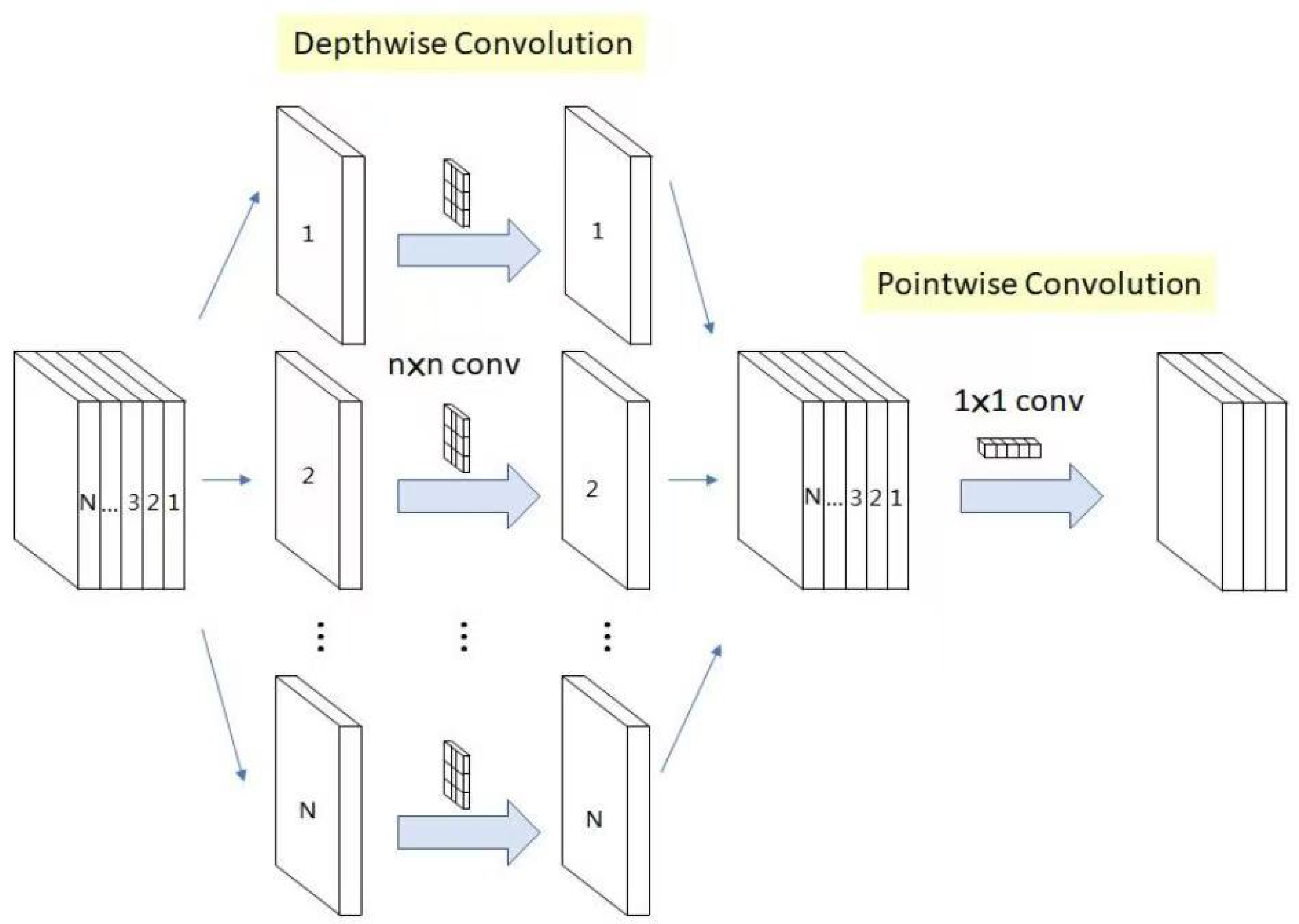
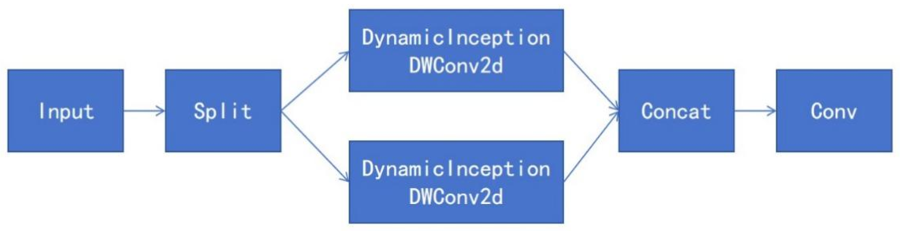
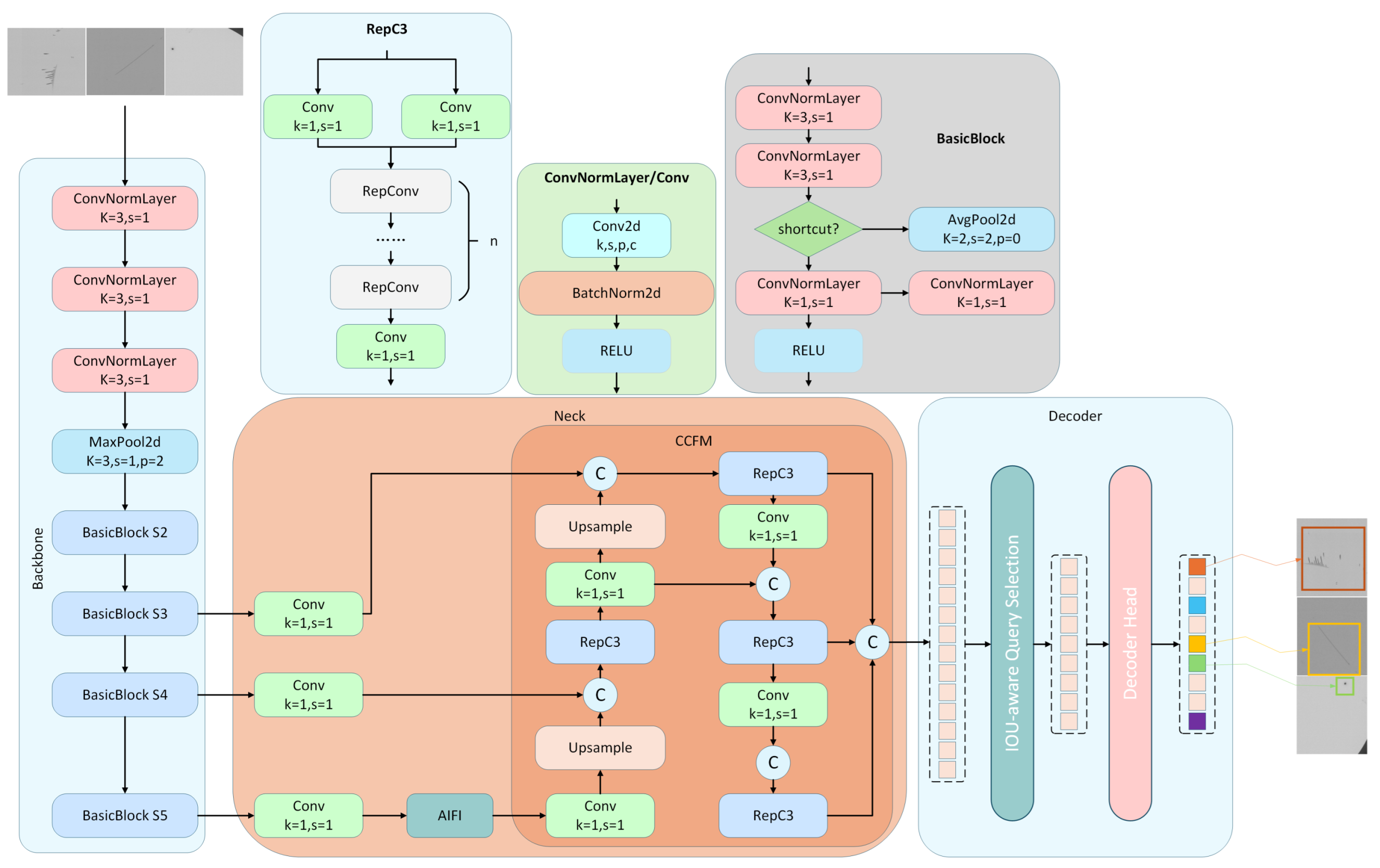
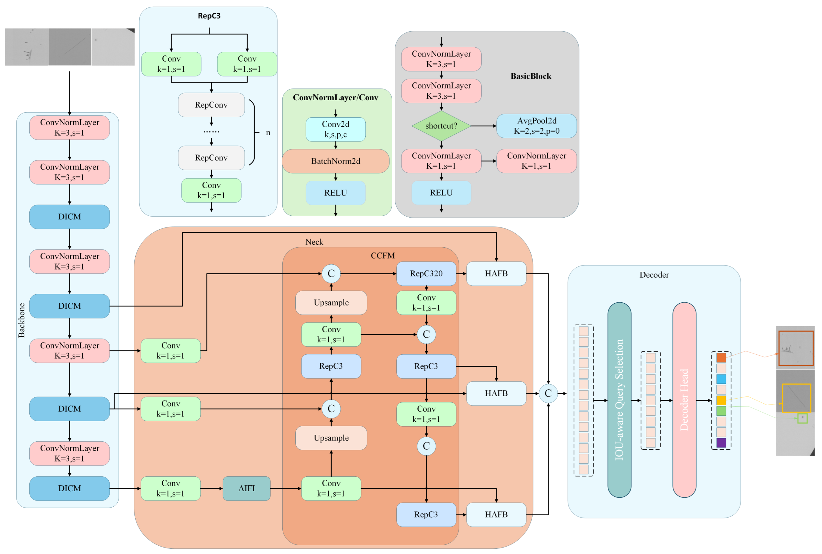
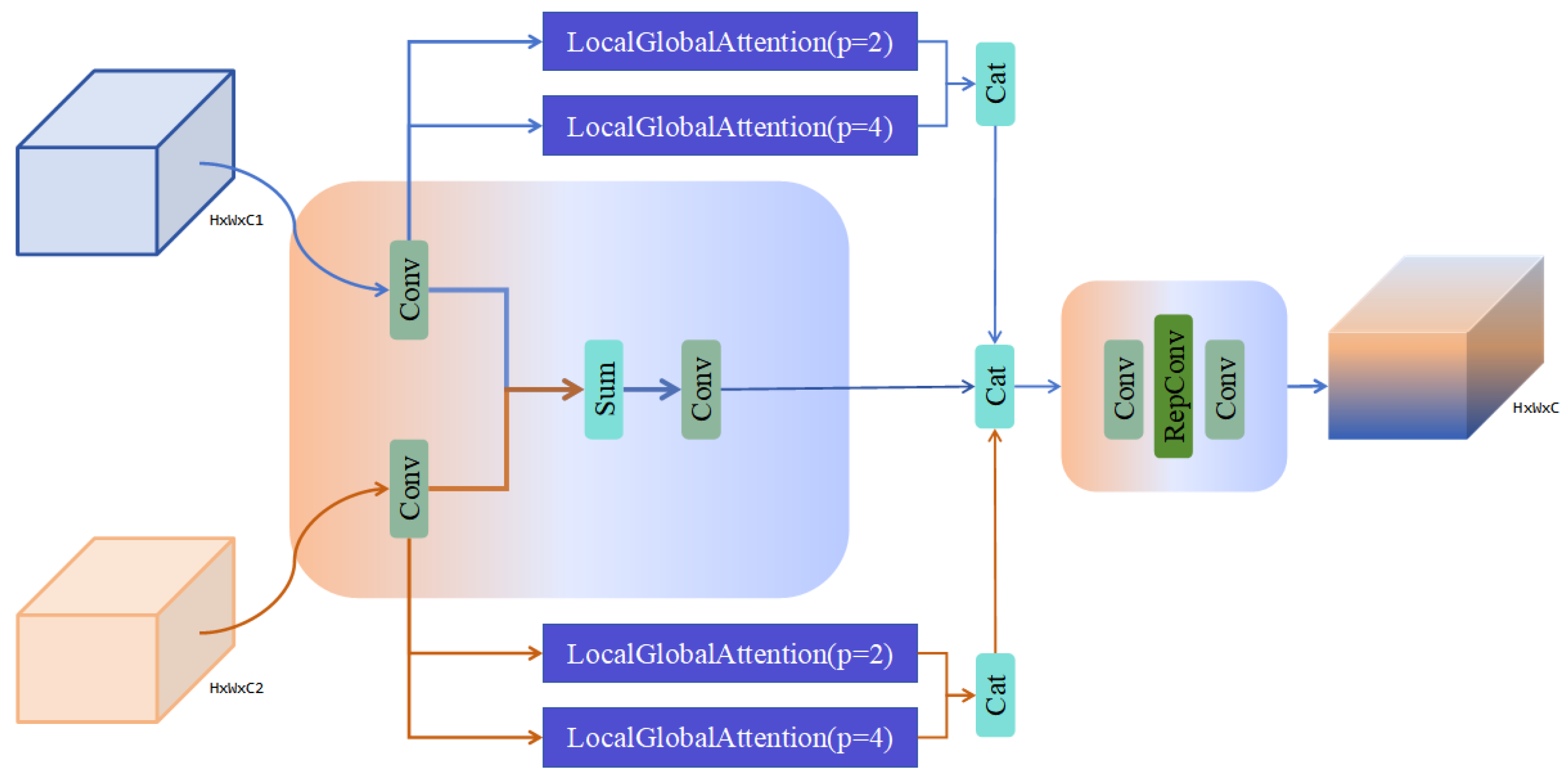
To systematically evaluate the effectiveness of the Dynamic Inception Convolution Module (DICM) and the Hierarchical Attention Fusion Block (HAFB), ablation experiments were conducted based on the benchmark RT-DETR model, and the results are listed in

Table 3. Ablation experiments.

DICM	HAFB	Precision (P)	Recall (R)	mAP@0.5	FPS	Model File Size
		0.78	0.80	0.83	75.29	80.7 MB
✓		0.77	0.81	0.84	72.67	51.6 MB
	✓	0.81	0.83	0.87	78.96	77.5 MB
✓	✓	0.86	0.89	0.88	82.77	78.4 MB

Note: ✓ indicates that the corresponding module is enabled.

.

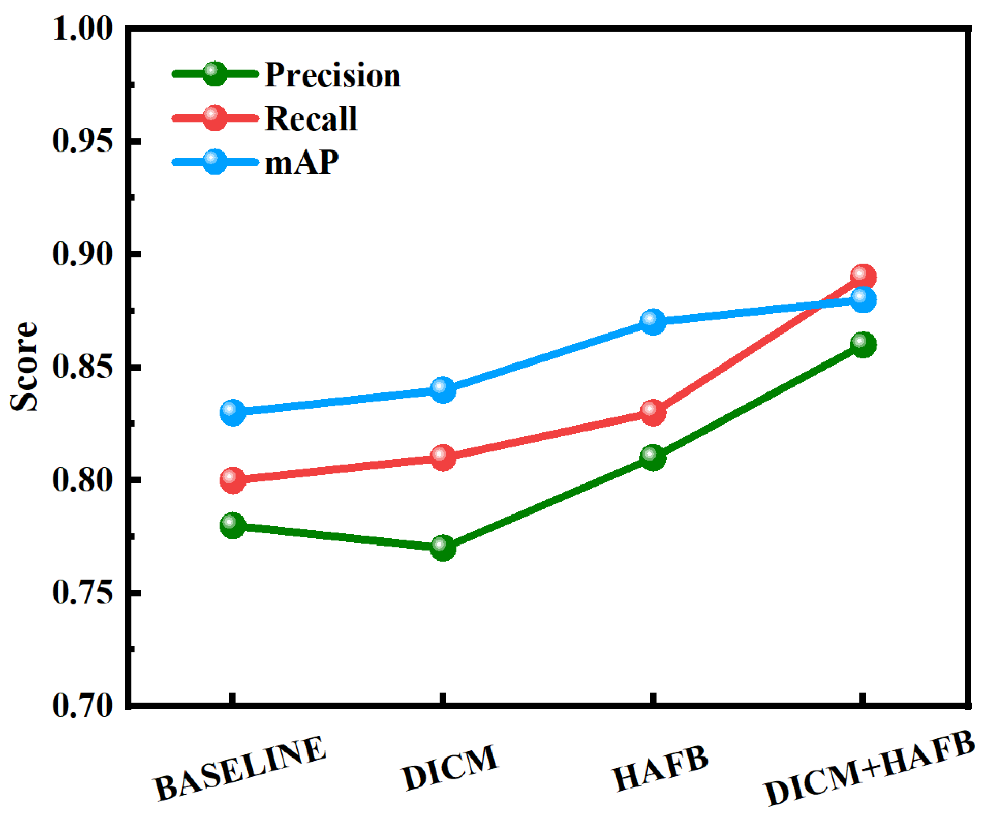
The baseline model, without any enhancement modules, achieved Precision, Recall, and mAP@0.5 values of 0.78, 0.80, and 0.83, respectively, with an FPS of 75.29 and a model size of 80.7 MB, which serves as the reference for subsequent comparison.

When only DICM was introduced, Recall increased from 0.80 to 0.81 and mAP@0.5 improved to 0.84, indicating that DICM enhances defect representation and helps reduce missed detections. However, Precision slightly decreased to 0.77 and FPS dropped to 72.67, suggesting that the strengthened feature modeling also introduced a certain computational burden and false-positive risk. Notably, the model size was reduced to 51.6 MB, a decrease of 36.1% compared with the baseline, demonstrating the advantage of DICM in lightweight design.

When only HAFB was introduced, the model achieved more balanced improvements, with Precision, Recall, and mAP@0.5 reaching 0.81, 0.83, and 0.87, respectively, while FPS increased to 78.96 and the model size slightly decreased to 77.5 MB. These results indicate that HAFB can effectively improve both feature fusion quality and detection efficiency by integrating local details with global semantic information.

When DICM and HAFB were integrated simultaneously, the model achieved the best overall performance. Precision, Recall, and mAP@0.5 reached 0.86, 0.89, and 0.88, respectively, representing improvements of 10.3%, 11.3%, and 6.0% over the baseline model. Meanwhile, FPS increased to 82.77, about 9.9% higher than the baseline, while the model size remained at 78.4 MB, which is close to that of the original model. Compared with the single-module settings, the combined model showed superior performance across all metrics, indicating that DICM and HAFB play complementary roles in feature extraction and feature fusion.

As shown in Figure 9, DICM exhibits clear advantages in lightweight design and feature enhancement, whereas HAFB is more effective in improving accuracy and efficiency. Their combination enables a better balance among detection accuracy, inference speed, and model size.

4.3.2. Comparison of Transfer Learning Experiments

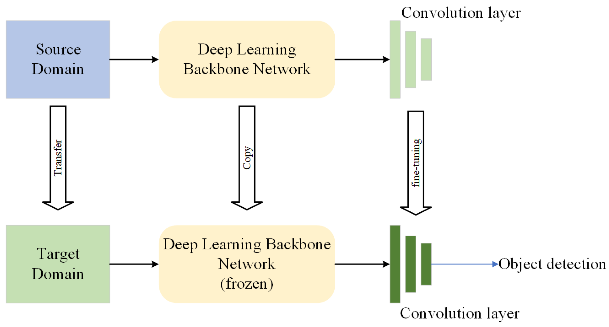
To further verify the effectiveness of transfer learning combined with detection head optimization, comparative experiments were conducted on the target-domain dataset. Model A denotes the configuration without transfer learning, while Model B denotes the configuration with transfer learning and an optimized detection head. The comparison results are listed in

Table 4. Comparison results of transfer learning and detection head optimization.

Model Name	Precision (P)	Recall (R)	mAP@0.5	FPS	Size (MB)
A	0.86	0.89	0.88	82.77	78.43
B	0.87	0.94	0.94	87.62	80.12

.

As shown in Table 4, the overall detection performance is significantly improved after introducing transfer learning and detection head optimization. Compared with Model A, Model B increases Precision from 0.86 to 0.87, Recall from 0.89 to 0.94, and mAP@0.5 from 0.88 to 0.94. Among these metrics, the improvement in Recall is particularly notable, indicating that the improved model is more capable of detecting real defect targets and reducing missed detections, especially for small or weak-texture defects. This result suggests that the optimized model provides better adaptability to complex defect distributions under small-sample conditions.

In terms of comprehensive detection performance, the increase in mAP@0.5 from 0.88 to 0.94 shows that the combination of transfer learning and detection head optimization improves both localization and classification capability. On the one hand, the optimized detection head enhances the flexibility of target prediction; on the other hand, transfer learning enables the model to inherit useful feature representations from the source domain, thereby improving feature extraction efficiency on the target task. The joint effect of these two strategies leads to a clear improvement in overall detection accuracy.

In terms of inference efficiency, Model B achieves 87.62 FPS, which is higher than the 82.77 FPS of Model A, indicating that the improved model still maintains good real-time performance. In addition, the model size only increases slightly from 78.43 MB to 80.12 MB. Although the parameters grow modestly, the gain in detection accuracy and recall is more significant. Therefore, the improved model achieves a better balance among accuracy, recall, real-time performance, and model size.

To further validate the transferability claim and isolate the specific contributions of the transfer learning step across different morphological categories, an additional class-wise ablation experiment was conducted. We compared the model trained from scratch (without pre-trained weights) against the model initialized with source-domain transfer learning across point, line, and planar defect subsets. The results are summarized in

Table 5. Ablation experiment of transfer learning on individual defect subsets.

Defect Type	mAP@0.5 (Scratch)	mAP@0.5 (With Transfer Learning)	Improvement
Point Defect	0.84	0.95	+11.0%
Line Defect	0.90	0.97	+7.0%
Planar Defect	0.87	0.93	+6.0%

.

As the results clearly indicate, the transfer learning strategy yields consistent improvements across all defect subsets. Notably, point defects exhibited the most significant gain in AP@0.5 (from 0.84 to 0.95, an 11.0% improvement). This confirms that the pre-trained weights effectively mitigate the risk of overfitting, providing robust feature initialization for small, discrete targets under small-sample conditions. Furthermore, the performance boosts on linear (+7.0%) and planar defects (+6.0%) demonstrate that the general edge, contour, and complex texture representations learned from the source domain are highly transferable to geometrically complex targets in our target domain. This experiment strongly validates the effectiveness and generalizability of the proposed transfer learning strategy.

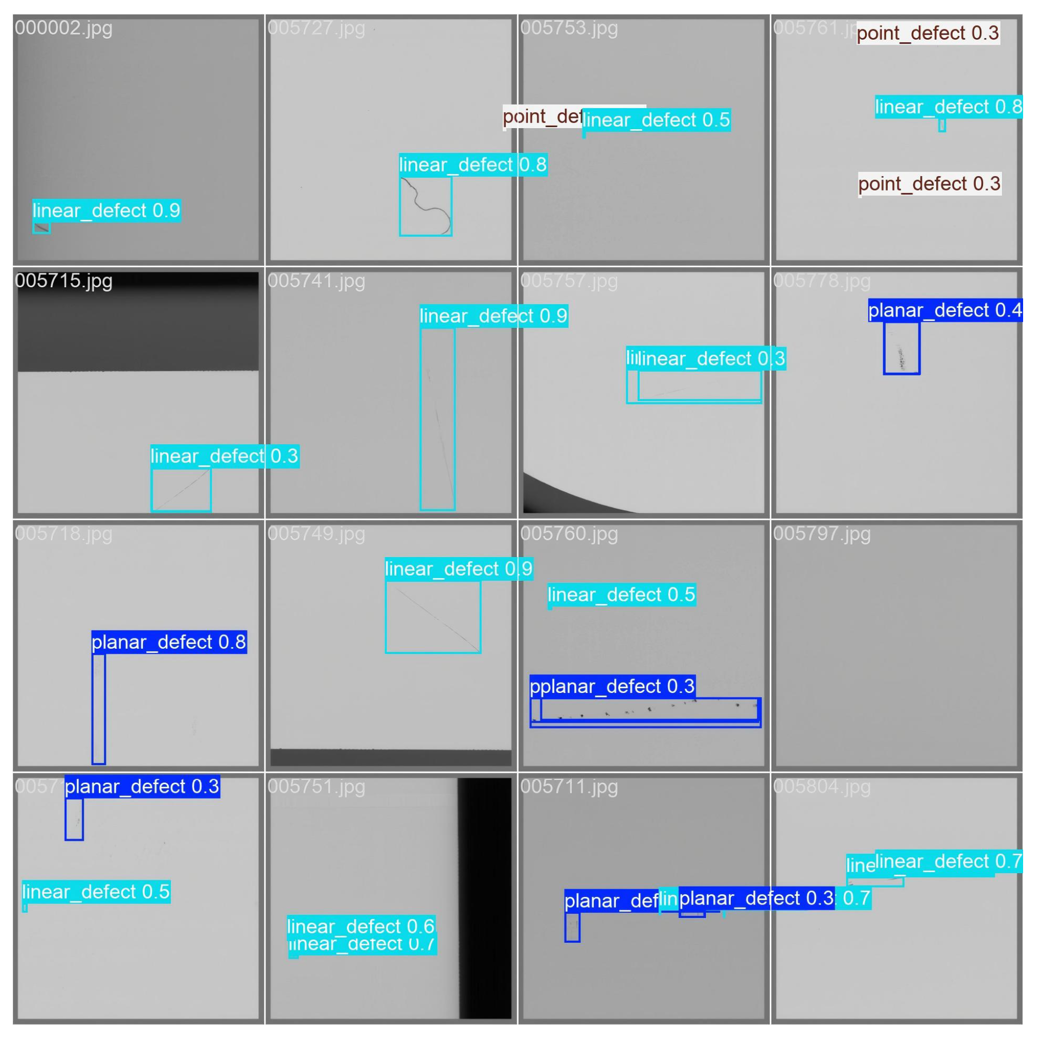
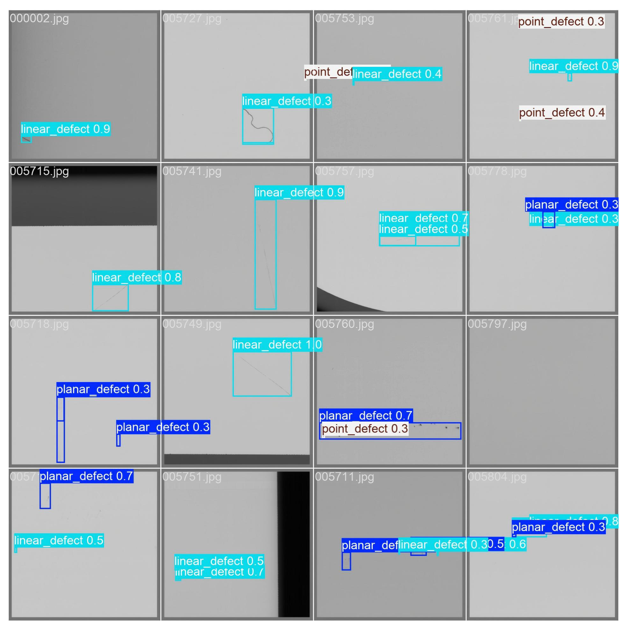
Figure 10 shows the detection results of Model A on the test images. The model can identify some linear defects, but it still has clear limitations in detecting point defects and surface defects. In several fine-textured or complex-background regions, missed detections occur, and some predicted bounding boxes are not well aligned with the actual defect regions. These results indicate that the baseline model still lacks sufficient representation ability for small defects and complex backgrounds.

Figure 11 shows the detection results of the improved Model B on the same test images. Compared with Model A, Model B exhibits more stable detection across different defect categories, especially for point defects and surface defects. The predicted boxes are more accurately aligned with the target boundaries, and missed detections are significantly reduced even under complex textured backgrounds. These observations further confirm the effectiveness of transfer learning and detection head optimization in improving small-defect detection performance.

4.3.3. Heatmap Analysis

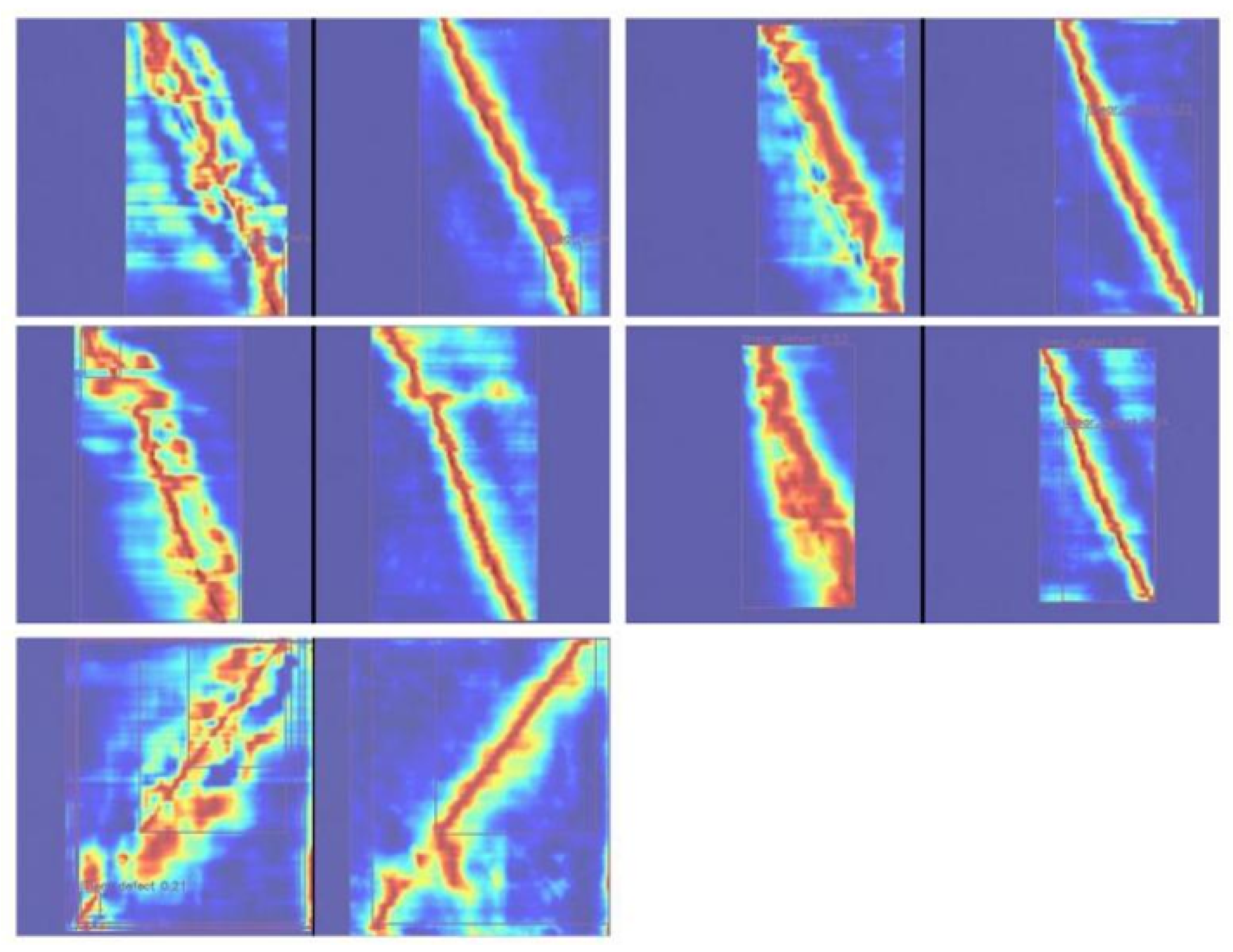
To further compare the feature response differences between the original RT-DETR model and the improved model, heat map visualization analysis was conducted. Five representative samples with obvious response differences were selected, as shown in Figure 12.

Overall, the improved model exhibits more concentrated and higher-intensity responses in defect regions, and its activation areas better coincide with the actual defect locations. In contrast, the original RT-DETR model shows more dispersed responses and stronger background interference, and some samples present response offsets or incomplete coverage.

For fine-grained defects such as microscopic scratches and point-like defects, the difference between the two models is more evident. The original model shows weak or blurred responses and fails to effectively highlight defect regions, whereas the improved model produces clearer high-response clusters in micro-defect areas. This indicates that the proposed improvements enhance the model’s ability to capture local details and improve small-defect perception.

For strip-shaped crack defects, the heat maps of the improved model present a more continuous and stable response distribution along the defect direction, which is closer to the actual defect contour. In addition, under complex backgrounds or irregular defect patterns, the improved model focuses more on defect regions while suppressing interference from background textures and illumination variations. These results demonstrate that the improved model achieves better feature selection, stronger anti-interference ability, and higher discriminative power than the original RT-DETR model.

4.3.4. Confusion Matrix Analysis

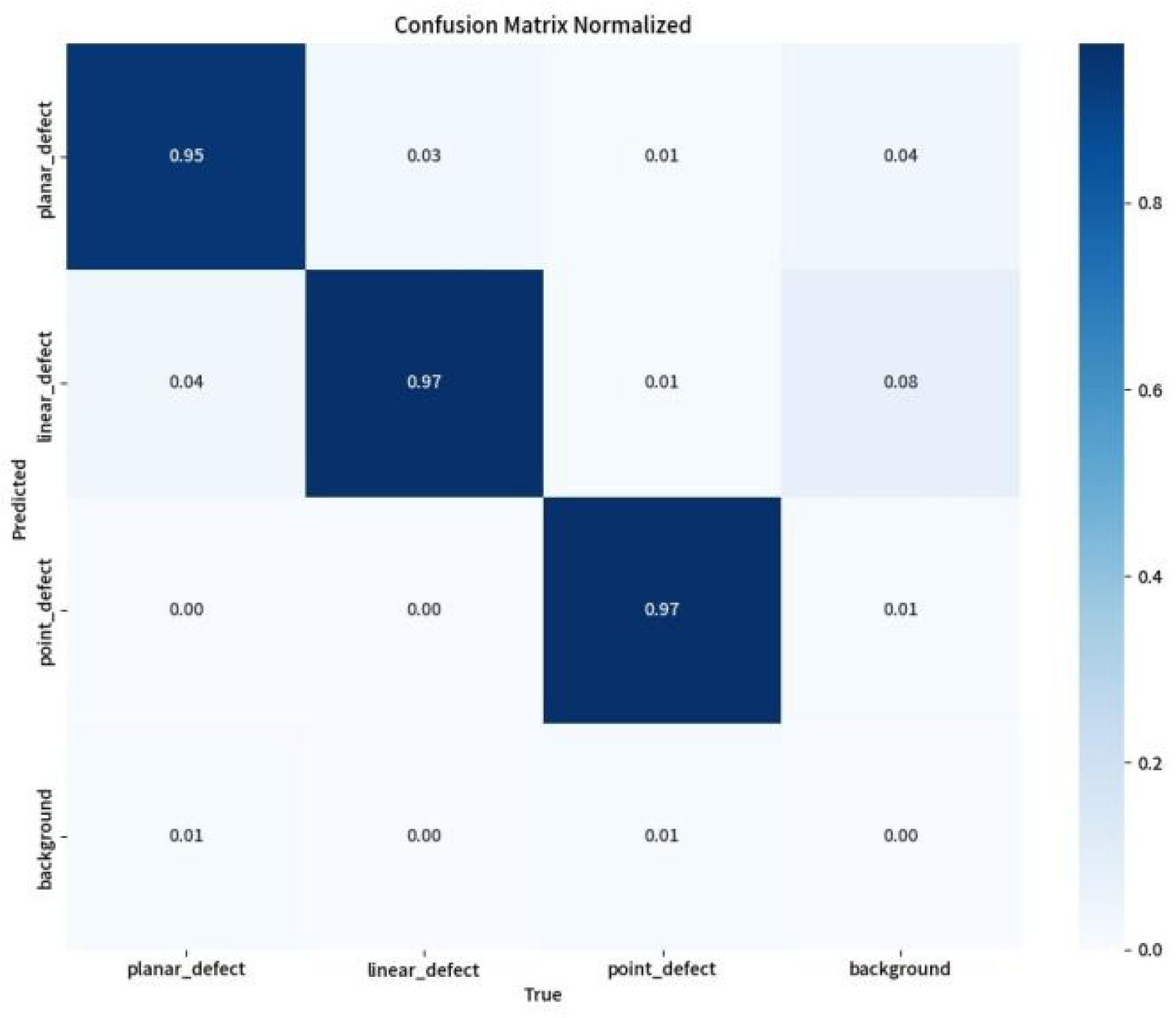
To further evaluate the classification performance and inter-class discrimination ability of the improved model for different defect categories, a confusion matrix was constructed based on the test set results, as shown in Figure 13. In the matrix, the horizontal axis represents the true labels, the vertical axis represents the predicted labels, the diagonal elements denote correct classification proportions, and the off-diagonal elements indicate misclassification relationships.

Overall, most samples are concentrated along the diagonal, indicating that the improved model achieves high classification accuracy and strong category discrimination across the three defect types. Compared with the original model, the improved RT-DETR exhibits more accurate predictions for all categories, which further demonstrates the effectiveness of the optimization strategy.

For planar defects, the classification accuracy reaches 0.95. Since these defects usually exhibit relatively large spatial distribution and obvious texture characteristics, the model can effectively capture their regional features. Only a small proportion of planar defects are misclassified as linear defects or point defects, which is mainly caused by local linear boundary structures in some planar defects.

For linear defects, the classification accuracy reaches 0.97, which is one of the best among the three categories. This is mainly because linear defects have strong directional continuity and prominent geometric characteristics, making them easier to learn during feature extraction. A few samples are misclassified as planar defects, mostly because some wide crack-like defects show local planar expansion patterns and thus increase classification difficulty.

For point defects, the model also achieves a classification accuracy of 0.97, indicating strong fine-grained feature extraction capability. The confusion with other categories is minimal, which shows that the improved model performs well in representing small and discrete defect patterns. This result also verifies the effectiveness of the proposed optimization strategy in improving small-defect perception.

From the off-diagonal regions, a small number of defect samples are still misclassified as background. For example, a minor proportion of linear defects are predicted as background, mainly because some defect features are weak and show limited grayscale or texture differences from the surrounding area. In addition, illumination variation and reflection interference in industrial environments may further affect feature extraction. Nevertheless, the proportion of such errors remains low and has limited influence on overall model performance.

In summary, the confusion matrix shows that the improved RT-DETR model maintains high consistency and stability across different defect categories. The main confusion occurs between linear defects and planar defects, whereas point defects show very limited overlap with other categories. These results further confirm that the proposed method improves category discrimination and anti-interference ability in solar vacuum glass collector tube defect detection. 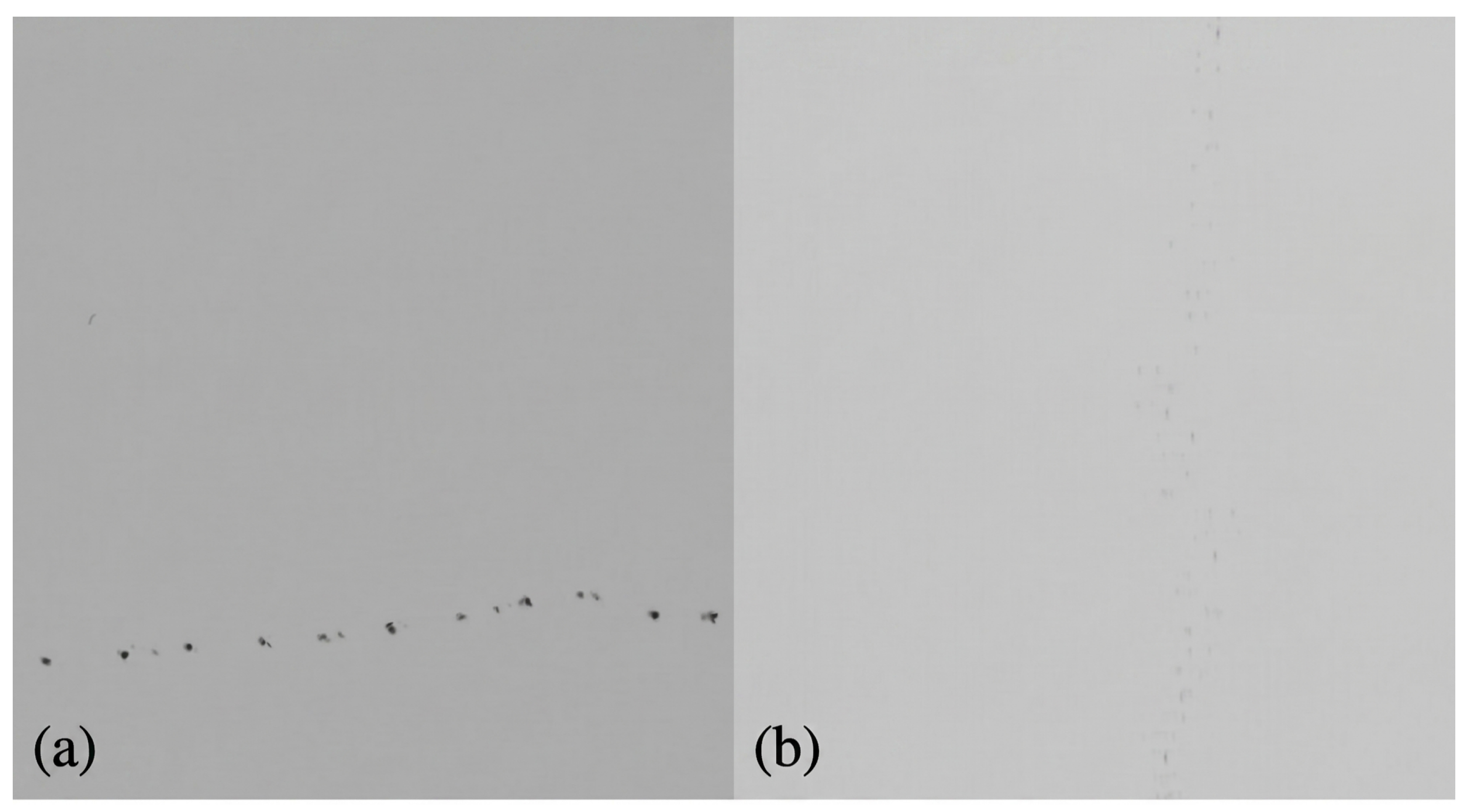To intuitively illustrate the specific geometric ambiguities contributing to these misclassifications within the confusion matrix, Figure 14 presents typical cases where linear and planar defects are confused.

Geometrically, the proposed model occasionally struggles with these two classes due to the inherent cylindrical curvature of the vacuum tubes and the resulting perspective projections. As shown in Figure 14a, a series of discrete point-like defects may align in a way that, when viewed from certain angles or compressed by the tube’s curvature, resembles a continuous linear feature. This topological similarity can mislead the model into classifying a cluster of small defects (planar-like) as a single linear defect.

Conversely, as depicted in Figure 14b, extremely faint and blurred linear scratches often lack distinct edge features. Under low-contrast conditions, the blurred texture of these scratches can lose its directional information, causing the model to perceive the defect as a vague, two-dimensional region rather than a clear line. These geometric and optical factors explain the higher off-diagonal values between the linear and planar categories observed in the confusion matrix.

4.3.5. Comparison with Mainstream Algorithm Models

To evaluate the comprehensive performance of the proposed model for solar vacuum glass collector tube defect detection, comparative experiments were conducted on the self-built dataset using multiple mainstream object detection algorithms. The compared models included Faster R-CNN, YOLOX-S, PP-YOLOE-S, EfficientDet-D1, YOLOv8, DINO-DETR, and RT-DETR, together with two reference methods from the literature. All models were trained and tested under the same hardware environment and dataset settings to ensure fair comparison. The corresponding results are listed in

Table 6. Comparative Test with Mainstream Algorithms.

Model	Training Rounds	Precision (P)	Recall (R)	mAP@0.5	FPS	Size (MB)
[17]	100	0.97	0.96	0.97	41.00	35.13
[18]	200	0.83	0.85	0.81	97.66	-
YOLOX-S	200	0.81	0.79	0.78	95.75	95.44
PP-YOLOE-S	200	0.72	0.77	0.71	91.23	92.65
EfficientDet-D1	200	0.79	0.74	0.74	57.44	59.32
DINO-DETR	100	0.74	0.72	0.71	44.84	73.36
Faster R-CNN	200	0.76	0.79	0.80	45.25	125.98
YOLOv8	200	0.80	0.81	0.84	85.67	95.02
RT-DETR	100	0.78	0.80	0.83	75.32	80.73
MobileViT	200	0.82	0.80	0.81	62.45	22.40
YOLOv10-S	200	0.89	0.87	0.88	81.31	31.50
Ours	100	0.96	0.95	0.95	83.21	82.36

.

As shown in Table 6, the proposed model achieves Precision, Recall, and mAP@0.5 of 0.96, 0.95, and 0.95, respectively, which are markedly higher than those of most comparison models. Compared with the original RT-DETR, whose mAP@0.5 is 0.83, the improved model shows clear gains in all major accuracy metrics, indicating that the proposed improvements effectively enhance feature representation and defect discrimination capability.

Among the compared methods, Faster R-CNN shows relatively stable accuracy, but its inference speed is limited to 45.25 FPS, which is insufficient for real-time industrial deployment. Lightweight detectors such as YOLOX-S and PP-YOLOE-S achieve FPS values above 90, but their mAP@0.5 values are only 0.78 and 0.71, respectively, indicating limited performance in small-sample and complex defect scenarios. For Transformer-based methods, DINO-DETR achieves an mAP@0.5 of 0.71, while the original RT-DETR reaches 0.83, showing better overall suitability for this task. The proposed model further improves upon RT-DETR and achieves a better balance between accuracy and real-time performance.

To further demonstrate the superiority of the proposed method, we incorporated MobileViT and YOLOv10-S as additional benchmarks in Table 6. While MobileViT offers extreme model compactness, its pure Transformer-based architecture struggles to extract fine-grained local features from small-sample glass defects, resulting in a lower mAP@0.5 of 0.81. On the other hand, although YOLOv10-S achieves the highest inference speed (98.20 FPS), its general-purpose feature extraction backbone lacks specific mechanisms to suppress complex background noise and reflections inherent in solar vacuum tubes. In contrast, our improved RT-DETR leverages the DICM and HAFB modules to achieve a more robust balance, reaching an mAP@0.5 of 0.95 while maintaining real-time performance (83.21 FPS).

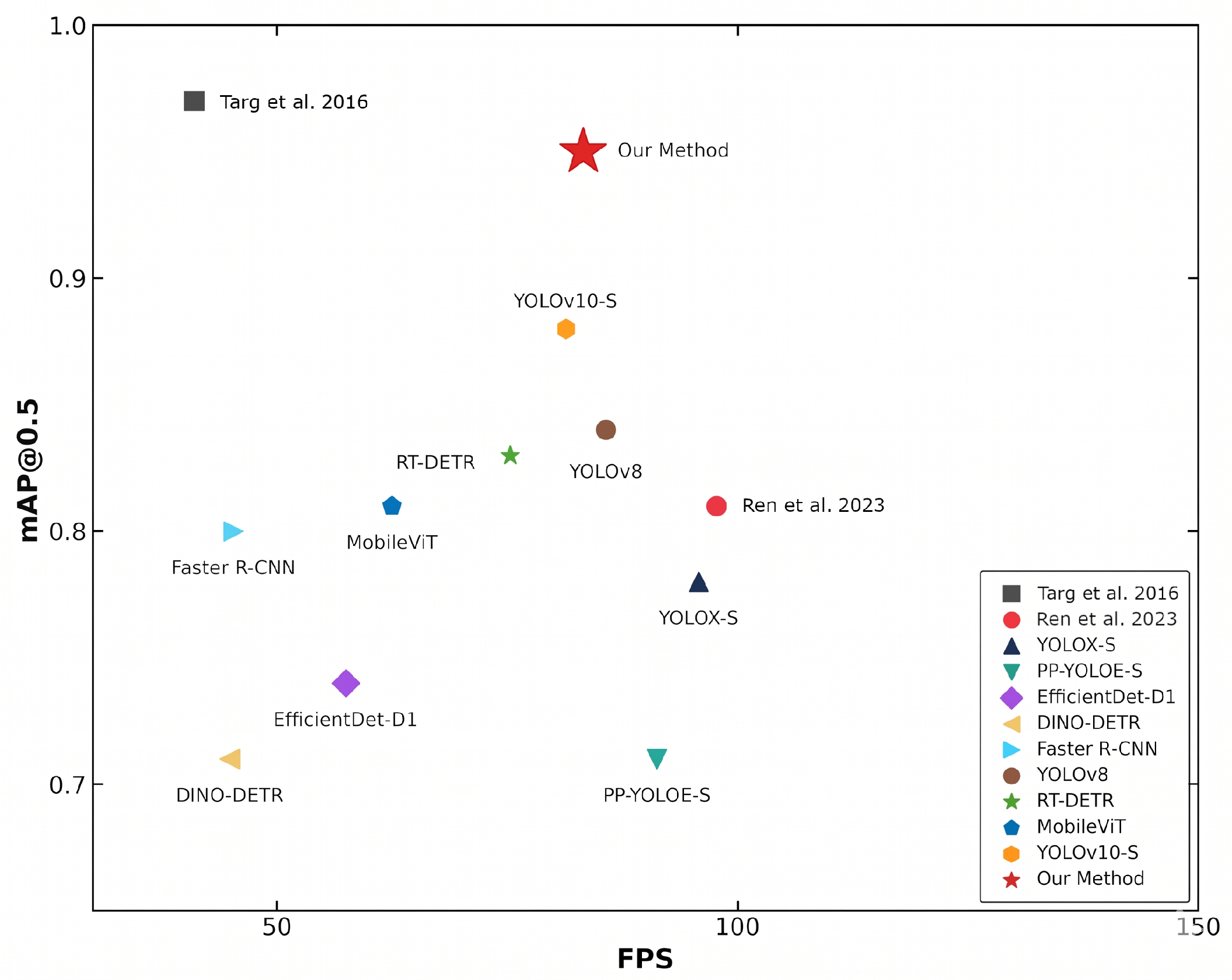
In terms of efficiency, the proposed model reaches 83.21 FPS with a model size of 82.36 MB. Although its speed is slightly lower than that of some lightweight YOLO models, it remains competitive among high-accuracy detectors. As shown in Figure 15, the proposed model is positioned in the upper-right region of the mAP-FPS scatter plot, indicating that it maintains both high detection accuracy and favorable real-time performance. These results demonstrate that the proposed method achieves a strong trade-off between precision and computational efficiency.

It is worth noting that the proposed model achieves a substantial improvement in mAP@0.5 (from 0.83 to 0.95) compared to the baseline RT-DETR. This significant gain is a cumulative result of multi-stage optimization rather than data leakage or overfitting. As shown in the ablation study (Table 3), structural optimizations (DICM and HAFB) alone improved the mAP to 0.88. The subsequent jump to 0.95 is strictly attributed to the high-quality transfer learning strategy guided by cosine similarity, which selectively filtered the most semantically relevant source-domain samples (threshold 0.80) to maximize pre-training efficiency while reducing negative transfer. To ensure experimental integrity, strict physical isolation was maintained between the training, validation, and testing sets, and shallow feature layers were frozen during fine-tuning to act as a regularizer against overfitting in small-sample scenarios.

4.4. Demonstration of Actual Results

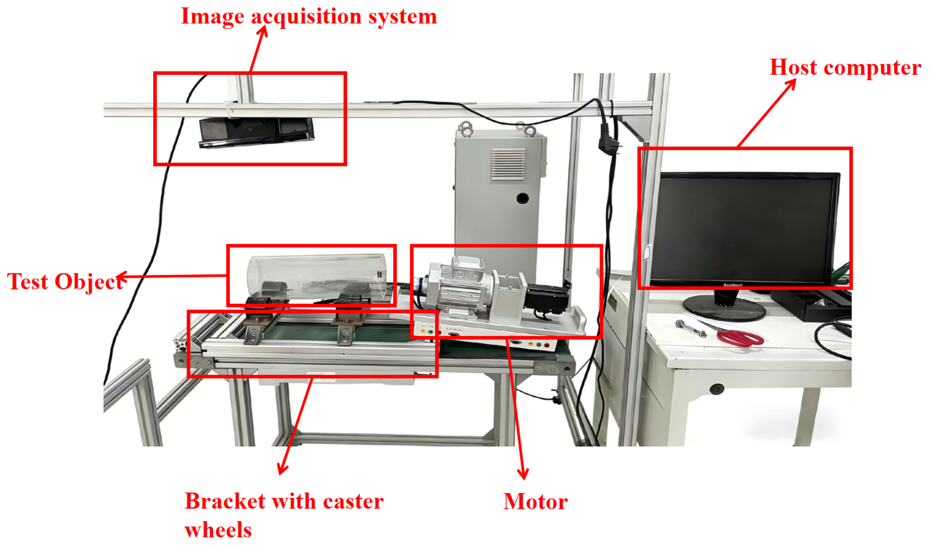
After completing system construction and model deployment, a practical experimental platform was established to evaluate the real-world applicability of the proposed method, as shown in Figure 16. The system mainly consists of an image acquisition module, a motion control module, and a host computer processing module. The camera is fixed above the platform to capture real-time images of solar vacuum glass collector tubes, and a stable light source is used to ensure imaging consistency. During operation, the collector tube is placed on a roller support, and the right-side motor drives continuous rotation to achieve full-surface scanning and avoid detection blind spots. The captured images are transmitted to the host computer, where preprocessing and defect detection are performed by the optimized RT-DETR model, and the final results are displayed visually on the interface.

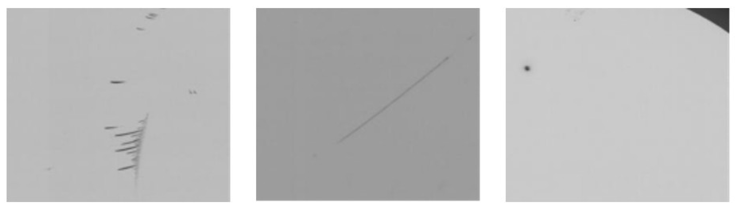
To further validate the detection performance in practical industrial scenarios, multiple online detection experiments were conducted on real solar vacuum glass collector tubes, and statistical analysis was performed for different defect categories. The results show that the system achieves high recognition accuracy for all three representative defect types. Specifically, among 300 point defects, 295 were correctly detected, corresponding to a detection rate of 98.33%. Among 200 linear defects, 199 were detected, yielding a detection rate of 99.50%. For 100 planar defects, 98 were correctly identified, corresponding to a detection rate of 98.00%, as listed in

Table 7. Statistical Analysis of Actual Test Results.

Defect Type	Real Quantity	Detection Count	Detection Rate
point defect	300	295	0.98
line defect	200	199	0.99
planar defect	100	98	0.98

.

Overall, the system achieves detection rates above 98% for all three defect categories, indicating good accuracy and stability in practical deployment. Linear defects show the highest detection rate, suggesting that the model has strong capability in extracting slender structural features. Point defects also achieve satisfactory performance, confirming the effectiveness of the proposed method for small-scale defect perception. In comparison, the detection rate of planar defects is slightly lower, mainly because their irregular morphology makes them more susceptible to illumination variation and background texture interference.

Further analysis of the undetected samples shows that missed detections mainly occur in the following situations: defects with very small dimensions or low grayscale contrast provide insufficient feature representation; strong reflections or uneven local illumination reduce the contrast between the defect region and the background; and some linear defects have blurred edges, which causes slight localization deviations.

To evaluate real-time performance in industrial scenarios, inference speed tests were further conducted using FPS as the evaluation metric. Under GPU-accelerated continuous detection, the system achieves an average speed of 70.79 FPS, which satisfies the real-time requirements of industrial online inspection. Even in scenarios with multiple coexisting defects, the system maintains stable inference performance without significant degradation.

5. Conclusions

To address the challenges of limited small-sample data, insufficient detection accuracy, and weak robustness in complex environments for solar vacuum glass collector tube defect detection, this study proposes a small-sample defect detection method based on RT-DETR. Transfer learning is adopted to alleviate overfitting caused by limited target-domain data, while data augmentation is used to improve sample diversity and model generalization. In terms of model architecture, the proposed method enhances RT-DETR from two aspects: DICM is introduced into the backbone to improve the representation of complex textures and fine-grained defects and HAFB is embedded into the neck to strengthen multi-scale feature fusion and small-defect perception. Experimental results show that the improved model achieves clear advantages over the baseline RT-DETR and several mainstream detection models in terms of Precision, Recall, mAP@0.5, and practical detection performance, while maintaining favorable real-time capability and model compactness. In practical deployment, the detection system achieves over 98% detection rates for three typical defect categories and maintains an average speed of 70.79 FPS, demonstrating good applicability in industrial online inspection.

Despite the promising results achieved in this study, several challenges remain for real-world industrial deployment. First, while our experimental platform utilized stable illumination, practical environments often suffer from varying lighting conditions. Under extreme high-lighting, the highly reflective curved surface of the glass tubes causes localized specular overexposure, which obscures the morphological boundaries of minor defects and inevitably leads to false negatives. Conversely, low-lighting conditions diminish the grayscale contrast between defects and the background, hindering effective semantic feature extraction. Future work must incorporate adaptive illumination compensation mechanisms to enhance environmental robustness.

Second, the acquisition of specialized, fully annotated industrial datasets remains prohibitively expensive. To reduce reliance on manual annotation and improve transferability across different operating environments, future research will explore semi-supervised learning (SSL) paradigms. By leveraging pseudo-labeling and consistency regularization on the massive streams of unlabeled data generated daily on production lines, the model’s feature space can be continuously refined without incurring additional costs. This can be further complemented by expanding the dataset to include more defect categories and cross-scenario samples.

Third, integrating Physics-Informed Machine Learning (PIML) offers a highly efficient pathway to enhance predictive performance. Solar vacuum collector tubes possess distinct geometric and optical properties, such as cylindrical curvature and high reflectivity. Rather than relying solely on data-driven approaches, PIML can embed optical reflection priors (e.g., Fresnel equations or ray-tracing physical laws) directly into the neural network’s loss function, penalizing predictions that violate physical constraints. This physics-driven approach, potentially combined with multimodal information (such as infrared or polarized images), can further enhance robustness under complex conditions. Finally, exploring model compression, knowledge distillation, and hardware-friendly operators will remain essential to maximize deployment efficiency on edge devices.