Study on Damage Evolution and Acoustic Emission Response Characteristics of Loaded Saturated Sandstone Under Different Freeze–Thaw Temperature Differences

Abstract

In cold-region open-pit mine slopes, damage accumulation and mechanical deterioration induced by in situ stress and seasonal freeze–thaw alternation can easily trigger sudden instability. To investigate the effects of temperature difference under coupled constant loading and freeze–thaw action on the mechanical response and failure precursors of rock, based on the self-developed TCDR-I temperature–stress coupled testing system, uniaxial compression tests and real-time acoustic emission monitoring were conducted on water-saturated sandstone under a constant load of 1.4 MPa and multiple freeze–thaw temperature gradients. The mechanical behavior of freeze–thawed water-saturated sandstone and the acoustic emission characteristics during failure were analyzed. Combined with critical slowing down theory, the failure precursor characteristics of water-saturated sandstone under freeze–thaw action were investigated, and the internal mechanism of damage accumulation and defect evolution under the coupled effects of constant load and freeze–thaw temperature difference was revealed. The results show that, with increasing freeze–thaw temperature difference, the number of cracks and crack ratio in the loaded water-saturated sandstone gradually increased, whereas the compressive strength, elastic modulus, and total strain energy gradually decreased. After freeze–thaw treatment at −40 to 20 °C, the compressive strength, elastic modulus, and total strain energy decreased by 19.24%, 13.72%, and 44.77%, respectively, compared with those of the unfrozen–thawed specimens. During specimen failure, the dominant crack type gradually shifted from shear cracking to tensile cracking. The acoustic emission b-value and precursor points identified from multiparameter variance can both be used as criteria for predicting specimen failure. The warning lead time increased with increasing freeze–thaw temperature difference. After freeze–thaw treatment at −40 to 20 °C, the predicted failure times based on these two indicators preceded the actual failure time by 11.05 s and 16.19 s, respectively. The findings provide a theoretical basis for the early warning of sudden disasters in rock masses in cold-region engineering.

1. Introduction

Cold regions are typically characterized by prolonged low temperatures, pronounced seasonal freezing, and frequent freeze–thaw cycles. Open-pit mines in China are predominantly located in the northwestern regions [1]. As shallow open-pit ore bodies extend deeper, they form numerous steep-sided, deep-concave slopes, Coupled with the seasonal and diurnal temperature variations in these cold regions, the rock masses within these slopes repeatedly undergo freeze–thaw cycles [2,3]. Under the long-term coupled effects of static loading and freeze–thaw cycles, rock masses experience a complex physicochemical evolution. This process compromises their structural integrity, subsequently leading to a reduction in bearing capacity and a degradation of mechanical properties, which significantly impacts the safety and stability of slopes [4,5]. Identifying the precursor characteristics of fracture evolution in the early stages of damage can effectively control damage propagation and enhance slope safety. Therefore, investigating rock damage mechanics and fracture precursor characteristics under coupled loading and freeze–thaw conditions is of significant practical engineering importance for disaster prevention in open-pit mines located in high-altitude cold regions.

Scholars both domestically and internationally have conducted extensive research on the degradation of rock physical properties and the precursors to fracturing under freeze–thaw cycling. Xu et al. and Tan et al. conducted uniaxial and triaxial compression tests on freeze–thawed rocks and found that with increasing cycle numbers, the uniaxial compressive strength and elastic modulus of the rocks showed a declining trend, with most rock specimens exhibiting flake-like and crack-type failure [6,7]. Jia et al. investigated the temporal and temperature-dependent behavior of rocks with varying fracture lengths, widths, and lithologies during freeze–thaw cycles, establishing the variation patterns of freeze–thaw deformation characteristics in saturated fractured rocks. In the context of fracture precursors [8], Du et al. examined the mechanical behavior of marble and sandstone under biaxial confinement and proposed a precursor warning method based on the b-value of acoustic emission [9]. Zhao et al. studied the acoustic emission behavior in An’ying rock under varying stress paths, identifying patterns in acoustic emission b-values as precursors to rock failure [10]. Cui et al. analyzed acoustic emission characteristics during specimen loading, utilizing b-values as failure precursors [11]. Niu et al. suggested that high concentrations of acoustic emission parameters RA and AF serve as early warning signals for imminent failure in red sandstone [12]. Dong et al. investigated the qualitative relationship between rock instability precursors and principal stress directions, concluding that both the acoustic emission event rate and wave velocity serve as precursor indicators for rock sample instability [13]. Zhang et al. identified precursor information related to rock damage and crack propagation by analyzing strain field characteristics and ultrasonic attenuation patterns during rock deformation and failure, thereby providing a basis for predicting rock fracture and instability [14]. Liu et al. employed acoustic emission techniques to capture precursory signals of fracture in freeze–thaw specimens, identifying synchronous, substantial increases in both acoustic emission ringing counts and cumulative energy as precursors to specimen failure and instability [15]. Wu et al. conducted experimental studies on the acoustic emission characteristics during uniaxial compression of sandstone, metagranite, granite, and limestone [16]. They observed that the precursor signal for all four specimens prior to peak stress was characterized by an initial surge in cumulative acoustic emission ringing counts followed by a period of quiescence. Synthesizing the aforementioned scholarly research, it becomes evident that the physical parameter degradation of specimens induced by freeze–thaw cycles fundamentally reflects the continuous accumulation of internal damage. This damage evolution is characterized during loading by the premature emergence and significant amplification of fracture precursors such as acoustic emission, further revealing a correlation between the physical-mechanical strength deterioration of freeze–thaw specimens and fracture precursors.

Previous studies have considered the effects of freeze–thaw cycles, temperature, and other factors on the freeze–thaw behavior of rocks, thereby reflecting, to some extent, the complex occurrence environment of rock masses in cold regions. In fact, slope rock masses in cold regions are subjected not only to freeze–thaw cycling but also to the long-term action of in situ stress. Existing studies have mainly focused on the damage deterioration of rocks under unloaded freeze–thaw conditions, whereas the degradation of mechanical properties, energy evolution, and failure precursor responses of rocks under the coupled effects of constant load and different freeze–thaw temperature differences remain insufficiently understood. Therefore, in this study, a self-developed TCDR-I temperature–stress coupled testing system and an acoustic emission monitoring system were used to conduct uniaxial compression tests and real-time acoustic emission monitoring tests on water-saturated sandstone subjected to the coupled effects of constant load and different freeze–thaw temperature differences. The degradation characteristics of mechanical parameters and the energy evolution of sandstone after freeze–thaw cycling under different temperature differences were comparatively analyzed. Based on the theory of critical slowing down, the failure precursor characteristics of water-saturated sandstone under loading were investigated, and the microscopic mechanism of damage evolution under the coupled effects of constant load and freeze–thaw temperature difference was clarified. The results provide a theoretical basis for stability monitoring and safety assessment of slope rock masses in open-pit mines in cold regions.

2. Experimental Design

2.1. Specimens and Preparation

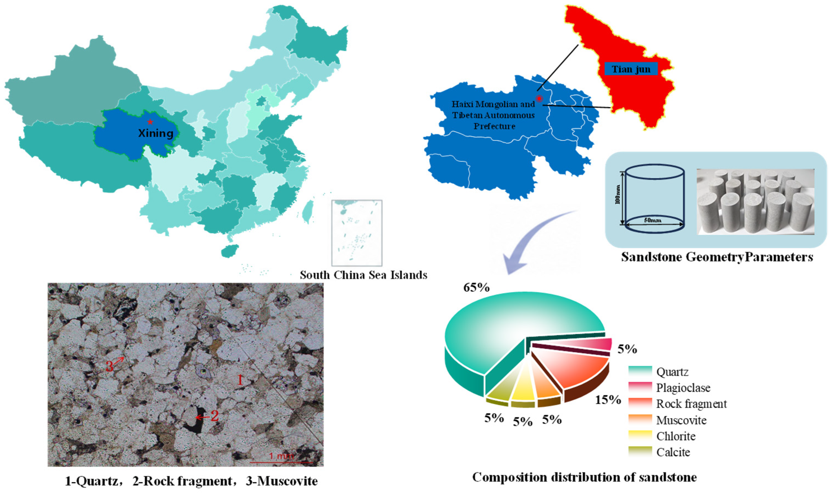
The study area is located in the Juhugeng mining area of the Muli Coalfield on the northeastern margin of the Qinghai-Tibet Plateau, within Tianjun County, Haixi Mongol and Tibetan Autonomous Prefecture, Qinghai Province. Situated in the high-altitude zone of the central Qilian Mountains, the area has an elevation ranging from 3800 to 4200 m, and its geomorphology is predominantly characterized by plateau periglacial landforms [17]. The mineral composition of the sandstone specimens primarily consists of quartz (65%), rock fragments (15%), plagioclase (5%), muscovite (5%), chlorite (5%), and calcite (5%). The minerals are cemented by intergrowths of calcite, ferruginous, and siliceous materials. Overall, the rock sample exhibits a massive texture with a fine-to coarse-grained sandy structure.

The sandstone samples for this study were collected from the Juhugeng mining area within the Muli Coalfield in Qinghai Province, as indicated in Figure 1. The sandstone specimens were processed according to the standards set by the International Society for Rock Mechanics. The prepared specimens were standard cylindrical samples measuring φ50 mm × 100 mm [18]. Both ends of each rock specimen were ground to ensure an end-face parallelism tolerance of less than 0.05 mm. To minimize the impact of sample variability on the test results, ultrasonic velocity meters were used to measure wave velocities. Only samples with similar velocities and dimensions were selected for further analysis. For each test condition, three replicate specimens were prepared to ensure the reliability and reproducibility of the experimental results. Therefore, a total of 15 specimens were prepared for the five test conditions. The basic parameters of the specimens are presented in

Table 1. Test rock sample parameters.

Test Specimen	Weight /g	Diameter /mm	Height /mm	Wave Velocity /(km·s−1)	Bulk Density/kN·m−3
A1	484.9	49.0	101.0	3.769	24.96
A2	482.4	49.1	100.6	3.731	24.83
A3	483.1	49.3	100.9	3.714	24.59
B1	487.2	49.0	100.8	3.488	25.13
B2	488.0	49.0	100.8	3.714	25.17
B3	481.4	49.0	100.5	3.713	24.91
C1	479.2	49.1	99.7	3.537	24.89
C2	488.5	49.2	101.0	3.472	24.94
C3	483.6	49.0	100.5	3.605	25.02
D1	482.8	49.2	99.8	3.578	24.95
D2	487.6	49.1	100.7	3.658	25.07
D3	484.3	49.0	101.4	3.712	24.83
E1	483.4	49.0	101.0	3.545	24.89
E2	485.9	49.0	100.2	3.587	25.21
E3	484.2	49.0	100.4	3.569	25.08

.

2.2. Test System

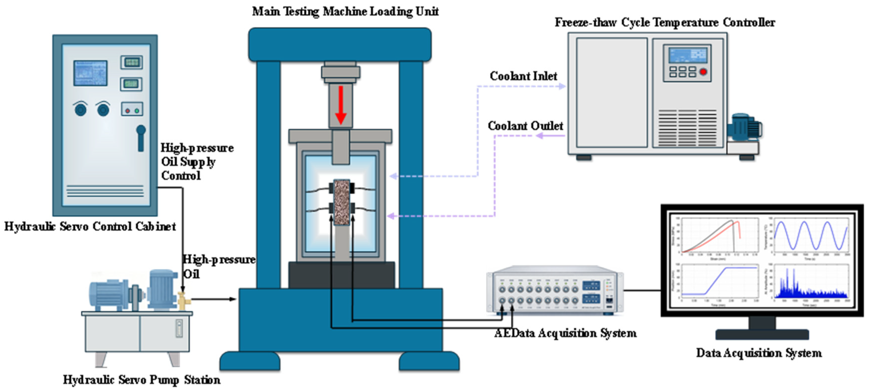
(1) To simulate and monitor the damage evolution of rock under the combined effects of constant axial loading and freeze–thaw cycles with varying temperature differences, a self-developed temperature–stress coupled testing system (TCDR-I) was specifically developed for this study [19]. The independently developed system consists of four main components (Figure 2):

Axial Stress Loading System. This component is responsible for mechanical property testing of the specimens. It includes a test host, a constant-pressure servo pump station, a fully digital single-channel servo controller, and a hydraulic oil-splitting drive. The maximum test force is 1000 kN with a loading accuracy of 0.01 MPa and a repeatability accuracy of 0.05% FS (1000 kN).

Temperature Control System: This component utilizes a GDWJ-100D high-low temperature alternating test chamber as the external cooling source, complemented by a compact high-low temperature constant-temperature chamber, temperature sensors, and a programmable temperature controller. The temperature range is from −70 °C to 150 °C, with a measurement accuracy of ±0.5 °C and a temperature resolution of 0.1 °C.

Data Acquisition and Control System: This system integrates data acquisition for both the axial loading and temperature control system. It comprises a control cabinet, a computer, and a data acquisition and analysis system.

(2) Acoustic Emission Monitoring System: This system features an 8-channel system from American Physical Acoustics Corporation with a threshold of 40 dB. It includes preamplifiers with 2/4/6 gain settings (40 dB), a sampling rate of 10 MSPS, sensors operating within a frequency range of 35–100 kHz (resonance frequency 55 kHz), a sensitivity of 75 dB, and a temperature range of −65 °C to +175 °C.

2.3. Test Procedure

The Muli Coalfield, located in Qinghai, is characterized by its high altitude and frigid environment, with indistinct seasonal variations. The region experiences severe diurnal temperature fluctuations. Meteorological data indicate that the maximum and minimum temperatures recorded are 19.8 °C in August and −34 °C in January, respectively [20,21].

Accordingly, the thawing temperature was approximated as 20 °C. The freezing temperatures of −10 °C, −20 °C, and −30 °C were used to represent mild, moderate, and severe low-temperature freeze–thaw conditions, respectively. Considering the limited duration of field meteorological monitoring, the interannual variability of extreme low-temperature events, and the need to maintain an adequate safety margin in the stability assessment of open-pit mine slopes in cold regions, −40 °C was selected as a conservative extreme boundary condition. This setting was used to evaluate the sensitivity of sandstone damage deterioration under a larger freeze–thaw temperature difference. Based on these extremes, the temperature ranges for freeze–thaw testing were established as: −10 to 20 °C (Group B), −20 to 20 °C (Group C), −30 to 20 °C (Group D), −40 to 20 °C (Group E), and a control group without freeze–thaw (Group A). This study examines the degradation of mechanical properties, dynamic energy dissipation, and fracture precursors in sandstone subjected to freeze–thaw cycles across these temperature intervals. The experimental procedure is detailed as follows:

(1) Dry the sandstone using a ZK-2020 vacuum drying oven until a weight equilibrium is achieved, with a mass difference of less than 1% before and after drying.

(2) Employ the vacuum-induced forced saturation method: Place specimens in a vacuum saturation apparatus, evacuate air from the container at 0.1 MPa pressure for two hours, then introduce distilled water until the water level exceeds the specimens. Continue evacuating for an additional four hours until no bubbles escape. Allow the specimens to stand at atmospheric pressure for 48 h to complete the preparation of saturated specimens.

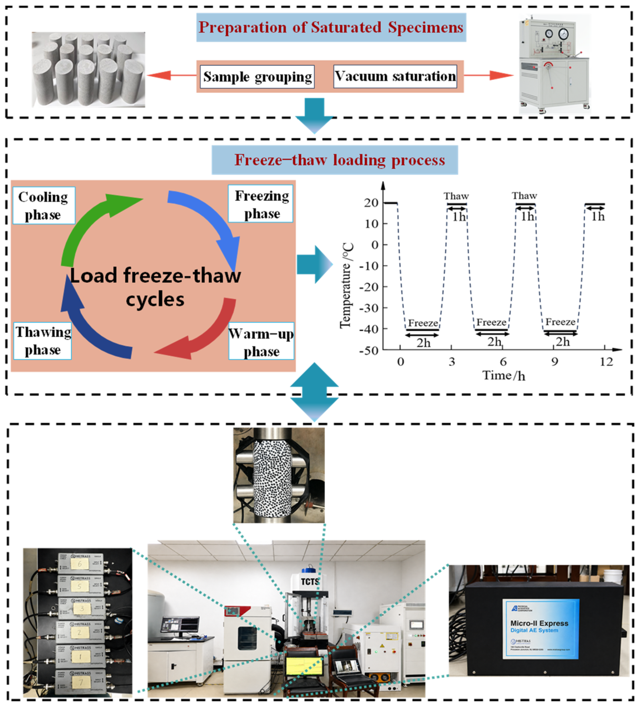
(3) Utilize the independently developed TCDR-I temperature-stress coupling testing system to conduct freeze–thaw cycles with varying temperature differentials under constant loading on the saturated specimens. The sandstone slopes in the Juhugeng mining area, located at approximately 50 m depth, with a bulk density of 26.6 kN·m⁻³, determine the loading stress at 1.4 MPa. Place the saturated specimens were placed in a small-scale high/low-temperature constant-temperature chamber for load–freeze–thaw cycling. Set the freeze–thaw temperatures according to the predefined conditions for each specimen group. After two hours of low-temperature freezing under load, maintain the specimens at ambient temperature (20 °C) for one hour, with each freeze–thaw cycle lasting three hours. Perform five freeze–thaw cycles. This setting was mainly used to control the freeze–thaw cycle number as a variable and to highlight the effect of different freeze–thaw temperature differences on the early damage response of sandstone under constant axial loading.

(4) Conduct mechanical testing on specimens subjected to freeze–thaw cycles under varying temperature differentials. After completing the predetermined number of freeze–thaw cycles, perform uniaxial compression tests using the testing system, applying uniaxial compression to rock specimens at a displacement-controlled rate of 0.02 mm/min to obtain mechanical parameters including stress–strain curves, peak strength, and elastic modulus. Concurrently, employ a sonic emission monitoring system to collect data throughout the loading process.

(5) Repeat Steps (3) and (4) were for Groups A, B, C, D, and E specimens, performing corresponding temperature differential freeze–thaw cycles, mechanical loading, and sonic emission data collection. The test procedure is depicted in Figure 3.

3. Macroscopic Mechanical Response and Energy Evolution of Loaded Saturated Sandstone Under Different Freeze–Thaw Temperature Differences

3.1. Analysis of Failure Morphological Characteristics

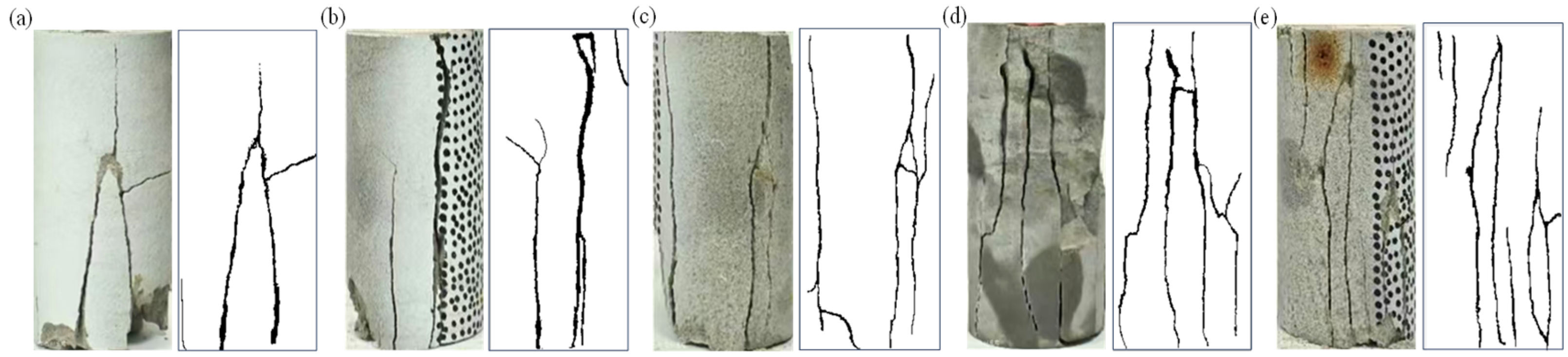
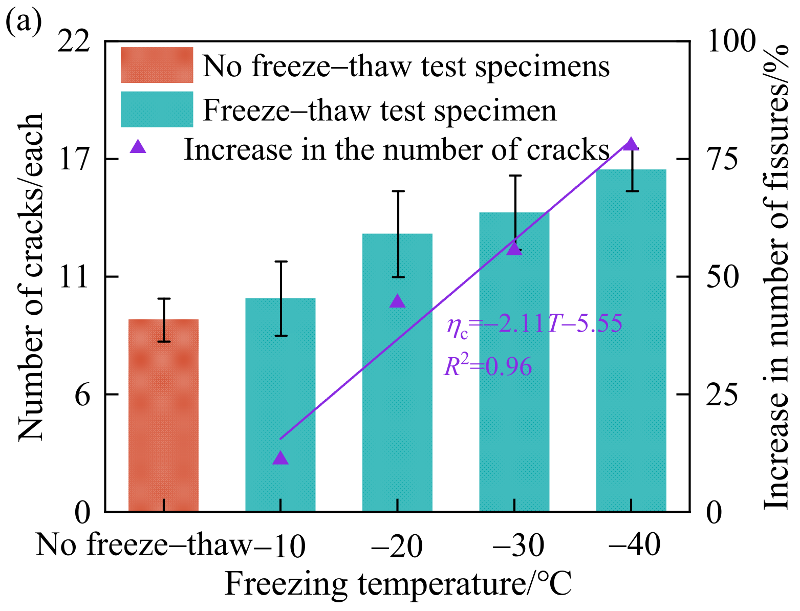
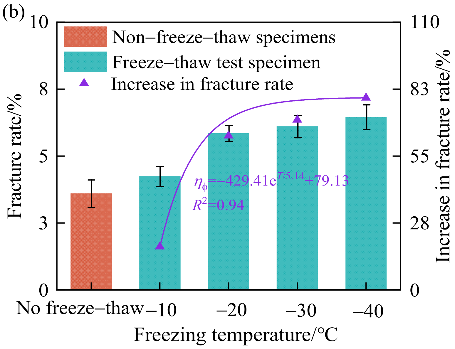
The Particles/Pores and Cracks Analysis System (PCAS) is a quantitative analysis method for pores and cracks based on digital image processing. Particles (Pores) and Cracks Analysis System (PCAS) was employed to quantitatively characterize the fracture structures in images of specimens subjected to loading until final failure under various freeze–thaw conditions. High-resolution images were binarized using a global thresholding method to distinguish fractures from the matrix; fracture segments were repaired, noise points removed, fracture networks identified, and fracture geometric parameters were output. The number of fractures and fracture density statistics were automatically calculated. The surface fracture rate is defined as the ratio of the area occupied by surface fractures to the total surface area of the specimen, with fracture structures analyzed by averaging multiple independent thresholding results [22]. The resulting fracture network images are shown in Figure 4, while Figure 5 illustrates the curves of the quantitative fracture indices of the freeze–thaw specimens as a function of the temperature differential, where T represents the freezing temperature under different freeze–thaw test conditions, with a unit of °C.

As illustrated in Figure 4 and Figure 5, the integrity of the specimens diminishes as the freeze–thaw temperature differential increases. A comparison of the fracture characteristics under various temperature ranges reveals that both the number of fractures and the fracture ratio gradually increase with the temperature differential. Specifically, under different freeze–thaw conditions, the mean number of surface fractures generated after loading was 10, 13, 14, and 16, representing relative increases of 11.11%, 44.44%, 55.55%, and 77.77%, respectively, compared to the unfrozen specimens. Meanwhile, as the freeze–thaw temperature interval expanded from −10~20 °C to −40~20 °C, the mean surface fracture ratio increased from 4.25% to 6.46%, marking increases of 17.73% and 78.95% over the unfrozen specimens. From the perspective of macroscopic failure morphology, the number of surface cracks significantly proliferated, and the failure planes gradually transitioned from a single primary crack to multiple secondary cracks. These results indicate that a larger freeze–thaw temperature differential accelerates the development of internal micro-cracks, leading to a deeper degradation of the specimen’s overall structural integrity.

3.2. Analysis of Strength and Deformation Characteristics

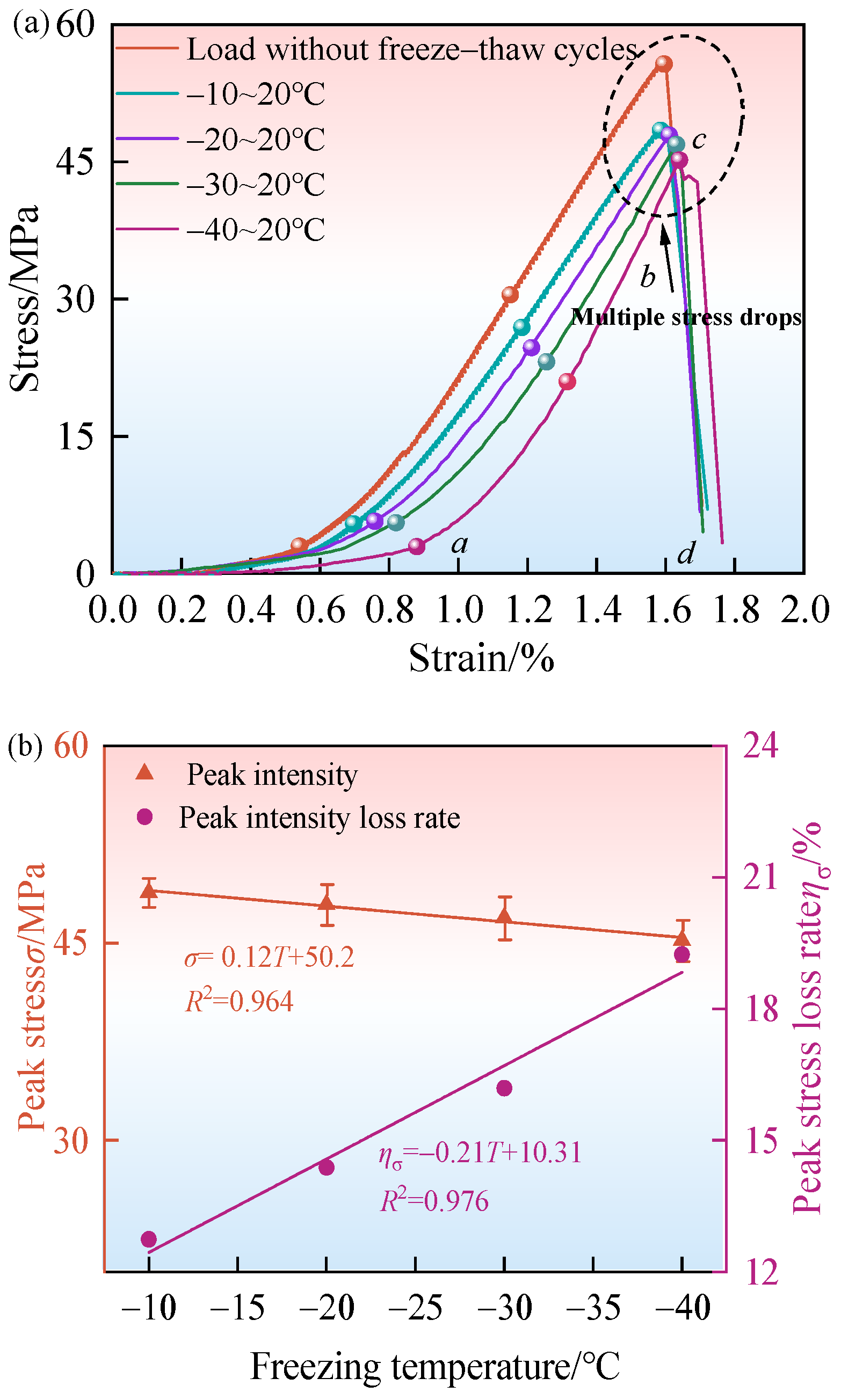
Under applied loading, the sandstone specimens exhibited freeze–thaw degradation, with their mechanical properties showing variability across freeze–thaw cycles characterized by different temperature differentials. The stress–strain curves of the sandstone under such conditions are presented in Figure 6. Further analysis identified distinct characteristics at various loading stages for specimens subjected to different freeze–thaw temperature differentials (

Table 2. Strain results from uniaxial compression tests on freeze–thawed sandstone.

Freeze–Thaw Temperature Differential/°C	Pore-Filling Compaction Section (0a)/%	Elastic Deformation Section (ab)/%	Plastic Deformation Section (bc)/%
No freeze–thaw	0~0.57	0.57~1.17	1.17~1.59
−10~20	0~0.66	0.66~1.19	1.19~1.63
−20~20	0~0.76	0.76~1.20	1.20~1.65
−30~20	0~0.81	0.81~1.22	1.22~1.69
−40~20	0~0.90	0.90~1.30	1.30~1.73

).

As indicated in Figure 6a and Table 2, the stress–strain curves for specimens under different temperature differentials can generally be divided into four stages: the pore-crack compaction stage, the elastic deformation stage, the plastic deformation stage, and the failure-instability stage [23]. The peak strength decreases as the freeze–thaw temperature differential increases, showing a negative correlation; conversely, the peak strain increases with the temperature differential, exhibiting a positive correlation. Furthermore, the 0a-compaction stage curve lengthens significantly, while the slope of the ab-elastic deformation stage curve gradually decreases and its length shortens. This indicates that following freeze–thaw cycles, internal damage structures—such as micropores and micro-cracks—continuously develop and accumulate, leading to a persistent degradation of elastic performance. In contrast, the plastic deformation capacity progressively strengthens, a trend that becomes more pronounced as the temperature differential increases. Thus, the temperature differential exerts a significant influence on the mechanical properties and damage characteristics of the specimens.

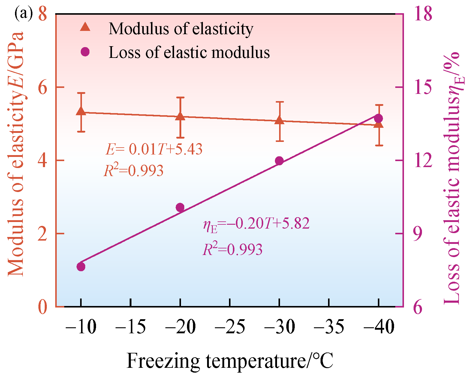
To further analyze the impact of the temperature differential on the failure characteristics of the rock specimens, three mechanical parameters, peak strength (σ), elastic modulus (E), and peak strain (ε), were fitted. The resulting variation curves for these parameters under different freeze–thaw temperature differentials are presented in Figure 6b and Figure 7.

As shown in Figure 6b, the mean peak strength gradually decreases with the increasing temperature differential, exhibiting a negative correlation; conversely, the peak strength loss rate increases with the temperature differential, showing a positive correlation. The mean peak strength of the control specimen without freeze–thaw was 55.97 MPa. After being subjected to freeze–thaw cycles at different temperature differentials, the mean peak strengths of the saturated sandstone samples were 48.84 MPa, 47.92 MPa, 46.91 MPa, and 45.20 MPa, respectively. This demonstrates a progressive attenuation of mean peak strength as the freeze–thaw temperature differential increases, with corresponding strength loss rates of 12.74%, 14.38%, 16.19%, and 19.24%. These results indicate that under the sustained action of a constant load, high-temperature-differential freeze–thaw cycles significantly intensify the microstructural degradation of the rock samples, promoting more extensive pore network reconfiguration and micro-crack expansion, which ultimately leads to a continuous decline in the overall bearing capacity of the specimens.

As illustrated in Figure 7a, the mean elastic modulus under different freeze–thaw conditions exhibits a linearly decreasing trend with the increase in temperature differential; conversely, the elastic modulus loss rate increases with the temperature differential, showing a positive correlation. When the freeze–thaw temperature ranges were −10 to 20 °C, −20 to 20 °C, −30 to 20 °C, and −40 to 20 °C, the loss rates of the mean elastic modulus compared to the unfrozen specimens were 7.64%, 10.07%, 11.98%, and 13.72%, respectively. The specimen subjected to the −40 to 20 °C temperature range exhibited the minimum elastic modulus, indicating that its capacity to resist deformation induced by external loads was significantly weakened.

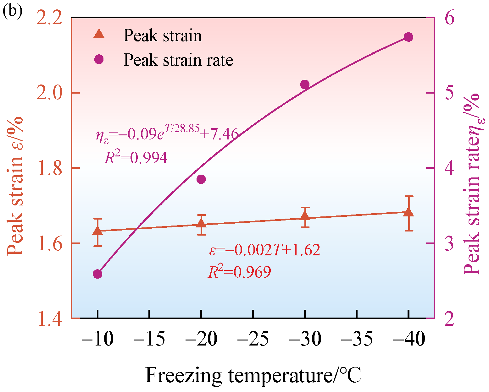
As shown in Figure 7b, the mean peak strain is positively correlated with the freeze–thaw temperature differential, gradually increasing as the differential widens. For specimens subjected to temperature ranges of −10 to 20 °C, −20 to 20 °C, −30 to 20 °C, and −40 to 20 °C, the mean peak strains under loading were 1.63%, 1.65%, 1.69%, and 1.73%, respectively. Compared to the unfrozen specimens, the variation rate of peak strain was 2.52% after freezing and thawing at a temperature differential of −10 to 20 °C; this rate increased to 8.81% when the differential reached −40 to 20 °C, which is 3.49 times that of the −10 to 20 °C condition. With the increase in the freeze–thaw temperature differential, the peak strain and its variation rate exhibit linear and non-linear growth trends, respectively. These results suggest that a higher variation rate of peak strain indicates more significant micro-crack propagation and pore structure reconfiguration within the specimens, thereby leading to a deeper degree of freeze–thaw damage.

3.3. Analysis of Energy Evolution Characteristics

The energy evolution of rock specimens during the process of damage and failure is essentially a comprehensive reflection of the coupling effect between load and strain. Compared to a simple analysis of mechanical response, an energy-based perspective provides a more intuitive revelation of the evolutionary characteristics throughout the entire process from loading to failure. The work (U) performed by external forces on the rock specimen can be regarded as the total strain energy absorbed by the specimen (kJ/m³):

$$U=U_{\mathrm{e}}+U_{\mathrm{d}}$$

(1)

Here, U_e represents the elastic strain energy during the loading and failure process of the specimen, and U_d denotes the dissipated strain energy during the same process, which is consumed by internal damage and plastic deformation within the rock.

Since this study is conducted under uniaxial compression, the total strain energy absorbed by the sandstone specimens during the loading and deformation process can be calculated using the following equation:

$$U={\displaystyle {\int }_0^{{\epsilon }_1}{\sigma }_1}\mathrm{d}\epsilon$$

(2)

$$U_{\mathrm{e}}={\displaystyle \frac{1}{2E_0}}{\sigma }_1^2$$

(3)

$$U_{\mathrm{d}}=U-U_{\mathrm{e}}$$

(4)

Here, E_i is the unloading elastic modulus of the sandstone specimen at the corresponding time, E₀ is the initial elastic modulus of the specimen, and μ is the Poisson’s ratio. In the calculation of the stored elastic strain energy, the initial elastic modulus can be used as a substitute for the unloading elastic modulus [24,25].

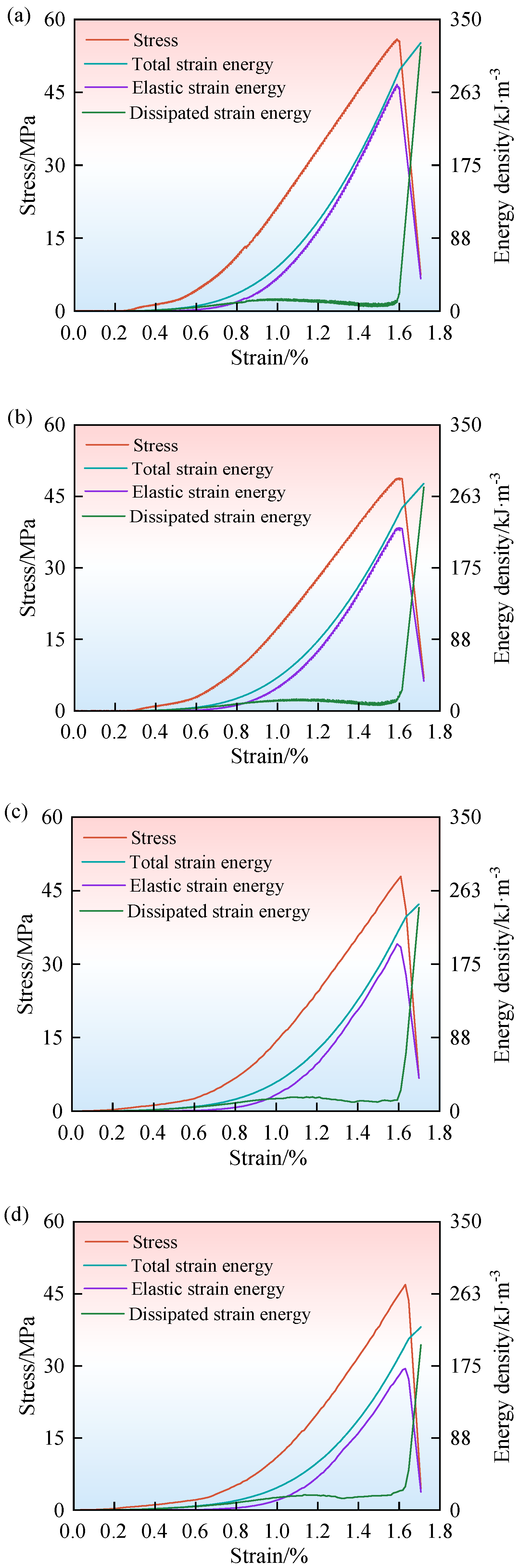
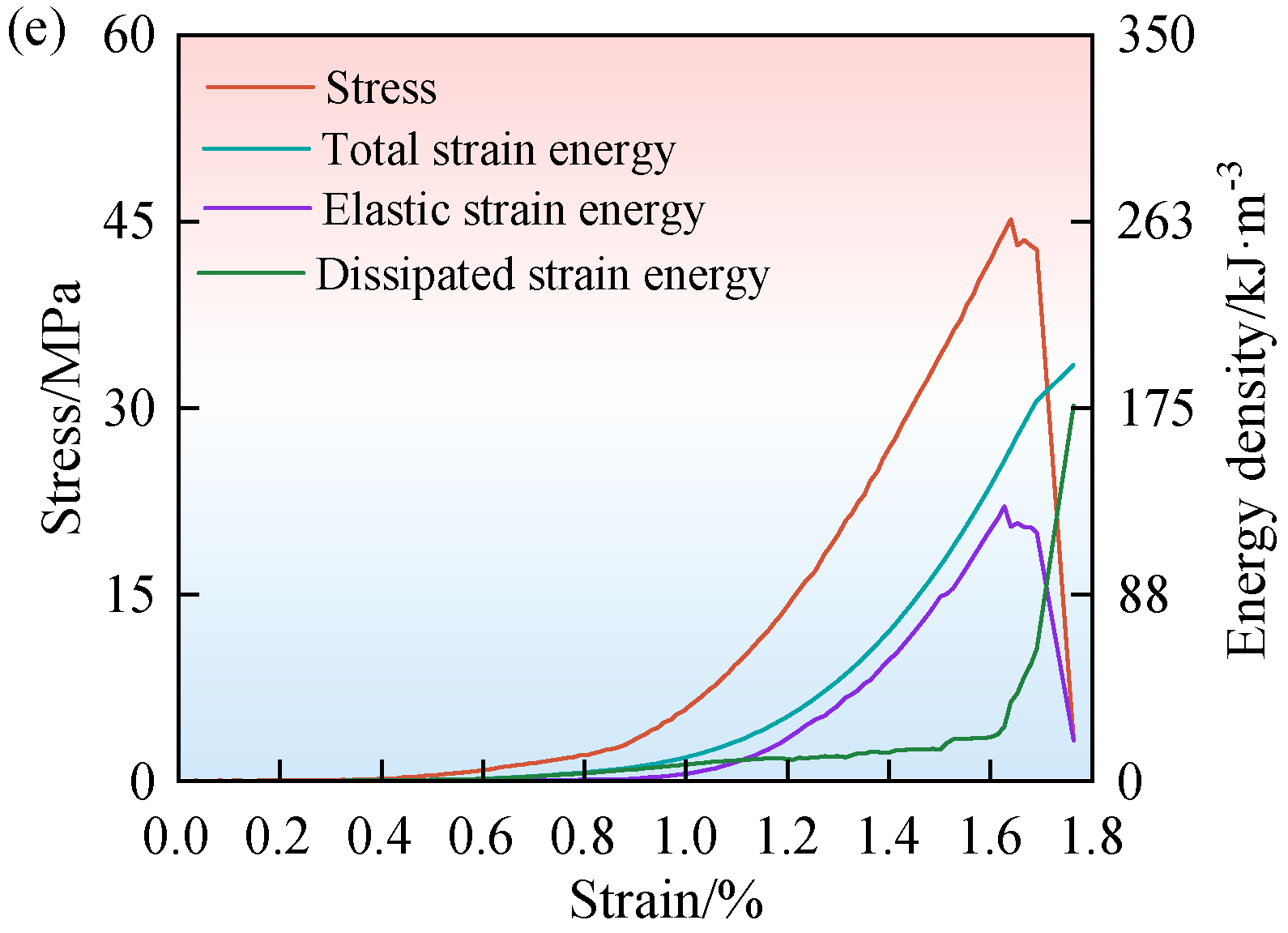
By combining Equation (1) through (4), the evolution of the total strain energy, elastic strain energy, and dissipated strain energy with respect to strain can be obtained for specimens subjected to different freeze–thaw temperature differentials under loading. The energy evolution patterns of the freeze–thawed saturated sandstone specimens are illustrated in Figure 8, and the calculation results analyzed at the peak stress point are presented in

Table 3. The results of energy calculations.

Freeze–Thaw Temperature Differential/°C	U/(kJ·m−3)	Ue/(kJ·m−3)	Ud/(kJ·m−3)
No freeze–thaw	283.86	269.31	14.55
−10~20	243.99	223.63	20.36
−20~20	219.97	195.07	24.90
−30~20	200.34	171.67	28.67
−40~20	156.77	122.31	34.46

.

As indicated by Figure 8 and Table 3, the total strain energy of the specimens accumulates continuously during the loading and failure process, exhibiting a distinct non-linear growth pattern with a characteristic concave-downward curvature in the early stages. Taking the peak stress point as the reference, it is observed that the total strain energy decreases progressively as the freeze–thaw temperature differential increases. Specifically, the total strain energy dropped from 283.86 kJ/m³ for the unfrozen specimen to 243.99, 219.97, 200.34, and 156.77 kJ/m³, representing reductions of 14.05%, 22.51%, 29.42%, and 44.77%, respectively. The evolution of elastic strain energy in the early loading stage is fundamentally consistent with that of the total strain energy; however, its growth rate gradually slows down as it approaches peak stress. Conversely, the dissipated strain energy increases with the temperature differential, rising from 14.55 kJ/m³ for the unfrozen specimen to 20.36, 24.90, 28.67, and 34.46 kJ/m³, marking increases of 39.93%, 71.13%, 97.04%, and 136.83%, respectively. It can be concluded that under constant loading, the freeze–thaw temperature differential significantly weakens the elastic strain energy storage capacity of the specimens while promoting an increase in dissipated strain energy, which further facilitates macroscopic crack initiation and strength degradation.

3.4. Analysis of Acoustic Emission Response Characteristics

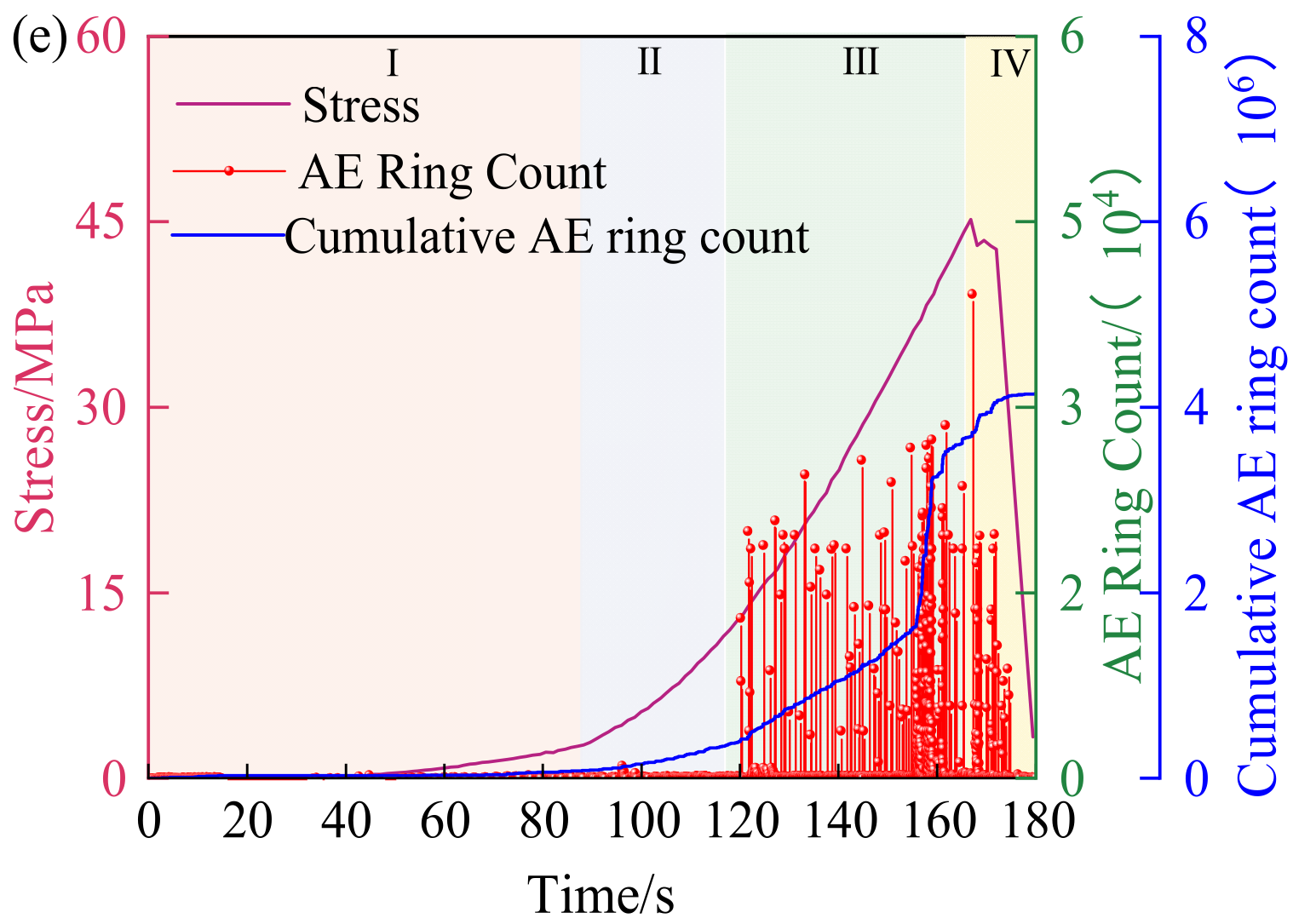
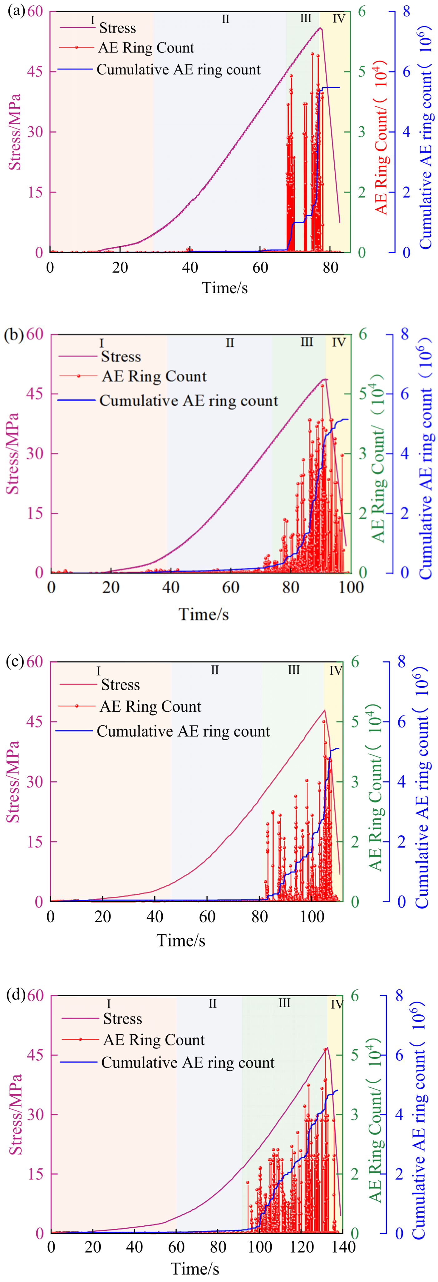
In rock mechanics testing, acoustic emission technology characterizes damage evolution and failure mechanisms by capturing transient elastic waves released during the rock fracturing process in real time [26]. Figure 9 illustrates the evolutionary characteristics of stress response, ringing counts, and cumulative ringing counts for specimens subjected to different freeze–thaw temperature differentials under constant loading. Ringing count, defined as the number of pulses where the waveform envelope of a single AE event crosses a preset threshold, serves as a fundamental parameter for characterizing AE intensity. Cumulative ringing count represents the temporal integration of all valid AE ringing counts over the entire loading history or under the influence of environmental coupling.

As illustrated in Figure 9, the entire loading process of each specimen can be divided into four distinct stages: pore-crack compaction (I), elastic deformation (II), crack propagation (III), and failure (IV). Under unfrozen or low temperature differential conditions, AE ringing counts are primarily concentrated around the peak stress point, exhibiting a pronounced pre-peak active concentration. However, as the freeze–thaw temperature differential increases, the onset of AE activity occurs progressively earlier. The distribution range of ringing counts within Stage III significantly widens, and the growth pattern of cumulative ringing counts shifts from a late-stage abrupt leap to a sustained increase over a longer duration. This indicates that the increase in temperature differential promotes the premature activation of original micro-defects and freeze–thaw-induced damage cracks, transforming the failure process from a relatively concentrated brittle instability to a progressive damage evolution.

The temporal characteristics reveal that the increase in freeze–thaw temperature differential not only alters the release mode of AE activity during loading but also weakens its overall activity capacity and release intensity. With the widening temperature differential, the gradual increase in internal pores and cracks leads to a longer duration for the pore/crack compaction stage, consequently reducing the stored and releasable elastic energy. The unfrozen specimen exhibited the maximum AE parameter values at 49,796 and 5,576,891; however, after exposure to a freeze–thaw cycle of −40 to 20 °C, these values decreased to 39,151 and 4,145,504, representing reductions of 21.38% and 25.67%, respectively. This indicates that under constant loading, both the capacity and intensity of AE activity during the loading of different specimens exhibit a downward trend. The primary reason is that the coupling of load and freeze–thaw action weakens the particle contact and cementation within the rock. The evolution of the crack network and crystal contact relationships promotes the expansion and connectivity of internal defects, thereby compromising the original structural integrity and reshaping the stress field. Ultimately, this results in a gradual reduction in the energy consumption required for dislocation, sliding, and friction between particles during the loading process.

4. Precursor Identification and Correlation Analysis of Saturated Sandstone Failure Under Pressure

4.1. Analysis of RA-AF Characteristics of Saturated Sandstone Under Coupling of Loading and Freeze–Thaw Cycles

The Rise Angle (RA)- Average Frequency(AF) ratio serves as a critical acoustic emission parameter characterizing the damage and fracture modes of specimens. The RA value is defined as the ratio of signal rise time to amplitude, where the rise time is the time interval between the trigger time and the time corresponding to the maximum amplitude, and the amplitude is the maximum amplitude of the acoustic emission waveform signal, whereas the AF value represents the ratio of ringing count to duration. The ring-down count refers to the number of oscillations exceeding the threshold during a single acoustic emission hit, while the duration is the time interval between the trigger time and the end time of the acoustic emission signal. Based on RA-AF values, damage modes within freeze–thawed rocks under varying temperature differentials can be categorized as tensile failure or shear failure. Acoustic emission fracture types are primarily classified as either tensile fracture or shear fractures [27,28]. Typically, a tensile fracture exhibits a smaller RA value and a larger AF value, while a shear fracture is characterized by a larger RA value and a smaller AF value.

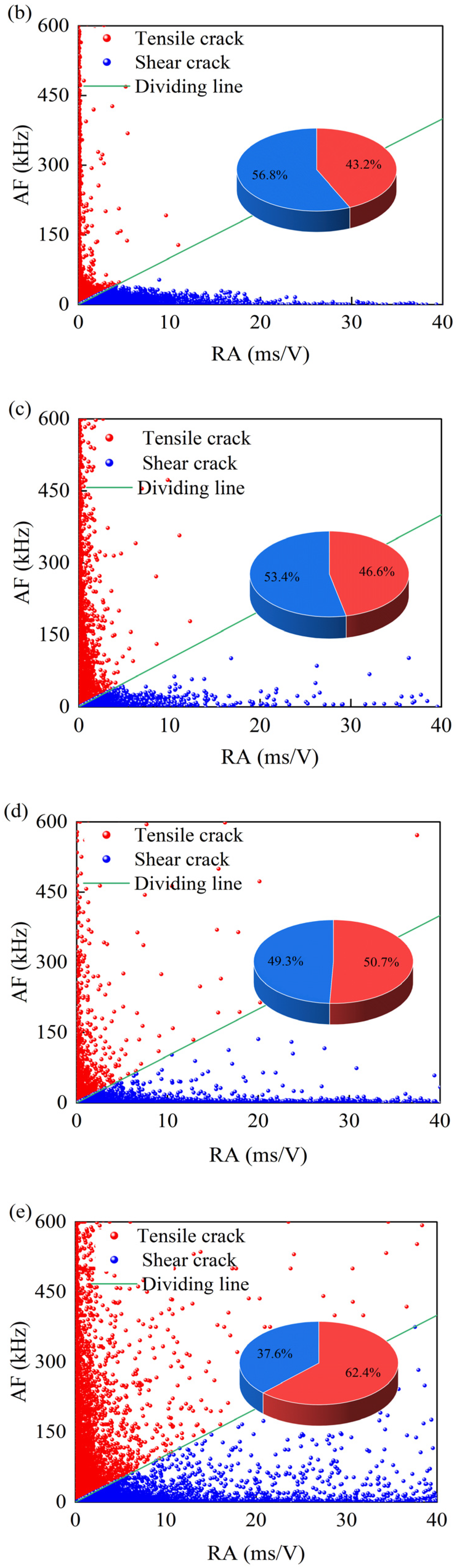
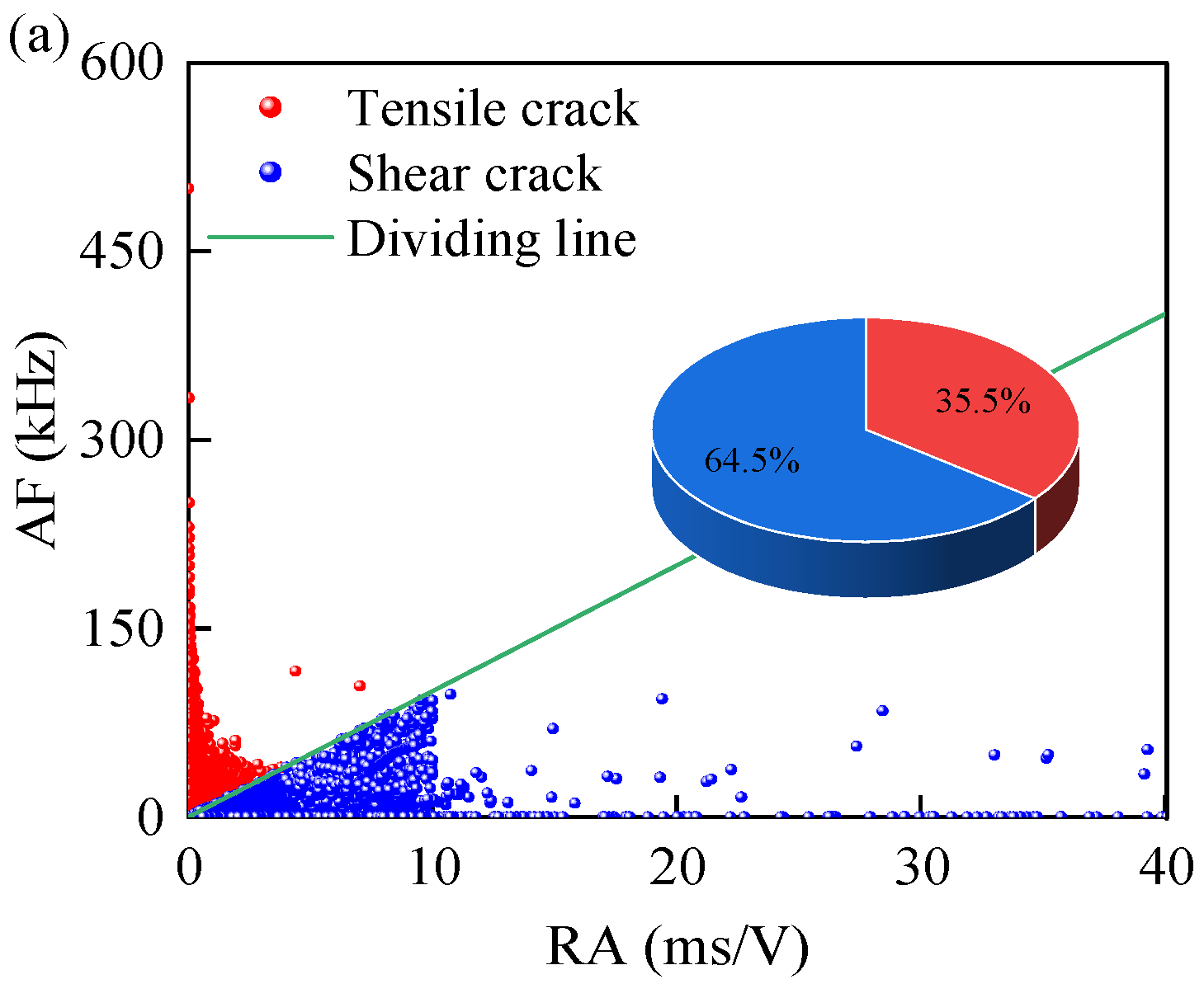
Therefore, correlation analysis of the RA-AF values can elucidate the fracture patterns of specimens during the loading of freeze–thawed sandstones subjected to different temperature differential loads. Typically, K = AF/RA is employed as the critical value to differentiate between tensile and shear cracks. Specifically, regions above the boundary line correspond to tensile-type fractures, while regions below the boundary line predominantly exhibit shear-type fractures. Building upon previous research, this study adopts K = 1 as the critical value [29] and plots the RA-AF characteristic distribution diagram to reveal the fracture characteristics of freeze–thawed rocks under different temperature differential loads during loading, as depicted in Figure 10.

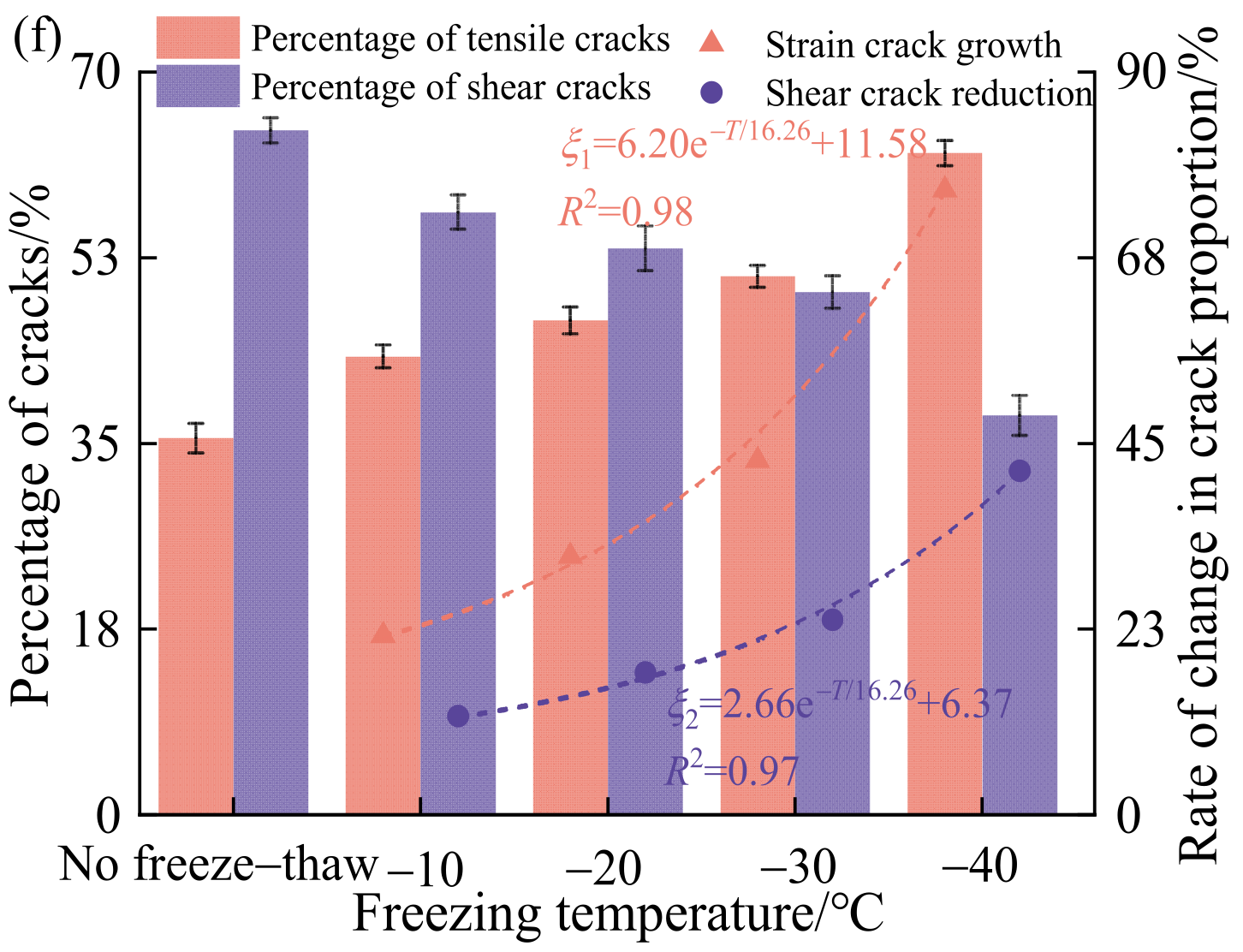
As illustrated in Figure 10, the freeze–thaw temperature gradient plays a decisive role in the evolution of the specimens’ micro-fracture mechanisms. Under unfrozen or low temperature differential conditions, although the mean percentage of tensile cracks increases steadily from 35.5% to 46.6%, the initiation and propagation of internal micro-cracks remain dominated by shear fractures, which reach a maximum percentage of 53.4%. However, after the specimens are subjected to extreme freeze–thaw temperature differentials of −30 to 20 °C and −40 to 20 °C, a dominant shift in fracture modes occurs within the specimens. The mean percentage of shear cracks drops rapidly to 37.6%, with a reduction of 41.67%, while the mean percentage of tensile cracks surges to 62.4%, gaining a clear advantage with an increase of up to 75.75%. Further data analysis reveals a highly non-linear correlation between the percentage of these two crack types and the freeze–thaw temperature differential under constant loading stress, with a goodness-of-fit R² reaching 0.97.

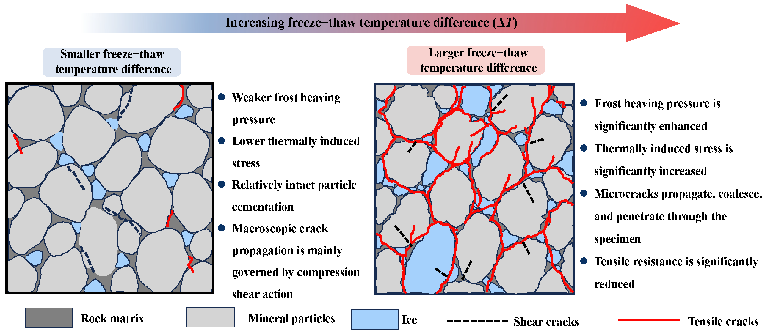
Based on the above RA-AF crack classification results, combined with the observed macroscopic failure patterns, the specimen failure mode gradually changed from shear-dominated to tensile-dominated failure with increasing freeze–thaw temperature difference. To more intuitively explain this transition process and clearly reveal the physical mechanism underlying the change in failure mode, a corresponding mechanistic schematic diagram was prepared, as shown in Figure 11.

As shown in Figure 11, with increasing freeze–thaw temperature difference(△T), the crack propagation mode of the specimens gradually shifted from shear-dominated to tensile-dominated behavior. When the freeze–thaw temperature difference was relatively small, the freezing temperature was comparatively high. As a result, the frost-heaving pressure generated by pore-water freezing was weak, the thermal stress induced by the temperature gradient was also relatively low, and the cementation between mineral particles remained relatively intact. Therefore, during the subsequent uniaxial compression loading process, crack propagation inside the specimens was mainly controlled by compression–shear action, and the failure mode exhibited a pronounced shear-dominated characteristic.

As the freeze–thaw temperature difference increased, the freezing temperature decreased, pore water froze more sufficiently, and the frost-heaving pressure increased significantly. Meanwhile, the mismatch in thermal expansion and contraction among mineral particles, pore ice, and the rock matrix became more pronounced, resulting in a substantial increase in thermally induced stress and more obvious stress concentration around pre-existing pores, micro-cracks, and weakly cemented interfaces. Previous studies [30,31] have indicated that freeze–thaw action can be approximately regarded as a low-cycle fatigue loading process. At the microscopic scale, the expansion pressure generated by pore-water freezing induces tensile stress on pore walls and pre-existingmicro-crackss. At the macroscopic scale, this effect is equivalent to tensile loading acting on the rock specimen. Therefore, a larger freeze–thaw temperature difference promotes the opening, propagation, coalescence, and penetration of pre-existing pores andmicro-crackss, thereby markedly reducing the tensile resistance of the specimen.

In addition, after freeze–thaw treatment, micro-cracks inside the specimens gradually connect with each other, and the specimens often exhibit multi-section tensile failure at the macroscopic scale. As the intensity of freeze–thaw temperature action increases, the number of macroscopic fracture surfaces increases, and longitudinal penetrating cracks become more evident [32]. This is in good agreement with the RA-AF crack-type evolution and the observed macroscopic failure patterns in this study. These results indicate that an increase in freeze–thaw temperature difference not only intensifies the internal damage of the specimens, but also changes the dominant mechanism of crack initiation and propagation. Specifically, the failure mode gradually shifts from compression-shear control under smaller freeze–thaw temperature differences to tensile cracking control under larger freeze–thaw temperature differences.

4.2. Evolutionary Characteristics of Acoustic Emission b-Value During the Failure Process

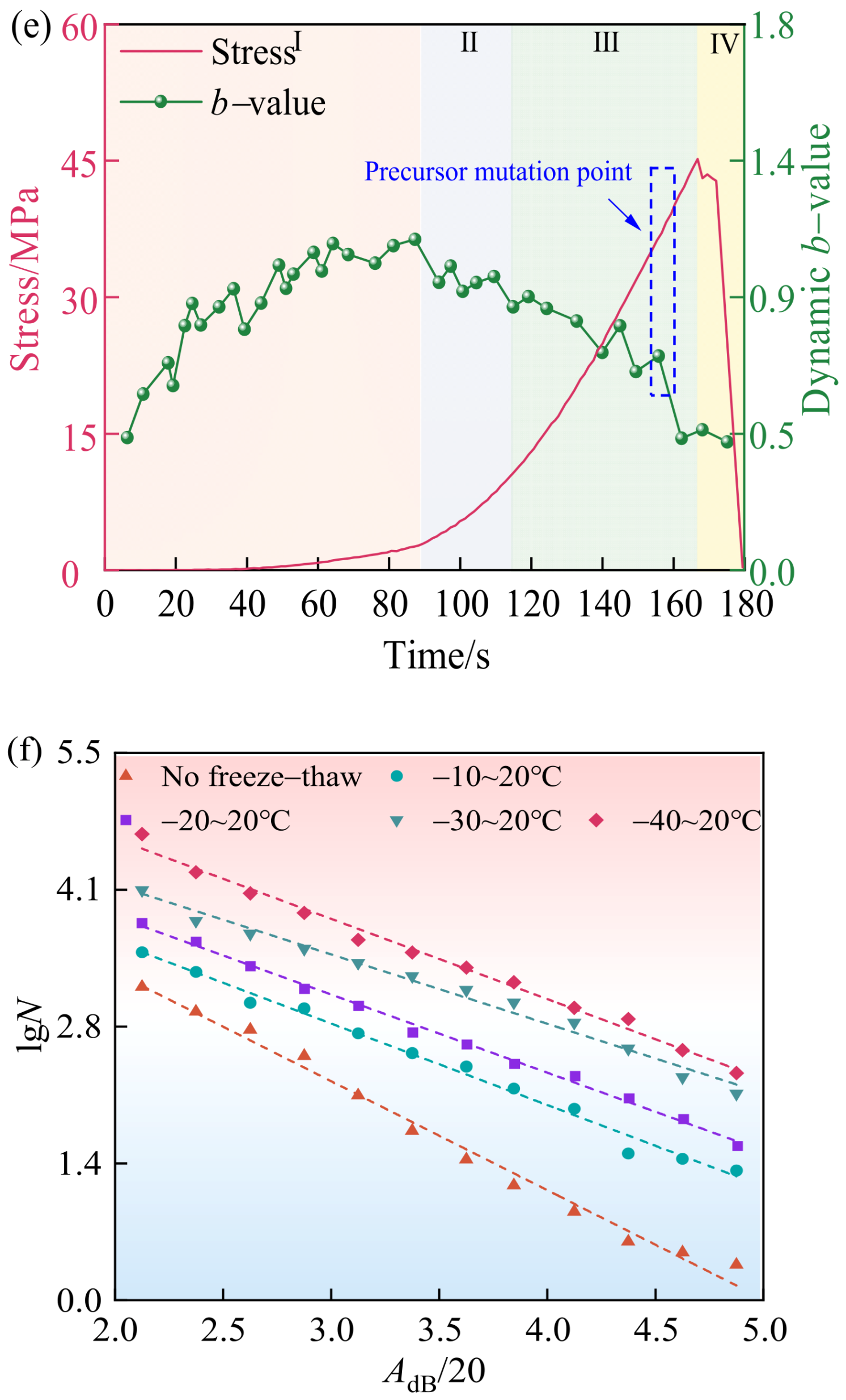
The evolution of the b-value over time reflects the underlying patterns of average strength, stress states, and micro-crack scales within the rock [33]. It is widely recognized as a precursor to coal and rock mass failure, serving as a standard for evaluating the distribution of small-scale versus large-scale micro-fracture events within the specimen.

In seismology, the b-value characterizes the relationship between earthquake magnitude and frequency, as delineated by the Gutenberg–Richter law (G-R law) [34]. This relationship is expressed in Equation (5):

$$logN\left(M\right)=a-bM$$

(5)

Here, N represents the number of seismic events within the magnitude range from M to M + ΔM; M denotes the magnitude; a is the fitting constant; and the magnitude M can be converted from amplitude, M = A/20A_dB, where A_dB is the acoustic emission amplitude in decibels (dB).

The value of b is further calculated using the maximum likelihood method [35], which is formulated into Equation (6):

$$b={\displaystyle \frac{{\log }_{10}\mathrm{e}}{\overline{M}-M_{\min }}}$$

(6)

Here, $\overline{M}$ represents the average magnitude; M_min denotes the minimum magnitude; e is the natural constant; and where e is Euler’s number, furthermore, log e = 0.4343.

Drawing on the b-value theory from seismology, the dynamic b-values during the loading process were calculated using Equations (5) and (6) to reveal the evolution of internal damage and failure. In the data processing, a sliding window algorithm was employed to group acoustic emission events chronologically. Each calculation window consisted of 200 events with a sliding step of 50 events, and the magnitude interval was set to 5 dB. 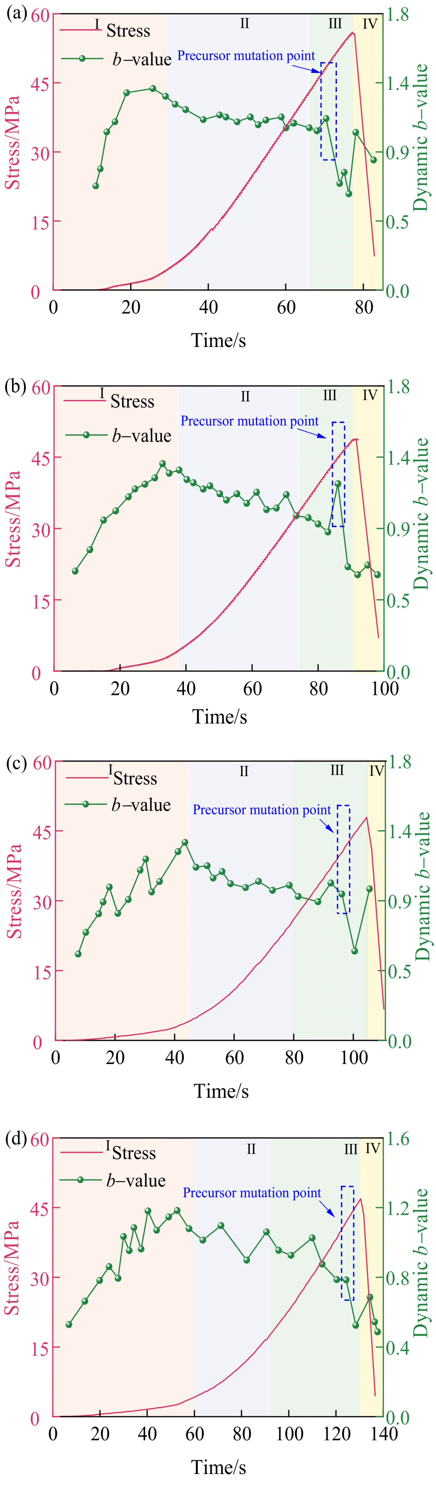The calculated b-value was assigned to the timestamp at the end of each window, from which the dynamic b-value evolution curves over time were plotted, as shown in Figure 12.

The dynamic b-value during the loading process effectively characterizes the energy distribution and damage progression of the specimen’s fracturing. An increase in the b-value indicates that AE activity is dominated by low-magnitude events, suggesting that the rock is primarily undergoing the initiation and propagation of micro-cracks. In this stage, crack development is relatively dispersed, the propagation rate is slow, and the damage evolution is comparatively mild. Conversely, a decrease in the b-value signifies an increasing proportion of high-magnitude events, indicating the coalescence and failure of larger-scale fractures within the rock, accompanied by a significantly accelerated crack propagation rate and concentrated energy release. Therefore, the magnitude of change in the b-value serves as a critical indicator for measuring the severity of rock damage and its stage of failure evolution.

As shown in Figure 12, the b-value exhibits distinct periodic fluctuations throughout the loading process, characterized by an initial increase followed by a subsequent decrease. During the pore-crack compaction stage (I), the b-value rises gradually, indicating the initiation and propagation of micro-cracks and an increase in small-scale fracturing events. In the elastic stage (II), the b-value fluctuates within a certain threshold range; during this stage, crack activity displays multi-scale characteristics, with large and small cracks propagating alternately and competing with one another. In the plastic stage (III), the AE b-value decreases progressively while the AE hit density and activity level increase significantly. This suggests that internal cracks are propagating at an accelerated rate and coalescing, leading to severe degradation of the rock’s internal structure.

An analysis of the initial rising stage of the acoustic emission b-value reveals that the starting point and maximum b-value of the specimens gradually decrease following exposure to different freeze–thaw temperature differentials, accompanied by a significant increase in curve fluctuations. This suggests that the freeze–thaw action leads to the generation of multi-scale initial defects and enhanced heterogeneity, such that the mechanical response in this stage is no longer dominated by a single micro-crack closure mechanism. Furthermore, after freeze–thaw cycles, the decline phase of the b-value occurs at 91.86% (−10 to 20 °C), 84.72% (−20 to 20 °C), 82.87% (−30 to 20 °C), and 80.10% (−40 to 20 °C) of the loading process, representing an advancement of 0.28%, 7.42%, 9.27%, and 12.01%, respectively, compared to the pre-freeze–thaw state. This indicates that micro-cracks generated by freeze–thaw cycles tend to coalesce more easily during loading, accelerating crack propagation and causing the specimens to enter the dynamic b-value decline phase at lower stress levels. These findings are consistent with the previously discussed evolution of cumulative ringing counts and align with the research results reported by Zhang Huimei et al. [36].

To further investigate the overall distribution characteristics, the b-value was comprehensively calculated using Equation (5). The average b-value for the unfrozen sandstone was 1.163. As the freeze–thaw temperature differential increased to −10 to 20 °C, −20 to 20 °C, and −30 to 20 °C, the b-values dropped to 0.7791, 0.7539, and 0.7369, respectively. This indicates that with the increase in temperature differential, the proportion of micro-cracks within the rock mass gradually decreases, and large-scale structural fractures become dominant. However, when the temperature differential further increased to −40 to 20 °C, the b-value rebounded to 1.1241. This suggests that the internal structure of the sandstone specimen is fully degraded; the uneven development of internal defects leads to a reduction in large-scale failure events, replaced by the extensive convergence and coalescence of micro-cracks.

Overall, the b-value of the sandstone exhibits a downward trend as the freeze–thaw temperature differential increases. This characteristic reflects the evolutionary process of the rock mass from a uniform damage stage dominated by micro-cracks to a heterogeneous degraded stage dominated by large-scale fractures. Freeze–thaw action weakens the overall bearing skeleton of the rock mass, shifting the energy release mode from concentrated and sudden to dispersed and gradual. Simultaneously, the relative activity of small-scale cracks decreases while the proportion of high-energy events increases, ultimately leading to the overall decline in the b-value.

4.3. Critical Slowing Down Theory and Multi-Parameter Acoustic Emission Precursor Identification

In the evolutionary process of a dynamic system, the critical phase where the system transitions from its original steady state to a new one is often accompanied by characteristic phenomena such as a significant increase in response amplitude, a reduction in the decay rate of disturbances, and an extension of recovery time [37,38]. These features reflect a trend of heightened sensitivity to external disturbances and diminished stability, a phenomenon known as critical slowing down. As a concept in statistical physics, the theory of critical slowing down is typically employed to describe the distribution and fluctuation phenomena that occur when a complex dynamic system undergoes a critical transition upon reaching a tipping point.

In statistics, the variance V² is used to characterize the degree of deviation of sample data from the mean, and it can be calculated using the following equation:

$$V^2={\displaystyle \frac{1}{n}}{{\displaystyle \sum _{i=1}^n\left(h_i-\overline{h}\right)}}^2$$

(7)

Here, V² denotes the variance, which is dimensionless; n represents the number of data points; h_i denotes the i-th data point of the characteristic signal quantity in the acoustic emission system; $\stackrel{—}{h}$ denotes the mean value of the acoustic emission characteristic parameter.

Assuming the existence of a forced disturbance with a period of Δt within the state variables, where the return to equilibrium approximates exponential regression and the recovery rate during the disturbance follows an exponential process with a rate of γ, the Autoregressive AR(1) denotes a first-order autoregressive model, in which the state of the system at the next time step is mainly determined by its state at the previous time step and a stochastic disturbance. The “1” indicates that the model only considers the influence of the immediately preceding state on the current state. Its expression is given as follows:

$$y_{\mathrm{n}+1}={\mathrm{e}}^{\gamma △t}{y}_{\mathrm{n}}+s{\beta }_{\mathrm{n}}$$

(8)

Here, y_n denotes the deviation of the system variable from equilibrium; β_n represents a normally distributed random variable.

Through the analysis of variance with AR(1), Equation (9) is derived:

$$Var(y_{\mathrm{n}+1})=M({y^2}_{\mathrm{n}})+{\left[M\left(y_{\mathrm{n}}\right)\right]}^2={\displaystyle \frac{V^2}{1-a^2}}$$

(9)

Here, Var(y_n+1) denotes the variance of the model.

As the system approaches a critical state, the internal feedback mechanisms within the specimen tend to weaken, leading to a significant delay in the system’s recovery from micro-disturbances. The correlation between adjacent states in the time series continuously strengthens, while the recovery speed of the system tends toward zero, exhibiting a classic critical slowing down phenomenon. Consequently, a sustained increase in variance is regarded as a precursor signal of system instability.

Analytical results based on the theory of critical slowing down indicate that while the selection of window length and lag step may affect the absolute magnitude of variance to some extent, the identified precursor locations and overall evolutionary trends remain fundamentally consistent. 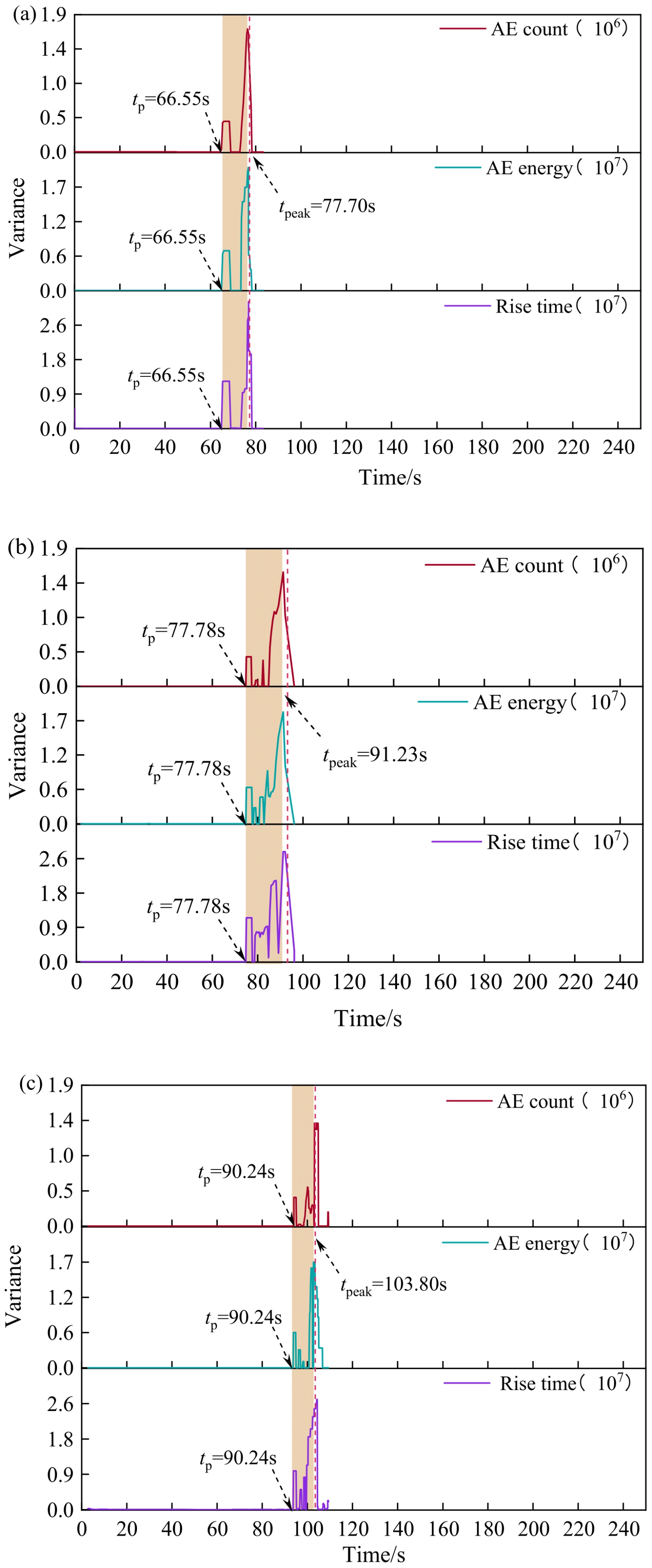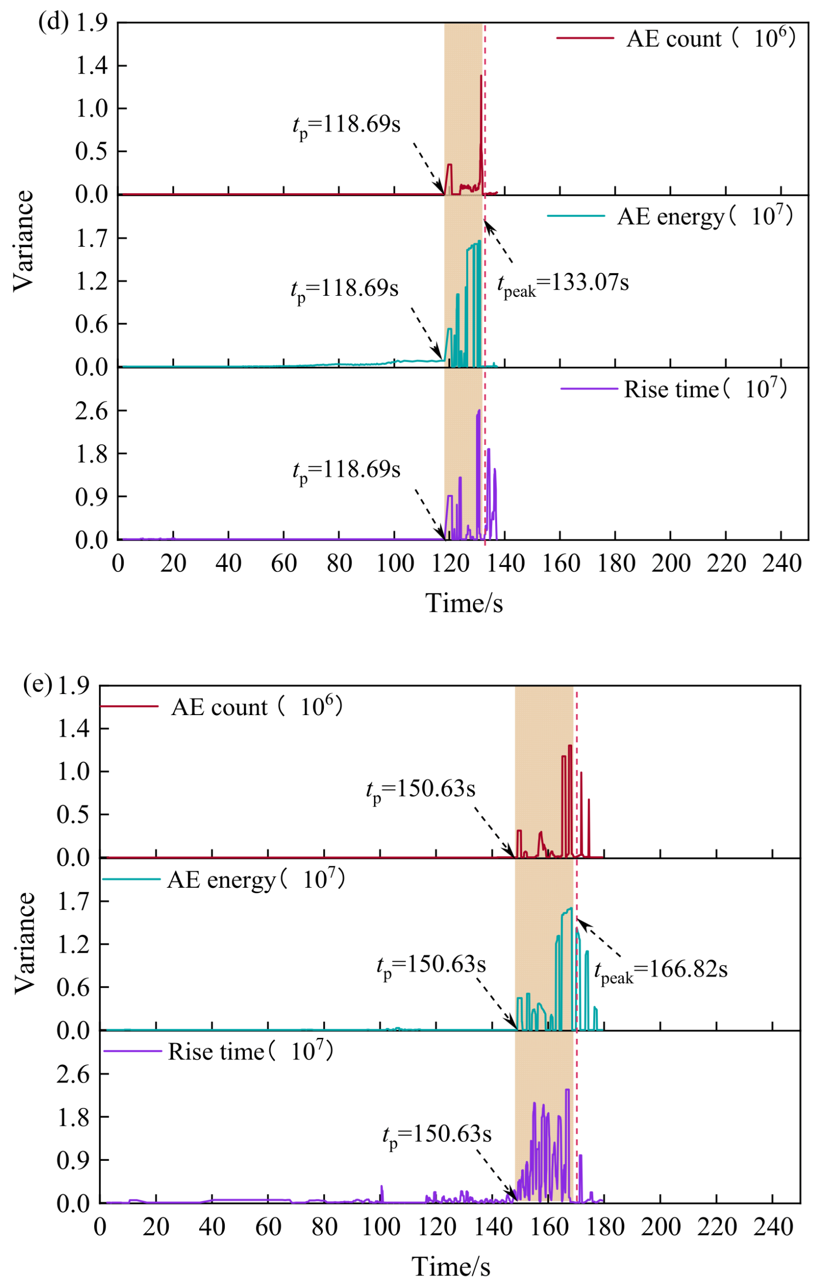This suggests that the influence of window length and lag step on precursory information can be neglected [39,40]. To ensure effective identification of precursory features while balancing AE sampling frequency and data volume requirements, this study adopts a window length of 200 and a lag step of 200. A systematic analysis was conducted on the variance of ringing counts, energy, and rise time for rock specimens under various freeze–thaw temperature differentials. This analysis aims to explore the precursory response patterns during the transition from cumulative damage to macroscopic instability. The variation curves of AE parameter variances under different freeze–thaw temperature differentials are illustrated in Figure 13.

An analysis of Figure 13a–e reveals that following freeze–thaw treatment at various temperature differentials, the internal structure of the specimens remains relatively intact and stable during the compaction and elastic stages. At this point, significant micro-crack initiation has not yet occurred, resulting in weak acoustic emission signal intensity and fewer captured acoustic emission events; consequently, the variances of acoustic emission parameters fluctuate stably within a narrow range. As loading progresses into the elastic stage and the early yield stage, micro-cracks gradually initiate and coalesce, leading to a progressive increase in the fluctuation amplitude of the variances for ringing counts, energy, and rise time. From the plastic stage to the crack failure stage, the system approaches instability, its recovery capacity diminishes, and internal disturbances within the specimen fail to decay rapidly, resulting in stochastic oscillations. As the specimen nears failure, the rate of crack propagation accelerates, acoustic emission activity surges, and parameter values increase significantly again at the peak. Overall, the abrupt rise in these three acoustic emission parameters following an initial period of steady variation can serve as a precursor point for failure.

In addition, an integrated analysis of the evolution of the acoustic emission parameter variance curves in Figure 13 was conducted. Overall, the variance evolution characteristics of the three acoustic emission parameters are similar, featuring a transition from a steady state to a sudden surge as the failure precursor point is approached. Notably, the fluctuation amplitude of the acoustic emission rise time variance is significantly larger than those of the other two parameters.

Figure 13 details the acoustic emission parameters of ringing counts, energy, and rise times for load–freeze–thaw specimens under various conditions: no freeze–thaw, −10 °C to 20 °C, −20 °C to 20 °C, −30 °C to 20 °C, and −40 °C to 20 °C. In these tests, the initial onset jump times relative to specimen failure under the conditions of no freeze–thaw, −10 °C to 20 °C, −20 °C to 20 °C, −30 °C to 20 °C, and −40 °C to 20 °C were 11.15, 13.45, 13.56, 16.19 s, respectively. Upon loading to failure, the variance of acoustic emission parameters began to fluctuate upwards. Under the aforementioned conditions, the first onset jump times were 66.55, 77.78, 90.24, 118.69, 150.63 s, respectively.

4.4. Correlation Analysis Between Crack Evolution and Acoustic Emission Precursory Response

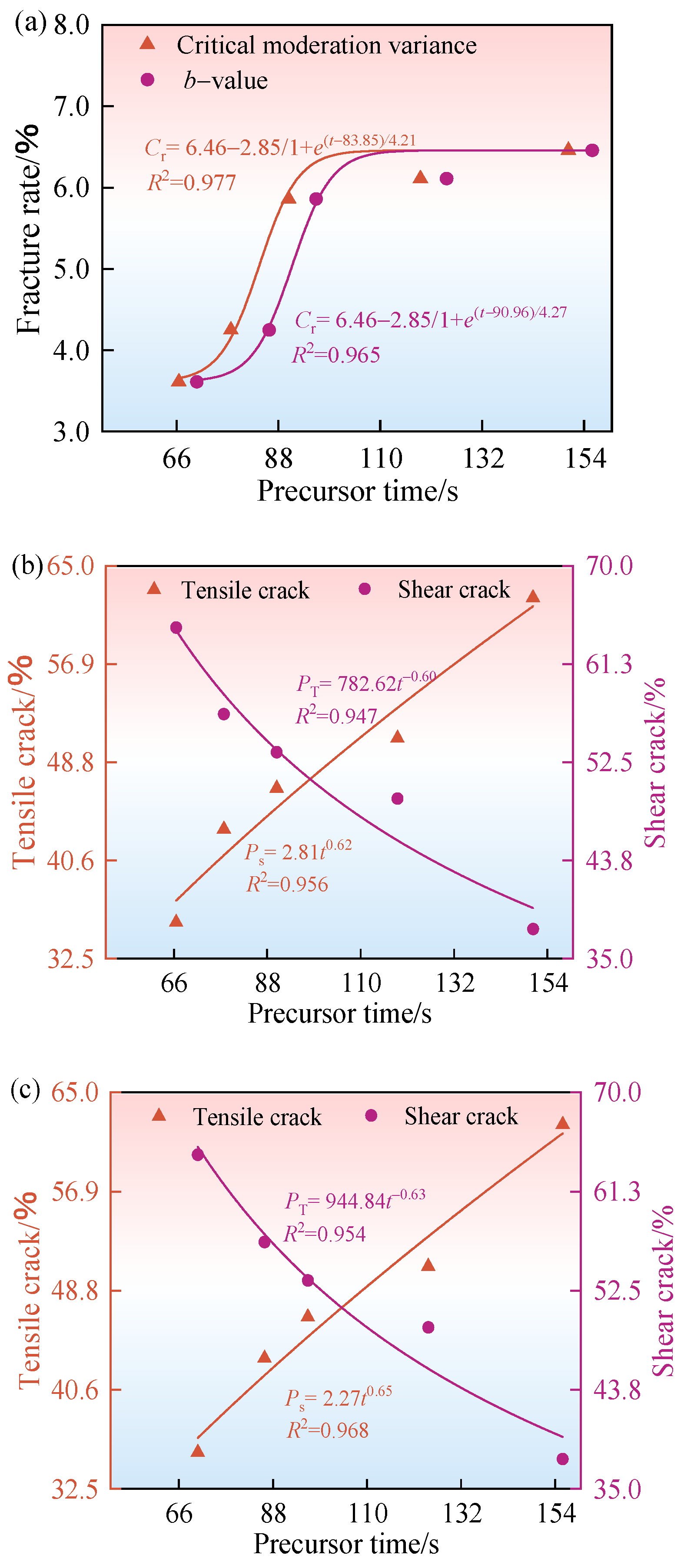
The precursory time of specimen failure is closely related to crack evolution, and together they characterize the damage accumulation and instability process of saturated sandstone under pressure following freeze–thaw treatment. To reveal the relationship between these two factors, this study selects fracture porosity, the proportion of tensile cracks, and the proportion of shear cracks as damage characterization indicators, and performs a fitting analysis against the precursory times identified by various parameters. The results are presented in Figure 14.

According to Figure 14a, the surface fracture porosity of the specimens exhibits an exponential growth trend as the precursory time increases. For instance, when the precursory time of the critical slowing down variance increased from 66.55 s to 150.63 s, the surface fracture porosity increased by 78.95%. Simultaneously, as shown in Figure 14b,c, a strong correlation exists between the precursory times of critical slowing down and b-values and the proportions of tensile and shear cracks. With the extension of the precursory time, the proportion of tensile cracks increases exponentially, whereas the proportion of shear cracks decreases exponentially.

A comprehensive analysis reveals a significant correlation between the internal failure precursory time and the crack evolution characteristics. A longer precursory time is associated with a marked increase in surface fracture porosity, indicating that as freeze–thaw damage intensifies, the rock undergoes a more thorough process of crack initiation and propagation during the pre-instability stage. Thus, the precursory time effectively characterizes the degree of fracture development and the level of damage accumulation under freeze–thaw action. Furthermore, the increasing proportion of tensile cracks alongside the decreasing proportion of shear cracks reflects an evolutionary shift in the rock failure mechanism from shear-dominated to tensile-dominated. Freeze–thaw action further facilitates the transition of internal stress concentration from localized structural plane sliding to tensile expansion at crack tips, thereby altering the crack propagation paths and the dominant failure modes. This demonstrates that the precursory time can effectively characterize the cumulative degree of freeze–thaw damage and the critical state of failure.

5. Discussion

The aforementioned research demonstrates that the synergistic effect of constant loading and freeze–thaw temperature differentials exerts a significant influence on the mechanical properties, damage evolution, and failure precursors of the specimens. As the temperature differential increases, the primary pores and micro-cracks within the specimen continuously propagate and coalesce under the constraints of repeated freeze–thaw cycles and sustained constant loading. Macroscopically, this is manifested as a reduction in peak strength, a decrease in the elastic modulus, shifts in peak strain, and a continuous increase in both crack quantity and fracture porosity. Correspondingly, the internal energy distribution of the specimens undergoes a distinct adjustment, characterized by a weakened storage capacity for elastic strain energy and an increasing trend in dissipated strain energy. This indicates the continuous accumulation of internal damage and the progressive weakening of structural stability. As internal damage accumulates and approaches a critical state, the crack propagation mode transitions from the early, relatively dispersed and stable initiation of micro-cracks to more active, large-scale crack propagation and coalescence in the later stages. Consequently, as the specimen nears instability, the acoustic emission parameters, b-values, and critical slowing down indicators typically exhibit anomalous responses, forming identifiable precursory information.

The fundamental reason for the aforementioned phenomena lies in the fact that the ice–water phase transition process of pore water during freeze–thaw cycles exhibits a strong size effect, which is further amplified by the heterogeneity of localized damage evolution under constant loading [41,42]. The internal pore size distribution of rock is complex, and the freezing temperatures of pore water vary across different scales of pores. According to the relationship between the freezing temperature of pore water and pore diameter, smaller pores correspond to lower freezing temperatures. Consequently, under the same freeze–thaw temperature differential, the water in all pores does not freeze simultaneously. Instead, water in larger connected pores and primary channels freezes preferentially, whereas freezing is delayed in micro-pores, isolated closed pores, and dead-end pores some of which may even remain unfrozen within a certain temperature range. The calculation for the relationship between pore diameter and temperature is presented in Equation (10) [43].

$$T_f=-{\displaystyle \frac{v_s{T}_A}{L}}{\displaystyle \frac{2{\gamma }_{\mathrm{SL}}}{R}}$$

(10)

Here, T_f is the freezing temperature of the pore free unfrozen water, °C; γ_SL is the ice-water interfacial tension, taken as 29 mN/m; v_s is the specific volume of ice, m³/kg; L is the latent heat of fusion for pure water, taken as 3.34 × 10⁹ cm²/s²; T_A is the absolute freezing temperature of pure water, taken as 273.15 K; and R is the effective radius of the pore, μm.

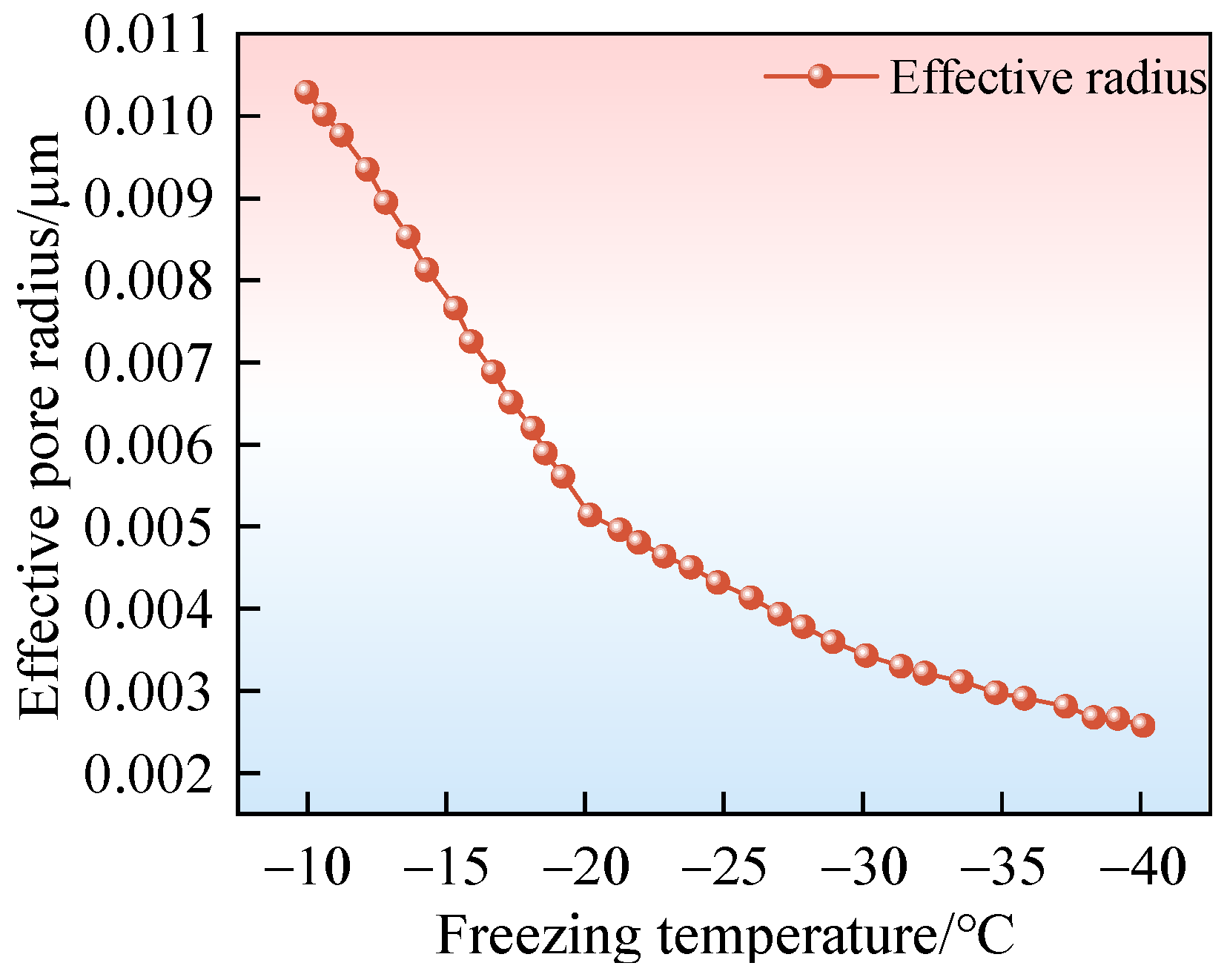
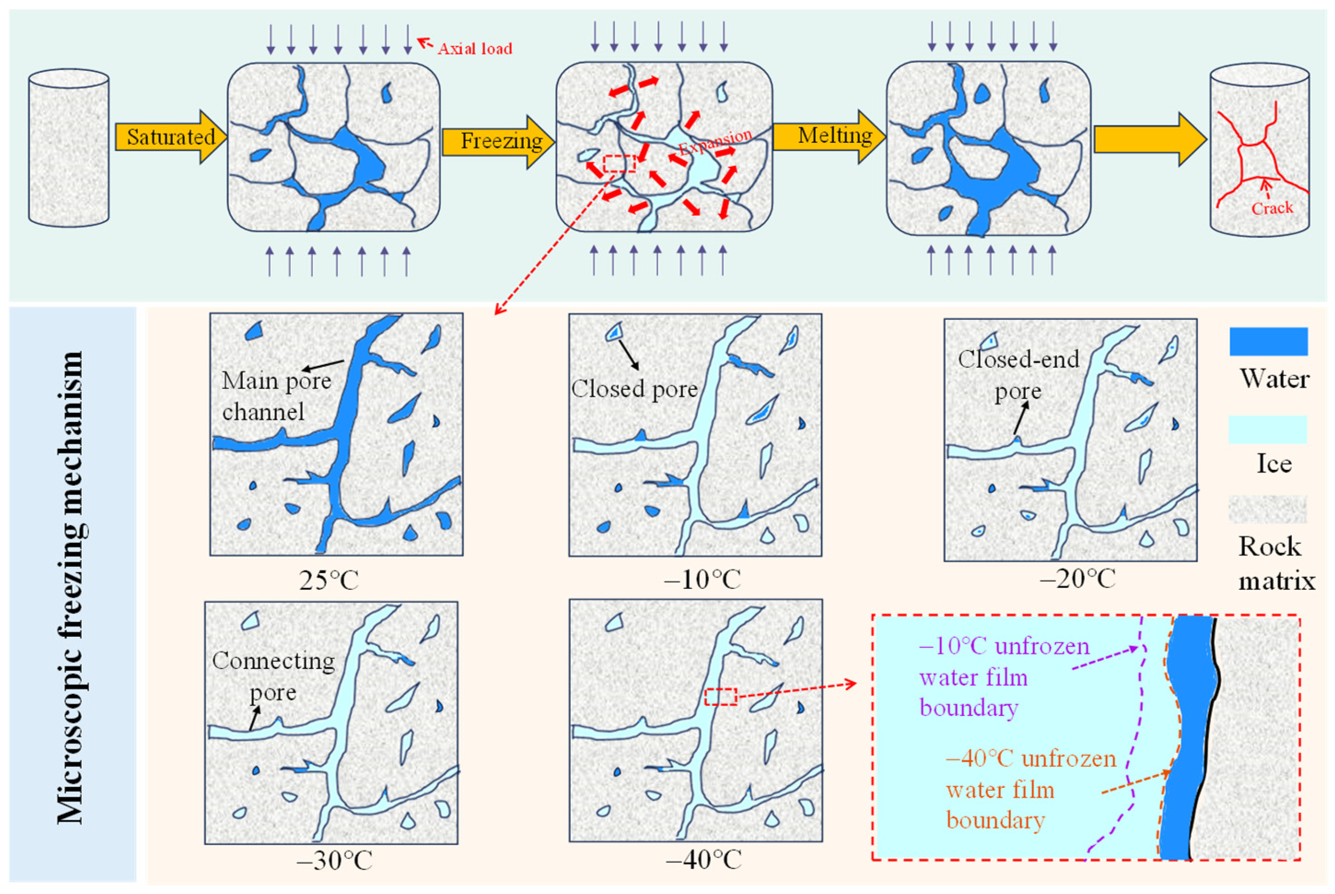
The relationship between the effective radius of internal pores and the freezing temperature was calculated according to Equation (10), as illustrated in Figure 15. The figure indicates that as the freezing temperature continues to decrease, the range of pores involved in the freezing process within the specimen gradually expands. The phase transition of pore water develops from a localized occurrence into a broader range. This asynchrony in pore freezing is one of the critical reasons for the subsequent evolution of internal damage and the differences in macroscopic response. As summarized in Figure 16 which outlines the general characteristics of the freezing process at the pore scale, water in larger connected pores freezes preferentially when the freezing temperature drops from −10 °C to −40 °C, while water in some micro-pores remains in a partially unfrozen state.

In addition, the presence of an unfrozen water film near the pore walls during the freezing process is a critical factor influencing damage evolution. This unfrozen water is maintained by the combined effects of pore wall adsorption and interfacial phenomena; its thickness is controlled by temperature and gradually decreases as the temperature drops. The existence of this unfrozen water film ensures that the contact between ice crystals, liquid water, and the rock skeleton is not purely rigid, forming instead an interfacial layer that provides a degree of buffering and transition. As the temperature continues to decrease, this interfacial layer thins, leading to a progressive weakening of the local deformation coordination and stress-release capacity. Consequently, the direct interaction between the ice phase and the rock matrix intensifies, allowing the localized pressure generated by frost heave to be more readily transmitted into the skeleton. Based on phase equilibrium theory, Döppenschmidt et al. [44,45] derived a formula for the thickness of the unfrozen water film in frozen pores as a function of freezing temperature. This formula further calculates the thickness of non-free unfrozen water films in frozen pores, as presented in Equations (11) and (12), explaining the relationship between unfrozen water film thickness and temperature.

$$d=\left(-{\displaystyle \frac{2{\sigma }^2\Delta \gamma T_{\mathrm{m}}}{{\rho }_{w}l\Delta T}}\right)$$

(11)

where

$$\Delta \gamma ={\gamma }_{iw}+{\gamma }_{ws}-{\gamma }_{is}$$

(12)

Here, d is the thickness of the non-free unfrozen water film, nm; γ_iw, γ_ws, and γ_is are the ice-water interfacial free energy, the water-rock interfacial free energy, and the ice-rock interfacial free energy, respectively, kg/s²; ρ_w is the density of bulk water, kg/m³; l is the latent heat of the ice–water phase transition, m²/s²; T_m is the freezing point of bulk water under normal pressure, which is 273.15 K at standard atmospheric pressure; and σ is the atomic spacing, nm.

Under the constant axial load, the boundaries of pre-existing pores, micro-crack tips, and weakly cemented interfaces inside the specimen remain in a sustained stress state. It should be noted that the constant load level applied in this study is relatively low and is not considered the primary factor independently governing specimen damage deterioration. Instead, it serves as a stress boundary condition during freeze–thaw cycling and participates in the damage evolution process. As the freeze–thaw temperature difference increases, more pore water participates in freezing, and ice-phase expansion induces stronger frost-heaving pressure within the confined pore space. This pressure acts together with the external constant load, making stress concentration around pore boundaries and crack tips more pronounced and continuously promoting the expansion, branching, and coalescence of pre-existing defects. Consequently, the continuity of the specimen’s load-bearing skeleton is compromised, and the effective load-bearing area decreases. Macroscopically, this is manifested as a decline in peak strength, degradation of the elastic modulus, and an increase in crack quantity and fracture porosity; from an energy evolution perspective, the storage capacity for elastic energy weakens while dissipation effects strengthen. As damage accumulates and approaches a critical instability state, micro-crack activity intensifies prematurely, leading to increased acoustic emission ringing counts and energy release. The crack propagation transitions from small-scale dispersed fracturing to large-scale collaborative expansion, characterized by a decrease in b-value and an anomalous enhancement of critical slowing down indicators. This demonstrates that b-values and critical slowing down indicators serve as characterizations of the specimen’s damage accumulation and proximity to instability, driven by the combined action of constant loading and freeze–thaw temperature differentials.

6. Conclusions

(1) As the freeze–thaw temperature differential under loading increases, both the compressive strength and elastic modulus of the sandstone specimens exhibit a linear downward trend, while the peak strain shows a linear increase. The loss rates of peak strength and elastic modulus, along with the variation rate of peak strain, all increase to varying degrees. Specifically, the total strain energy decreased by 14.05%, 22.51%, 29.42%, and 44.77%, respectively.

(2) With the amplification of the freeze–thaw temperature differential, the failure mode of the specimens undergoes a transition from predominantly shear failure to predominantly tensile failure. Compared to the unfrozen specimens, under a temperature differential of −40 to 20 °C, the proportion of tensile cracks increased by 75.74%, while shear cracks decreased by 41.67%. The composite acoustic emission b-value follows a “U-shaped” trend initially decreasing and then increasing as the temperature differential rises; however, the overall trend remains downward. The intensification of freeze–thaw cycles leads to a fracture process increasingly dominated by large-scale tensile crack events.

(3) The precursory points derived from the acoustic emission b-value, as well as the variances of ringing counts, energy, and rise time, can all serve as criteria for failure precursors, with the predicted lead time increasing alongside the freeze–thaw temperature differential. In the unfrozen state, the predicted failure times for the two methods were 11.15 s and 7.29 s ahead of the actual failure moment, respectively. Following freeze–thaw treatment from −40 to 20 °C, these lead times extended to 11.05 s and 16.19 s. Compared to the prediction based on the b-value, the multi-parameter variance approach provides an earlier warning for the impending failure.

Although this study systematically analyzes the mechanical response, energy evolution, failure precursors, and damage mechanisms of saturated sandstone under the coupled action of constant loading and freeze–thaw temperature differentials providing a theoretical reference for stability monitoring and instability early-warning of open-pit mine slopes in cold regions, certain limitations remain. This research was primarily conducted on regular laboratory specimens, focusing on damage evolution under a single constant load and various freeze–thaw temperature differentials. It has not yet fully accounted for the effects of complex geological conditions in natural rock masses, such as primary joints, fracture networks, and structural plane development. In contrast, engineering rock masses often exhibit more complex thermo–hydro–mechanical coupled responses and heterogeneous failure characteristics under the combined effects of in situ stress, freeze–thaw cycling, moisture migration, and structural degradation. Consequently, future research could further systematically investigate the mechanical deterioration, crack propagation, and precursory responses of flawed rock masses under various loading paths, multiple freeze–thaw cycles, and different moisture content states. Simultaneously, numerical simulations combined with advanced imaging technologies could be employed to deeply reveal cross-scale damage evolution mechanisms controlled by pore-freezing variations, unfrozen water film evolution, and interfacial interactions, thereby further enhancing the applicability of these findings to open-pit mine slope engineering in cold regions.