Article

A Novel Computational Model Enabling Continuous Differentiability in Neural Network Quantization

Xi’an Institute of Microelectronics, Xi’an 710054, China
*
Author to whom correspondence should be addressed.
Appl. Sci. 2026, 16(11), 5281; https://doi.org/10.3390/app16115281
Submission received: 14 April 2026 / Revised: 15 May 2026 / Accepted: 21 May 2026 / Published: 25 May 2026
(This article belongs to the Special Issue Innovations in Artificial Neural Network Applications)

Abstract

Quantization reduces the precision of neural network parameters to accelerate inference and lower power consumption, but it often causes noticeable accuracy degradation. We propose a differentiable quantization framework that replaces the non-differentiable rounding operation with a continuous surrogate function. During QAT, gradients are backpropagated through the proposed surrogate rather than being estimated by the STE, enabling gradient-based optimization of model weights, quantization parameters, and layer-wise bit-width configurations. Experiments on CIFAR-10 show that our method achieves higher accuracy than several representative quantization approximation methods under different bit-width settings. On embedded platforms, it improves post-quantization accuracy by up to 3.66 percentage points over industrial quantization frameworks such as TensorRT and Huawei AMCT on detection and segmentation tasks, and outperforms representative bit-width allocation methods by up to 7.49 percentage points. These results demonstrate the effectiveness of the proposed method for improving the accuracy of quantized neural networks on resource-constrained devices.

1. Introduction

The purpose of quantizing neural network models is to convert traditional high-precision model parameters to a low-precision format to facilitate efficient model deployment. There is a clear distinction between the model training phase and the resource-limited deployment phase in practical industrial applications. For example, quantization [1] from 32-bit to 8-bit can reduce the energy consumption of multiplication operations by approximately 94.59% while quadrupling the data transfer speed. Quantization significantly reduces the memory, computational, and power requirements of neural networks, enabling them to operate on resource-constrained platforms such as mobile and embedded systems. It expands the use of deep learning, enhances the use of edge computing, and supports real-time analysis and decision making. This technology has great potential in areas such as autonomous driving [2], intelligent surveillance [3], aerospace field [4], and health monitoring [5].
While quantization enhances computational efficiency, it often comes at the cost of reduced computational accuracy. Therefore, finding optimal quantization parameters and quantization-friendly weight values is the key to solving the problem of computational accuracy loss caused by quantization.
Inserting pseudo-quantization operators that simulate quantization operations during model training integrates quantization with model training. This allows iterative optimization of model weights and quantization parameters through a gradient descent-based training workflow, which is the current mainstream approach. However, the non-differentiable rounding operation prevents direct gradient backpropagation through the quantizer, making gradient-based optimization challenging.
Most of the existing solutions use the Straight-Through Estimator (STE) [6] for backpropagation, and use the gradient of the quantized weights as the gradient of the weights before quantization, ignoring the differentiability of the rounding function. A few methods approximate the quantization process by combining piecewise functions to make the backpropagation differentiable. However, the piecewise function is either inherently fragmented and discontinuous, or it uses floor and ceil functions that are not differentiable at the segments. To our knowledge, existing differentiable approximations have not yet provided a globally differentiable rounding surrogate that can be directly used in QAT for joint optimization of rounding behavior, scale, zero-point, and bit-width allocation.
Recent related studies have explored diverse optimization and evaluation strategies that inspire our work: Multiple-output quantile regression neural networks [7] improve probability-based gradient modeling for multi-variable tasks, and PATNAS [8] presents an efficient training-free neural architecture search framework. All of these studies provide valuable references for the design and empirical validation of our differentiable quantization framework.
To address the non-differentiability problem in the quantization backpropagation process during the training of existing neural network models, this paper proposes a method for approximating the rounding function that is differentiable everywhere in the infinite interval of positive and negative values. This method solves the non-differentiability problem in the quantization backpropagation process and effectively improves the computational accuracy of quantized models, which has significant implications for the technical implementation of neural network algorithms. The differentiable quantization operator includes parameters that reflect the quantization difficulty (or friendliness) of each layer, allowing for bit-width selection. This enables separate or joint optimization of model weights, quantization parameters, and bit-widths, thereby mitigating accuracy loss in quantized networks and enhancing performance on embedded devices.
The main contributions of this work are summarized as follows:
  • A fully differentiable surrogate function is proposed to replace the non-differentiable rounding operation, enabling accurate gradient backpropagation without relying on the STE estimator during QAT.
  • A unified differentiable quantization framework is constructed, which supports the joint optimization of model weights, quantization parameters, and bit-widths.
  • Extensive experiments on general classification, object detection and segmentation tasks demonstrate that the proposed method achieves superior performance over existing quantization and bit-width allocation strategies on embedded devices.

2. Related Work

Quantization inherently relies on rounding operations, which are non-differentiable and thus difficult to optimize via gradient-based training. Existing studies propose approximate methods to tackle this issue, generally falling into two main categories: STE-based approaches and soft quantizer approaches.
STE-based approach. A common solution is the Straight-Through Estimator (STE), which replaces the rounding function’s gradient with a simpler surrogate (e.g., an identity) during backpropagation. While STE is easy to implement, it disregards the true derivative of rounding and often incurs “gradient mismatch”, especially at lower bit-widths. Element-wise Gradient Scaling (EWGS) [9] refines STE by considering discretization errors between the discretizer’s input and output, but still inherits the mismatch problem. Methods like DoReFa-Net [10], LQ-Net [11], and IRNet [12] incorporate STE-based or piecewise surrogates in different ways to approximate quantization. However, they similarly face challenges with discontinuities or simplified gradient assumptions, potentially hindering training stability as bit-width decreases.
Soft quantizer approach. In contrast, soft quantizers replace discrete rounding with continuous surrogates, commonly sigmoid [13] or tanh to preserve differentiability. For instance, Differentiable Soft Quantization (DSQ) [14] gradually approximates a uniform quantizer but relies on piecewise functions that may be discontinuous at interval boundaries, causing unstable optimization. Rectified Straight-Through Estimator (ReSTE) [15] uses a power-based approximation to balance estimation error and gradient stability, yet focuses on 1-bit quantization and involves piecewise definitions that can introduce training instabilities in multi-bit scenarios.
As summarized in Table 1, existing approximation methods often adopt either discontinuous piecewise functions or STE-like mappings, both prone to gradient mismatch or non-differentiable points.
Recent work has advanced quantization for Transformers and LLMs along several directions. For vision Transformers, instance-aware group quantization dynamically groups activations (and, in some designs, softmax attention blocks) and attains strong PTQ accuracy under BOP constraints [16]. For LLMs, attention-aware mixed-precision PTQ uses curvature signals (e.g., Hessian traces) to guide 2/4-bit allocation, improving zero-shot performance at very low average bit-widths [17]. Beyond pure PTQ, “Quantization without Tears” inserts lightweight linear compensation modules and reports consistent gains across vision, language, and multimodal benchmarks with minimal fine-tuning cost [18].
Compared with these, our method provides a globally differentiable rounding surrogate that enables joint optimization of weights, scales, zero-points, and per-layer bit-widths within QAT, while remaining backend-agnostic at deployment (standard INT kernels); it thus complements PTQ-oriented approaches such as [16,17] and can be combined with compensation-based methods like [18].

3. Differentiable Quantization Method

In this paper, we propose a gradient estimation method for quantization of neural network models. First, we present a novel approach to approximate the non-differentiable rounding function in the quantization process, ensuring its differentiability over all values. Building on this, our method enables effective optimization of quantization parameters, model weights and bit-widths, either independently or jointly, to improve overall quantization accuracy.

3.1. Gradient Estimation

In this section, we first discuss the origin of quantization errors, which arise from the discrepancy between the original values and their quantized counterparts. Based on this understanding, we then construct an approximate quantization function that is differentiable at all points.
We begin by introducing the sources of quantization error. For quantization in neural networks [19], the weights and activations of each layer are quantized. In detail, this is accomplished by taking two steps for each layer: one for the weights and one for the activations. For each layer, we first determine the clipping thresholds [ β , α ] according to the value range, and then clip the weights to this interval.
Considering weight quantization, where the weight is represented by r w , the quantization formula is as follows:
q w = q u a n t i z e ( r w ) = r o u n d ( c l a m p ( r w , β , α ) D s )
where s is the scaling factor that maps floating-point value r w into the integer space, and D is the zero-point, the value D that the real value zero is mapped to. The scaling factor s is a quantization parameter that influences the precision of quantization.
A clamp operation is applied after the rounding operator, which is defined as:
c l a m p ( r , β , α ) = β , r < β r , β r α α , r > α
To simulate the numerical error introduced by quantization, a quantization and dequantization operation is applied to the weight and activation of each layer. The complete quantization operation for weights is defined as follows:
r ^ w = q w · s + D = r o u n d ( c l a m p ( r w , β , α ) D s ) · s + D
where r ^ w is the floating-point value of the weight after quantization and dequantization, capturing the quantization error. For activation values, the quantization method is similar.
It should be noted that Equations (1)–(3) describe a conventional quantization and dequantization formulation, in which clipping and rounding are commonly used. These equations are introduced to illustrate the source of non-smooth operations in standard quantization. The proposed method in this work is the differentiable surrogate rounding function a(x) defined in Equation (6). Therefore, the “everywhere differentiable” property claimed in this paper refers specifically to the proposed surrogate a(x), whose derivative is given in Equation (7), rather than to the conventional quantization formulation in Equations (1)–(3).
Building on our discussion of quantization error sources, we address the issue of non-differentiability in the quantization process by introducing a method to construct a differentiable approximation of the quantization function. In quantization, the error between the actual values and the quantized values primarily originates from the rounding function, r(x) = round(x). Therefore, the difference between the rounded values and the original values can be expressed as:
r ^ w r w = r o u n d ( x ) x
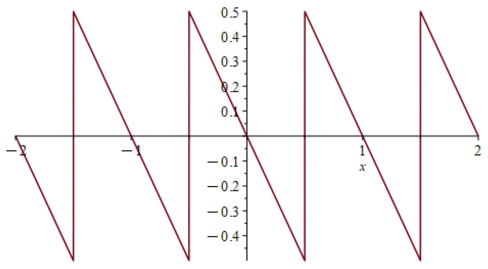
r ^ w r w is illustrated in Figure 1. Figure 1 shows that that the difference between the rounding function and the original linear function is a sawtooth wave function swt(x) with a period of 1 and an amplitude of 1.
To approximate the sawtooth wave function, we employ a novel combination of the arccos, arctan, and sine functions. Although these functions are not typically used for generating standard sawtooth or square waves, their specific combinations and transformations allow us to create a function that mimics the desired waveform. This design achieves a close approximation to the target sawtooth wave, essential for maintaining differentiability in the quantization process. The mathematical formulation of the designed sawtooth wave function s w t ( x ) * is as follows:
s w t ( x ) * = ( 1 2 arccos ( ( 1 f ) sin ( ( x 1 ) π ) ) π ) arctan ( sin ( x 1 2 ) π f ) π
The intuition behind this function’s design is to transform a standard periodic wave into the desired sawtooth shape. Specifically, the sin ( x 1 2 ) π term provides the fundamental periodic waveform. The arccos and arctan functions then act as a composite shaping operator, which stretches and sharpens the smooth sine curve to precisely mimic the linear segments and abrupt turning points of a true sawtooth wave.
This function s w t ( x ) * represents the error between the rounding operation and the identity function; by adding it back to the linear function x , we obtain the final differentiable approximation a ( x ) for the rounding function r ( x ) :
r ( x ) a ( x ) = x ( 1 2 arccos ( ( 1 f ) sin ( ( x 1 ) π ) ) π ) arctan ( sin ( x 1 2 ) π f ) π
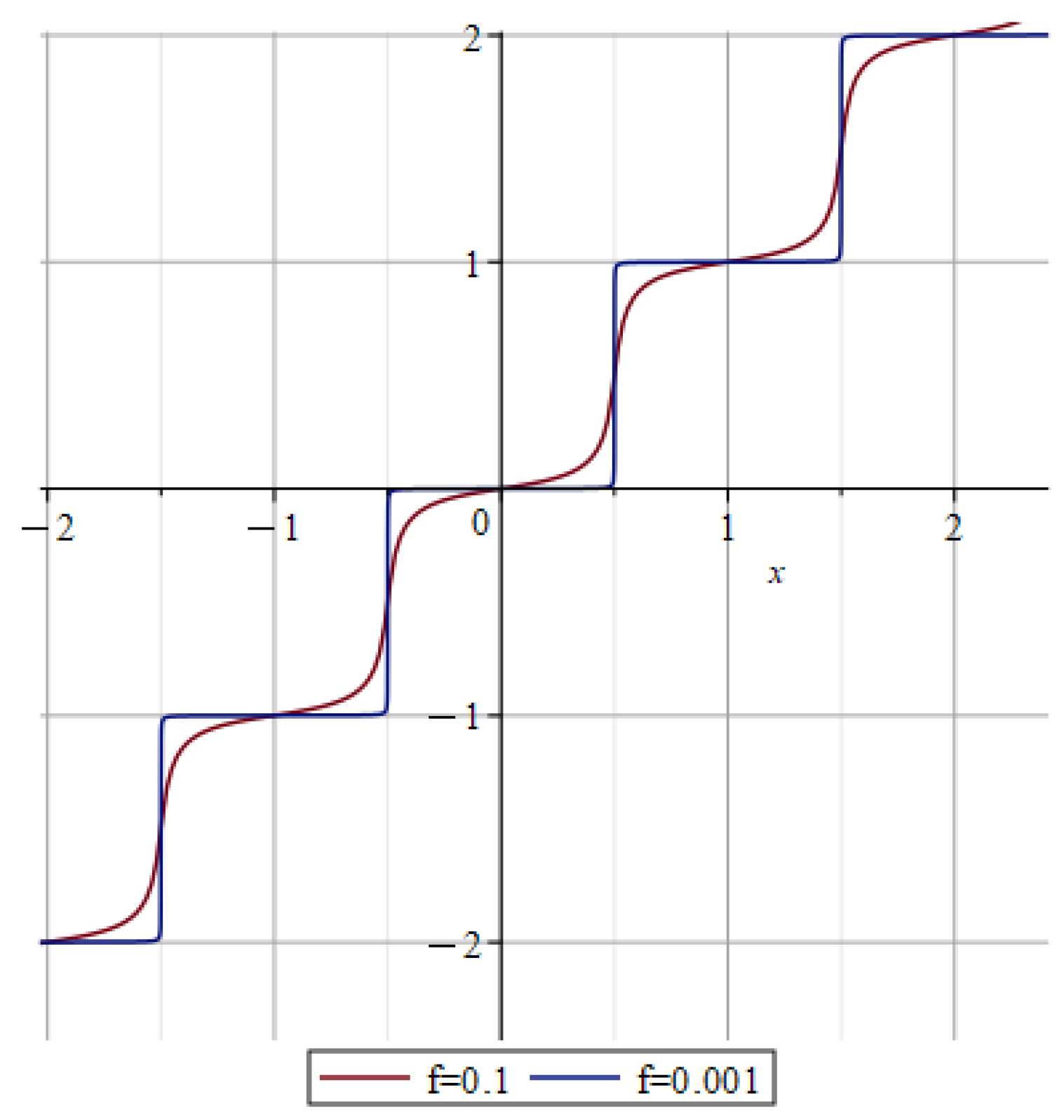
In the above equation, f is an approximate parameter that controls the smoothness of the curve. The approximate function a ( x ) is shown in the Figure 2, with red line being f = 0.1 and blue line being f = 0.001.
With respect to approximation properties and optimization stability, the proposed rounding surrogate a ( x ) uniformly approximates round ( x ) : there exists a function Φ ( f ) 0 as f 0 such that sup x | a ( x ) round ( x ) | Φ ( f ) ;
Figure 2 shows that the smaller f is, the steeper the approximate rounding operator a ( x ) and the closer it is to the original rounding operator r ( x ) . When f is sufficiently small (e.g., f = 10 3 ), a ( x ) becomes visually indistinguishable from round ( x ) at plot scale; formally, the uniform gap is bounded by Φ ( f ) . Here Φ ( f ) 0 denotes a uniform error bound that depends only on the smoothness f and satisfies Φ ( f ) 0 as f 0 . By controlling the parameter f, the differentiability of the backpropagation calculation process can be placed in a suitable numerical range. While making the model easy to converge, it effectively improves the calculation accuracy of the model and reduces the accuracy loss caused by quantization. These properties explain why decreasing f tightens the approximation while preserving well-behaved gradients, enabling stable end-to-end training.
Given the bounded-derivative property above, we adopt a ( x ) / x as a stable surrogate of round ( x ) / x during backpropagation. Then, the gradient of a ( x ) is used to approximate the gradient of the rounding operator r ( x ) = r o u n d ( x ) , as follows:
r ( x ) x a ( x ) x = 1 2 ( 1 f ) cos ( ( x 1 ) π ) arctan ( sin ( ( x 1 2 ) π ) f ) ( 1 f ) 2 sin ( ( x 1 ) π ) 2 + π ( 1 2 arccos ( ( 1 f ) sin ( ( x 1 ) π ) ) π ) cos ( ( x 1 2 ) π ) f · ( sin ( ( x 1 2 ) π ) 2 f 2 + 1 )
To further clarify the role of the smoothness parameter f, we analyze its effect from two perspectives: approximation accuracy and gradient magnitude. Since the true rounding function is discontinuous at half-integer points, the maximum pointwise error is dominated by the discontinuity region. Therefore, we use the mean approximation error to characterize the overall approximation fidelity. For a given normalized input range Ω , the empirical mean approximation error is defined as:
Φ - ( f ) = 1 N i = 1 N a f ( x i ) round ( x i )
where a f ( x ) denotes the proposed surrogate under a specific value of f, and x i Ω denotes the sampled normalized input values. Φ - ( f ) measures the average deviation between the proposed surrogate and the true rounding function within the considered normalized input range.
To characterize the gradient behavior, we further define the maximum surrogate gradient magnitude as:
G ( f ) = max x Ω a f ( x ) x
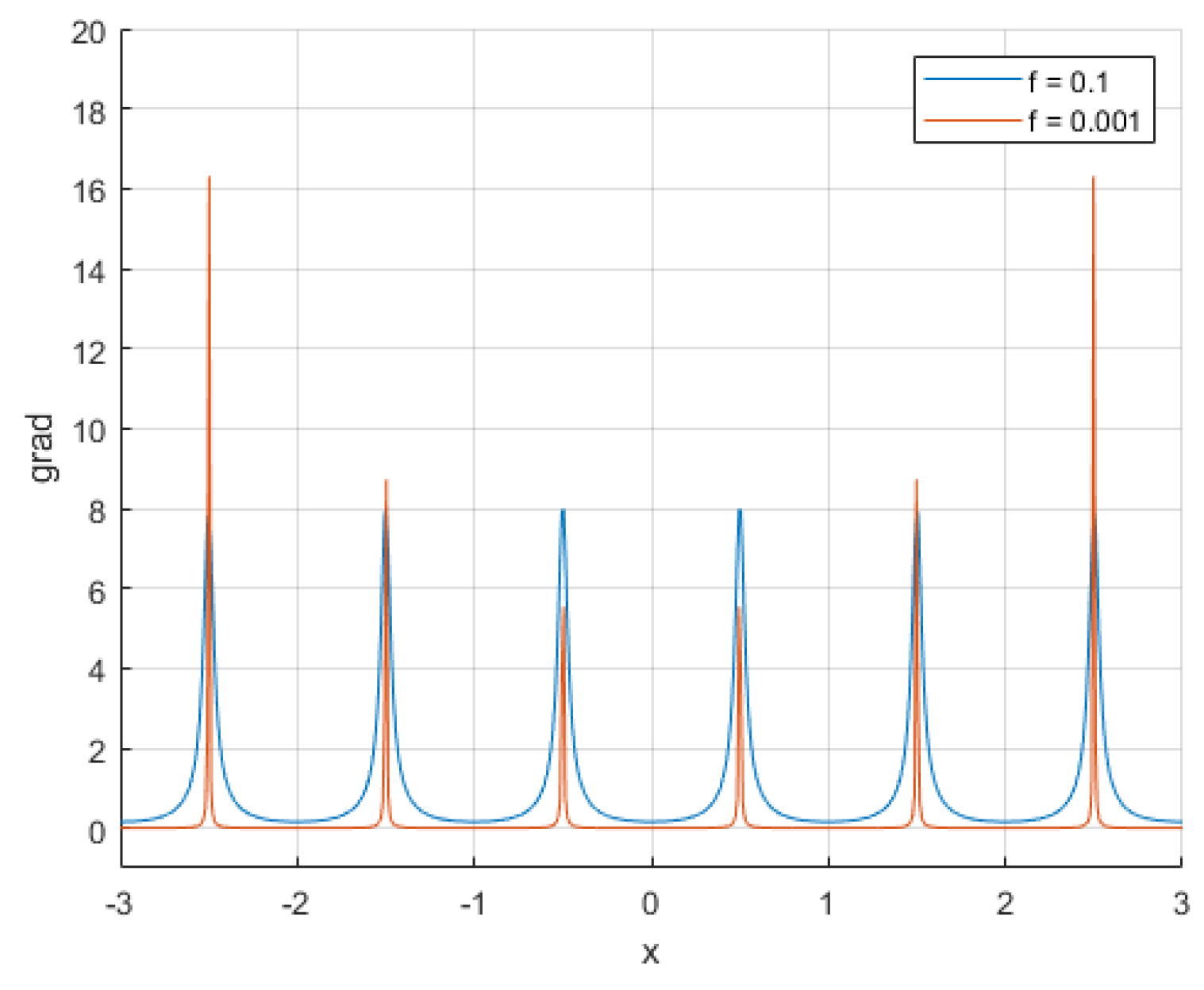
According to Equation (7), decreasing f makes the transition regions sharper and increases the peak gradient magnitude near half-integer points. Therefore, f controls a trade-off between approximation fidelity and gradient magnitude.
Table 2 reports Φ - ( f ) and G ( f ) under different values of f. As shown in Table 2, smaller f values lead to lower mean approximation error Φ - ( f ) , and they also produce larger maximum gradient magnitudes G ( f ) . This result indicates that f should not be selected solely to minimize the approximation error. Instead, it should be chosen to balance the closeness to the rounding function and the smoothness of the surrogate gradients during optimization.
Therefore, the gradient of the pseudo-quantization operator with the proposed approximate rounding operator a ( x ) with respect to the input can be expressed as Equation (10).
r w ^ r w = r w ( q w · s + D ) = r w [ r o u n d ( c l a m p ( r w , β , α ) D s ) · s + D ] = s · r w [ r o u n d ( c l a m p ( r w , β , α ) D s ) ] = s · a [ c l a m p ( r w , β , α ) D s ] [ c l a m p ( r w , β , α ) D s ] · r w [ c l a m p ( r w , β , α ) D s ] = s · a [ r w D s ] [ r w D s ] · r w [ r w D s ] , β r w α 0 , o t h e r w i s e = a [ r w D s ] [ r w D s ] , β r w α 0 , o t h e r w i s e
In which, the formula for a [ r w D s ] [ r w D s ] is as follows:
a [ r w D s ] [ r w D s ] = 1 2 ( 1 f ) cos ( ( r w D s 1 ) π ) arctan ( sin ( ( r w D s 1 2 ) π ) f ) ( 1 f ) 2 sin ( ( r w D s 1 ) π ) 2 + π ( 1 2 arccos ( ( 1 f ) sin ( ( r w D s 1 ) π ) ) π ) cos ( ( r w D s 1 2 ) π ) f · ( sin ( ( r w D s 1 2 ) π ) 2 f 2 + 1 )
In order to solve the problem that the rounding function is nondifferentiable, this paper creatively proposes a gradient approximation method to approximate the rounding function. It captures the sawtooth’s period, amplitude, and crucial sharp transitions, more effectively than generic smoothers. It enables the proposed approximate rounding operator to automatically compute gradients in the backpropagation process of quantization-aware training. In this way, the weight, quantization bit-width, and quantization parameters can be optimized independently or cooperatively, and the accuracy loss caused by quantization can be further reduced.

3.2. Quantization Parameter Optimization

Traditional quantization-aware training updates only weights and quantization parameters, calculating the quantization parameters post-weight iteration based on layer activations and weights. This decoupled update mechanism between quantization parameters and weights may lead to suboptimal results. In contrast, our proposed method enables both separate and joint optimization of weights, bitwidths, and quantization parameters, allowing more direct learning of optimal quantization configurations. This paper focuses specifically on the co-optimization mechanism between neural network model weights and quantization parameters. Other optimization methods follow fundamentally similar principles and thus will not be further discussed.
During training, pseudo-quantization is applied to both inputs and weights of each convolutional and fully connected layer. These operations estimate the data distribution and compute quantization parameters during network training. They simulate the quantization procedure and its induced error, and compensate for such errors via iterative training. For quantization-parameter calibration, we use an MSE reconstruction loss between the high-precision layer outputs and the corresponding quantized outputs. For task-level QAT/fine-tuning, the original task loss is retained. In the backpropagation phase, parameter updates are computed analytically via derivatives, instead of heuristically estimating the range of activations and weights. Pseudo-quantization yields a more uniform distribution of weights and activations, resulting in smaller accuracy degradation compared with direct post-quantization. Furthermore, constraining each layer’s output within a reasonable range effectively avoids overflow issues. Integrating quantization into network training enables reasonable weight discretization, reduces rounding-induced accuracy loss, and further improves the overall performance of quantized neural networks.
In this method, the optimization model is solved based on the generated initial quantization parameters, and the differentiable quantization parameters are automatically optimized.

3.3. Bit-Width Allocation Using Inter-Layer Sensitivity Analysis

Models with mixed bit-widths often lead to a significant decrease in model accuracy while reducing model computational complexity and improving computational efficiency. How to allocate bit widths more effectively while preserving accuracy remains an important problem. Sensitive layers and non-sensitive layers are defined based on the magnitude of accuracy loss before and after quantization. Layers with a larger decrease in accuracy are considered sensitive layers. The current basic bit-width allocation strategy is to assign higher bit-widths to sensitive layers and lower bit-widths to non-sensitive layers. Based on the hyperparameter f in the approximate round function, we propose a method for inter-layer sensitivity analysis [20].
As shown in Figure 3, it can be seen that the smaller the value of f, the sharper the derivative of the approximate round function will be. In backpropagation training, the smaller the f value of the approximate round function, the larger the calculated gradient, which leads to a larger step size for parameter updates. For sensitive layers, a larger step size often results in a significant decrease in accuracy. Therefore, we optimize the f parameter individually through fine-tuning, guiding the changes in f parameters across different layers. For sensitive layers, only by increasing the f value can we ensure an improvement in training accuracy. Non-sensitive layers exhibit much smaller parameter changes compared to sensitive layers due to their insensitivity to layer alterations.
By adaptively learning a separate f for each layer during training, we obtain layer-wise f values after fine-tuning. These learned values indicate the quantization sensitivity of different layers. Based on this observation, we assign lower bit-widths to less sensitive layers, thereby reducing the BOPS [21] of the mixed-precision model relative to a standard 8-bit configuration. First, we fix the quantization parameters and network weights to optimize the layer-wise f values and obtain the quantization sensitivity of each layer. Layers with lower sensitivity are assigned lower bit-widths. Subsequently, with the bit-widths and f values fixed, we jointly optimize the weights and quantization parameters to drive the model toward optimal convergence. In this way, our framework supports both independent and joint co-optimization of weights, bit-widths, and quantization parameters.
It should be noted that the proposed f-based sensitivity indicator is not intended to replace all existing sensitivity metrics from a theoretical perspective. Instead, it provides a lightweight, gradient-aware sensitivity measure that is naturally integrated with the proposed differentiable rounding surrogate. Compared with Hessian-based sensitivity metrics, which usually require second-order information or additional approximation, the proposed indicator can be obtained during the optimization of the surrogate parameter f. Therefore, it offers a practical alternative for guiding mixed-precision allocation within the proposed differentiable quantization framework.
Extremely low-bit settings such as W1A1 suffer from unavoidable severe accuracy loss, making them difficult for practical deployment and large-scale application. Therefore, this work mainly focuses on practical 4-bit quantization configurations, which can achieve a good balance between inference performance and compression efficiency. We leave the adaptive automatic scheduling of layer-wise f under various ultra-low-bit scenarios as a valuable direction for future research.


4. Results

We propose a continuously differentiable and automatically optimized neural network quantization method. To demonstrate the effectiveness and practicality of our approach, we conduct comparative experiments across four key dimensions. Firstly, to verify the superiority of our method, we compare our approach with the approximation functions of current state-of-the-art quantization operators, including STE, DSQ, EWGS, ReSTE, RoSTE [22], and others. Second, we validate the practical applicability of our method on embedded platforms by comparing it with the industry’s most widely used quantization frameworks [23], NVIDIA TensorRT [24] and Huawei AMCT. This comparison illustrates that our method is compatible with mainstream deep learning frameworks and hardware. Third, we compare our quantization method with leading academic approaches, such as HAWQ-v3 [25] and PyTorch 1.13.1 quantization, to showcase its superior accuracy, achieving higher performance compared to existing methods. Lastly, we evaluate our proposed bit-width allocation method against current bit-width allocation strategies, including HAWQ-v3 and BSQ [26], to demonstrate its capability not only in quantization but also in bit-width allocation. Our method supports joint optimization of bit-width allocation and quantization parameters, further enhancing model performance.

4.1. Datasets and Evaluation Metrics

For classification, we use the ImageNet dataset [27] and report top-1 accuracy. We use the top-1 accuracy to quantify the performance. That is, the prediction label takes the largest one in the last probability vector as the prediction result, if the classiffcation of the one with the highest probability in the prediction result is correct, the prediction is correct, otherwise the prediction is wrong. This dataset and evaluation metrics were also used for comparison with the state of atrs. The formula of Top-1 accuracy is given below:
Top - 1 Accuracy = Number of correct top - 1 predictions Total number of test samples
For object detection, we evaluate our method on the COCO 2017 dataset [28] using the standard MAP50 metric. We adopt MAP50 (Mean Average Precision) for performance evaluation. It considers both predicted categories and bounding box locations, where a higher value indicates better detection accuracy. The formula of AP50 is defined as:
AP 50 = k = 1 M P k × Δ R k
where AP 50 denotes the average precision calculated at an IoU threshold of 0.5, P k represents the precision corresponding to the k-th sampling point on the precision-recall curve, Δ R k indicates the recall variation between neighboring sampling points, and M is the total number of sampling points. The formula of MAP50 is defined as:
mAP 50 = 1 C i = 1 C AP 50 i
where mAP 50 is the mean average precision under the IoU threshold of 0.5, AP 50 i refers to the AP 50 value of the i-th category, and C stands for the total number of categories in the dataset.
For segmentation, we use the ISAID dataset and report Mean Intersection over Union (MIoU). The formula of MIoU is defined as:
MIoU = 1 C i = 1 C T P i T P i + F P i + F N i
where MIoU denotes the mean intersection over union across all categories, T P i , F P i and F N i represent the true positive, false positive and false negative pixels of the i-th category, respectively, and C is the total number of semantic categories. In experiments related to LLMs, the publicly available Reddit TL;DR dataset was used. The evaluation metric Rouge-N works by comparing machine-generated summaries (candidate summaries) with one or more human-generated, ideal summaries (reference summaries), and scores their similarity based on the overlapping units.
The formula of ROUGE-1 is defined as:
ROUGE - 1 = Match 1 - gram Total 1 - gram
where Match 1 - gram represents the number of matched unigrams between candidate and reference summaries, and Total 1 - gram denotes the total number of unigrams in reference summaries.
The formula of ROUGE-2 is defined as:
ROUGE - 2 = Match 2 - gram Total 2 - gram
where Match 2 - gram refers to the number of matched bigram phrases, and Total 2 - gram is the total number of bigram phrases in reference summaries.
The formula of Rouge-L is defined as:
Rouge - L = ( 1 + β 2 ) · P · R β 2 · P + R
where P and R denote the precision and recall calculated based on the longest common subsequence, and β is a balance coefficient between precision and recall.
The formula of ROUGE-Lsum is defined as:
ROUGE - Lsum = 1 S s = 1 S ROUGE - L s
where ROUGE - L s is the sentence-level ROUGE-L score of the s-th sentence, and S is the total number of sentences in the evaluated document.

4.2. Implementation Details

In the comparative experiments with other industry-standard quantization operators’ approximation functions, we compared our approach with several existing approximation functions, such as STE, DSQ, EWGS, ReSTE, DoReFa, LQ-Net, IRNet, and others. To ensure the fairness of the experiments, we only replaced the implementation modules of different quantization approximation functions, while keeping other model training settings unchanged. We conducted model accuracy comparisons with multiple bit-widths on the CIFAR-10 [29] dataset to demonstrate the superiority of our method. The proposed testing method is also extended to the quantization of large language models. Similarly, we only replace the implementation module of the approximation function while keeping all other training settings unchanged. On the Qwen2.5-0.5B [30] and Pythia-1B [31] models, the approximation function proposed in this work outperforms other approximation functions in terms of accuracy.
In our experimental comparison with mainstream industrial quantization frameworks including NVIDIA TensorRT and Huawei AMCT, we standardize the quantization workflow for fair comparison. The entire quantization process is unified into two stages: model calibration on the host platform using a validation dataset to determine proper quantization parameters, and model conversion and deployment onto embedded platforms for accuracy evaluation. For TensorRT, we first follow the standard PyTorch-based TensorRT quantization pipeline to conduct calibration and generate a native INT8 quantized ONNX model with default quantization parameters. Based on this baseline model, we apply our proposed quantization parameter optimization scheme for fine-tuning to obtain optimized quantization parameters. Following the scaling format of native TensorRT quantization, we replace the original scaling factors in the ONNX model with our optimized parameters before deployment. During inference, TensorRT INT8 kernels load the updated scaling factors to execute integer computation. For Huawei AMCT, we adopt the official amct-pytorch toolkit for model quantization. After obtaining the baseline quantized model via AMCT default calibration, we replace both the scaling factors and zero-point values in the model with our optimized parameters. The Ascend NPU INT8 kernels then load these parameters to perform asymmetric quantization. Most mainstream embedded platforms primarily support only INT8 computation and generally adopt post-training quantization (PTQ). TensorRT employs symmetric quantization, whereas AMCT uses asymmetric quantization, with the core difference lying in whether the zero-point is fixed at zero. To fairly compare the native quantization schemes across platforms, we adopt different initialization strategies for quantization parameters. Specifically, we initialize TensorRT with symmetric quantization and fix the zero-point of each layer during parameter optimization. For AMCT, we initialize parameters under asymmetric quantization and allow all quantization parameters to be fully optimized in the optimization stage.
Our proprietary quantization method differs from quantization-aware training (QAT) [32] as it does not require a large dataset or multiple training epochs. We choose the Nvidia Titan GPU for host-platform training. For classification models, the batch size for fine-tuning quantization parameters is 16; for detection model yolov5s and segmentation model unet, the batch size for fine-tuning is 4, and only the first 100 batches of images per epoch are used to optimize the model’s quantization parameters. For different models, the learning rate is set to 10 4 , and the model training is set for 10 epochs, with the hyperparameter f for our proposed approximate round function set to 0.9.
When comparing with state-of-the-art model quantization algorithms HAWQ-v3 and PyTorch, HAWQ-v3 is a quantization-aware training (QAT), and PyTorch uses post-training quantization algorithm (PTQ). In the comparison experiment with HAWQ-v3, unlike the experimental models based on embedded platforms, HAWQ-v3 uses pre-trained models from pytorchcv for classification, we use the default hyperparameter settings of HAWQ-v3: the learning rate is set to 10 4 , the training batch size is set to 128, and the learning rate decay is set to 0.1, decaying every 30 epochs. In the comparison experiment with PyTorch, the quantization configuration chosen is “fbgemm”, which mainly targets INT8 quantization for X86 platforms. The calibration code is implemented through torch.fx, and our method’s parameter settings are consistent with those in the aforementioned embedded platform experiments.
In the bit-width allocation comparison experiments, we compare our method with industry bit-width allocation methods HAWQ-v3 and BSQ on different datasets. HAWQ provides multiple mixed bit-width allocation results for multiple models with different bit operations. To highlight the superiority of our bit-width allocation method, we select the bit-width allocation result with the smallest bit operations for accuracy comparison, and we still choose the default hyperparameter settings of HAWQ-v3. In the comparison experiment with BSQ, based on the ResNet20 [33] model, we conduct comparisons with different weight bit-widths under input bit-widths of 4 bit and 8 bit. The BSQ quantization method is divided into two steps: training to search for bit-width and fine-tuning quantization parameters. The training to search for bit-width sets the training epochs to 350, the learning rate to 0.1, the training batch size to 128, and the learning rate decay to 0.1, decaying every 250 epochs. The fine-tuning quantization parameters set the training epochs to 300 and the learning rate to 0.01. Unlike our experiments optimizing quantization parameters, where we fixed the f parameter and the model’s original weights, optimizing only the model’s quantization parameters, in our bit-width allocation experiments, we fixed the quantization parameters and original weights, optimizing only the f parameter.

4.3. Validation of Quantization Approximation Functions

We have conducted a comprehensive comparison with other quantization approximation functions. To ensure the fairness of the experiments, we directly replaced the implementation modules of other quantization approximation functions. We trained the parameters on the CIFAR-10 dataset using ResNet-20,Since the comparative bit-widths of current mainstream methods are W1A32 and W1A1 (where WxAy specifically denotes a weight bit-width of x bits and an activation bit-width of y bits), this experiment compares the accuracy with current industry-standard quantization approximation functions under these two bit-width settings. These functions include STE, DSQ, EWGS, ReSTE, DoReFa, and others. Our method achieved the lowest quantization loss in all comparisons. The specific experimental results are shown in Table 3. As can be seen from the table, our method based on ResNet-20 achieves the best accuracy compared with other state-of-the-art methods under different bit-width conditions. Under the W1A1 bit-width setting, our quantization accuracy drops by only 5.0% compared to the baseline accuracy, which is significantly lower than the quantization loss of other methods. Under the W1A32 bit-width setting, our quantization accuracy drops by just 0.37% compared to the baseline accuracy.
By modifying the backpropagation function of the STE method, we also applied our proposed approximation function to the quantization accuracy comparison of LLMs. As shown in Table 4, we conducted 4-bit quantization-aware supervised fine-tuning (QA-SFT) on the Reddit TL;DR dataset using the Qwen-0.5b and Pythia-1b models. Our method achieved the optimal accuracy in terms of Rouge-N evaluation metrics.
We conduct zero-shot evaluations on Qwen-0.5B and Pythia-1B using three mainstream commonsense reasoning benchmarks, including HellaSwag, PIQA, and WinoGrande. In existing research on LLM quantization and quantization-aware training, zero-shot evaluation on these benchmarks has become a standard mainstream paradigm, which can fully verify the generalization ability of the proposed method across various downstream tasks. Both the original full-precision model and the quantized model are fine-tuned on the Reddit TL; DR dataset, and their accuracy is evaluated on the three mainstream knowledge reasoning benchmarks. Comprehensive evaluations on typical small-scale LLMs with multiple standard zero-shot benchmarks are sufficient to validate the effectiveness and applicability of our quantization framework. Specifically, normalized accuracy (acc_norm) is adopted as the evaluation metric for all tasks. As shown in Table 5, our method achieves superior performance on all zero-shot benchmark tasks compared with the STE and RoSTE baselines.
To demonstrate the effectiveness of our method, we conducted a comparative study within a baseline project based on ResNet20, evaluating four different approximation methods. We performed quantization-aware training for each method and measured the time required per iteration. As shown in Table 6, although our approach may slightly reduce training speed, it delivers a significant improvement in quantization accuracy.
Based on the above large-scale LLM experimental settings, we further quantitatively analyze the per-iteration training computational overhead of different quantization approximation methods. Table 7 reports the average per-iteration training latency of STE, RoSTE, and our method on Qwen-0.5B and Pythia-1B with a fixed batch size of 8. Compared with the standard STE baseline, our method introduces extra computational cost from trigonometric functions and their derivative calculations in both forward and backward passes. Specifically, on Qwen-0.5B, the per-iteration latency increases from 507.0 ms (STE) to 871.0 ms; on Pythia-1B, the latency rises from 619.8 ms (STE) to 1555.0 ms. Moreover, the computational overhead exhibits an obvious scaling trend with model size. As the model scale grows from 0.5B to 1B parameters, the relative latency increment of our method becomes larger, because more transformer layers and quantization modules bring more trigonometric operation calculations during QAT. Nevertheless, the higher training cost is a reasonable tradeoff for substantial quantization accuracy gains.
Please note that, all trigonometric operations ( sin , arccos , arctan ) appear only during training to enable gradient flow. At inference, we discard a ( · ) and use standard integer arithmetic with fixed ( s , D ) and round ( · ) ; therefore no extra runtime latency.

4.4. Practical Validation on Embedded Platforms

In this experiment, we compared the accuracy of our method with NVIDIA’s and Huawei’s native quantization APIs on the Jetson Xavier NX (NVIDIA, Santa Clara, CA, USA) platform and the Atlas200 DK (Huawei, Shenzhen, China) platform, respectively. All models in this experiment adopted the W8A8 bit-width configuration.
As shown in Table 8, on the Jetson Xavier NX platform, we conducted accuracy comparison experiments for classification models based on ResNet50, MobileNetV2 [34], and MobileNetV1 [35]. Among them, our method outperformed TensorRT by 0.02 points on the ResNet50 classification model, by 0.35 points on the MobileNetV2 classification model, and by 0.38 points on the MobileNetV1 classification model. In the object detection experiment, based on the classic detection network YOLOV5s [36], our method outperformed TensorRT’s quantization method by 3.66 points. In the object segmentation experiment, based on the UNet [37] segmentation network, our method outperformed TensorRT’s quantization method by 2.71 points. Note that our training graph contains trigonometric functions only to enable gradient flow; at inference we discard the surrogate a ( · ) and execute standard INT arithmetic with the exported scales/zero-points. Consequently, the deployment procedure (calibration → conversion) and the runtime kernels are identical in nature to those of TensorRT/AMCT, and our approach incurs no extra latency/memory/energy overhead. The only difference is that we export the calibrated parameters in multiple backend-compatible formats, improving cross-platform portability.
On the Atlas200 DK embedded inference platform, as shown in Table 9, on the Atlas200 DK embedded inference platform, our method achieved higher accuracy than AMCT. On the ResNet50 classification model, our method’s accuracy was 0.33 points higher than AMCT quantization method. On the MobileNetV1 and MobileNetV2 models, our method was 0.17 and 0.22 points higher, respectively. On the YOLOV5s model, our method was 0.03 points higher than AMCT quantization method, and on the UNet model, it was 0.38 points higher than AMCT quantization method.

4.5. High-Accuracy Validation Against State-of-the-Art Methods

This experiment primarily compares the accuracy of the classic academic quantization method HAWQ-v3 and PyTorch’s native quantization method torch.quantize across three different visual tasks: classification, detection, and segmentation, with HAWQ focusing only on mainstream classification models for quantization comparison.
As shown in Table 10, our quantization method achieved higher accuracy on the ResNet series of models compared to both HAWQ-v3 and torch.quantize, with an average quantization accuracy that is 0.26 higher than the second place. In the MobileNet series, our method’s quantization accuracy is significantly better than that of torch.quantize, with a 1.03 higher accuracy on the MobileNetV2. On the YOLOV5s detection model and UNet segmentation model, our method’s accuracy is also superior to that of torch.quantize’s quantization method.

4.6. Validation of Bit-Width Allocation Capabilities

In the bit-width allocation experiment, the HAWQ-v3 method is primarily based on classification models, and conducts comparison tests on the ImageNet dataset, while the BSQ method only provides comparisons based on ResNet20 on the CIFAR-10 dataset. Therefore, to ensure the fairness of the experiment, we choose different benchmarks to compare these two methods.
To validate the proposed f-based sensitivity indicator against standard sensitivity metrics, we compare it with HAWQ-v3, a representative Hessian-based mixed-precision quantization method.
As shown in Table 11, the second column represents the precision of the bit-width allocated to the model. bit operations can assess the total number of bit operations required by a model or algorithm when processing data. Our method achieved the best accuracy on three classification models, and under the condition of similar bit operations, our method outperformed the HAWQ-v3 method by 7.49 points on MobileNetV2.
As shown in Table 12, BSQ only searches for weight bit-width with activation bit-width fixed at 4/8-bit. Under the condition of similar bit operations, our accuracy is 0.71 points higher than the BSQ method in the comparison with an activation bit-width of 4-bit.
To further verify the effectiveness of the proposed inter-layer sensitivity analysis and mixed bit-width allocation strategy, we supplement additional ablation experiments in this section. A baseline setting without layer-wise sensitivity optimization is introduced, where all network layers adopt a unified fixed hyperparameter f and a consistent 8-bit quantization configuration is adopted for the entire network.In this case, the layer differentiation characteristic derived from diverse f optimization is eliminated, and the adaptive mixed bit-width allocation is no longer performed.
Table 13 shows that the unified 8-bit scheme achieves higher accuracy but requires substantially higher BOPS. In contrast, the proposed sensitivity-guided mixed-precision scheme significantly reduces BOPS while retaining acceptable accuracy. This indicates that the proposed inter-layer sensitivity analysis helps improve the accuracy–BOPS trade-off, rather than simply maximizing accuracy under a fixed 8-bit setting. Therefore, the optimized f-based layer sensitivity provides practical guidance for assigning lower bit-widths to less sensitive layers and preserving higher bit-widths for more sensitive layers.

4.7. Sensitivity Analysis of Hyperparameter f

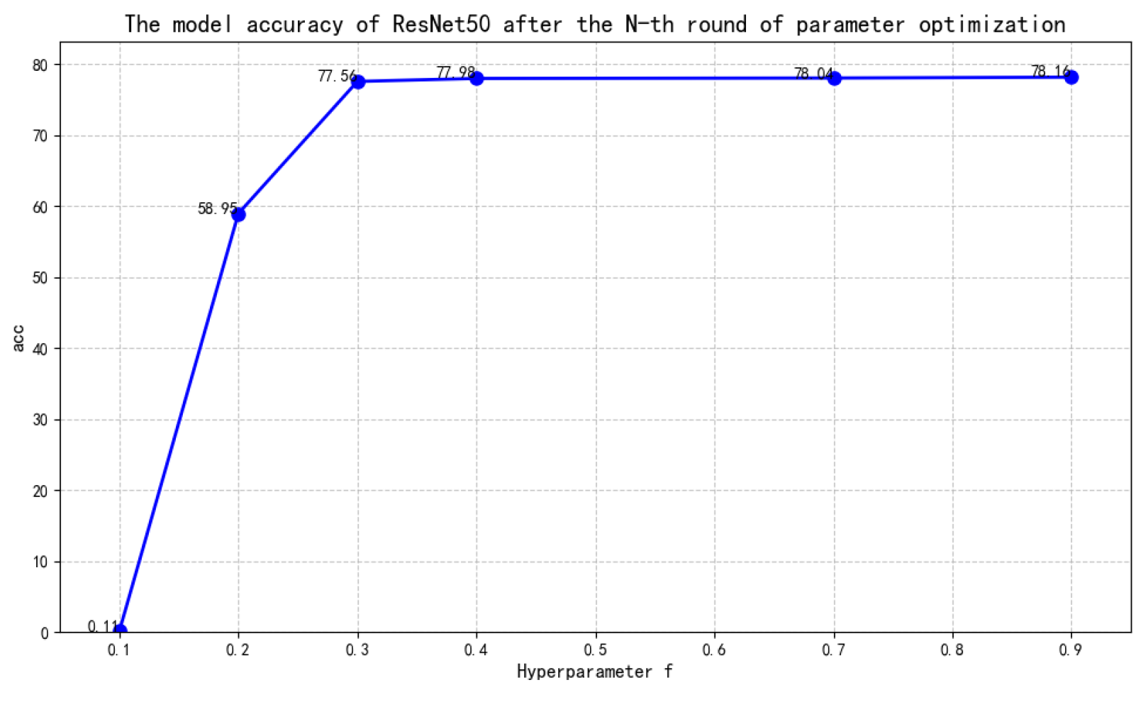
In our proposed method, the hyperparameter f can adjust the degree to which the approximate function approaches the real round function. The smaller the f value, the smaller the error between the approximate function and the round function. When f = 1, the approximate function is equivalent to STE. Although a smaller f reduces the approximation error, it may also lead to unstable optimization because the surrogate gradients become excessively sharp during backpropagation. Therefore, an appropriate f is crucial for the stable convergence of our method.
As shown in Figure 4, we trained ResNet50 on the ImageNet dataset for 10 epochs. When f = 0.1, the quantized top-1 accuracy of the model is 0.11. As the f value increases, the quantization accuracy gradually improves. When f = 0.3, the quantization accuracy has approached the accuracy of the unquantized model. Meanwhile, it can be seen from the figure that when f ranges from 0.3 to 0.9, the final quantization accuracy of the model is close to that of the unquantized model, suggesting that the model is less sensitive to parameter f within a broad range; only when f takes extreme values does the model performance degrade.
To further clarify which components contribute to the overall improvement, we summarize the ablation evidence from four aspects: First, the contribution of the proposed approximation function is evaluated in Table 3, where only the gradient approximation function is replaced while the other training settings are kept unchanged. The comparison with STE, DSQ, EWGS, and ReSTE shows that the proposed differentiable surrogate reduces quantization loss under both W1A1 and W1A32 settings. Second, the effect of the smoothness parameter f is analyzed in Section 4.7 and in the additional analysis after Equation (7). The results show that f controls the trade-off between approximation accuracy and gradient magnitude. Extremely small f values lead to sharp gradients, whereas moderate values provide a more stable balance between approximation fidelity and optimization behavior. Third, the contribution of the inter-layer sensitivity-guided bit-width allocation is evaluated in Table 12. Compared with the unified 8-bit setting, the proposed mixed-precision strategy significantly reduces BOPS while retaining acceptable accuracy, indicating that the learned f-based sensitivity provides practical guidance for bit-width allocation. Finally, the effect of quantization-parameter optimization is evaluated in the embedded-platform experiments. Under the same TensorRT/AMCT INT8 backend execution environment, the baseline uses calibration-derived quantization parameters, whereas our method uses optimized parameters exported into backend-compatible formats. This comparison evaluates whether the proposed optimization strategy can provide better quantization parameters without modifying the backend inference kernels. Overall, these experiments isolate the effects of the approximation function, the smoothness parameter f, the sensitivity-guided bit-width allocation, and the quantization-parameter optimization strategy, showing that the final performance gain is contributed by these components from different perspectives.

5. Conclusions

We introduced a novel differentiable quantization method that approximates the non-differentiable rounding operation with a continuous function. This allows end-to-end gradient-based optimization of both weights and quantization parameters, including bit-width allocation. Experiments showed that our approach surpasses existing industrial approximations and improves post-quantization accuracy on embedded platforms by up to 3.66%. Compared to other state-of-the-art algorithms such as HAWQ-v3 and torch.quantize, our method achieves higher accuracy while retaining fewer bit operations than competing bit-width allocation strategies. These results highlight its potential for efficient, accurate neural network deployment in resource-constrained environments.

Author Contributions

Conceptualization, Z.M. and Y.Y.; methodology, Y.Y., Z.M., L.W., Y.W. and C.Y.; software, Y.Y.; validation, Y.Y.; formal analysis, Y.Y. and Z.M.; investigation, Y.Y., Z.M., L.W., Y.W. and C.Y.; data curation, Y.Y., L.W. and Y.W.; writing—original draft preparation, Y.Y. and Y.W.; writing—review and editing, Z.M.; visualization, Y.Y. and Y.W.; supervision, Z.M. and Y.Y.; project administration, Z.M.; All authors have read and agreed to the published version of the manuscript.

Funding

This research received no external funding.

Institutional Review Board Statement

Not applicable.

Informed Consent Statement

Not applicable.

Data Availability Statement

The raw data supporting the conclusions of this article will be made available by the authors on request.

Acknowledgments

The authors wish to thank all those who provided assistance during this research.

Conflicts of Interest

The authors declare no conflicts of interest. The funders had no role in the design of the study; in the collection, analyses, or interpretation of data; in the writing of the manuscript, or in the decision to publish the results.

Abbreviations

The following abbreviations are used in this manuscript:
STEStraight-Through Estimator
EWGSElement-wise Gradient Scaling
DSQDifferentiable Soft Quantization
ReSTERectified Straight-Through Estimator
BOPSBit Operations
MAPMean Average Precision
MIOUMean Intersection Over Union
PTQPost-training Quantization
QATQuantization-aware Training
AMCTAscend Model Compression Toolkit
QA-SFTQuantization-aware Supervised Fine-tuning

References

  1. Gholami, A.; Kim, S.; Dong, Z.; Yao, Z.; Mahoney, M.W.; Keutzer, K. A survey of quantization methods for efficient neural network inference. In Low-Power Computer Vision; Chapman and Hall/CRC: Boca Raton, FL, USA, 2022; pp. 291–326. [Google Scholar]
  2. Tampuu, A.; Matiisen, T.; Semikin, M.; Fishman, D.; Muhammad, N. A survey of end-to-end driving: Architectures and training methods. IEEE Trans. Neural Netw. Learn. Syst. 2020, 33, 1364–1384. [Google Scholar] [CrossRef] [PubMed]
  3. Adrian, A.I.; Ismet, P.; Petru, P. An overview of intelligent surveillance systems development. In Proceedings of the 2018 International Symposium on Electronics and Telecommunications (ISETC); IEEE: Piscataway, NJ, USA, 2018; pp. 1–6. [Google Scholar]
  4. Tang, L.; Ma, Z.; Li, S.; Wang, Z. The present situation and developing trends of space-based intelligent computing technology. Microelectron. Comput. 2022, 39, 1–8. [Google Scholar]
  5. Majumder, S.; Mondal, T.; Deen, M.J. Wearable sensors for remote health monitoring. Sensors 2017, 17, 130. [Google Scholar] [CrossRef] [PubMed]
  6. Bengio, Y.; Léonard, N.; Courville, A. Estimating or propagating gradients through stochastic neurons for conditional computation. arXiv 2013, arXiv:1308.3432. [Google Scholar] [CrossRef]
  7. Hao, R.; Yang, X. Multiple-output quantile regression neural network. Stat. Comput. 2024, 34, 89. [Google Scholar] [CrossRef]
  8. Yang, J.; Liu, Y.; Wang, W.; Wu, H.; Chen, Z.; Ma, X. PATNAS: A path-based training-free neural architecture search. IEEE Trans. Pattern Anal. Mach. Intell. 2024, 47, 1484–1500. [Google Scholar] [CrossRef] [PubMed]
  9. Lee, J.; Kim, D.; Ham, B. Network quantization with element-wise gradient scaling. In Proceedings of the IEEE/CVF Conference on Computer Vision and Pattern Recognition, Virtual, 19–25 June 2021; pp. 6448–6457. [Google Scholar]
  10. Zhou, S.; Wu, Y.; Ni, Z.; Zhou, X.; Wen, H.; Zou, Y. Dorefa-net: Training low bitwidth convolutional neural networks with low bitwidth gradients. arXiv 2016, arXiv:1606.06160. [Google Scholar]
  11. Zhang, D.; Yang, J.; Ye, J.; Hua, G. Learned quantization for highly accurate and compact deep neural networks. arXiv 2018, arXiv:1807.10029. [Google Scholar] [CrossRef]
  12. Qin, H.; Gong, R.; Liu, X.; Shen, M.; Wei, Z.; Yu, F.; Song, J. Forward and backward information retention for accurate binary neural networks. In Proceedings of the IEEE/CVF Conference on Computer Vision and Pattern Recognition, Virtual, 14–19 June 2020; pp. 2250–2259. [Google Scholar]
  13. Yang, J.; Shen, X.; Xing, J.; Tian, X.; Li, H.; Deng, B.; Huang, J.; Hua, X.S. Quantization networks. In Proceedings of the IEEE/CVF Conference on Computer Vision and Pattern Recognition, Long Beach, CA, USA, 16–20 June 2019; pp. 7308–7316. [Google Scholar]
  14. Gong, R.; Liu, X.; Jiang, S.; Li, T.; Hu, P.; Lin, J.; Yu, F.; Yan, J. Differentiable soft quantization: Bridging full-precision and low-bit neural networks. In Proceedings of the IEEE/CVF International Conference on Computer Vision, Seoul, Republic of Korea, 27 October–2 November 2019; pp. 4852–4861. [Google Scholar]
  15. Wu, X.M.; Zheng, D.; Liu, Z.; Zheng, W.S. Estimator meets equilibrium perspective: A rectified straight through estimator for binary neural networks training. In Proceedings of the IEEE/CVF International Conference on Computer Vision, Paris, France, 2–6 October 2023; pp. 17055–17064. [Google Scholar]
  16. Moon, J.; Kim, D.; Cheon, J.; Ham, B. Instance-aware group quantization for vision transformers. In Proceedings of the IEEE/CVF Conference on Computer Vision and Pattern Recognition, Seattle, WA, USA, 17–21 June 2024; pp. 16132–16141. [Google Scholar]
  17. Guan, Z.; Huang, H.; Su, Y.; Huang, H.; Wong, N.; Yu, H. Aptq: Attention-aware post-training mixed-precision quantization for large language models. In Proceedings of the 61st ACM/IEEE Design Automation Conference, San Francisco, CA, USA, 23–27 June 2024; pp. 1–6. [Google Scholar]
  18. Fu, M.; Yu, H.; Shao, J.; Zhou, J.; Zhu, K.; Wu, J. Quantization without tears. In Proceedings of the Computer Vision and Pattern Recognition Conference, Nashville, TN, USA, 11–15 June 2025; pp. 4462–4472. [Google Scholar]
  19. LeCun, Y.; Bottou, L.; Bengio, Y.; Haffner, P. Gradient-based learning applied to document recognition. Proc. IEEE 1998, 86, 2278–2324. [Google Scholar] [CrossRef]
  20. Iooss, B.; Lemaître, P. A review on global sensitivity analysis methods. In Uncertainty Management in Simulation-Optimization of Complex Systems: Algorithms and Applications; Springer: Berlin/Heidelberg, Germany, 2015; pp. 101–122. [Google Scholar]
  21. Rokh, B.; Azarpeyvand, A.; Khanteymoori, A. A comprehensive survey on model quantization for deep neural networks in image classification. ACM Trans. Intell. Syst. Technol. 2023, 14, 1–50. [Google Scholar] [CrossRef]
  22. Wei, Q.; Yau, C.Y.; Wai, H.T.; Zhao, Y.K.; Kang, D.; Park, Y.; Hong, M. Roste: An efficient quantization-aware supervised fine-tuning approach for large language models. arXiv 2025, arXiv:2502.09003. [Google Scholar]
  23. Cheng, Y.Q.; He, Z.Z.; Ma, Z.; Bi, R.X.; Mao, Y.H. Intelligent target detection algorithm for embedded FPGA. Microelectron. Comput. 2021, 38, 87–92. [Google Scholar]
  24. Zhou, Y.; Yang, K. Exploring TensorRT to improve real-time inference for deep learning. In Proceedings of the 2022 IEEE 24th Int Conf on High Performance Computing & Communications; 8th Int Conf on Data Science & Systems; 20th Int Conf on Smart City; 8th Int Conf on Dependability in Sensor, Cloud & Big Data Systems & Application (HPCC/DSS/SmartCity/DependSys); IEEE: Piscataway, NJ, USA, 2022; pp. 2011–2018. [Google Scholar]
  25. Yao, Z.; Dong, Z.; Zheng, Z.; Gholami, A.; Yu, J.; Tan, E.; Wang, L.; Huang, Q.; Wang, Y.; Mahoney, M.; et al. Hawq-v3: Dyadic neural network quantization. In Proceedings of the International Conference on Machine Learning, Virtual, 18–24 July 2021; pp. 11875–11886. [Google Scholar]
  26. Yang, H.; Duan, L.; Chen, Y.; Li, H. BSQ: Exploring bit-level sparsity for mixed-precision neural network quantization. arXiv 2021, arXiv:2102.10462. [Google Scholar]
  27. Deng, J.; Dong, W.; Socher, R.; Li, L.J.; Li, K.; Li, F. Imagenet: A large-scale hierarchical image database. In Proceedings of the 2009 IEEE Conference on Computer Vision and Pattern Recognition; IEEE: Piscataway, NJ, USA, 2009; pp. 248–255. [Google Scholar]
  28. Lin, T.Y.; Maire, M.; Belongie, S.; Hays, J.; Perona, P.; Ramanan, D.; Dollár, P.; Zitnick, C.L. Microsoft coco: Common objects in context. In Proceedings of the Computer Vision–ECCV 2014: 13th European Conference, Zurich, Switzerland, 6–12 September 2014; Proceedings, Part V 13; Springer: Berlin/Heidelberg, Germany, 2014; pp. 740–755. [Google Scholar]
  29. Recht, B.; Roelofs, R.; Schmidt, L.; Shankar, V. Do cifar-10 classifiers generalize to cifar-10? arXiv 2018, arXiv:1806.00451. [Google Scholar] [CrossRef]
  30. Xu, J.; Guo, Z.; He, J.; Hu, H.; He, T.; Bai, S.; Chen, K.; Wang, J.; Fan, Y.; Dang, K.; et al. Qwen2. 5-omni technical report. arXiv 2025, arXiv:2503.20215. [Google Scholar]
  31. Biderman, S.; Schoelkopf, H.; Anthony, Q.G.; Bradley, H.; O’Brien, K.; Hallahan, E.; Khan, M.A.; Purohit, S.; Prashanth, U.S.; Raff, E.; et al. Pythia: A suite for analyzing large language models across training and scaling. In Proceedings of the International Conference on Machine Learning, Honolulu, HI, USA, 23–29 July 2023; pp. 2397–2430. [Google Scholar]
  32. Jacob, B.; Kligys, S.; Chen, B.; Zhu, M.; Tang, M.; Howard, A.; Adam, H.; Kalenichenko, D. Quantization and training of neural networks for efficient integer-arithmetic-only inference. In Proceedings of the IEEE Conference on Computer Vision and Pattern Recognition, Salt Lake City, UT, USA, 18–22 June 2018; pp. 2704–2713. [Google Scholar]
  33. He, K.; Zhang, X.; Ren, S.; Sun, J. Deep residual learning for image recognition. In Proceedings of the IEEE Conference on Computer Vision and Pattern Recognition, Las Vegas, NV, USA, 26 June–1 July 2016; pp. 770–778. [Google Scholar]
  34. Sandler, M.; Howard, A.; Zhu, M.; Zhmoginov, A.; Chen, L.C. Mobilenetv2: Inverted residuals and linear bottlenecks. In Proceedings of the IEEE Conference on Computer Vision and Pattern Recognition, Salt Lake City, UT, USA, 18–22 June 2018; pp. 4510–4520. [Google Scholar]
  35. Howard, A.G.; Zhu, M.; Chen, B.; Kalenichenko, D.; Wang, W.; Weyand, T.; Andreetto, M.; Adam, H. MobileNets: Efficient convolutional neural networks for mobile vision applications. arXiv 2017, arXiv:1704.04861. [Google Scholar] [CrossRef]
  36. Liu, J.; Liu, Z. YOLOv5s-BC: An improved YOLOv5s-based method for real-time apple detection. J. Real-Time Image Process. 2024, 21, 88. [Google Scholar] [CrossRef]
  37. Ronneberger, O.; Fischer, P.; Brox, T. U-net: Convolutional networks for biomedical image segmentation. In Proceedings of the Medical Image Computing and Computer-Assisted Intervention–MICCAI 2015: 18th International Conference, Munich, Germany, 5–9 October 2015; Proceedings, Part III 18; Springer: Berlin/Heidelberg, Germany, 2015; pp. 234–241. [Google Scholar]
Figure 1. Desired Sawtooth wave function s w t ( x ) .
Applsci 16 05281 g001
Figure 2. An approximation of the round function.
Applsci 16 05281 g002
Figure 3. The gradient change curve of a ( x ) . Varies with different f values.
Applsci 16 05281 g003
Figure 4. Sensitivity analysis experiment of hyperparameter f based on ResNet50.
Applsci 16 05281 g004
Table 1. A comparison of quantization approximation functions. The flexibility indicates that the approximation method should be capable of adjusting the degree of estimation error and gradient stability. Our method not only meets the requirements of flexible property but also everywhere differentiable, enabling parameters to converge more rapidly.
EstimatorsFormulaTypeFlexibleEverywhere Differentiable
STE [6] f ( x ) = x Identity functionNot flexibleDifferentiable
EWGS [9] f ( x ) = x · ( 1 + δ · s i g n ( x ) · ( x n x ) ) /Little flexibleNon-differentiable
QN [13]  f ( x ) = 1 1 + e x p ( T · x ) Sigmoid-alikeLittle flexibleNon-differentiable
DSQ [14] f ( x ) = l + Δ ( i + ( s · tanh ( k ( x m ) ) + 1 ) / 2 ) Tanh-alikeLittle flexibleNon-differentiable
ReSTE [15] f ( x ) = s i g n ( x ) | x | 1 o Power functionFlexibleNon-differentiable
Ours f ( x ) = x ( 1 2 arccos ( ( 1 f ) sin ( ( x 1 ) π ) ) π ) π · arctan ( sin ( x 1 2 ) π f ) /FlexibleDifferentiable
Table 2. Effect of f on mean approximation error and maximum gradient magnitude.
fMean Approximation Error ( Φ - (f))G(f)Observation
0.0010.00235972.52Very close to rounding almost everywhere, but with extremely sharp gradients
0.010.0162191.99Small approximation error, but with large gradient peaks
0.10.087918.13Moderate approximation error and reduced gradient peaks
0.30.163632.65Balanced approximation accuracy and gradient magnitude
0.50.203411.67Smoother gradients with increased approximation bias
0.90.243851.07Smoothest gradients but larger approximation bias
Table 3. Comparison of quantization approximation functions. Under both bit-width conditions, our method demonstrates the smallest accuracy degradation and the most stable results (lowest variance) on the CIFAR-10 dataset. Each value in the table represents the result obtained from multiple runs, and is expressed in the form of mean ± standard deviation. The values in parentheses denote the accuracy loss caused by quantization.
MethodBLW1A1W1A32
DoReFa90.879.3 ± 0.21 (−11.5)90.0 ± 0.15 (−0.8)
LQ-Net92.190.1 ± 0.18 (−2.0)
DSQ90.884.1 ± 0.16 (−6.7)90.2 ± 0.13 (−0.6)
STE91.5984.9 ± 0.14 (−6.69)89.7 ± 0.17 (−1.89)
EWGS85.16 ± 0.12 (−6.43)90.39 ± 0.11 (−1.2)
Ours85.53 ± 0.10 (−6.06)90.99 ± 0.08 (−0.6)
IRNet91.785.4 ± 0.13 (−6.3)90.8 ± 0.09 (−0.9)
ReSTE86.61 ± 0.09 (−5.09)91.15 ± 0.06 (−0.55)
Ours86.70 ± 0.08 (−5.0)91.33 ± 0.05 (−0.37)
Table 4. Accuracies of the 4-bit quantized Qwen2.5-0.5B and Pythia-1B models fine-tuned using the Reddit TL;DR dataset, and W4A4KV4 refers to using 4-bit quantizations on weights, activation and KV cache.
MethodBit-WidthR-1R-2R-LR-Lsum
Qwen-0.5b Model
BaseBF1623.656.5818.4018.49
SFTBF1632.4711.8225.3625.37
STEW4A4KV428.358.8521.8721.89
RoSTEW4A4KV427.318.6821.2621.27
OursW4A4KV429.269.2522.7022.72
Pythia-1b Model
BaseFP1617.803.1414.4214.42
SFTFP1622.405.7317.3617.59
STEW4A4KV419.143.4715.2015.21
OursW4A4KV420.034.1115.8115.79
Table 5. Zero-shot performance of 4-bit quantized Qwen2.5-0.5B and Pythia-1B on commonsense reasoning benchmarks.
MethodBit-WidthHellaSwagPIQAWinoGrande
Qwen-0.5b Model
BaseBF160.44180.66590.5288
STEW4A4KV40.30890.60170.5162
RoSTEW4A4KV40.31370.59580.5185
OursW4A4KV40.32820.61640.5193
Pythia-1b Model
BaseFP160.25360.50160.5059
STEW4A4KV40.24050.49460.4996
RoSTEW4A4KV40.23790.49620.498
OursW4A4KV40.24460.50.5036
Table 6. We conducted a comparative analysis of training speeds for four quantization approximation methods using ResNet20 on the CIFAR-10 dataset. By statistically measuring the average per-iteration latency during quantization-aware training, Table 3 and Table 6 demonstrate that our method achieves significant improvements in quantization accuracy compared to the STE approach, while requiring only marginally increased training time.
MethodTraining Time (Batch_Size = 256)
W1A1W1A32
STE45 ms36 ms
EWGS47 ms38 ms
ReSTE89 ms52 ms
Ours65 ms44 ms
Table 7. Average per-iteration training latency of different quantization approximation methods on large language models.
MethodTraining Time (Batch_Size = 8)
Qwen-0.5bPythia-1b
STE507 ms619.8 ms
RoSTE668.6 ms1326 ms
Ours871 ms1555 ms
Table 8. Accuracy comparison on Jetson NX (mean ± std over 3 runs). TRT (TensorRT) is NVIDIA’s state-of-the-art industrial quantization tool. Our method outperforms TRT in accuracy with lower variance. Inference uses standard INT8 kernels; training-time surrogate operations are not present at runtime.
ModelsBLTRTOurs
ResNet5076.7675.52 ± 0.1575.54 ± 0.06
MobileNetV272.1370.63 ± 0.1870.98 ± 0.05
MobileNetV169.5566.30 ± 0.2166.68 ± 0.09
YOLOV5s56.4752.74 ± 0.2556.40 ± 0.10
UNet44.6041.98 ± 0.2344.69 ± 0.12
Table 9. Accuracy comparison on Atlas200 DK (mean ± std over 3 runs). AMCT (Ascend Model Compression Toolkit) is Huawei’s state-of-the-art industrial quantization tool. Our method achieves higher accuracy and more stable performance (lower variance) than AMCT.
ModelsBLAMCTOurs
ResNet5076.7676.11 ± 0.1276.44 ± 0.07
MobileNetV272.1370.75 ± 0.1470.95 ± 0.06
MobileNetV169.5567.47 ± 0.1667.64 ± 0.08
YOLOV5s56.4756.36 ± 0.1856.39 ± 0.11
UNet44.6044.60 ± 0.2044.98 ± 0.13
Table 10. Comparison with state-of-the-art quantization methods. Across various models, our method generally achieves superior or competitive accuracy compared to HAWQ-v3 and PyTorch’s quantization.
ModelBaselineHAWQ-v3PyTorchOurs
ResNet-1873.57172.8573.3873.57
ResNet-5078.20677.83377.7778.09
ResNet-10179.67278.82778.7679.16
MobileNetV273.3871.3568.9772.38
MobileNetV169.5563.2768.39
InceptionV379.9279.5179.8979.54
YOLOv5s56.4754.8656.50
UNet44.6044.6844.76
Table 11. Comparison with the bit-width allocation method of HAWQ-v3.
ModelMethodPrecisionTop-1BOPS (G)
ResNet-18BaselineW32A3271.471858.000
HAWQ-v3W8A871.56116.000
HAWQ-v3Mixed68.0259.652
OursMixed68.7451.945
ResNet-50BaselineW32A3277.723951.000
HAWQ-v3W8A877.58247.000
HAWQ-v3Mixed74.70111.350
OursMixed75.05107.436
MobileNetV2BaselineW32A3275.245695.000
HAWQ-v3W8A872.35355.967
HAWQ-v3Mixed51.28228.237
OursMixed58.77204.278
Table 12. Compared with the bit-width allocation method of BSQ. In the BSQ method, the weight bit-width is set to n, because BSQ supports the allocation of bit-widths other than 4/8 bits.
ModelsPrecisionTop-1BOPS
ResNet20W32A3292.1641.792 G
W8A8(BSQ)92.342.612 G
WnA4(BSQ)90.891.149 G
W4/8A4/8(ours)91.601.127G
WnA8(BSQ)90.761.761 G
W4/8A4/8(ours)90.791.706 G
Table 13. Ablation analysis of inter-layer sensitivity and mixed bit-width allocation.
ModelMethodPrecisionTop-1BOPS (G)
ResNet-18BaselineW32A3271.471858.000
OursW8A871.76116.000
OursMixed68.7451.945
ResNet-50BaselineW32A3277.723951.000
OursW8A877.69247.000
OursMixed75.05107.436
MobileNetV2BaselineW32A3275.245695.000
OursW8A873.32355.967
OursMixed58.77204.278
Disclaimer/Publisher’s Note: The statements, opinions and data contained in all publications are solely those of the individual author(s) and contributor(s) and not of MDPI and/or the editor(s). MDPI and/or the editor(s) disclaim responsibility for any injury to people or property resulting from any ideas, methods, instructions or products referred to in the content.