Article

Conventional Log-Based Formation Element Prediction for Reservoir Characterization in the Jimusar Shale Oil Reservoir Using a Stacked Ensemble Learning Workflow


1
Jiqing Operation Area of Xinjiang Oilfield Company, PetroChina, Karamay 831100, China
2
State Key Laboratory of Petroleum Resources and Engineering, China University of Petroleum (Beijing), Beijing 102249, China
*
Authors to whom correspondence should be addressed.
Appl. Sci. 2026, 16(11), 5234; https://doi.org/10.3390/app16115234
Submission received: 8 April 2026 / Revised: 20 May 2026 / Accepted: 21 May 2026 / Published: 23 May 2026

Abstract

The Jimusar shale reservoir is characterized by saline lacustrine mixed sedimentation and strong reservoir heterogeneity, making continuous identification of formation elemental composition challenging. Although elemental capture spectroscopy (ECS) logging provides direct elemental measurements, its high cost and limited deployment restrict its large-scale application. This study investigates the feasibility of predicting ECS-derived elemental compositions from conventional logging data to support continuous reservoir characterization. A dataset comprising 115,668 depth-matched samples from three wells in the Jimusar Sag, Junggar Basin, was used. Conventional logging curves served as input features, while ECS-derived elemental concentrations were used as prediction targets. After data preprocessing and feature enhancement, correlation analysis identified seven relevant logging curves as key input variables. Four regression models—Random Forest, XGBoost, CatBoost, and LightGBM—were evaluated and compared with a stacked ensemble learning model. Model performance was assessed using five-fold cross-validation and multiple metrics, including R2, RMSE, MAE, and relative error. The results show that all four individual models achieved satisfactory predictive performance, with R2 values generally around 0.8, whereas the stacked ensemble model provided the highest prediction accuracy and stability. Compared with the individual models, the ensemble model improved R2 by 2–10%, reduced RMSE by 5–15%, and decreased relative error by 8–15% across different elemental predictions. Among the predicted elements, Fe achieved the highest accuracy, with an R2 value of 0.87. As an exploratory engineering application, the predicted elemental compositions were further compared with hydraulic-fracturing response parameters, achieving a conformity rate of 74.8% with fracturing-operation status. These results suggest that predicted elemental data may provide useful auxiliary constraints for fracture-response interpretation and abnormal-risk identification. Nevertheless, further validation using independent well data is required, and the generalizability of the proposed workflow to other wells and lacustrine shale oil systems remains to be further assessed.

1. Introduction

Since the beginning of the 21st century, continuous breakthroughs in unconventional oil and gas exploration have significantly expanded recoverable hydrocarbon resources and driven profound transformations in the global energy industry. Consequently, unconventional resources now play an increasingly important role in global energy production and have gained strategic significance [1,2,3]. In this context, reservoir evaluation is a critical step for achieving economically efficient development. Determining the elemental composition of formations helps constrain mineralogy and is therefore essential for refined reservoir characterization. In addition, elemental geochemistry provides important insights into sedimentary processes and diagenetic evolution, thereby supporting subsequent engineering and development decisions.
The identification and prediction of formation elemental composition and mineral assemblages have long been important research topics. Elemental capture spectroscopy (ECS) logging enables direct quantitative determination of elemental concentrations; however, it is costly, and requires complex data processing and interpretation. Earlier predictive studies mainly relied on empirical relationships and multiple linear regression to correlate conventional logging responses with mineral contents derived from core analyses [4,5]. With the rapid development of artificial intelligence, machine learning has become an effective tool for linking logging data with elemental and mineralogical properties [6,7]. Xue et al. [8] used the XGBoost to predict clay and silicate mineral contents in shale formations. Liu et al. [9] compared four machine learning algorithms and found LightGBM to provide the highest predictive accuracy for silicate, carbonate, and clay minerals, later extending this approach to lithofacies prediction through the MT-LightGBM model. Classical models, such as Random Forest (RF) and Support Vector Machines (SVMs), have also been widely applied [10,11,12]. More recently, deep learning methods have been introduced for mineral predicting. Wang et al. [13] used a BP neural network based on conventional logs, including gamma ray, spontaneous potential, acoustic transit time, and resistivity, to predict mineral contents with errors below 10%. Zhu et al. [14] developed a CNN-GRU-attention model for predicting multiple mineral components, outperforming both conventional machine learning and standalone deep learning models.
Most previous studies have focused on predicting mineral compositions using XRD-derived targets. Beyond mineralogical prediction, recent studies have increasingly extended data-driven approaches to engineering-oriented reservoir analysis, including reservoir property prediction, continuous reservoir characterization, hydraulic-fracturing parameter optimization, and operational-risk identification [15,16,17]. Recent work by Gavidia et al. [18] further emphasized that the value of data-driven reservoir characterization lies not only in algorithmic advancement, but also in solving reservoir-specific characterization problems through fit-for-purpose data integration. Nevertheless, relatively limited research has focused on directly predicting ECS-derived formation elemental compositions from conventional logs, particularly in heterogeneous saline lacustrine shale oil reservoirs. Accurate prediction of elemental concentrations could support the integrated identification of high-quality reservoirs and provide valuable constraints for horizontal well trajectory design and hydraulic-fracturing interval optimization.
In this study, the Jimusar shale oil reservoir was selected as the target reservoir. It is characterized by saline lacustrine mixed sedimentation, rapid lithological variations, and strong reservoir heterogeneity, which make continuous characterization of formation elemental composition particularly challenging. Although ECS logging can directly provide elemental information, its high cost and limited deployment restrict field-scale application. Moreover, previous log-based studies have mainly focused on predicting XRD-derived mineral fractions or lithofacies, whereas a basin-specific workflow for directly predicting ECS-derived elemental concentrations, including Al, Ca, Fe, and Si, has not yet been established for the heterogeneous saline lacustrine shale oil reservoirs of the Jimusar Sag. Therefore, the main objective of this study is not simply to demonstrate that a stacking algorithm can outperform individual regression models, but to evaluate whether conventional logging data can continuously and reliably recover ECS-equivalent elemental information in a heterogeneous saline lacustrine shale oil reservoir. To address this problem, vertical well data containing both conventional logging measurements and ECS-derived elemental concentrations were collected to construct a multi-well paired dataset. Correlation analysis was used to identify suitable conventional logging curves as input features, while each elemental component was treated as an independent prediction target. Four regression models—Random Forest (RF), XGBoost, CatBoost, and LightGBM—were developed and integrated using a stacking-based ensemble learning strategy. Model performance was evaluated using multiple metrics, including root mean square error (RMSE), mean absolute error (MAE), coefficient of determination (R2), and relative error. The proposed conventional log-driven elemental prediction workflow is expected to provide continuous elemental characterization for refined reservoir evaluation, sweet-spot identification, and hydraulic-fracturing design.

2. Geological Setting

The Jimusar Sag is located in the southwestern part of the Eastern Uplift of the Junggar Basin. In plan view, it exhibits an irregular polygonal geometry. It is bounded to the south by the Santai Fault and the Bogda Piedmont Structural Belt; to the west by the Xidi, Qing-1, and South-1 faults that separate it from the North Santai Uplift; and to the north by the Jimusar Fault, which separates it from the Shaqi Uplift. To the east, the sag gradually transitions into the Guchengxi Uplift (Figure 1A). The study area covers approximately 1300 km2 [19,20,21,22].
The Lucaogou Formation in the Jimusar Sag was deposited in a saline lacustrine basin that formed after the closure of a residual sea. The resulting succession is dominated by fine-grained shallow- to deep-lacustrine sediments [23,24,25]. Stratigraphically, the region comprises, from bottom to top, the Carboniferous, Permian, Triassic, Jurassic, Cretaceous, Paleogene, and Neogene systems.
The Carboniferous succession forms the first regional caprock in the Junggar Basin and hosts the earliest hydrocarbon source rocks [26,27,28]. The Permian sequence includes, in ascending order, the Middle Permian Jingjingzigou and Lucaogou Formations, followed by the Upper Permian Wutonggou Formation. The Jingjingzigou Formation exhibits significant thickness variations, thickening toward the south and west and thinning toward the north and east. It mainly consists of grayish-yellow to grayish-green sandstones and mudstones.
The Lucaogou Formation conformably overlies the Jingjingzigou Formation. Its maximum thickness occurs in the central part of the sag (Figure 1A), ranging from approximately 100 to 320 m and gradually thinning toward the basin margins. Vertically, the formation is divided into two members (Figure 1B) and is composed mainly of shale, thin-bedded sandy dolomite, and dolomitic siltstone. This Lucaogou Formation constitutes both the principal hydrocarbon source rock interval and the main reservoir interval for shale oil accumulation in the Jimusar Sag [29].

3. Elemental Prediction Algorithms

3.1. Stacking Ensemble Model

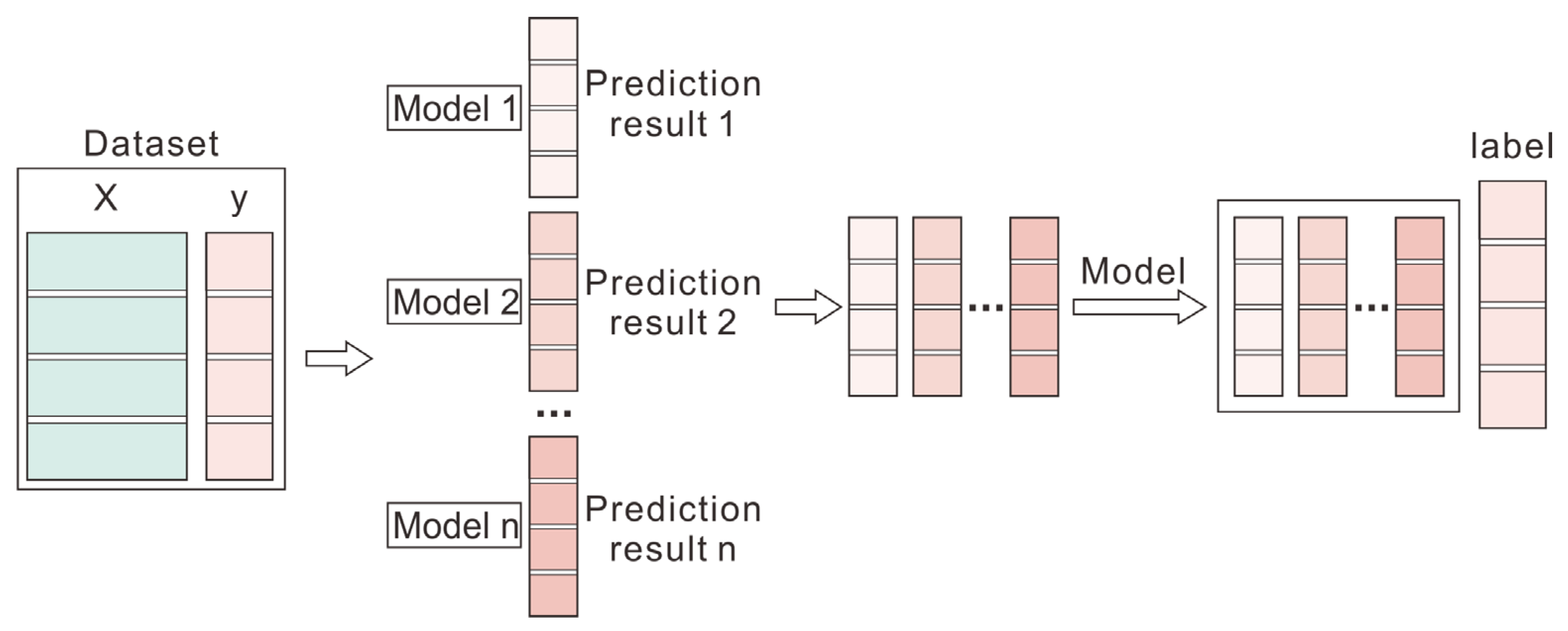
The stacking algorithm is an ensemble learning method that combines the predictions of multiple base learners using a higher-level meta-learner. By integrating the outputs of several models, the meta-learner can achieve better predictive performance and lower generalization error than any individual model (Figure 2). The core principle of stacking is to exploit the complementary strengths of different algorithms. Through multi-level learning, the model captures more complex patterns and has improved prediction accuracy.
The algorithm consists of three main steps. First, multiple base learners (e.g., decision trees, support vector machines, and neural networks) are trained, expressed as
h1, h2, …, hn
Second, the predictions of these base learners on the training dataset are combined to construct a new feature matrix, which, together with the original labels, forms a secondary training dataset. Finally, a meta-learner (e.g., linear or logistic regression) is trained on this dataset. The stacking model can be expressed as
H(X) = F(h1(X), h2(X), …, hk(X))
where H is the final prediction, F is the meta-learner function, and X represents the input feature vector.

3.2. Base Learners

3.2.1. Random Forest (RF)

The Random Forest (RF) algorithm, proposed by Leo Breiman in 2001 [30], is an ensemble learning method that combines multiple decision trees to improve predictive performance. In this study, RF was used as a regression model for predicting continuous elemental concentrations. The model constructs multiple decision trees using bootstrap samples drawn from the training dataset, while random subsets of input features are selected at each node split. For regression tasks, each tree produces a continuous prediction, and the final RF output is obtained by averaging the predictions of all trees. This ensemble strategy reduces variance, improves robustness to noise, and mitigates overfitting.
The decision trees in RF are typically constructed using the CART algorithm [30]. Unlike classification trees, which rely on impurity measures such as the Gini index, CART regression trees select the optimal splits by minimizing prediction error or variance within the resulting child nodes. In this study, the split criterion is defined using the mean squared error [31]:
M S E ( T ) = 1 n i = 1 n ( y i y ¯ ) 2
where T represents the sample set at a given node, n is the number of samples in T , yi is the target elemental concentration of the i-th sample, and y ¯ is the mean target value of all samples in T. Lower MSE indicates reduced within-node variance and better partitioning performance.
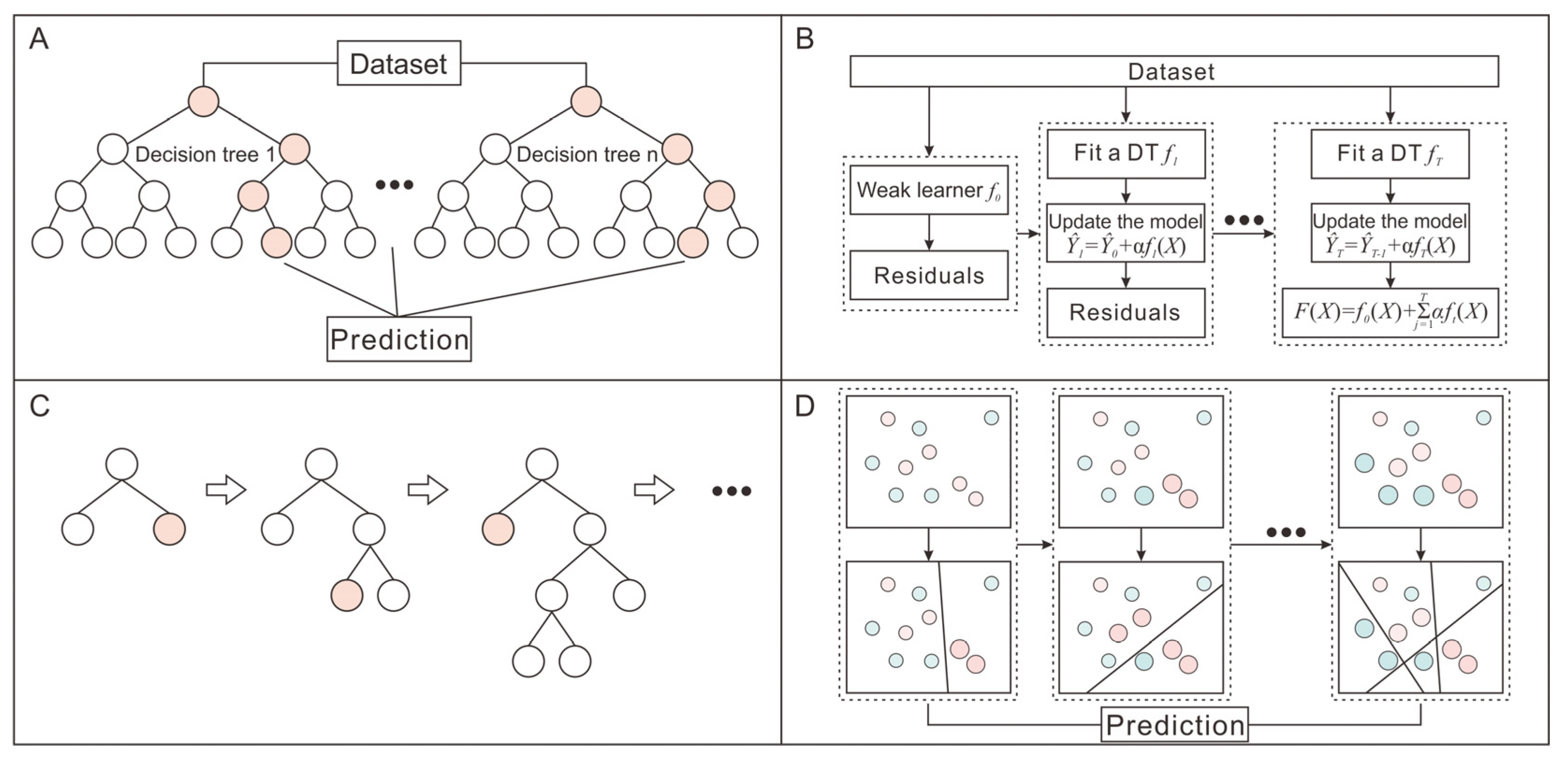
Based on this criterion, multiple regression trees are constructed, and their outputs are averaged to generate the final prediction. During the training, bootstrap sampling and random feature selection increase diversity among trees. This dual-randomization strategy enhances model generalization and improves stability for nonlinear log–element prediction tasks (Figure 3A).

3.2.2. XGBoost

The XGBoost algorithm, proposed by Chen and Guestrin (2016), is an ensemble learning method based on the gradient boosting framework [32]. It sequentially constructs decision trees, with each tree learning the residuals between the predictions of previous trees and the true values. The objective function is optimized using a second-order Taylor expansion with regularization, enabling multiple weak learners to be integrated into a strong predictive model.
During training, XGBoost employs two optimization strategies: (i) an exact greedy algorithm to determine optimal split points and (ii) a weighted quantile sketch algorithm to efficiently process large-scale datasets (Figure 3B). As a result, the method provides high prediction accuracy, robustness to missing data, resistance to overfitting, and efficient parallel computation.
The base learners in XGBoost are CART regression trees. Following Chen and Guestrin [32], the objective function consists of a loss term and a regularization term and is approximated using a second-order Taylor expansion:
Obj = ∑N i=1[gifm (xi) + 1/2 × (hif2 m(xi)] + γT + 1/2 × λ∑T j=1wj2
where g i and h i are the first-order and second-order gradients of the loss function, f m is the m-th tree, T is the number of leaf nodes, w j is the weight of the j-th leaf node, and γ and λ are regularization parameters.

3.2.3. LightGBM

The LightGBM, proposed by Microsoft Research Asia in 2017 [33], is an ensemble learning algorithm based on the gradient boosting framework. Similar to other gradient boosting methods, it sequentially constructs decision trees, with each tree fitting the residuals of previous predictions. Through iterative residual fitting, prediction errors are progressively reduced, allowing multiple weak learners to form a strong predictive model. LightGBM is characterized by fast training speed, low memory consumption, high prediction accuracy, and efficient handling of high-dimensional datasets.
LightGBM adopts a histogram-based algorithm with several additional optimizations. Unlike the level-wise growth strategy used in conventional GBDT implementations, it applies a leaf-wise growth strategy with depth constraints to improve both efficiency and prediction accuracy (Figure 3C) [33]. The split optimization process is expressed as
(pm, fm, vm) = arg min(p,f,v)L(Tm−1 (X).split(p,f,v),Y)
where p m , f m and v m are the split position, split feature, and split threshold, respectively. T m 1 is the decision tree model after the ( m 1 )-th iteration. L is the loss function.

3.2.4. CatBoost

CatBoost is a gradient boosting algorithm with strong capabilities for handling categorical features [34]. It is based on the standard gradient boosting framework, in which multiple regression trees are sequentially constructed to minimize prediction errors. CatBoost differs from conventional boosting methods through the use of ordered boosting and ordered target statistics, which reduce prediction shift and target leakage during training. In addition, it incorporates efficient techniques for handling categorical variables directly without extensive preprocessing (Figure 3D). Consequently, CatBoost achieves high prediction accuracy, requires minimal feature preprocessing and shows relatively low sensitivity to hyperparameter settings.
During tree construction, CatBoost employs a greedy optimization strategy similar to that of XGBoost, to determine optimal split points ( f m , v m ) . For categorical variables, split gains are calculated using statistically encoded target representations. Following the CatBoost framework proposed by Prokhorenkova et al. [34], the final model is expressed as a weighted combination of all trees:
F M ( x ) = m = 1 M η f m ( x )
where F M ( x ) is the final CatBoost prediction, M is the number of boosting iterations, η is the learning rate, and f m ( x ) is the regression tree fitted during the m-th iteration.

4. Formation Element Prediction Model

All model construction, training, validation, and prediction workflows in this study were implemented in Python (version 3.11).

4.1. Data Preprocessing

The dataset used in this study was collected from wells J404, J32, and J34 in the Jiqing Oilfield, located in the Junggar Basin. After depth matching and preprocessing, 115,668 depth-aligned samples were retained for model construction and validation. The dataset includes 11 conventional logging curves: acoustic transit time (AC), azimuth (AZIM), compensated neutron log (CNL), bulk density (DEN), deviation angle (DEVI), natural gamma ray (GR), point resistivity (RI), true resistivity (RT), flushed zone resistivity (RXO), spontaneous potential (SP), and total porosity (ZTCMR). ECS-derived elemental measurements include aluminum (Al), calcium (Ca), iron (Fe), silicon (Si), sulfur (S), and gadolinium (Gd). However, S values are close to zero for most samples, and Gd shows extremely low concentrations with limited variability. Therefore, S and Gd were treated as auxiliary ECS measurements and excluded from the final prediction targets. The final prediction targets were Al, Ca, Fe, and Si.
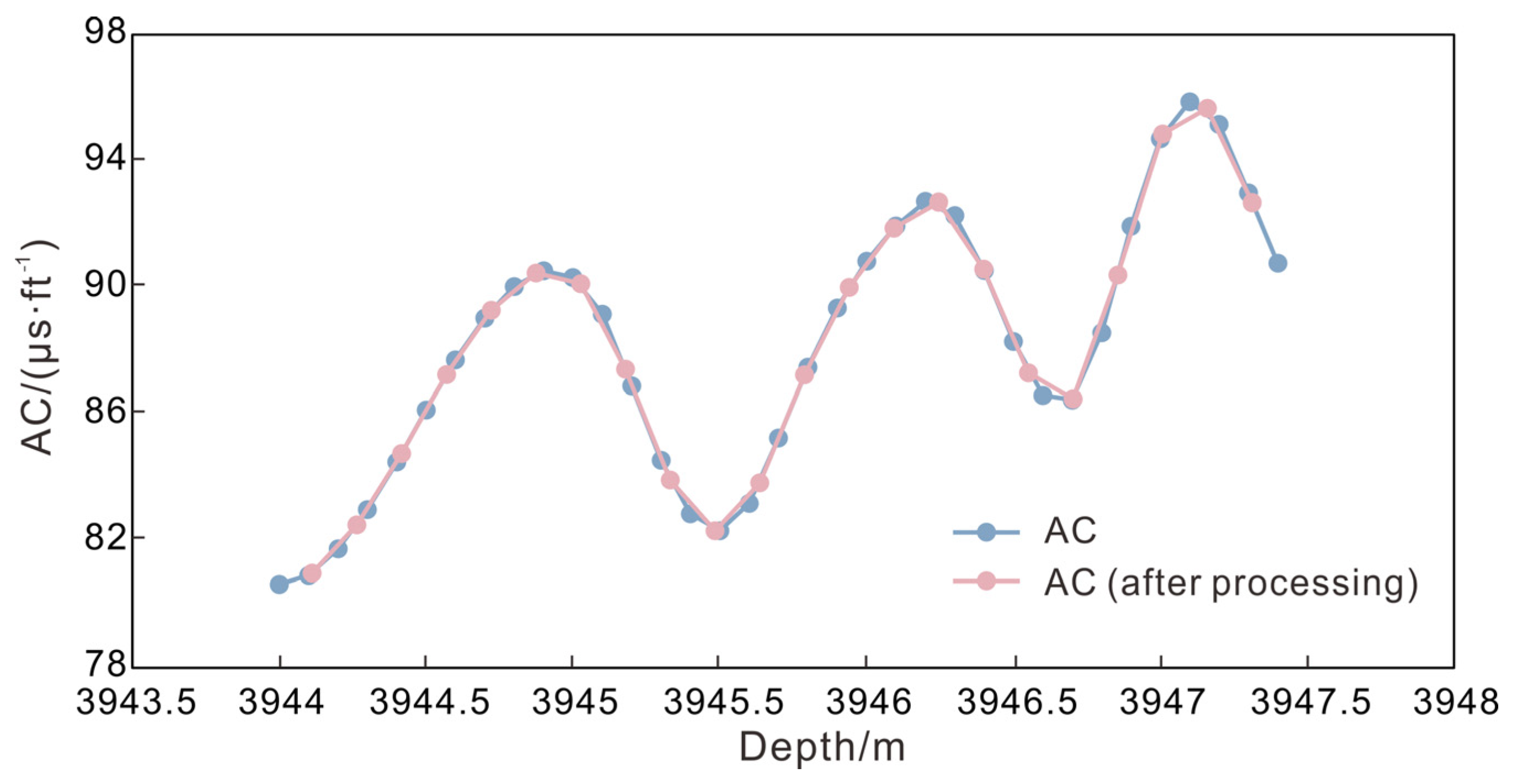
The ECS depth data were used as the reference framework, and cubic spline interpolation [35] was applied to depth-match the conventional logging curves. Figure 4 compares a portion of the AC log before and after resampling, showing that the processed data preserved the overall trend of the original measurements.
The Mahalanobis distance [36] was then used to identify and remove the top 5% of outliers. After outlier filtering, 109,884 valid samples remained for model construction and validation. The Mahalanobis distance measures the distance between a sample and the multivariate data distribution while accounting for correlations and variance structure. It is defined as
MD(x) = sqrt[(xμ)T−1(xμ)]
where μ is the mean vector and Σ 1 is the inverse of the covariance matrix.
Model validation was conducted using randomly shuffled five-fold cross-validation. Before splitting, samples from the three wells were pooled and randomly shuffled. In each fold, four subsets were used for training and the remaining subset for validation. This procedure was repeated five times so that each subset served once as the set, and the final model performance was obtained by averaging the validation results across the five folds.
To avoid data leakage, all data-driven preprocessing and model-development procedures were embedded within a cross-validation workflow. In each fold, correlation-based feature selection, Z-score normalization, hyperparameter tuning, and model training were performed exclusively on the training subset. The validation subset was not used for feature selection correlations, normalization parameter estimation, hyperparameter optimization, or model fitting. The preprocessing parameters and selected features derived from the training subset were then applied to the corresponding validation subset. Deterministic feature-engineering operations, including squared terms, logarithmic transformations, and interaction features, were consistently applied to both training and validation subsets after data splitting.

4.2. Feature Engineering and Data Normalization

Feature engineering aims to construct more informative nonlinear and interaction features from the original variables, enabling the model to better capture complex relationships. To improve model learning and generalization, three feature-enhancement techniques were applied: squared terms, logarithmic transformations, and interaction features. These operations are deterministic transformations and were applied consistently to both the training and validation subsets within each cross-validation fold.
Data normalization was performed to standardize feature scales and prevent variables with larger magnitudes from dominating model training. To avoid data leakage, Z-score standardization [37] was implemented independently within each cross-validation fold. Specifically, the mean and standard deviation were calculated using only the training subset, and the same normalization parameters were then applied to the corresponding validation subset. The validation data were not used to estimate normalization parameters. The Z-score transformation, or “standardized score”, is expressed as
x* = (xμ)/σ
where x * is the normalized value, μ is the mean, and σ is the standard deviation of the feature in the training dataset.

4.3. Model Evaluation Metrics

The predictive performance of the regression models was evaluated using five commonly used metrics: mean absolute error (MAE), mean squared error (MSE), root mean square error (RMSE), coefficient of determination (R2), and mean absolute percentage error (MAPE) [31,38,39]. MAE, MSE, and RMSE quantify the absolute and squared deviations between predicted and measured values, R2 measures the proportion of variance explained by the model, and MAPE evaluates the relative prediction error. These metrics are defined as follows:
M A E = 1 n i = 1 n | y i y ^ i |
M S E = 1 n i = 1 n ( y i y ^ i ) 2
R M S E = 1 n i = 1 n ( y i y ^ i ) 2
R 2 = 1 i = 1 n ( y i y ^ i ) 2 i = 1 n ( y i y ¯ ) 2 = 1 M S E σ 2
M A P E = 100 % n i = 1 n | y i y ^ i y i |
where y i is the true value of the i -th sample, y ^ i is the predicted value of the i -th sample, y ¯ and σ 2 are the mean and variance of the true values, respectively, and n is the total number of samples. It should be noted that MAPE is not applicable when the measured values contain zeros, because the denominator in the percentage error becomes undefined.

4.4. Model Hyperparameter Selection

Hyperparameter tuning is essential for improving the performance and generalization capability of machine learning models. By optimizing parameter combinations, model accuracy can be enhanced while reducing the risk of overfitting.
In this study, the Optuna optimization algorithm was used to tune the hyperparameters of the individual models, whereas linear regression was adopted as the meta-learner in the stacking framework. The optimal hyperparameter settings are summarized in Table 1.

5. Evaluation and Application of the Stacking Ensemble Model for Formation Element Prediction

5.1. Model Evaluation

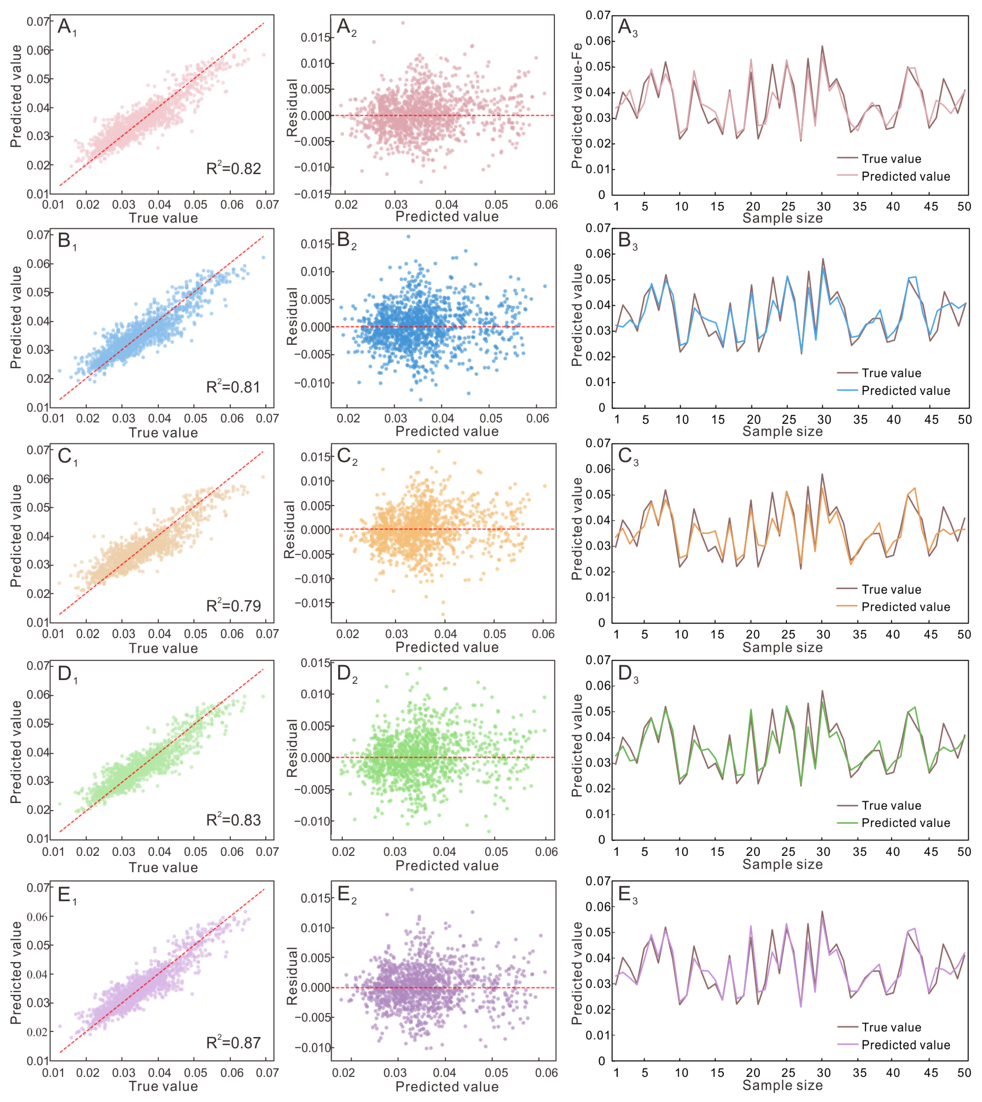
To comprehensively evaluate model performance, four classical machine learning models—Random Forest, XGBoost, LightGBM, and CatBoost—were first developed as base regressors. A stacking ensemble strategy was then applied to build the meta-learner. Fe was selected as the representative target element for comparing model performance, as shown in Figure 5. All models achieved satisfactory prediction accuracy, with R2 values close to 0.8. Among them, the stacking ensemble model produced the highest R2 value for Fe prediction, while its performance stability across different target elements and cross-validation folds is further evaluated in Table 2.
Specifically, for Fe prediction, CatBoost, LightGBM, Random Forest, and XGBoost achieved R2 values of 0.82, 0.81, 0.79, and 0.83, respectively (Figure 5A1–D1). The stacking ensemble model achieved the highest R2 value of 0.87 (Figure 5E1). Across different elemental predictions, Random Forest generally showed lower performance, whereas XGBoost, LightGBM, and CatBoost produced comparable results, with variations depending on the target element. Despite its relatively weaker performance, Random Forest remains a valuable benchmark because of its inherent parallel training capability and resistance to overfitting. These results highlight the advantage of gradient boosting algorithms in capturing complex nonlinear relationships through iterative error correction.
Residual analysis further reveals differences among the models. As shown in Figure 5C2, Random Forest exhibits the widest residual distribution and exhibits slight systematic bias in some prediction intervals, suggesting limited ability to fully capture complex data patterns. In contrast, the gradient boosting models show more concentrated and homogeneous residual distributions. Among them, LightGBM shows a residual mean closest to zero, indicating its superior bias correction capability. Comparisons between predicted and measured values on the validation dataset (Figure 5A3–E3) show generally good agreement, with predicted curves closely matching the true values and effectively reproducing peak variations.
The stacking ensemble model successfully integrates the strengths of the individual models. As shown in Figure 5E1, it produces the most compact and concentrated scatter distribution, without obvious prediction bias or saturation effects in either high- or low-value regions. The residual distribution (Figure 5E2) also exhibits the most favorable characteristics among all models. The ensemble model achieved the highest coefficient of determination (R2 = 0.87) and the lowest root mean square error (RMSE = 0.0031). These results demonstrate that ensemble learning, effectively reduces the bias and variance associated with individual models, thereby improving generalization capability and prediction robustness. Consequently, the stacking ensemble model represents the optimal solution for the prediction task considered in this study.
Based on the target-element selection described in Section 4.1, model performance was evaluated for four major ECS-derived elements: Al, Ca, Fe, and Si. S and Gd were treated as auxiliary ECS measurements rather than final prediction targets because their concentrations were extremely low or close to zero in most samples, resulting in limited statistical variability and low predictive significance. Separate models were trained for each target element, and the stacking ensemble framework was used to generate the final elemental predictions. To provide a clearer statistical interpretation, Table 2 reports the number of valid samples for each element and summarizes model performance as the mean ± standard deviation across the five cross-validation folds. A multiple linear regression model was included as a baseline using the same input features and validation strategy, enabling direct comparison between the stacked ensemble approach and a conventional linear log–element prediction method.
These results indicate that the stacking ensemble model can integrate complementary information from individual learners and partially reduce model-specific bias. Compared with the individual tree-based models, the stacked ensemble achieved higher prediction accuracy for Fe in the present validation dataset. Therefore, it was selected as the final model for subsequent elemental prediction. Its performance across different target elements is further evaluated using the cross-validation statistics summarized in Table 2.

5.2. Hydraulic-Fracturing Parameter Analysis Based on Model Predictions

Using well JHW87-11 as an example, the proposed model was applied to predict formation elemental compositions. The predicted results were integrated with pressure and logging data to analyze relationships among elemental composition, logging responses, and hydraulic-fracturing pressure. The predicted elemental compositions were not interpreted as direct controls of fracture pressure, but rather as lithological indicators reflecting variations in mineral composition, rock fabric, brittleness, and elastic properties.
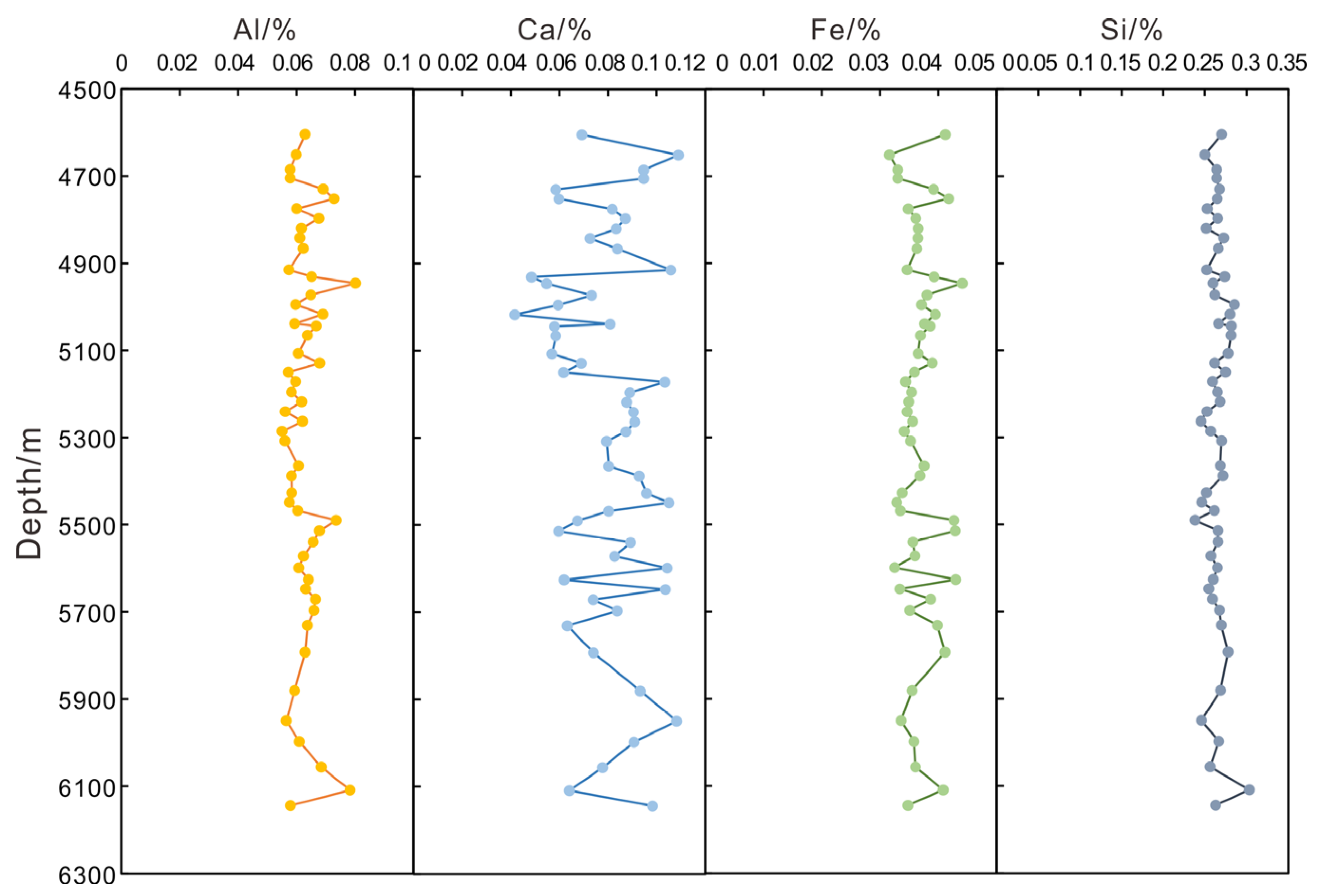
A total of 32 fracturing stages were completed in well JHW87-11, subdivided into 52 operational intervals. The midpoint depth of each stage was selected, and the average logging values within each interval were used as input features. The predicted elemental compositions are shown in Figure 6.
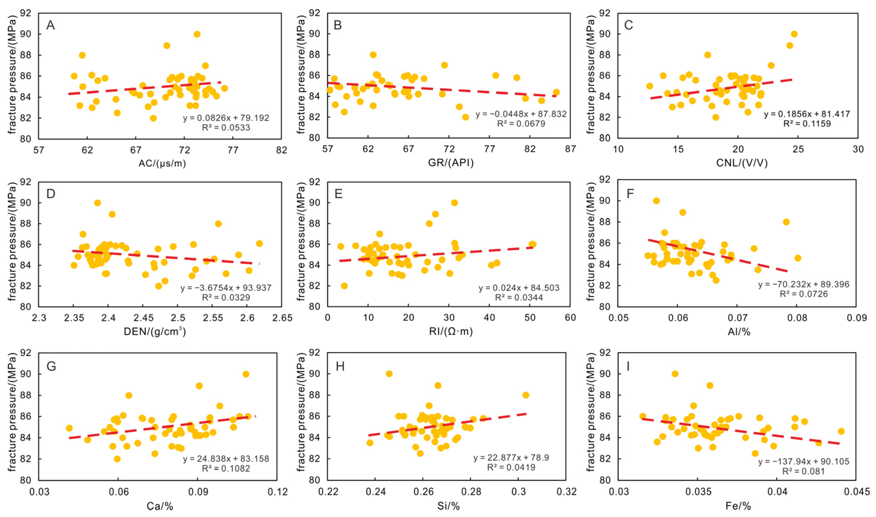
Using the predicted elemental compositions and logging parameters as independent variables, and fracture pressure as the dependent variable, bivariate scatter plots were constructed to evaluate the relationships among these parameters.
As shown in Figure 7, fracture pressure exhibits generally weak overall correlations with both elemental compositions and conventional logging parameters, although localized sensitivities are observed. This suggests that the relationship between elemental composition and fracture pressure should not be interpreted as a simple linear or direct causal relationship. Instead, fracture pressure reflects a coupled field geomechanical response controlled by lithology, mechanical properties, in situ stress conditions, near-wellbore effects, and operational parameters. For elemental composition such as Al, Ca, and Si (Figure 7F–I), fracture pressure does not display a clear linear or monotonic trend. Nevertheless, several important tendencies can be identified. Higher Al content, commonly associated with clay-rich intervals, generally corresponds to lower fracture pressure. This trend suggests that clay-rich rocks may exhibit weaker mechanical strength and more ductile behavior, although the relationship remains scattered and should be regarded as a lithological constraint rather than a direct predictor of fracture pressure. In contrast, Ca, which is commonly associated with carbonate minerals, tends to correspond to slightly higher fracture pressures within the medium-to-high pressure range. This likely reflects the stronger mechanical integrity of carbonate-rich intervals, which require higher stress for fracture initiation. Similar tendencies are also observed for Fe and Si. Higher Si content locally correlates with increased fracture pressure, possibly because siliceous components enhance rock stiffness and brittleness. However, the response of Fe is less consistent, indicating that Fe-bearing minerals may originate from multiple mineralogical sources with different mechanical implications. As Ca- and Si-rich brittle components increase, the variability in fracture pressure also becomes more pronounced.
Among the conventional logging parameters, DEN exhibits the clearest relationship with fracture pressure (Figure 7D), showing a distinct positive correlation. Higher density generally indicates more compact and well-cemented rocks, which may require higher fracture pressure. In contrast, AC displays an inverse relationship with fracture pressure (Figure 7A): lower AC values correspond to higher acoustic velocities and stronger lithologies, which are also associated with higher fracture pressure. These responses are consistent with the mechanical interpretation that more compact intervals generally exhibit greater elastic stiffness and stronger resistance to fracture initiation. CNL shows a weak negative correlation with fracture pressure (Figure 7C), suggesting that higher-porosity and mechanically weaker intervals are more susceptible to fracturing and may require lower initiation pressure. Moreover, the dispersion of the data indicates that porosity effects are not independent, but instead interact with lithology, cementation, stress conditions, and operational parameters.
The responses of GR and RI further highlight the dual lithological and mechanical controls of fracture pressure (Figure 7B,E). High GR values, commonly associated with clay-rich intervals, correspond to lower fracture pressure, reflecting weaker mechanical resistance. In contrast, intervals with high RI values, indicative of stronger compaction and lower fluid conductivity, tend to exhibit higher fracture pressure, suggesting greater structural integrity and higher energy requirements for fracture initiation. Therefore, the observed trends of “high clay–low fracture pressure” and “high compaction–high fracture pressure” provide useful lithological and mechanical constraints for pressure response interpretation, although they should not be considered deterministic rules for fracturing design.
Overall, fracture pressure in the study area reflects coupled controls between lithological composition, pore structure, mechanical properties, and in situ stress conditions:
  • High clay content (indicated by Al and GR) → weaker mechanical resistance → lower fracture pressure;
  • High Ca- and Si-related components (indicated by Ca, Si, and RI) → stronger rock fabric and greater brittleness → locally higher fracture-initiation resistance;
  • Mechanical-sensitive parameters, such as density (DEN) and acoustic transit time (AC), provide logging-derived constraints for interpreting fracture-pressure variations.
These results demonstrate that elemental compositions predicted from conventional logging data can provide supplementary lithological constraints for interpreting hydraulic-fracturing pressure responses. However, the present analysis is based on a single example well and post hoc interval-scale comparisons. Therefore, the observed relationships should be regarded as interpretative indicators rather than direct optimization criteria for fracturing design. Their applicability to other wells and reservoirs requires further stress calibration, independent validation, and integration with field-scale stimulation-response data.
To avoid a purely correlation-based interpretation, an element-based brittleness proxy was further introduced to establish a lithological link between predicted elemental compositions and pressure-related responses:
B I e = S i + C a S i + C a + A l + F e
where B I e represents the element-based brittleness proxy. Si and Ca are used to represent siliceous- and carbonate-related brittle components, whereas Al mainly reflects clay-rich components. Fe is included in the denominator because of its uncertain mechanical significance. Therefore, B I e should be regarded as a lithological indicator of brittleness tendency rather than a direct geomechanical brittleness index.
To further constrain the mechanical interpretation, logging-derived dynamic elastic parameters were incorporated. Because shear-wave slowness and laboratory mechanical test data were unavailable, dynamic Young’s modulus ( E d ) [40,41] and dynamic Poisson’s ratio were estimated from conventional logging data and used only as relative mechanical indicators rather than calibrated static rock mechanical properties. Instantaneous shut-in pressure (ISIP) was also used as a first-order pressure constraint. By comparing B I e , E d , ISIP, and measured fracture pressure along well JHW87-11, the elemental–pressure relationship was interpreted through a pathway linking elemental composition, lithological brittleness, dynamic elastic response, and pressure-related fracturing behavior.
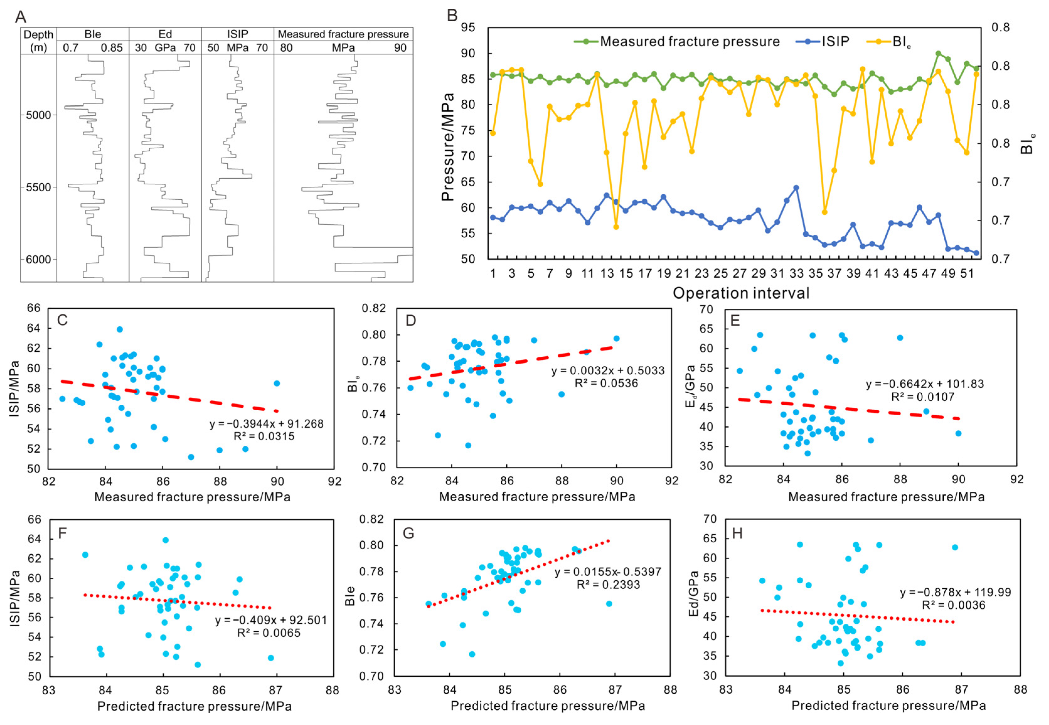
As shown in Figure 8A, B I e , E d , ISIP, and measured fracture pressure all vary significantly along the well, indicating that fracture-pressure response cannot be explained solely by elemental composition. Figure 8B further demonstrates that measured fracture pressure is consistently higher than ISIP and does not strictly follow the B I e trend. From a porous-media perspective, this response is also influenced by pressure transmission and hydraulic resistance within connected pore-throat networks. Mohammadizadeh et al. [42] described porous media as networks of pores and connecting throats, showing that fluid flow is controlled by pore connectivity, local head loss, roughness-related resistance, and flow-regime transition. Therefore, the interval-scale pressure variations observed in well JHW87-11 likely reflect coupled effects of lithological composition, dynamic mechanical properties, pore-network-controlled pressure transmission, in situ stress conditions, near-wellbore effects, and operational parameters. Figure 8C–H are cross-plots between measured fracture pressure, predicted fracture pressure, and the parameters   B I e , E d , and ISIP. These plots show the covariation trends and statistical relationships among these variables.
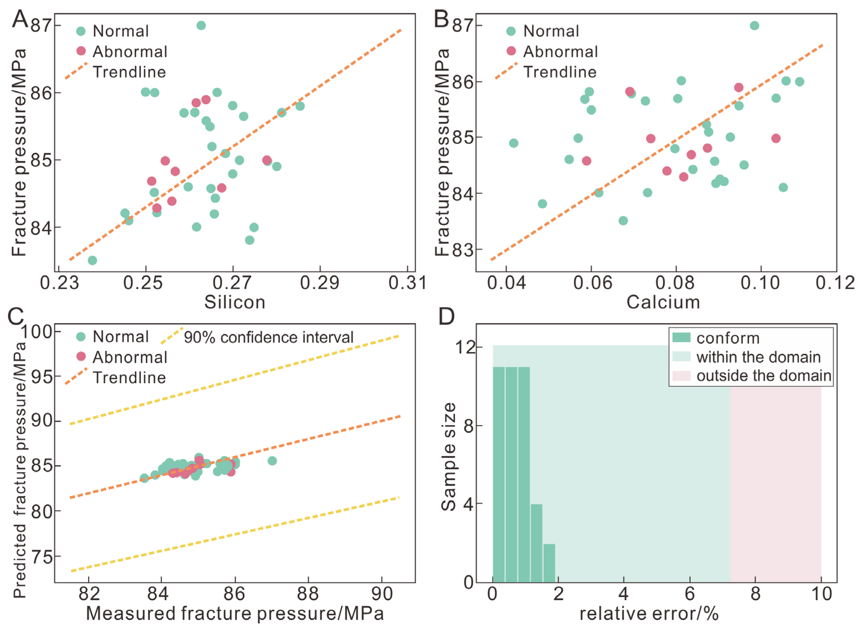
As shown in Figure 9, cross-plots between predicted elemental compositions and hydraulic-fracturing response (fracture pressure) were constructed for well JHW87-11. The empirical regression equations are provided in Appendix A because they represent model expressions rather than direct study results. In the main text, the cross-plots are used only to illustrate statistical associations and not to establish a generalized fracture-pressure prediction equation.
The cross-plot analysis shows a post hoc conformity rate of 93.6% (44/47 samples), with an RMSE of 0.627 MPa. Si and Ca exhibit locally positive correlations with fracture pressure, suggesting that siliceous- and carbonate-related components may provide useful lithological constraints for interpreting pressure responses. However, these results should not be considered as independent validation of a generalized fracture-pressure prediction model. Therefore, the proposed workflow should be used as an exploratory interpretation framework rather than a deterministic tool for hydraulic-fracturing optimization or operational-risk prediction.

6. Discussion

6.1. Geological Significance of Conventional-Log-Driven Elemental Characterization

Continuous characterization of formation elemental composition is important for evaluating mixed fine-grained shale oil reservoirs because elemental variations provide direct constraints on mineralogical composition, lithofacies heterogeneity, sedimentary differentiation, mechanical properties, and fracability. In saline lacustrine shale oil systems, such as the Jimusar Sag, rapid lithological transitions and mixed sedimentation commonly generate strong vertical and lateral heterogeneity. Under these conditions, discrete core measurements or sparsely distributed ECS logs may not be sufficient to characterize the continuous elemental variability of the reservoir. Therefore, establishing reliable relationships between conventional logging responses and ECS-derived elemental concentrations provides a practical approach for extending limited elemental information into uncored or non-ECS intervals.
The workflow proposed in this study is based on the premise that conventional logs contain integrated physical responses related to mineral composition, pore structure, fluid properties, and organic–inorganic associations. Although these responses are indirect and inherently non-unique, they can still preserve meaningful information related to elemental enrichment or depletion when interpreted within an appropriate geological framework. Variations in Fe, Si, Ca, and Al, for example, are closely linked to changes in clay minerals, siliceous components, carbonate minerals, and heavy minerals, which can influence density, natural gamma ray, acoustic, and resistivity responses. Consequently, the prediction task should not be regarded as a purely mathematical regression problem, but rather as a process of extracting geologically meaningful elemental signals from multiple conventional logging curves. In this context, the stacking ensemble framework acts as a data-integration strategy that combines complementary nonlinear responses among conventional logging variables, rather than merely representing an alternative machine learning algorithm.
This interpretation is consistent with the broader concept that data-driven reservoir characterization should be guided by reservoir-specific geological problems rather than by algorithm selection alone. Gavidia et al. [18] demonstrated that, in vuggy carbonate reservoirs, the integration of fit-for-purpose static and dynamic datasets improves continuous permeability modeling and identification of super-K zones. In the present study, the geological objective is different: the main challenge is to obtain continuous elemental information in a heterogeneous saline lacustrine shale oil reservoir where ECS logging is expensive and spatially limited. Accordingly, conventional logging curves and ECS-derived elemental concentrations were paired at the well scale to establish a data foundation for learning log–element relationships within this specific depositional and reservoir framework.
The predicted elemental profiles also have potential engineering significance. Elemental composition is closely related to mineral assemblages, mechanical properties, and fracturing behavior. By linking predicted elemental compositions with hydraulic-fracturing response parameters, this study further evaluates whether the generated elemental profiles can provide useful constraints for fracturing design and abnormal-risk identification. The 93.6% conformity rate between predicted elemental indicators and fracturing-operation status suggests that conventional-log-driven elemental prediction is not only statistically feasible, but also potentially relevant for reservoir engineering applications. Therefore, the main value of the proposed workflow lies in bridging sparse elemental measurements and continuous reservoir characterization in strongly heterogeneous lacustrine shale oil reservoirs.

6.2. Engineering Implications and Limitations of Pressure-Response Interpretation

Hydraulic-fracturing pressure responses have been interpreted from multiple perspectives in previous studies [43]. In the Jimusar shale oil reservoir, fracture development has been linked to lithology, mineral composition, fracture filling, and regional tectonic setting, indicating that fracture behavior is controlled by multiple geological factors [44]. Experimental studies on unconventional reservoir rocks further demonstrate that reservoir heterogeneity and geostress differences can significantly affect hydraulic-fracture initiation, propagation, and spatial distribution [45]. Rock brittleness is commonly used to evaluate fracability, although actual fracture propagation and pressure response are also influenced by bedding, pre-existing interfaces, local stress conditions, and anisotropic mechanical properties [46]. In addition, the discrepancy between dynamic and static Young’s moduli is well recognized, implying that log-derived dynamic elastic parameters should be applied cautiously in the absence of laboratory calibration. From a porous-media perspective, pressure transmission and hydraulic resistance within connected pore-throat networks may further influence pressure behavior during fluid flow [47].
In the present study, the relationship between predicted elemental compositions and hydraulic-fracturing pressure response was investigated using well JHW87-11. Compared with previous studies that analyzed fracture development, brittleness, elastic parameters, and porous-media flow separately, this study integrates predicted elemental profiles with conventional logging parameters, dynamic Young’s modulus, ISIP, and measured fracture pressure. This integrated analysis allows the element–pressure relationship to be interpreted within a combined lithological and mechanical framework. However, the predicted elemental compositions should not be considered as direct controls of fracture pressure. Instead, they are better interpreted as lithological indicators reflecting variations in mineral composition, rock fabric, brittleness tendency, and elastic response among operational intervals. In this sense, the predicted elemental compositions are not merely model outputs, but also useful indicators for identifying pressure-response differences between fracturing intervals.
Several consistent tends emerge from the observed element–pressure relationship. Clay-rich intervals characterized by elevated Al and GR values are generally associated with weaker mechanical resistance and relatively lower fracture-pressure responses. In contrast, intervals enriched in Ca, Si, and RI tend to correspond to more compact and brittle rocks with locally higher fracture-initiation resistance. Density and acoustic transit time further reflect differences in dynamic mechanical behavior. These observations suggest that elemental compositions can provide meaningful constraints on fracture-pressure variations, especially when integrated with conventional logging responses and pressure-related indicators.
The element-based brittleness proxy further links predicted elemental composition with brittleness tendency. By comparing this proxy with dynamic Young’s modulus, ISIP, and measured fracture pressure, the pressure-response interpretation can be extended from elemental composition to lithological brittleness, dynamic mechanical response, and pressure-related fracturing behavior. From this perspective, the element–pressure relationship should not be interpreted as a simple scatter-plot correlation, but rather as a coupled response pattern controlled by interactions among lithology, mechanical properties, and pressure-related conditions. This interpretation also helps explain why intervals with similar elemental trends may nevertheless exhibit different fracturing pressure responses [48].
The present interpretation remains limited to the current well-scale dataset and requires further validation before broader application. The analysis of well JHW87-11 establishes an initial framework for element–pressure interpretation, but its stability across different wells and operational intervals still requires further evaluation. The logging-derived dynamic elastic parameters and ISIP provide useful constraints, although they remain simplified representations of in situ mechanical and pressure conditions. In addition, the predicted elemental profiles may be sensitive to preprocessing procedures such as depth matching, outlier removal, feature engineering, and data normalization. Therefore, the robustness of the proposed element–pressure interpretation should be tested using alternative preprocessing strategies and independent well datasets.
Future work should focus on multi-well validation using datasets that include conventional logs, predicted elemental profiles, ISIP, and hydraulic-fracturing response data. Such analyses would help determine whether the element–pressure relationships identified in this study can be transferable to a broader range of wells and intervals, thereby providing a stronger basis for applying conventional-log-driven elemental prediction to fracturing-response interpretation.

7. Conclusions

This study developed a conventional-log-driven workflow for predicting ECS-derived formation elemental compositions in the Jimusar shale oil reservoir, which is characterized by saline lacustrine mixed sedimentation and strong reservoir heterogeneity. Based on three wells and 109,884 valid samples retained after preprocessing, four major ECS-derived elements—Al, Ca, Fe, and Si—were selected as prediction targets. S and Gd were treated as auxiliary ECS measurements because their concentrations were close to zero or extremely low in most samples. The main conclusions are as follows:
(1)
Conventional logging curves contain useful information for predicting major ECS-derived elemental compositions in the Jimusar shale oil reservoir. The stacked ensemble model achieved stable prediction performance during five-fold cross-validation and outperformed both the multiple linear regression baseline and the individual tree-based models. For Fe prediction, the stacking ensemble achieved the highest validation accuracy, with an R2 value of 0.87.
(2)
Prediction accuracy varied among different elements. Fe showed the highest prediction performance, likely because Fe-bearing clay minerals and heavy minerals strongly influence conventional logging responses such as density, natural gamma ray, acoustic, and resistivity logs. These results indicate that the proposed workflow can capture geologically meaningful log–element relationships, although the strength of these relationships depends on the association between elemental composition, mineral assemblages, and logging responses.
(3)
Cross-plot analysis between predicted elemental compositions and hydraulic-fracturing response parameters yielded a 93.6% conformity rate with operational status. This suggests that the predicted elemental profiles may provide useful auxiliary constraints for fracture-response interpretation and abnormal-risk identification. However, these relationships should be regarded as exploratory statistical associations rather than direct operational guidance, and additional field validation is required before applying the workflow to fracturing-parameter optimization in similar reservoirs.
Overall, this study demonstrates the feasibility of using conventional logging data to predict major ECS-derived elemental compositions in the Jimusar shale oil reservoir. The proposed workflow provides a potentially low-cost approach for continuous elemental characterization where ECS logging is sparse or unavailable. Nevertheless, its operational applicability and generalizability to other wells, stratigraphic intervals, and lacustrine shale oil systems still require further validation using independent field datasets.

Author Contributions

Conceptualization, X.X., J.Z. and D.Y.; methodology, Y.S. (Yue Shen) and S.N.; software, Y.S. (Yue Shen); validation, J.Z., D.Y. and M.H.; writing—original draft preparation, Y.S. (Yue Shen) and S.N.; writing—review and editing, Y.S. (Yinghao Shen); supervision, Y.S. (Yue Shen) and S.N. All authors have read and agreed to the published version of the manuscript.

Funding

This research was funded by National Science and Technology Major Project of the Ministry of Science and Technology of China, grant number 2025ZD1405; And the APC was funded by the National Science and Technology Major Project of the Ministry of Science and Technology of China.

Institutional Review Board Statement

Not applicable.

Informed Consent Statement

Not applicable.

Data Availability Statement

The datasets presented in this study are not publicly available due to confidentiality restrictions associated with oilfield production and operational data. Requests regarding data access should be directed to the corresponding author.

Acknowledgments

The authors have reviewed and edited the output and take full responsibility for the content of this publication.

Conflicts of Interest

Authors Xiaofan Xie, Jinfeng Zhang and Dongji Yang were employed by the company Jiqing Operation Area of Xinjiang Oilfield Company, PetroChina. The remaining authors declare that the research was conducted in the absence of any commercial or financial relationships that could be construed as a potential conflict of interest.

Appendix A

The empirical regression relationship between predicted elemental compositions and measured fracture pressure was used only for post hoc cross-plot comparison:
P f = 67.23 ± 18.48 + 17.28 ± 103.52 A l + 45.01 ± 43.86 C a + 110.21 ± 258.19 F e + 42.41 ± 43.19 S i R 2 = 0.374 ,   R M S E = 0.627   MPa
where P f is the measured fracture pressure. A l , C a , F e , and S i represent the predicted elemental compositions.

References

  1. Jia, C.; Zheng, M.; Zhang, Y. Unconventional hydrocarbon resources in China and the prospect of exploration and development. Pet. Explor. Dev. 2012, 39, 139–146. [Google Scholar] [CrossRef]
  2. Li, G.; Zhu, R. Progress, challenges and key issues of unconventional oil and gas development of CNPC. China Pet. Explor. 2020, 25, 1–13. [Google Scholar] [CrossRef]
  3. Zou, C.; Yang, Z.; Zhang, G.; Zhu, R.; Tao, S.; Yuan, X.; Hou, L.; Dong, D.; Gou, Q.; Song, Y.; et al. Theory, technology and practice of unconventional petroleum geology. Earth Sci. 2023, 34, 951–965. [Google Scholar] [CrossRef]
  4. Huang, J.; Zhang, Z.; Yang, Z.; Huang, Y.; Di, J.; Zhang, L. Quantitative prediction of mineral component content and brittleness index in tight rocks based on multivariate regression analysis. Xinjiang Pet. Geol. 2016, 37, 346–351. [Google Scholar]
  5. Zhao, J.; Zhang, L.; Li, S.; Li, Z.; Niu, Z.; Guo, X. Research on the prediction method of shale clay mineral and quartz content in the Z area of Taihang. Prog. Geophys. 2019, 34, 681–686. [Google Scholar] [CrossRef]
  6. Lawal, A.; Yang, Y.; He, H.; Baisa, N. Machine learning in oil and gas exploration. IEEE Access. 2024, 12, 19035–19058. [Google Scholar] [CrossRef]
  7. Luo, G.; An, X.; Yao, W.; Zou, Y. Application status and development trends of artificial intelligence in logging interpretation for unconventional oil and gas reservoirs. Pet. Sci. Bull. 2025, 10, 908–925. [Google Scholar] [CrossRef]
  8. Xue, C.; McBeck, J.; Lu, H.; Yan, C.; Zhong, J.; Wu, J.; Renard, F. Classification of shale lithofacies with minimal data: Application to the early Permian shales in the Ordos Basin, China. J. Asian Earth Sci. 2024, 259, 105901. [Google Scholar] [CrossRef]
  9. Liu, Y.; Zhu, R.; Zhai, S.; Li, N.; Li, C. Lithofacies identification of shale formation based on mineral content regression using LightGBM algorithm: A case study in the Luzhou block, South Sichuan Basin, China. Energy Sci. Eng. 2023, 11, 4256–4272. [Google Scholar] [CrossRef]
  10. Fu, Z.; Zhang, X.; Yan, Y.; Xu, X.; Zhou, F.; Li, X.; Zhou, Q.; Mai, W. The evolution of machine learning in Large-Scale mineral prospectivity prediction: A decade of innovation. Mineals 2025, 15, 1042. [Google Scholar] [CrossRef]
  11. Shen, Y.; Wu, S.; Shen, Y.; Wu, K.; Li, Y.; Zhang, D.; Xing, H.; Wang, C. Separate classification prediction model for lithofacies identification of paleogene Yingxiongling Shale, Qaidam Basin. Energy Fuels 2025, 39, 7751–7765. [Google Scholar] [CrossRef]
  12. Laalam, A.; Boualam, A.; Ouadi, H.; Djezzar, S.; Tomomewo, O.; Mellal, I.; Bakelli, O.; Merzoug, A.; Chemmakh, A.; Latreche, A.; et al. Application of machine learning for mineralogy prediction from well logs in the Bakken petroleum system. In Proceedings of the SPE Annual Technical Conference and Exhibition, Houston, TX, USA, 3–5 October 2022; p. SPE-210336-MS. [Google Scholar]
  13. Wang, X.; Yu, W.; Ma, X.; Zhou, T.; Tai, H.; Cui, Q.; Deng, K.; Lu, Y.; Liu, Z. Identification and application of shale lithofacies based on conventional logging curves: A case study of the second member of Funing Formation in Qintong Sag, Subei Basin. Pet. Reserv. Eval. Dev. 2024, 14, 699–706. [Google Scholar] [CrossRef]
  14. Zhu, Z.; Guo, J.; Gu, B.; Wang, L.; Wang, S.; Zhang, Z. Multi-mineral fine inversion and prediction methods based on formation elemental logging. Prog. Geophys. 2025, 40, 1045–1059. [Google Scholar] [CrossRef]
  15. Anifowose, F.A.; Labadin, J.; Abdulraheem, A. Ensemble Machine Learning: An Untapped Modeling Paradigm for Petroleum Reservoir Characterization. J. Pet. Sci. Eng. 2017, 151, 480–487. [Google Scholar] [CrossRef]
  16. Li, W.; Zhang, T.; Liu, X.; Dong, Z.; Dong, G.; Qian, S.; Yang, Z.; Zou, L.; Lin, K.; Zhang, T. Machine Learning-Based Fracturing Parameter Optimization for Horizontal Wells in Panke Field Shale Oil. Sci. Rep. 2024, 14, 6046. [Google Scholar] [CrossRef]
  17. Qiao, Y.; Lin, C.; Zhao, Y.; Zhou, L. Integrating Temporal Deep Learning Models for Predicting Screen-Out Risk Levels in Hydraulic Fracturing. Geoenergy Sci. Eng. 2025, 244, 213442. [Google Scholar] [CrossRef]
  18. Gavidia, J.C.R.; Mohammadizadeh, S.; Chinelatto, G.F.; Basso, M.; da Ponte Souza, J.P.; Domínguez Portillo, L.E.; Eltom, H.A.; Vidal, A.C.; Goldstein, R.H. Bridging the Gap: Integrating Static and Dynamic Data for Improved Permeability Modeling and Super K Zone Detection in Vuggy Reservoirs. Geoenergy Sci. Eng. 2024, 241, 213152. [Google Scholar] [CrossRef]
  19. Yang, Z.; Hou, L.; Lin, S.; Luo, X.; Zhang, L.; Wu, S.; Cui, J. Geologic characteristics and exploration potential of tight oil and shale oil in Lucaogou Formation in Jimusar sag. China Pet. Explor. 2018, 23, 76–85. [Google Scholar] [CrossRef]
  20. Xu, L.; Chang, Q.; Yang, C.; Tao, Q.; Wang, S.; Fei, L.; Xu, S. Characteristics and oil-bearing capability of shale oil reservoir in the Permian Lucaogou Formation, Jimusaer sag. Oil Gas Geol. 2019, 3, 535–549. [Google Scholar] [CrossRef]
  21. Zhao, W.; Hu, S.; Hou, L.; Yang, T.; Li, X.; Guo, B.; Yang, Z. Types and resource potential of continental shale oil in China and its boundary with tight oil. Pet. Explor. Dev. 2020, 47, 1–11. [Google Scholar] [CrossRef]
  22. Gong, D.; Song, Y.; Peng, M.; Liu, C.; Wang, R.; Wu, W. The Hydrocarbon Potential of Carboniferous Reservoirs in the Jimsar Sag, Northwest China: Implications for a Giant Volcanic-Petroleum Reserves. Front. Earth Sci. 2022, 10, 879712. [Google Scholar] [CrossRef]
  23. Ge, Y.; Ren, L.; He, Y.; Ma, F.; Wang, Q.; Du, K.; Li, H. Main factors controlling the tight oil enrichment in the 7th oil layer group of the Triassic Yanchang Formation in Fuxian-Ganquan area, Ordos Basin. Oil Gas Geol. 2018, 39, 1190–1200. [Google Scholar] [CrossRef]
  24. Zhang, C.; Zhu, D.; Luo, Q.; Liu, L.; Liu, D.; Yan, L.; Zhang, Y. Major factors controlling fracture development in the Middle Permian Lucaogou Formation tight oil reservoir, Junggar Basin, NW China. J. Asian Earth Sci. 2017, 146, 279–295. [Google Scholar] [CrossRef]
  25. Fang, X.; Wang, Y.; Zhang, Y.; Li, D. Rock Mechanical Properties and Fracability Evaluation of Deep Tight Hybrid Sedimentary Rocks Reservoirs: A Case Study of Lucaogou Formation in Jimsar Sag, Junggar Basin. J. Pet. Explor. Prod. Technol. 2025, 15, 67. [Google Scholar] [CrossRef]
  26. Ding, X.; He, W.; Liu, H.; Guo, X.; Zha, M.; Jiang, Z. Organic matter accumulation in lacustrine shale of the Permian Jimsar Sag, Junggar Basin, NW China. Pet. Sci. 2023, 20, 1324–1346. [Google Scholar] [CrossRef]
  27. Li, J.; Jin, A.; Zhu, R.; Lou, Z.; on behalf of The Hebei Scolike Petroleum Technology Co., Ltd. Micro-occurrence characteristics and charging mechanism in continental shale oil from Lucaogou Formation in the Jimsar Sag, Junggar Basin, NW China. PLoS ONE 2024, 19, e0297104. [Google Scholar] [CrossRef]
  28. Liu, J.; Li, J.; Song, Z.; Shen, A. Flow characteristics of shale oil and their geological controls: A case study of the Lucaogou Formation in the Jimsar Sag, Junggar Basin. Pet. Sci. 2025, 22, 3900–3914. [Google Scholar] [CrossRef]
  29. Zhi, D.; Tang, Y.; Yang, Z.; Guo, X.; Zheng, M.; Wan, M.; Huang, L. Geological characteristics and accumulation mechanism of continental shale oil in Jimusaer sag, Junggar Basin. Oil Gas Geol. 2019, 40, 524–534. [Google Scholar] [CrossRef]
  30. Breiman, L. Random Forests. Mach. Learn. 2001, 45, 5–32. [Google Scholar] [CrossRef]
  31. Chai, T.; Draxler, R.R. Root Mean Square Error (RMSE) or Mean Absolute Error (MAE)? Geosci. Model Dev. 2014, 7, 1247–1250. [Google Scholar] [CrossRef]
  32. Chen, T.; Guestrin, C. XGBoost: A scalable tree boosting system. In Proceedings of the 22nd ACM SIGKDD International Conference on Knowledge Discovery and Data Mining, San Francisco, CA, USA, 13–17 August 2016. [Google Scholar] [CrossRef]
  33. Ke, G.; Meng, Q.; Finley, T.; Wang, T.; Chen, W.; Ma, W.; Ye, Q.; Liu, T. LightGBM: A highly efficient gradient boosting decision tree. In Proceedings of the 31st Conference on Neural Information Processing Systems (NIPS 2017), Long Beach, CA, USA, 4–9 December 2017. [Google Scholar]
  34. Prokhorenkova, L.; Gusev, G.; Vorobev, A.; Dorogush, A.; Gulin, A. CatBoost: Unbiased boosting with categorical features. In Proceedings of the 32nd Conference on Neural Information Processing Systems, Montréal, QC, Canada, 33–38 December 2018. [Google Scholar] [CrossRef]
  35. de Boor, C. A Practical Guide to Splines; Springer: New York, NY, USA, 1978. [Google Scholar]
  36. Mahalanobis, P.C. On the Generalized Distance in Statistics. Proc. Natl. Inst. Sci. India 1936, 2, 49–55. [Google Scholar]
  37. Han, J.; Kamber, M.; Pei, J. Data Mining: Concepts and Techniques, 3rd ed.; Morgan Kaufmann: Waltham, MA, USA, 2011. [Google Scholar]
  38. Rousson, V.; Goşoniu, N.F. An R-Square Coefficient Based on Final Prediction Error. Stat. Methodol. 2007, 4, 331–340. [Google Scholar] [CrossRef]
  39. Hyndman, R.J.; Koehler, A.B. Another Look at Measures of Forecast Accuracy. Int. J. Forecast. 2006, 22, 679–688. [Google Scholar] [CrossRef]
  40. Elkatatny, S.; Mahmoud, M.; Mohamed, I.; Abdulraheem, A. Development of a New Correlation to Determine the Static Young’s Modulus. J. Pet. Explor. Prod. Technol. 2018, 8, 17–30. [Google Scholar] [CrossRef]
  41. Eissa, E.A.; Kazi, A. Relation Between Static and Dynamic Young’s Moduli of Rocks. Int. J. Rock Mech. Min. Sci. Geomech. Abstr. 1988, 25, 479–482. [Google Scholar] [CrossRef]
  42. Mohammadizadeh, S.M.; Moghaddam, M.A.; Talebbeydokhti, N. Analysis of Flow in Porous Media Using Combined Pressurized-Free Surface Network. J. Porous Media 2021, 24, 1–15. [Google Scholar] [CrossRef]
  43. Li, Q.; Xing, H.; Liu, J.; Liu, X. A review on hydraulic fracturing of unconventional reservoir. Petroleum 2015, 1, 8–15. [Google Scholar] [CrossRef]
  44. Kong, X.; Zeng, J.; Tan, X.; Ding, K.; Luo, Q.; Wang, Q.; Wen, M.; Wang, X.; Wang, M. Natural tectonic fractures and their formation stages in tight oil reservoirs in the middle Permian Lucaogou Formation, southeastern Junggar Basin, China. Mar. Pet. Geol. 2021, 133, 105269. [Google Scholar] [CrossRef]
  45. Wu, M.; Gao, K.; Liu, J.; Song, Z.; Huang, X. Influence of rock heterogeneity on hydraulic fracturing: A parametric study using the combined finite-discrete element method. Int. J. Solids Struct. 2022, 234–235, 111293. [Google Scholar] [CrossRef]
  46. Fraser-Harris, A.P.; McDermott, C.I.; Couples, G.D.; Edlmann, K.; Lightbody, A.; Cartwright-Taylor, A.; Kendrick, J.E.; Brondolo, F.; Fazio, M.; Sauter, M.; et al. Experimental investigation of hydraulic fracturing and stress sensitivity of fracture permeability under changing polyaxial stress conditions. J. Geophys. Res. Solid Earth 2020, 125, e2020JB020044. [Google Scholar] [CrossRef]
  47. Chen, L.; Fathi, F.; de Borst, R. Hydraulic fracturing analysis in fluid-saturated porous medium. Int. J. Numer. Anal. Methods Geomech. 2022, 46, 3200–3216. [Google Scholar] [CrossRef] [PubMed]
  48. Soliman, M.Y.; Wigwe, M.; Alzahabi, A.; Pirayesh, E.; Stegent, N. Analysis of Fracturing Pressure Data in Heterogeneous Shale Formations. Hydraul. Fract. J. 2014, 1, 8–13. [Google Scholar]
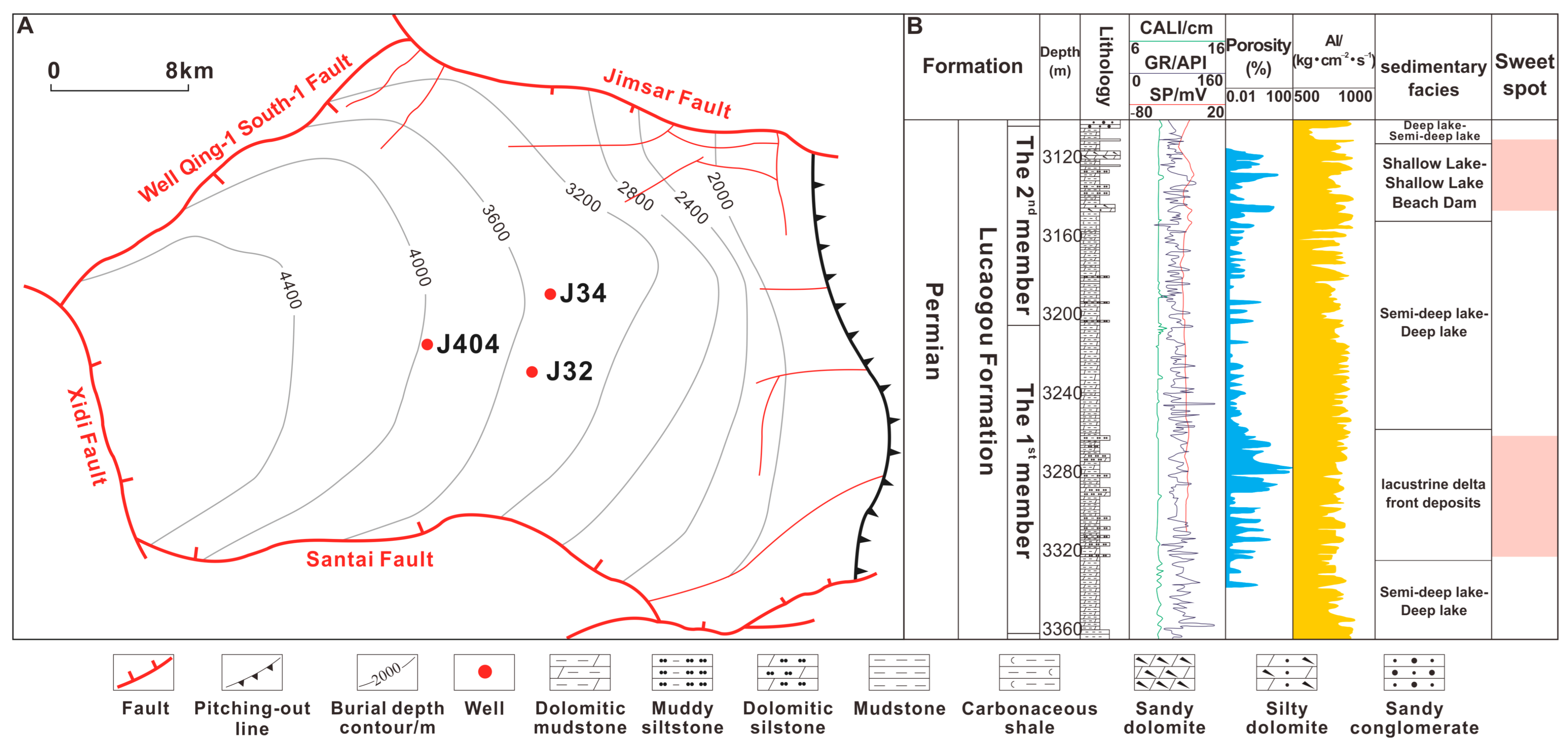
Figure 1. Thickness contour map of the Lucaogou Formation in the Jimusar Sag (A) and the comprehensive stratigraphic column of the Jimusar Sag (B).
Applsci 16 05234 g001
Figure 2. Architecture of the stacking ensemble model.
Applsci 16 05234 g002
Figure 3. Architecture of Random Forest (A), XGBoost (B), LightGBM (C) and CatBoost (D).
Applsci 16 05234 g003
Figure 4. Comparison of AC log data before and after resampling.
Applsci 16 05234 g004
Figure 5. Prediction results of different models: CatBoost ((A1): R2 fit; (A2): residual distribution; (A3): observed vs. predicted values), LightGBM (B1B3), Random Forest (C1C3), XGBoost (D1D3), and stacking ensemble (E1E3).
Applsci 16 05234 g005
Figure 6. Predicted elemental compositions for well JHW87-11.
Applsci 16 05234 g006
Figure 7. Scatter plots showing the effects of different parameters on fracture pressure in well JHW87-11. ((AE): Fracture Pressure vs. conventional logs: AC, GR, CNL, DEN, RI; (FI): Fracture Pressure vs. ECS-derived elemental fractions: Al, Ca, Si, Fe).
Applsci 16 05234 g007
Figure 8. Log-based mechanical interpretation framework and cross-plot correlations among fracture pressure with B I e , E d , and ISIP for well JHW87-11. ((A,B): Well-scale trends of mechanical parameters and pressure: Ble, Ed, ISIP, and measured fracture pressure; (CE): Measured fracture pressure vs. mechanical indicators: ISIP, Ble, Ed; (FH): Predicted fracture pressure vs. mechanical indicators: ISIP, Ble, Ed).
Applsci 16 05234 g008
Figure 9. Cross-plots of elemental compositions versus hydraulic-fracturing response parameters. (Fracture pressure versus elemental composition: Silicon (A) and Calcium (B); Predicted vs. measured fracture pressure and error analysis: predicted vs. measured fracture pressure (C) and relative error distribution (D)).
Applsci 16 05234 g009
Table 1. Optimal hyperparameters of individual models.
Random ForestCatBoost
n_estimators: 600depth: 10
max_depth: 17learning rate: 0.147
min_samples_split: 5l2_leaf_reg: 1.129
min_samples_leaf: 1random_strength: 1.309
XGBoostLightGBM
n_estimators: 500maximum depth: 10
max_depth: 8learning rate: 0.090
learning_rate: 0.041number of leaves: 246
subsample: 0.766subsample ratio: 0.991
colsample_bytree: 0.766feature sampling ratio: 0.746
reg_alpha: 0.004L1 regularization coefficient: 0.004
reg_lambda: 1.629L2 regularization coefficient: 0.049
Table 2. Prediction results for different elements.
ElementnMLR Baseline R2RMSER2MAEMAPE
Al109,8840.813 ± 0.0020.0048 ± 0.00030.849 ± 0.00020.0034 ± 0.00028.65% ± 0.15%
Ca109,8840.805 ± 0.0020.0152 ± 0.00040.851 ± 0.00020.0102 ± 0.0003N.A.
Fe109,8840.832 ± 0.0020.0032 ± 0.00020.876 ± 0.00020.0024 ± 0.00018.01% ± 0.12%
Si109,8840.798 ± 0.0020.0143 ± 0.00040.843 ± 0.00020.0098 ± 0.00034.99% ± 0.10%
Note: n represents the number of valid samples retained for model construction and evaluation after removing the top 5% of outliers using the Mahalanobis distance. Values are reported as mean ± standard deviation across five cross-validation folds. The baseline model corresponds to multiple linear regression using the same input features and validation strategy. MAPE was not calculated for Ca because zero values in the measured Ca data would result in division by zero during MAPE computation.
Disclaimer/Publisher’s Note: The statements, opinions and data contained in all publications are solely those of the individual author(s) and contributor(s) and not of MDPI and/or the editor(s). MDPI and/or the editor(s) disclaim responsibility for any injury to people or property resulting from any ideas, methods, instructions or products referred to in the content.