Article

Deployment and Coverage Optimization Methods for Base Stations Under Multi-Type Terminal Scenarios in 5G-A Industrial Private Network


1
Science and Technology on Electronic Test & Measurement Laboratory, The 41st Institute of China Electronics Technology Group Corporation, Qingdao 266000, China
2
Ceyear Technologies Co., Ltd., Qingdao 266000, China
3
Beijing Zhongxing Digital Nebula Technology Co., Ltd., Beijing 100176, China
*
Author to whom correspondence should be addressed.
Appl. Sci. 2026, 16(11), 5223; https://doi.org/10.3390/app16115223
Submission received: 15 February 2026 / Revised: 9 May 2026 / Accepted: 19 May 2026 / Published: 22 May 2026

Abstract

With the deepening integration of 5G-Advanced (5G-A) technology into smart manufacturing, the large-scale deployment of dynamic terminals—such as mobile robots and automated guided vehicles (AGVs)—within industrial private networks introduces complex, time-varying penetration and path losses. This significantly degrades the accuracy of conventional signal quality and capacity estimation methods, which were primarily designed for static terminal scenarios, thereby posing substantial challenges to coverage and deployment planning of industrial 5G access points, with downstream implications for power capacity dimensioning. To address this problem, this paper proposes a coverage-driven base station deployment optimization method formulated as a combinatorial optimization problem. The study constructs a signal strength assessment and network throughput calculation model tailored for dynamic industrial environments. This model captures the joint impact of terminal mobility and environmental obstacles on signal propagation, thereby enabling more reliable estimation of coverage performance and power consumption. Furthermore, by formulating the base station placement optimization as a combinatorial optimization problem, and by introducing mechanisms for equivalent transformation of the objective function and data preprocessing, the proposed method substantially reduces redundant computations during heuristic iterations. Simulation results verify that, compared with conventional static planning approaches, the proposed scheme enhances both the accuracy and computational efficiency of deployment planning while maintaining coverage quality. This work provides a theoretical foundation and a practical methodology for deploying reliable and energy-efficient industrial 5G-A private networks.

1. Introduction

With the advancement of Industry 4.0 and the proliferation of smart manufacturing, 5G industrial private networks are being widely deployed as critical infrastructure for modern manufacturing. According to GSMA forecasts, the global market for industrial private networks is projected to exceed USD 10 billion by 2026 [1,2,3], underscoring their growing significance in modern industrial ecosystems. 5G technology addresses critical limitations inherent in traditional industrial wireless solutions (e.g., Wi-Fi, Bluetooth, and IEEE 802.15.4-based systems), which suffer from limited coverage, inconsistent network performance, and insufficient terminal connectivity. By leveraging its low-latency, ultra-reliable, and massive-connectivity capabilities, 5G offers superior capacity to support diverse industrial communication requirements. The deployment of 5G wireless services is expected to expand across manufacturing facilities, encompassing both production support systems (e.g., intelligent logistics and surveillance) and core automation processes [4,5,6]. This widespread adoption is expected to drive a substantial increase in wirelessly connected factory equipment. Industrial applications particularly benefit from the enhanced real-time performance of 5G, where low latency and high reliability are paramount. The continuous evolution of 3GPP standards [7,8,9] and the maturation of industrial control technologies are further strengthening 5G/5G-A URLLC capabilities. These improvements are reflected in reduced communication latency and enhanced network dependability, rendering 5G increasingly suitable for time-critical industrial automation applications. Consequently, the penetration rate of wireless connectivity in industrial equipment is anticipated to grow substantially. 5G networks exhibit broad applicability across multiple industrial domains, including manufacturing, mining, energy, ports, automotive, and renewable energy sectors. According to data from the Ministry of Industry and Information Technology (MIIT) of China [10], the Global mobile Suppliers Association (GSA), and industry research reports, 5G implementation in industrial settings has progressively evolved from peripheral support functions (e.g., video surveillance and logistics management) to core control operations (e.g., remote manipulation and collaborative robotics). As illustrated in Figure 1 from the MIIT’s global analysis [11] of 5G industrial applications, the renewable energy operations and maintenance sector currently exhibits the highest adoption rate of 5G communication technologies.
However, the increasing density of base station deployments in industrial environments has led to substantial growth in power consumption. Industry analyses indicate that base station energy consumption accounts for approximately 40% of total operational costs, with signal-quality-induced energy fluctuations emerging as a critical bottleneck for energy efficiency optimization in industrial private networks [12,13,14,15]. Concurrently, the proliferation of artificial intelligence has driven the large-scale deployment of intelligent terminals in industrial settings, including automated guided vehicles and smart handling robots. These mobile devices introduce dynamic variations in channel attenuation, significantly affecting throughput estimation in the communication space. Consequently, conventional throughput models and power planning methods designed for static scenarios are inadequate for industrial private networks characterized by numerous mobile terminals and large-scale production equipment. This presents a pressing challenge for network operators: how to optimally determine base station locations and power capacity during the planning phase so as to control energy consumption and reduce operational costs. The existing literature approaches this problem from multiple perspectives. Regarding signal propagation characteristics, prior studies have primarily focused on general 5G communication theories and models. While conventional models such as COST-231-Hata [16] and Okumura-Hata [17] are widely adopted for macro-scale propagation prediction, their accuracy in industrial environments remains limited. Industrial settings present unique challenges owing to the abundance of metallic equipment, complex structural layouts, and human activity, resulting in intricate path loss and multipath effects that conventional models fail to characterize adequately. Several studies have attempted to modify and improve these traditional models for specific industrial scenarios. For instance, Tanghe et al. [18] proposed a modified one-slope model calibrated for industrial environments with heavy machinery, while Ai et al. [19] extended the COST model to account for metallic reflections in factory halls. Nevertheless, a model applicable to diverse industrial environments has yet to be established.
For base station throughput estimation, traditional methods typically rely on theoretical maxima or empirical values. These approaches often fail to account for practical factors such as signal quality fluctuations and terminal performance variations, leading to notable discrepancies between estimated and measured performance. Some studies have begun to explore throughput calculation methods based on field measurement data. However, the difficulty and cost of data acquisition, coupled with the absence of systematic data processing methodologies, have limited the broader adoption of these approaches. In the field of base station power consumption, existing research primarily focuses on analyzing the energy consumption characteristics of base station equipment and investigating energy-saving technologies such as energy efficiency ratios and sleep mode switching. For instance, Ref. [20] proposed an online algorithm based on the Lyapunov framework [21,22] to jointly optimize video quality and energy consumption for base stations equipped with energy harvesting capabilities. The authors of [23] investigated the use of renewable energy in cellular networks under high-traffic conditions to reduce grid dependency and carbon emissions, thereby enabling base stations with a high proportion of renewable energy to serve more users. Additionally, Ref. [24] studied the optimal sleep strategy for a single base station, formulating the sleep optimization problem—which considers key factors such as handover energy consumption and delay performance—as a partially observable Markov decision process (POMDP) [25,26,27,28], thereby reducing the energy consumption of the communication system. However, there is limited research on accurately calculating the power consumption of base stations based on their throughput demands. Most existing studies fail to fully account for the dynamic relationship between throughput and power consumption, lacking a comprehensive framework that links network performance requirements to energy consumption assessment. This gap makes it difficult to achieve precise planning of base station power capacity. In summary, the existing body of work exhibits the following deficiencies in the power capacity planning of industrial private network base stations. First, the characterization of signal propagation in industrial environments lacks sufficient accuracy. Second, existing throughput calculation methods do not adequately reflect the characteristics of practical industrial scenarios. Third, a systematic quantitative framework linking signal quality, throughput, and power consumption remains absent. These deficiencies result in inaccurate power capacity planning during the deployment of 5G industrial private networks, making it difficult to satisfy the stringent reliability and efficiency requirements of industrial production. Therefore, this study addresses the issue of unstable signal strength in industrial private networks. By precisely modeling the movement trajectories of terminals and the distribution characteristics of obstacles, it proposes a systematic approach—from signal strength modeling to throughput calculation, and subsequently to access point location selection, with post-processed power capacity estimation provided as a downstream step—to provide a more scientifically grounded solution for the coverage-driven deployment of 5G industrial private network base stations. The proposed method provides a systematic framework for coverage-driven deployment that serves as the basis for subsequent power capacity dimensioning, potentially reducing over-provisioning in industrial private networks.
The main contributions of this paper are summarized as follows:
(1)
Within a complex three-dimensional (3D) industrial environment, a signal strength model tailored to the non-homogeneous propagation medium of industrial settings is constructed using real-world measurement data. This model quantifies the impact of obstacle-specific penetration and path losses on signal propagation.
(2)
Building upon the channel loss model, an enhanced throughput calculation model is presented. This model characterizes the throughput behavior in industrial private networks where mobile and fixed terminals coexist.
(3)
A coverage-driven AP deployment optimization problem is formulated as a combinatorial problem with the AP locations as decision variables and the weighted average received signal strength as the objective, subject to a coverage reliability constraint. The optimized deployment can subsequently be used as the input to a downstream post-processing step in which the per-AP power capacity is estimated, as illustrated in Section 3.1.

2. System Configuration and Modeling

This section establishes the analytical foundation for the deployment optimization framework. The signal propagation model (Section 2.1) and the communication throughput model (Section 2.2) together define the mapping from base station, which is normally defined as an access point (AP) in system modeling, locations to coverage quality metrics. The propagation model provides the received signal strength at each terminal for a given AP position, while the throughput model translates signal strength into achievable data rates. These models are intentionally kept computationally lightweight to enable the exhaustive heat map pre-computation described in Section 3, where the signal strength from every candidate AP position to every terminal must be evaluated. The resulting heat maps then serve as lookup tables for the optimization algorithm, eliminating propagation calculations during the iterative search.

2.1. Three-Division Industrial Scenario Description

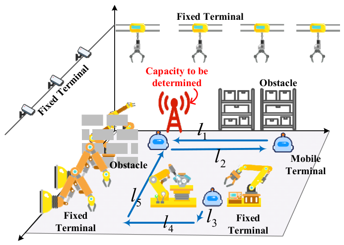
The topological distribution of the industrial scene considered in this paper is derived from the wireless production workshop of the 41st Research Institute of China Electronics Technology Group Corporation. In this scenario, s fixed terminals and m mobile terminals are deployed. There are also some obstacles of different materials, sizes, and positions. Their three-dimensional size and attenuation parameters for wireless signals are known, and the traveling paths and coordinates of the mobile terminals are also known. At this point, the deployment locations of the N a APs on the ceiling plane are the variables to be determined. The corresponding power capacity requirement of each AP is computed in a post-processing step described in Section 3.1, after the optimal AP locations have been obtained.
To describe the three-dimensional layout information of the industrial site and the positions of various terminals, the scene diagram in Figure 2 is transformed into a three-dimensional spatial coordinate system, with the Z-axis representing the height relative to the ground in the vertical direction. To enhance the solution efficiency, in this paper, the domain is discretized, and the three-dimensional interval is divided into block cubes with length, width, and height all of k. The number of cube blocks divided in the x, y, and z directions of the scene is denoted as D x , D y , and D z respectively. The combination of each discretized cube can be approximately represented as an obstacle and a fixed terminal, and the path of the mobile terminal is based on the combination of several consecutive cube blocks it passes through in its action path. In this article, the mobile terminals are taken as examples of patrol robots and material handling robots. The movement path of the patrol robot is a straight line from l 3 to l 5 , while the material handling robot performs material handling tasks between two points, with a path of two opposite and overlapping line segments from l 1 to l 2 . The detailed modeling assumptions underlying the subsequent analysis are formally summarized in Section 2.2.

2.2. System Modeling Assumptions

To establish a tractable yet realistic framework for AP deployment optimization in industrial private 5G networks, the following modeling assumptions are adopted throughout this work. These assumptions collectively define the scope and applicability of the proposed methodology.
(1)
Frequency Band and Bandwidth: The system is assumed to operate in the 5G NR FR1 spectrum at a carrier frequency of 3.5 GHz, with a nominal bandwidth of 100 MHz. This frequency band is widely used in industrial private network deployments because it offers a favorable balance between coverage and capacity.
(2)
AP Antenna Configuration: Each AP is assumed to be equipped with an omnidirectional antenna for coverage planning. Although the effects of directional antennas or beamforming could be incorporated by modifying the antenna gain term in the link budget, they are not explicitly considered in this study.
(3)
Deployment Plane: All APs are ceiling-mounted at a fixed height H c e i l above the factory floor. The optimization is therefore restricted to the two-dimensional ceiling plane coordinates ( x i , y i ) This reflects common industrial deployment practice where APs are installed overhead to maximize line-of-sight probability.
(4)
Terminal Types and Traffic Demand: Fixed Terminals: Represented by stationary sensors, cameras, or control panels at known 3D coordinates. Each fixed terminal is assumed to require a constant throughput demand D f i x e d (e.g., 10 Mbps) for uplink/downlink communication.
Mobile Terminals: Represented by AGVs, patrol robots, or handling robots moving along pre-defined, deterministic trajectories. The trajectory of each mobile terminal is discretized into a sequence of equally spaced waypoints. Each mobile terminal is assumed to require a constant throughput demand D m o b (e.g., 5 Mbps) at every point along its path.
(5)
Obstacle Representation: Obstacles such as machinery, metal racks, and partition walls are modeled as axis-aligned bounding boxes (AABB) with known dimensions, positions, and material-specific penetration losses. The penetration loss values are obtained from on-site measurements or standard material property tables. The ray-tracing intersection test considers only line-of-sight blockage; diffraction and reflection effects are neglected, which is acceptable for coverage planning at sub-6 GHz frequencies in open industrial halls.
(6)
Interference Management: The deployment optimization assumes orthogonal resource allocation among APs (e.g., via different frequency sub-bands or time slots). Consequently, co-channel interference is neglected in the coverage prediction phase. This assumption is reasonable for initial planning stages where the number of APs is small relative to available spectrum resources.
(7)
Mobility Model: Mobile terminals traverse straight-line trajectories between designated waypoints at a constant speed. Temporal dynamics such as Doppler spread are accommodated through a link margin embedded in the coverage threshold rather than through explicit time-varying channel modeling.
(8)
Scheduler: A round-robin scheduler is assumed for resource block allocation among associated terminals.
The propagation model adopted in this work captures two dominant attenuation mechanisms: distance-dependent path loss and obstacle penetration loss. Several secondary propagation effects are not explicitly modeled but are addressed within the framework as follows.
(1)
Thermal noise is incorporated in the SINR calculation in Equation (7), where the noise power is computed as N 0 = k B T 0 B .
(2)
Reflection, diffraction, and scattering contribute primarily to small-scale fading. In the open industrial hall considered here, the dominant propagation path is direct LoS or obstructed LoS, and multipath components are secondary. The aggregate effect is accommodated through a fade margin of 8–10 dB embedded in the coverage threshold P min rather than through explicit multipath ray tracing. This is a standard practice in coverage planning and is consistent with the 3GPP Indoor Factory (InF) channel model framework in TR 38.901, which separates deterministic large-scale path loss from stochastic small-scale fading.
(3)
Body blockage from mobile terminal operators is accounted for within the fade margin included in P min .
This deterministic modeling approach is intentionally chosen to enable exhaustive heat map pre-computation (Section 3), where the signal strength from every candidate AP position to every terminal must be evaluated. A stochastic fading model would require Monte Carlo averaging at each grid point, increasing the pre-computation cost by orders of magnitude without materially improving the deployment decision, since the optimization targets median coverage quality rather than instantaneous channel realizations. Furthermore, the framework is modular: should a site-specific measurement campaign yield a calibrated fading model, it can be incorporated by adjusting the fade margin or replacing the path loss equations.

2.3. Channel Model and Spatial Signal Strength Modeling

Communication signals will experience attenuation when they propagate in the air or pass through obstacles. This paper models the propagation channel of electromagnetic waves in wireless communication to quantitatively describe the path loss and penetration loss of AP signals during their propagation. This paper uses a large-scale model to depict the AP signals received at the receiving end that have undergone long-distance propagation. The logarithmic distance attenuation model can be expressed as:
P L = P L ( d 0 ) + 10 φ lg d d 0
where the P L represents the signal attenuation that occurs at the receiver after the signal is transmitted by the AP and undergoes path loss. d 0 is the Euclidean distance from the AP to the terminal, which is the standard reference distance, usually valued at one meter. P L ( d 0 ) is the actual signal strength received at the reference point from the AP, and φ is the path loss coefficient, whose value is related to the specific propagation environment. When the distance between the AP and the terminal is constant, even if the positions of the AP and the terminal are different, the loss of the signal transmitted by the AP reaching the terminal is only related to the straight-line distance between the two.
In addition to the path loss modeled above, there is also penetration loss caused by obstacles in industrial scenarios. After comprehensively considering the path loss and penetration loss, the channel attenuation of the signal transmitted from the i-th AP to the j-th terminal in a non-uniform medium can be expressed as:
P L ( i , j , θ ) = P L ( d 0 ) + 10 φ lg d i j + k N b α i , j , k β k
where the P L ( i , j , θ ) represents the signal attenuation at the j-th terminal after considering the path loss and penetration loss of the signal emitted by the i-th AP. θ is the set of obstacles in the scene, with β k representing the penetration loss of the k-th obstacle in this set. α i , j , k indicates whether the signal emitted by the i-th AP has penetrated the k-th obstacle on its path to the j-th terminal, that is:
a i , j , k = 0 ,   The   signal   did   not   penetrat   the   obstacle 1 ,   The   signal   penetrated   the   obstacle
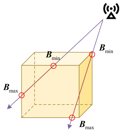
In order to determine the α i , j , k value, it is necessary to observe in the three-dimensional scene whether the rays from the AP towards the terminal pass through the obstacles. In this paper, the Axially Aligned Bounding Box algorithm [29], which is widely used in optical line tracing, is used to determine the intersection relationship of the rays between the AP and the terminal. In 5G signal propagation modeling, obstacles such as buildings can be simplified as bounding boxes. Through this algorithm, it can be quickly determined whether the rays (signal propagation paths) emitted by the AP intersect with the obstacles. Let the R ( t ) equation of the ray emitted by the AP be:
R ( t ) = O + t D   ( t > 0 )
where O = ( O x , O y , O z ) is the location of the AP; D = ( D x , D y , D z ) is the vector of the signal propagation direction. In this paper, an axially aligned enclosing cube is used to characterize the signal propagation path. The axially aligned enclosing bodies of the obstacles are respectively composed of the minimum vertices B min = ( B x min , B y min , B z min ) and maximum vertices B max = ( B x max , B y max , B z max ) set. Figure 3 is a schematic diagram of the Axially Aligned Bounding Box. Calculate the time for the rays to enter and exit the bounding box for each coordinate axis:
t x min = B x min O x D x ,   t x max = B x max O x D x t y min = B y min O y D y ,   t y max = B y max O y D y t z min = B z min O z D z ,   t z max = B z max O z D z
If B min B max and B min 0 , then the ray intersects with the bounding box. The signal strength received by the mobile terminal in an industrial scene can be represented through the ray tracing algorithm as:
P i , j = P A P L ( i , j , B )
where the P A is the power of the signal transmitted by the AP, and P L ( i , j , B ) is the attenuation of the signal transmitted by the i-th AP at the j-th terminal.
The log-distance path loss model with additive penetration loss is adopted as the primary propagation model in this work. While more sophisticated models incorporating Rayleigh or Rician fading could improve prediction accuracy, the deterministic path loss model is considered adequate for the following reasons. First, the coverage planning objective targets the median received signal strength rather than instantaneous fading realizations; small-scale fading effects are accommodated through a fade margin of 8–10 dB included in the minimum receiving level threshold P min . Second, the industrial hall considered in this study features predominantly line-of-sight (LoS) or obstructed-LoS propagation paths, where the deterministic component dominates over stochastic fading. Third, the penetration loss model explicitly accounts for the dominant source of signal degradation in industrial environments, namely blockage by large metallic obstacles, which is not captured by statistical fading models. This modeling choice is consistent with the 3GPP InF (Indoor Factory) channel model framework specified in TR 38.901 [30], which separates deterministic large-scale path loss from stochastic small-scale fading components. Furthermore, the proposed framework is modular: should a more detailed propagation model become available for a specific factory environment, it can replace the current path loss equations without altering the heat-map-based optimization algorithm.

2.4. Communication Throughput Model

In the context of industrial private networks, the throughput model of 5G APs needs to comprehensively consider channel characteristics, resource allocation, interference management, and reliability requirements. This paper models the communication throughput based on the classical Shannon theory, providing necessary data references for the subsequent calculation of AP power capacity. The classic Shannon theory can be expressed as:
C = η B log 2 ( 1 + S N + I )
where the C is channel capacity, B is available bandwidth, S denotes the received signal power, N is the noise power, I denotes the undesired signal, and 0 < η < 1 means the system efficiency factor.
In the SINR expression, the received signal power P s at terminal j from its serving AP i is computed as P s = P t L i j , where L i j is the total channel attenuation given by Equation (2). The noise power is calculated as N 0 = k B T 0 B , where k B is the Boltzmann constant, T 0 = 290   K is the reference temperature, and B is the allocated bandwidth. Under the orthogonal resource allocation assumption stated in Section 2.2, co-channel interference I is set to zero for the coverage planning phase. The spatial multiplexing gain min ( N , K ) in Equation (8) reflects the degrees of freedom available in a multi-antenna system. For the omnidirectional single-antenna configuration assumed in this work, N = 1 , and the multiplexing term reduces to unity.
Considering the existence of multiple terminals in industrial scenarios, this paper extends the above model to:
C m = min ( N , K ) η B log 2 1 + S N + I
where the N represents the number of AP antennas and K represents the number of terminals; min ( N , K ) indicates the spatial multiplexing gain.
In industrial scenarios, resource blocks (RBs) are allocated to multiple users or slices. Suppose the total number of resource blocks is N R B , and each user is allocated n R B , then the throughput can be expressed as:
C s u m = i = 1 K ( η n R B , i Δ f log 2 1 + S i N + I i )
where Δ f represents the bandwidth of a single RB. In this paper, the value is taken according to the 5G R17 standard, and K is the number of users scheduled simultaneously. Industrial scenarios require high reliability (such as 99.99%), and redundancy ξ (such as HARQ retransmission) and low-bitrate coding needs to be introduced. The actual effective throughput is:
C e = C t ( 1 ξ ) η s
where ξ denotes the redundancy overhead factor and η s denotes the scheduling efficiency factor for round-robin allocation. For URLLC services with a reliability target of 99.99%, ξ is set to 0.25 based on 5G NR link-level simulation results, which represents a 25% throughput reduction. The total number of available resource blocks N R B is determined by the system bandwidth according to 3GPP TS 38.214 [13]; for a 100 MHz bandwidth at 3.5 GHz, N R B = 273 with a subcarrier spacing of 30 kHz, yielding a per-RB bandwidth of B R B = 360   kHz .

3. Signal Coverage Optimization and AP Deployment Based on Heat Map

In this section, we formulate the AP deployment problem for industrial private 5G networks and present a computationally efficient heuristic solution. Notably, while end-to-end network engineering often includes power capacity dimensioning, the scope of the present work is strictly limited to AP placement optimization. For a fixed number of APs, we seek to determine optimal ceiling-mounted locations that maximize coverage performance for both fixed and mobile terminals. In Section 3.1, we briefly outline the relationships among coverage, throughput, and power consumption to establish the necessary context and to show how optimized deployment results can serve as a solid basis for subsequent power capacity planning. The optimization algorithm developed in Section 3.2 and Section 3.3, however, focuses exclusively on location optimization, with power capacity treated as a derived metric rather than a jointly optimized decision variable.

3.1. Coverage–Power Consumption Relationship of APs

Based on the previously derived channel model, the relationship between achievable throughput and the required transmit power can be expressed by inverting the Shannon capacity formula:
T = B log 2 1 + P t x G l i n k η B W σ 2 + I
where T (bps) denotes the throughput, P t x (W) is the output power, B (Hz) is bandwidth, G l i n k is the link gain that incorporates path loss, penetration loss, and antenna gains, η B W denotes the efficiency factor for bandwidth, σ 2 is the noise power, and I is the interference signal power. The link gain g corresponds to the inverse of the total channel attenuation, i.e., G l i n k = L i j .
Solving the above equation can yield the required AP transmission power:
P t x = ( 2 T / B 1 ) ( σ 2 + I ) G l i n k η B W
This paper establishes a separation model of static power amplifiers P s and dynamic power consumption based on the physical architecture of AP equipment and reveals the nonlinear dependency relationship between this model and business load.
P t o t a l = P s + P t x ( T ) η P A + α T
P t x ( T ) represents the cascading mapping among throughput T , transmission power P t x , and total power consumption P t o t a l . By quantifying the power amplifier efficiency η P A and baseband processing coefficient α , in multi-AP power planning, the above-mentioned AP model provides key constraints for system-level optimization problems. where P s denotes the static hardware power consumption (typically 20–40 W for small-cell APs), η is the power amplifier efficiency (typically 0.2–0.35 for Class-B amplifiers).
The real-time power consumption of each AP needs to be met as:
P s + P t x , i ( t i ) η P A , i + α i t i P i max ,   i B
Among them, t i is the throughput load allocated by the AP i , and this constraint directly depends on P t x , i ( t i ) derived from the single AP model to ensure that the optimization results comply with the physical limitations of the equipment. The total power consumption P t o t a l response function generated by the above AP model can provide a computable objective function and gradient information for the convex optimization solution algorithm used in the rest of this paper.
The formulations above establish a deterministic mapping from a given AP location and its associated terminals to the required transmit power and total power consumption. In a full-scale network planning workflow, these equations would be employed after the AP locations have been fixed. This paper does not attempt to jointly optimize locations and power capacities. Instead, this work focuses on the preceding and computationally challenging step. It aims to find the AP locations that provide robust coverage in a complex three-dimensional industrial environment. The power mapping is provided here solely to demonstrate how the coverage results obtained by the proposed algorithm can be translated into practical power provisioning estimates. After the optimal AP locations are determined, the required power capacity for each AP can be estimated as a post-processing step. For completeness, the estimation procedure is outlined as follow.
Let B = 1 , 2 , 3 , , N be a set of N Aps; let D t o t a l be the total throughput demand of all terminals in the industrial site. After user association (e.g., each terminal connects to the AP providing the strongest received signal), the throughput load assigned to AP i denoted by ρ i .The load distribution naturally satisfies:
i = 1 N ρ i = D t o t a l , 0 ρ i C i max
where C i max is the maximum throughput that AP i can support given its location-dependent channel conditions. Using the power-load mapping derived in Equations (13) and (14), the required power capacity P i c a p for AP i is then calculated as:
P i c a p = f p o w ( ρ i , G i )
where G i denotes the vector of channel gains from AP i to its associated terminals.
The above power estimation is included solely to clarify how signal coverage optimization results can be applied within a complete AP planning workflow. In the next subsection, this work focuses on solving the AP placement problem that maximizes coverage for user equipment in industrial scenarios with dynamic terminals. The power estimation results derived from this procedure are reported in Section 4.

3.2. Problem Modeling for Coverage-Optimal AP Location

The industrial scene involved in this study has the characteristic of non-uniform signal transmission, with irregular obstacles distributed in its three-dimensional space, making it difficult to conduct precise modeling through analytical expressions. Furthermore, the movement trajectories of mobile terminals also lack effective mathematical representation methods, which poses significant challenges for traditional integer programming methods (such as the cut plane method, branch and bound method, etc.) in solving this problem. Given that the problem of AP optimal deployment has been proven to be an NP-hard problem [31], that is, there is no exact solution with polynomial time complexity, the adoption of heuristic algorithms becomes a reasonable choice to balance the solution efficiency and the quality of the solution. Heuristic algorithms, as a type of intelligent optimization method, obtain approximate optimal solutions within a limited time through a directional search mechanism, demonstrating good adaptability in solving such complex optimization problems. When using heuristic algorithms to solve the AP optimization deployment problem described in this chapter, there are two main solution strategies:
  • Direct solution method: During each iteration, based on the current AP location deployment plan, the signal strength at each terminal location within the scene is recalculated, and the original objective function is directly optimized. Ultimately, the AP deployment plan that optimizes the objective function is selected as the solution. This method has a relatively high calculation accuracy, but it requires the repeated calculation of the scene, terminal position and signal propagation characteristics in each iteration, resulting in a relatively high computational overhead.
  • Indirect solution method: Through problem transformation, a new objective function with lower computational complexity is constructed. During the iterative process, this alternative function is optimized instead of the original objective function, and its optimal solution is taken as the final deployment scheme. This method improves the solution efficiency by reducing repetitive calculations, but it is necessary to ensure that the alternative function can effectively reflect the optimization objective of the original problem.
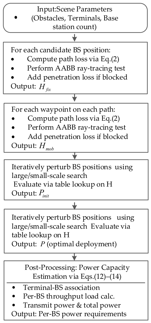
In the AP optimization deployment problem of this paper, the scene layout, the position of fixed terminals and the trajectory of mobile terminals are all prior information and remain unchanged during the solution process. If the direct solution method is adopted, the static information needs to be recalculated in each iteration round, which will introduce a large amount of redundant computations and significantly reduce the algorithm efficiency. Therefore, the algorithm in this section adopts an indirect solution strategy. The calculation process is shown in Figure 4. Through reasonable transformation of the objective function and data preprocessing, the repeated calculation of invariants in the heuristic search process is avoided, thereby significantly improving the calculation speed while ensuring the quality of the solution.
The deployment problem addressed in this work is stated formally as follows. We consider a 3D industrial layout with known obstacle positions and materials, a set of fixed terminals T f with known coordinates, and a set of mobile terminals T m each following a pre-defined spatial trajectory. The trajectory of each mobile terminal is discretized into a sequence of waypoints, denoted by W m = w m 1 , w m 2 , , w m q . The total number of APs N is given.
Variables:
The optimization variables are the 2D ceiling plane coordinates of the N APs:
P = p 1 , p 2 , , p N ,   p i = ( x i , y i )
The installation height is fixed.
Objective Function:
We aim to maximize a weighted sum of the average received signal strength at fixed terminals and along mobile terminal paths:
F ( P ) = α 1 T f j T f S j ( P ) + 1 m T m Q m m T m q = 1 q S m q ( P )
where S j ( P ) is the received signal strength (in dBm) at fixed terminal j from its best-serving AP, and S m q ( P ) is the received signal strength at the q-th waypoint of mobile terminal m. The weights α and β control the relative importance of fixed and mobile coverage.
Constraints:
  • Coverage threshold: At least a fraction η   ( e . g . ,   η = 0.95 ) of all discrete terminal locations—comprising all fixed terminal positions and all waypoints along mobile paths—must have a received signal strength greater than or equal to the receiver sensitivity P s e n   ( e . g . ,   75   dBm ) . Formally,
j m , q S > P sen T f + m Q m η
where the received strength S is taken from the best-serving AP for each location.
2.
Location feasibility: All AP locations must lie within the admissible ceiling area Ω ⊂ R2, that is, p i Ω ,   i = 1 , , N . The problem defined by Equations (18) and (19) is NP-hard, as it generalizes the well-known facility location problem with non-convex coverage regions induced by obstacles. Exact methods are therefore intractable for practical industrial scales, which motivates the heuristic approach developed in the following subsections.

3.3. Heuristic Algorithm for AP Location Optimization

With the terminal-specific signal strength heat maps, the deployment optimization problem defined in Section 3.2 can be solved efficiently. The key advantage of using heat maps is that coverage evaluation for any candidate AP location set P becomes a table lookup operation, eliminating the need for repeated ray-tracing computations during the search process. In this subsection, we first describe how an initial feasible solution is constructed from the heat maps, and then present the iterative search procedure that refines the deployment to maximize the coverage objective.
Overall workflow of the proposed coverage-driven deployment optimization framework. Algorithms 1 and 2 construct the signal strength heat maps that serve as lookup tables for the subsequent optimization. Algorithm 3 generates a high-quality initial solution via greedy sequential placement, which is then refined by the heuristic search in Algorithm 4. The post-processing step translates the optimized AP locations into per-AP power capacity requirements.
Algorithm 1 Heat map of AP signal strength at fixed terminals
Input: Fixed terminal quantity N S , the number of spatial blocks D x , D y , and D z in the x, y, and z directions of the three-dimensional space; the transmission power P A of the AP; The minimum acceptance level of the terminal is P 0 ; fixed terminal location set S ; obstacle set B .
Output: Heat map matrix H n , i j s of AP signal strength for fixed terminals. H n , i j s ,   n 1 , , N s ,   i 1 , , D x
Pseudocode:
1: Initialize H_fix as a |T_f| × N_x × N_y array filled with −∞
2: for each fixed terminal j ∈ T_f do
3:   for x = 1 to N_x do
4:     for y = 1 to N_y do
5:     p_AP ← (x·d, y·d, H_ceil) // candidate AP position
6:     Compute path loss PL(p_AP, p_j) using Equation (1)
7:     Compute penetration loss L_pen via ray-tracing (Equations (2)–(5))
8:     P_r ← P_t ← PL ← L_pen
9:     H_fix[j][x][y] ← P_r
10:    end for
11:  end for
12: end for
13: return H_fix
Algorithm 1 describes the method for generating AP signal strength heat maps for fixed terminals. For each fixed terminal, the algorithm traverses all the cubic blocks within the industrial field area, calculates the two-dimensional AP signal strength heat map at the ceiling height, and outputs it as an AP signal strength heat map matrix of size, representing the AP signal strength.
Algorithm 2 Heat map of AP signal strength for mobile terminals
Input: The number of mobile terminals N m , the number of spatial blocks D x and D y in the x, y, and z directions in three-dimensional space; the position matrix T of cube blocks on the mobile terminal path and the number Q of cube blocks on each mobile terminal path; obstacle set B, the transmission power P A of the AP, and the minimum receiving level P 0 of the terminal;
Output: Heat map matrix H m of AP signal strength for mobile terminals H n , k , i j m ,   n 1 , , N m ,   k Q 1 , , Q N m
Pseudocode:
1: Let total_waypoints ← sum_{m} Q_m
2: Initialize H_mob as a total_waypoints × N_x × N_y array filled with −∞
3: idx ← 0
4: for each mobile terminal m do
5:   for each waypoint w ∈ W_m do
6:     for x = 1 to N_x do
7:      for y = 1 to N_y do
8:       p_BS ← (x·d, y·d, H_ceil)
9:       Compute PL and L_pen between p_AP and w
10:      P_r ← P_t← PL ← L_pen
11:      H_mob[idx][x][y] ← P_r
12:     end for
13:    end for
14:    idx ← idx + 1
15:  end for
16: end for
17: return H_mob
Algorithm 2 describes the method for generating AP signal strength heat maps for mobile terminals. For each cube block in the path of each mobile terminal input, the algorithm traverses all cube blocks within the industrial site area and finally outputs the heat map matrix of all cube blocks on the mobile terminal’s movement path. Next, using the AP signal strength heat maps of the mobile terminal and the fixed terminal obtained earlier, in the AP signal strength heat maps of each cube block in the path between each fixed terminal and each mobile terminal, the position of the cube block with the highest heat value is respectively found, and in a two-dimensional matrix E representing the industrial field plane, Record the contribution of each position that achieves the highest heat value to the initial solution.
For fixed terminals, the contribution of N s is calculated at the corresponding position in E for the cube block that has obtained the highest heat in the AP signal strength heat map of each fixed terminal. For mobile terminals, the contribution of N s is calculated at the AP signal strength heat map of each cube block in the path of the N th mobile terminal, and then, the contribution levels achieved at each position of E are sorted. The positions at the scene ceiling corresponding to the top N a positions with the highest contributions can be used as the initial solution for AP deployment.
Algorithm 3 Initial solution generation algorithm for ap deployment locations based on ap signal strength heat maps
Input: The number of spatial blocks D x and D y in the x and y directions in three-dimensional space, and the number of APs N a ; fixed number of terminals N s ; the number of mobile terminals in N m and the heat map matrix H s of the AP signal strength of fixed terminals; heat map matrix H m of path signal strength for mobile terminals.
Output: The initial solution generates the matrix scaling coefficient N d ;
1: Initialize accumulator matrix E of size N_x × N_y with zeros
2: // Process fixed terminals
3: for each fixed terminal j do
4:   Find (x*, y*) that maximizes H_fix[j][x][y]
5:   E[x*][y*] ← E[x*][y*] + α
6: end for
7: // Process mobile waypoints
8: for each waypoint index w (from 1 to total_waypoints) do
9:   Find (x*, y*) that maximizes H_mob[w][x][y]
10:   // Distribute weight β evenly among waypoints of the same mobile terminal
11:  weight ← β/(number of waypoints for this terminal)
12:  E[x*][y*] ← E[x*][y*] + weight
13: end for
14: // Select top N distinct grid positions with highest E scores
15: P_init ← indices of top N values in E
16: return P_init
Algorithm 3 describes the initial solution generation algorithm for AP deployment locations based on the AP signal strength heat map. The algorithm respectively targets all AP signal strength heat maps with cubic blocks in each fixed terminal and each mobile terminal path to find the point with the highest heat value, and accumulates the corresponding contribution in E i j .
Algorithm 4 Deployment location solution algorithm based on AP signal strength heat map
Input: Initial solution P 0 ; fixed terminal number N s , mobile terminal number Nm; AP number N a ; the number of spatial blocks D x , D y , and D z in the x, y, and z directions in three-dimensional space; heat map matrix H s of AP signal strength for fixed terminals; heat map matrix H m of path AP signal strength for mobile terminals;
Output: AP deployment location P;
1:  Initialize population: S_k ← P_init for k = 1, N_p
2:  P* ← P_init; f* ← Evaluate(P_init, H_fix, H_mob)
3:  for iter = 1 to MC do
4:    for k = 1 to N_p do
5:     S_new ← S_k
6:     Randomly select one AP index r ∈ {1, …, N_a}
7:     Generate u ~ Uniform(0,1)
8:       Δx ~ Uniform(-N_x/2, N_x/2)
9:      Δy ~ Uniform(-N_y/2, N_y/2)
10:    else      //Small-scale search
11:      Δx ~ Uniform(-N_x/(2*C_s), N_x/(2*C_s))
12:      Δy ~ Uniform(-N_y/(2*C_s), N_y/(2*C_s))
13:    end if
14:    S_new(r).x ← S_k(r).x + round(Δx)
15:    S_new(r).y ← S_k(r).y + round(Δy)
16:     // Boundary check
17:    while S_new(r) is outside scene boundary do
18:      Regenerate Δx, Δy as above
19:       S_new(r).x ← S_k(r).x + round(Δx)
20:       S_new(r).y ← S_k(r).y + round(Δy)
21:    end while
22:    f_new ← Evaluate(S_new, H_fix, H_mob) // Table lookup
23:    if f_new > f* and AllTerminalsCovered(S_new, H_fix, H_mob, P_min) then
24:       P* ← S_new; f* ← f_new
25:    end if
26:   end for
27:  // Move population toward best solution
28:   for k = 1 to N_p do
29:    S_k ← P*
30:   end for
31: end for
32: return P*
Function Evaluate(P, H_fix, H_mob):
  f ← 0
  for each fixed terminal j do
   f ← f + α * max_{i∈P} H_fix[j][P_i.x][P_i.y]
  end for
  for each mobile waypoint (m,q) do
   f ← f + (β/Q_m) * max_{i∈P} H_mob[idx(m,q)][P_i.x][P_i.y]
  end for
  return f
8:     if u < p th
In the process of heuristic solution 4, to find a better solution locally while searching for possible better solutions in the entire solution space, in the algorithm of this step, each solution in the solution set will undergo a large-scale search with a probability of p, or a small-scale search with a probability of p, thereby conducting searches on both the local and the entire solution space. In addition, to prevent candidate solutions from moving out of the scene range, when the position of an individual randomly moves out of the scene range, a new position is randomly generated for it repeatedly until the new position is valid. When a small-scale search is conducted, the bounds are,
0 δ x D x 10 ,   0 δ y D y 10
When a large-scale search is conducted, the bounds are,
D x 2 Δ x D x ,   D y 2 Δ y D y
Algorithm 4 describes an AP deployment location solution algorithm based on the AP signal strength heat map. The process of the algorithm includes: 1. Initialize the resolution set and use the initial solution to replicate it N p times for search during the solution process. 2. Conduct iterative solutions. For each individual solution in the solution set of step 1, a large-scale search will be conducted with a probability of p ; otherwise, a small-scale search will be carried out. The global optimal solution and the local optimal solution will be searched respectively. 3. Use the calculated AP signal strength heat map to accelerate the calculation of the objective function values and validity of each solution in the solution set. When the objective function value of a certain individual is better than the historical optimal solution and meets the constraint conditions, the historical optimal solution is updated to that individual. 4. Move all the solutions in the solution set to the positions of the historically optimal solutions. 5. Continue to repeat step 2 until the set number of iterations is reached. Then, stop the iteration and output the historical optimal solution at this point as the result of the heuristic solution.
The heat map is constructed under the assumption that all APs are mounted at a fixed ceiling height, reducing the deployment optimization from a 3D problem to a 2D search over the ceiling plane. This assumption is justified by practical installation constraints in industrial environments, where APs are typically mounted on the ceiling or overhead cable trays to avoid interference with ground-level operations and to maximize LoS coverage alternative mounting heights (e.g., on pillars or walls at intermediate heights) could potentially improve coverage in specific scenarios with tall obstacles, the ceiling-mounted configuration provides the most unobstructed propagation paths in open industrial halls and is the standard practice recommended by equipment vendors. The proposed framework can be extended to incorporate height as an additional optimization variable by constructing 3D heat maps, at the cost of increased computational complexity proportional to the number of candidate height levels.

4. Experimental Results and Discussion

To verify the optimization effect and operational performance of the algorithm proposed in this chapter, this section implements the algorithm described in Section 3.3 using C++ programming and uses MATLAB 2021a for data processing and chart drawing. Simulation experiments are conducted to verify the coverage effect on each terminal after AP deployment and the operational efficiency of the algorithm. The experiments in this section and the subsequent chapters were all conducted in a 50 m × 50 m × 10 m scene.
The obstacles in the scene had heights ranging from 2 m to 5 m and penetration losses ranging from −5 to −20 dB. The parameters used in the experiment of this subsection are shown in Table 1 as follows:
To begin with, the algorithm’s performance is evaluated under the following parameters: 10 fixed terminals (Ns), 10 mobile terminals (Nm) (including one handling robot and one patrol robot), along with 4 APs (Na). Three deployment strategies are compared: (1) Uniform deployment: APs are placed at evenly spaced grid positions on the ceiling plane. For N APs in an L × W area, the positions are determined by a N × N grid partition. (2) Genetic algorithm (GA): A standard GA with population size 60, crossover rate 0.8, mutation rate 0.1, and 100 generations is used as a metaheuristic baseline [32]. The GA directly evaluates the original objective function (including full ray-tracing computation) in each generation. (3) Proposed heat-map-based algorithm: As described in Algorithms 1–4.
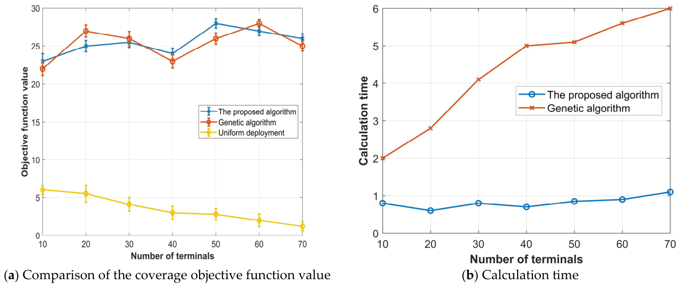
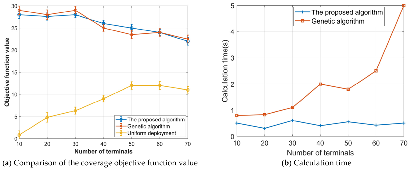
For comparison, the proposed algorithm is benchmarked against a uniform deployment strategy derived from exhaustive enumeration. Each configuration was executed 10 times with different random seeds. The reported values represent the sample mean, and error bars indicate ±1 standard deviation. Across all configurations, the coefficient of variation (CV = σ/μ) of the proposed algorithm remains below 3%, confirming its robustness to random initialization. The results are illustrated in Figure 5 and Figure 6, the vertical axis corresponds to the objective function F ( P ) defined in Section 3.2. Each data point represents the mean of 10 independent trials. Error bars indicate one standard deviation.
It can be seen from the experimental results that in both of the above experimental scenarios, the objective function values corresponding to the solutions obtained by the algorithm proposed in this chapter are much higher than those of the uniformly deployed objective function values in the corresponding experimental scenarios. Moreover, under the premise that the time consumption is much lower than that of the genetic algorithm, the results obtained are almost the same as those of the genetic algorithm. This is because traditional genetic algorithms need to calculate the objective function in each iteration, while the objective function in the problems of this chapter involves the calculation of non-uniform channels in complex three-dimensional industrial scenes. The repeated calculation of the objective function greatly prolongs the calculation time of the genetic algorithm The solution algorithm of the AP signal strength heat map based on the terminal proposed in this chapter avoids the repetitive calculation of the objective function. The proposed method requires less computation time than the GA baseline, which reflects the reduced overhead of the heat-map-based search. Since the optimization is performed offline during the planning stage, this runtime advantage should be interpreted as a supplementary indication of computational efficiency rather than as the primary criterion for assessing the method. Meanwhile, through the AP signal strength heat map, the feasible domain of the AP deployment location can also be known. By using this information, the constraint conditions can be quickly judged, avoiding ineffective random optimization and improving the solution speed. It can also be seen from the figure that the number of mobile terminals has a greater impact on the objective function value than the number of fixed terminals. This is because each cubic block on the path of a mobile terminal is equivalent to multiple fixed terminals, which increases the difficulty of coverage. Therefore, a larger number of mobile terminals will lead to a more significant decrease in the objective function value. Meanwhile, an increase in the number of AP can reduce the difficulty of scene coverage, so the value of the objective function will rise as the number of AP increases. It can also be noted that when the number of mobile terminals increases, the objective function of uniform deployment also rises. This is because the number of each cube block on the mobile terminal path is relatively large. When the position of the AP remains unchanged, increasing the number of mobile terminals can increase the number of cube blocks covered by the AP on the mobile terminal path when the number of mobile terminals is small. This causes the objective function to rise.
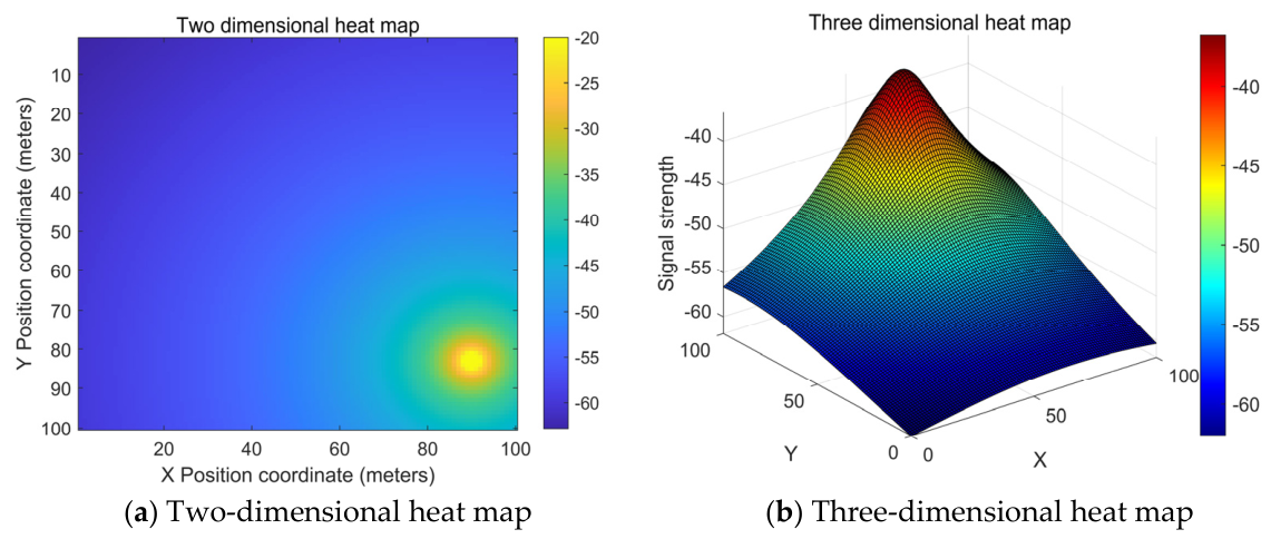
The following figure shows the signal strength heat map results of the optimal deployment location of the AP obtained by solving the algorithm proposed in this paper.
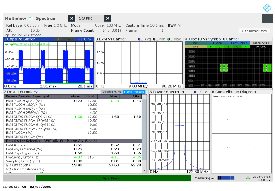
Figure 7 visualizes the received signal strength distribution across the factory floor for the optimized four-AP deployment. The heat map confirms that the proposed algorithm successfully eliminates coverage holes in the vicinity of large metallic obstacles, with all terminal locations receiving signal strength above the −85 dBm threshold. Figure 8 presents the on-site measurement results obtained using R&S vector signal analyzer. The measured EVM values at the designated test points are consistent with the coverage predictions, and a mean absolute error of 1.4 dB is observed between the predicted and measured received signal strength.
Next, verify the improvement of the coverage effect of the algorithm proposed in this chapter on mobile terminals. First, define the cube blocks with signal strength lower than −68 dB in the running path of the mobile terminal as weak cover blocks.
The measurement campaign was conducted using an RS FSW signal analyzer operating at 3.5 GHz with a measurement bandwidth of 100 MHz [33]. A total of four measurement points were selected across the industrial hall, comprising two LoS positions and two NLoS positions. At each point, the received signal strength and EVM were recorded over a 30 s averaging window. Table 2 summarizes the measurement results and their comparison with the model predictions.
Finally, signal quality testing results obtained using a spectrum analyzer (Rohde & Schwarz) positioned at the solution location showed an EVM of less than 1%, validating the effectiveness of the algorithm proposed in this paper. Then, under the conditions of Ns = 80, Nm = 8 and Na taking the smaller value of 6, compare the algorithm, genetic algorithm and uniform deployment method [34] proposed in this chapter. The results are shown in Table 3. Genetic algorithm (GA): A standard GA with population size 60, crossover rate 0.8, mutation rate 0.1, and 100 generations is used as a metaheuristic baseline [35].
It can be seen from the table that when the algorithm proposed in this chapter is used, the proportion of weak coverage blocks in the mobile terminal path is lower than that when the uniform deployment and genetic algorithms are used. This can reflect the effect of the algorithm in this chapter on optimizing the coverage quality of the mobile terminal path. In terms of the uniformity of signal distribution on the mobile terminal path, the AP deployment scheme obtained by the algorithm proposed in this chapter has a lower sum of standard deviations of the cube block signal strength on the mobile terminal path compared with the deployment schemes obtained by the uniform deployment and the genetic algorithm.
According to Equations (13)–(16), after obtaining the optimal AP locations, the power consumption of the APs can be calculated using the following steps:
For each AP i   ( i = 1 , , N ) :
Step 1: Determine the set of associated terminals (each terminal connects to the AP with the strongest signal).
Step 2: Compute the channel gain G i j .
Step 3: Calculate the throughput load of the AP as T i .
Step 4: Obtain the required transmit power according to Equation (12).
Step 5: Calculate the total power consumption using Equation (13).
Power capacity estimation results are listed following in Table 4 and Table 5, where F1~F10 denote the 10 fixed terminals, and M1~M10 denote the mobile terminals.
It should be noted that direct quantitative comparison with existing deployment optimization methods [36,37,38] is challenging due to differences in scenario configurations, terminal types, and optimization objectives. Nevertheless, a qualitative comparison is provided in Table 5 to position the proposed method within the current literature. Where the tick mark “” indicates possession of the feature listed in the first column, while the cross mark “” means the feature is not included.

5. Conclusions

This study investigated the deployment optimization problem for base stations in 5G-Advanced industrial private networks with mixed, fixed and mobile terminals. To address the coverage degradation caused by dynamic terminal mobility and obstacle-induced signal attenuation, we developed a deterministic signal propagation model that incorporates both path loss and penetration loss in an industrial indoor environment. Based on this model, a heat-map-based optimization framework was proposed to efficiently evaluate candidate deployment solutions and identify base station locations that improve overall coverage quality. The proposed method combines pre-computed signal-strength heat maps, a greedy initialization strategy, and a heuristic search algorithm to reduce the computational burden associated with repeated propagation calculations during deployment optimization. This design enables efficient exploration of the placement space while maintaining compatibility with the industrial scenario considered in this work. In addition, a post-processing power estimation procedure was presented to translate the optimized deployment into an indicative per-base-station power requirement, thereby providing a practical reference for subsequent capacity dimensioning. In future work, we will extend the framework in several directions. First, more sophisticated propagation models, such as those incorporating stochastic fading and richer scattering effects, can be integrated to improve modeling fidelity. Second, the deployment problem can be expanded to three-dimensional optimization by allowing AP height to vary. Third, the power estimation module can be further strengthened by jointly considering traffic dynamics, load balancing, and energy-saving mechanisms, so as to move toward a more comprehensive capacity planning framework for industrial private networks.

Author Contributions

Methodology, L.Z.; software, L.Z.; validation, J.Z. (Jingzi Zhan) and J.C.; formal analysis, L.Z.; investigation, J.Z. (Junfeng Zhu); resources, L.Z.; data curation, L.Z.; writing—original draft preparation, L.Z.; writing—review and editing, H.W.; visualization, J.C.; supervision, H.W.; project administration, J.Z. (Jingzi Zhan); funding acquisition, J.Z. (Junfeng Zhu). All authors have read and agreed to the published version of the manuscript.

Funding

This work is supported by the National Natural Science Foundation of China under Grant No. 62127804, and the Stable Support Foundation of CETC Group (41ZQ1499).

Institutional Review Board Statement

Not applicable.

Informed Consent Statement

Not applicable.

Data Availability Statement

The original contributions presented in this study are included in the article. Further inquiries can be directed to the corresponding author.

Conflicts of Interest

The authors declare that this study received funding from The 41st Institute of China Electronics Technology Group Corporation, Ceyear Technologies Co., Ltd. and Beijing Zhongxing Digital Nebula Technology Co., Ltd. The funder was not involved in the study design, collection, analysis, interpretation of data, the writing of this article, or the decision to submit it for publication.

References

  1. Mahmood, A.; Beltramelli, L.; Abedin, S.F.; Zeb, S.; Mowla, N.I.; Hassan, S.A.; Sisinni, E.; Gidlund, M. Industrial IoT in 5Gand-beyond networks: Vision, architecture, and design trends. IEEE Trans. Ind. Informat. 2022, 18, 4122–4137. [Google Scholar] [CrossRef] [Scilit]
  2. Lim, J.; Kim, D.; Yoo, Y. Joint cache allocation and replacement for content-centric network-based private 5G networks: Deep reinforcement learning approach. IEEE Access 2024, 12, 56214–56225. [Google Scholar] [CrossRef] [Scilit]
  3. Neinavaie, M.; Khalife, J.; Kassas, Z.M. Cognitive opportunistic navigation in private networks with 5G signals and beyond. IEEE J. Sel. Top. Signal Process. 2022, 16, 129–143. [Google Scholar] [CrossRef] [Scilit]
  4. Luo, H.; Bishnu, A.; Ratnarajah, T. Design and analysis of in-band full-duplex private 5G networks using FR2 band. IEEE Access 2021, 9, 166886–166905. [Google Scholar] [CrossRef] [Scilit]
  5. Akgun, B.; Singh, D.S.M.; Kotla, S.; Jain, V.; Namdeo, S.; Acharya, R.; Jayabalan, M.; Kumar, A.; Chande, V.; Kannan, A. Interference-aware intelligent scheduling forvirtualized private 5G networks. IEEE Access 2024, 12, 7987–8003. [Google Scholar] [CrossRef] [Scilit]
  6. Tebe, P.I.; Wen, G.; Li, J.; Yang, Y.; Tian, W.; Chong, J.; Zhang, W. 5G-enabled medical data transmission in mobile hospital systems. IEEE Internet Things J. 2022, 9, 13679–13693. [Google Scholar] [CrossRef] [Scilit]
  7. Ramírez-Arroyo, A.; López, M.; Rodríguez, I.; Sørensen, T.B.; del Barrio, S.C.; Padilla, P.; Valenzuela-Valdés, J.F.; Mogensen, P. FR2 5G networks for industrial scenarios: Experimental characterization and beam management procedures in operational conditions. IEEE Trans. Veh. Technol. 2024, 73, 13513–13525. [Google Scholar] [CrossRef] [Scilit]
  8. Ramírez-Arroyo, A.; Sørensen, T.B.; Beltoft, P.; Christiansen, H.; Valenzuela-Valdés, J.F.; Mogensen, P. Observations on largescale attenuation effects in a 26 GHz urban micro-cell environment. IEEE Wirel. Commun. Lett. 2024, 13, 2611–2615. [Google Scholar] [CrossRef] [Scilit]
  9. Rischke, J.; Sossalla, P.; Itting, S.; Fitzek, F.H.P.; Reisslein, M. 5Gcampus networks: A first measurement study. IEEE Access 2021, 9, 121786–121803. [Google Scholar] [CrossRef] [Scilit]
  10. Ministry of Industry and Information Technology (MIIT). 5G Application ‘Sail’ Action Plan (2021–2023); MIIT: Beijing, China, 2021. Available online: https://www.miit.gov.cn/ (accessed on 23 May 2021).
  11. GSA. 5G and LTE Private Mobile Networks: Global Status; Global Mobile Suppliers Association: Farnham, UK, 2023. [Google Scholar]
  12. Auer, G.; Giannini, V.; Desset, C.; Godor, I.; Skillermark, P.; Olsson, M.; Imran, M.A.; Sabella, D.; Gonzalez, M.J.; Blume, O.; et al. How much energy is needed to run a wireless network? IEEE Wirel. Commun. 2011, 18, 40–49. [Google Scholar] [CrossRef] [Scilit]
  13. 3GPP TS 38.214; NR, Physical Layer Procedures for Data. v17.0.0. 3GPP: Nice, France, 2022.
  14. Wen, M.; Li, Q.; Kim, K.J.; López-Pérez, D.; Dobre, O.A.; Poor, H.V.; Popovski, P.; Tsiftsis, T.A. Private 5G networks: Concepts architectures, and research landscape. IEEE J. Sel. Top. Signal Process. 2022, 16, 7–25. [Google Scholar] [CrossRef] [Scilit]
  15. Marsan, M.A.; Chiaraviglio, L.; Ciullo, D.; Meo, M. Optimal energy savings in cellular access networks. In Proceedings of the 2009 IEEE International Conference on Communications Workshops, Dresden, Germany, 14–18 June 2009; pp. 1–5. [Google Scholar]
  16. Mogensen, P.E.; Wigard, J. COST Action 231: Digital Mobile Radio Towards Future Generation Systems, Final Report. In Section 5.2: On Antenna and Frequency Diversity in GSM. Section 5.3: Capacity Study of Frequency Hopping GSM Network; European Commission: Brussels, Belgium, 1999. [Google Scholar]
  17. Okumura, Y.; Ohmori, E.; Kawano, T.; Fukuda, K. Field strength and its variability in VHF and UHF land-mobile radio service. Rev. Electr. Commun. Lab. 1968, 16, 825–873. [Google Scholar]
  18. Sun, S.; Rappaport, T.S.; Rangan, S.; Thomas, T.A.; Ghosh, A.; Kovacs, I.Z.; Rodriguez, I.; Koymen, O.; Partyka, A.; Jarvelainen, J. Propagation path loss models for 5G urban micro- and macro-cellular scenarios. In Proceedings of the 2016 IEEE 83rd Vehicular Technology Conference (VTC Spring), Nanjing, China, 15–18 May 2016. [Google Scholar]
  19. Ai, B.; Guan, K.; He, R.; Li, J.; Li, G.; He, D.; Zhong, Z.; Huq, K.M.S. On indoor millimeter wave massive MIMO channels: Measurement and simulation. IEEE J. Sel. Areas Commun. 2017, 35, 1678–1690. [Google Scholar] [CrossRef] [Scilit]
  20. Qiu, Z.; Duan, C.; Yao, W.; Zeng, P.; Jiang, L. Adaptive Lyapunov Function Method for Power System Transient Stability Analysis. IEEE Trans. Power Syst. 2023, 38, 3331–3344. [Google Scholar] [CrossRef] [Scilit]
  21. Liu, X.-H.; Yang, G.-H.; Dimirovski, G.M. Event-Based Sensor Transmission Strategy for Wireless Networked Control Systems Over Time-Varying Channels. IEEE Trans. Syst. Man. Cybern. Syst. 2025, 55, 2528–2536. [Google Scholar] [CrossRef] [Scilit]
  22. Varma, V.S.; Postoyan, R.; Quevedo, D.E.; Morărescu, I.-C. Transmission Power Policies for Energy-Efficient Wireless Control of Nonlinear Systems. IEEE Trans. Autom. Control 2023, 68, 3362–3376. [Google Scholar] [CrossRef] [Scilit]
  23. Nguyen, C.T.; Mai, V.V.; Nguyen, C.T. Probing Packet Retransmission Scheme in Underwater Optical Wireless Communication With Energy Harvesting. IEEE Access 2021, 9, 34287–34297. [Google Scholar] [CrossRef] [Scilit]
  24. Chen, Q.; He, X.; Wu, P.; Tang, L. Micro Base Station Sleeping Cycle Determination Strategy Based on Partially Observed Markov Decision Process Traffic Aware. J. Electron. Inf. Technol. 2018, 40, 130–136. [Google Scholar]
  25. Farreras, M.; Paillissé, J.; Fàbrega, L.; Vilà, P. GnNetSlice: A GNNbased performance model to support network slicing in B5G networks. Comput. Commun. 2025, 232, 108044. [Google Scholar] [CrossRef] [Scilit]
  26. Rahman, M.A.; Hossain, M.S. A deep learning assisted softwaredefined security architecture for 6G wireless networks: IIoT perspective. IEEE Wirel. Commun. 2022, 29, 52–59. [Google Scholar] [CrossRef] [Scilit]
  27. Azad, A.P.; Chockalingam, A. Mobile base stations placement and energy aware routing in wireless sensor networks. In Proceedings of the IEEE Wireless Communications and Networking Conference, Las Vegas, NV, USA, 3–6 April 2006; pp. 264–269. [Google Scholar]
  28. Yao, S.; Teng, J. Terahertz communication for 6G networks: Opportunities and challenges. Appl. Comput. Eng. 2024, 46, 232–241. [Google Scholar] [CrossRef] [Scilit]
  29. Klosowski, J.T.; Held, M.; Mitchell, J.S.B.; Sowizral, H.; Zikan, K. Efficient collision detection using bounding volume hierarchies of k-DOPs. IEEE Trans. Vis. Comput. Graph. 1998, 4, 21–36. [Google Scholar] [CrossRef] [Scilit]
  30. Study on Channel Model for Frequencies from 0.5 to 100 GHz; Technical Report TR 38.901, v17.0.0; 3GPP: Nice, France, 2022.
  31. Amaldi, E.; Capone, A.; Malucelli, F. Planning UMTS base station location: Optimization models with power control and algorithms. IEEE Trans. Wirel. Commun. 2003, 2, 939–952. [Google Scholar] [CrossRef]
  32. Goldberg, D.E. Genetic Algorithms in Search, Optimization and Machine Learning; Addison-Wesley: Reading, MA, USA, 1989. [Google Scholar]
  33. Rohde & Schwarz GmbH & Co. KG. R&S®FSW Signal and Spectrum Analyzer: Specifications; Datasheet, version 30.00; Rohde & Schwarz GmbH & Co. KG: Munich, Germany, 2024. [Google Scholar]
  34. Rahman, F.; Lalnunthari. Optimizing Wireless Mesh Networks for IoT Using Hybrid Genetic-PSO Algorithm. In Proceedings of the 2025 International Conference on Automation and Computation (AUTOCOM), Dehradun, India, 4–6 March 2025; pp. 1279–1283. [Google Scholar]
  35. Yang, S.; Cao, Y.; Cui, L. EMBP: Towards an Efficient and Computing-Aware Base Station Placement Strategies for 5G. In Proceedings of the ICC 2024—IEEE International Conference on Communications, Denver, CO, USA, 9–13 June 2024; pp. 2077–2082. [Google Scholar]
  36. Zhou, J.; Jiang, S.; Xin, J.; Yang, X.; Shi, M.; Hu, M. Cooperative Placement Method For 4G&5G Base Stations Based on Clustering and Improved Particle Swarm Optimization. In Proceedings of the 2025 IEEE International Symposium on Broadband Multimedia Systems and Broadcasting (BMSB), Dublin, Ireland, 11–13 June 2025; pp. 1–5. [Google Scholar]
  37. Ling, C.; Feng, Z.; Xu, L.; Huang, Q.; Zhou, Y.; Zhang, W.; Yadav, R. An Edge Server Placement Algorithm Based on Graph Convolution Network. IEEE Trans. Veh. Technol. 2023, 72, 5224–5239. [Google Scholar] [CrossRef] [Scilit]
  38. Talha, M.; Siden, S.; Tsarov, R.; Kiiko, S.; Bubentsova, L.; Tryfonova, K. Optimization of 5G Base Station Placement in Urban Environments Using a Genetic Algorithm. In Proceedings of the 2025 IEEE 13th International Conference on Intelligent Data Acquisition and Advanced Computing Systems: Technology and Applications (IDAACS), Gliwice, Poland, 4–6 September 2025; pp. 1–5. [Google Scholar]
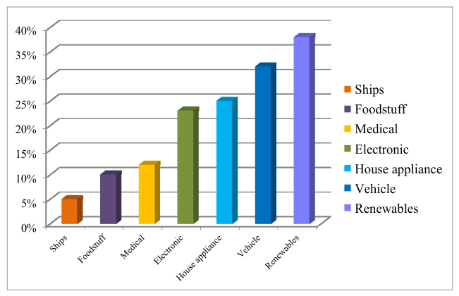
Figure 1. The proportion of 5G network applications deployed in various industries.
Applsci 16 05223 g001
Figure 2. Communication topology for industrial private networks.
Applsci 16 05223 g002
Figure 3. Axially Aligned Bounding Box.
Applsci 16 05223 g003
Figure 4. Algorithm flowchart.
Applsci 16 05223 g004
Figure 5. Simulation results under different numbers of fixed terminals.
Applsci 16 05223 g005
Figure 6. Simulation results under different numbers of dynamic terminals.
Applsci 16 05223 g006
Figure 7. Optimal AP deployment location heatmap.
Applsci 16 05223 g007
Figure 8. Results of site validation obtained with an R&S signal analyzer.
Applsci 16 05223 g008
Table 1. Experimental configuration parameters.
ParametersValue
The transmission power P A of AP20 dBm
Path loss coefficient γ 2.4
The actual signal strength received at the reference point P L ( d 0 ) 40 dB
The minimum receiving level of the terminal P 0 −75 dBm
The initial solution generates the matrix scaling coefficient N d 4
The side lengths d of the small cube blocks that divide the space0.5 m
The size of the solution set in Algorithm 460
The maximum number of iterations in Algorithm 4100
The probability p of conducting a large-scale search in Algorithm 450%
The weight ks of signal distribution uniformity on the path of mobile terminals0.2
Table 2. The measurement result.
Point IDPosition (x,y,z)LoS/NLoSPredicted RSRP (dBm)Measured RSRP (dBm)Error (dB)Measured EVM (%)
P1(10,15,1.5)LoS−45.2−43.81.42.14
P2(25,30,1.5)LoS−62.7−63.81.11.62
P3(8,2,4)NLoS−39.6−41.31.82.56
P4(2,10,5)LoS−42.3−43.61.32.43
Table 3. The parameters used in the experiments of this section.
AlgorithmNumber of Weak Signal BlocksPercent of Weak Signal BlocksThe Sum of the Standard Deviations of the Signal Strength
The proposed method967.82%50.4
Genetic algorithm1109.33%66.5
Uniform deployment18915.28%70.2
Table 4. Power consumption of the APs.
APAssociated TerminalsThroughput Load (Mbps)Required Tx Power (dBm)Total Power (kW)
AP 1F1, F2, M2, M3, M48555.66.3
AP 2F3, F5, F6, M5~M109542.85.8
AP 3F7, F86038.75.2
AP 4F9, F105030.44.3
Total 290167.521.6
Table 5. Comparison with existing deployment optimization methods.
FeatureProposedRef. [36]Ref. [37]Ref. [38]
Mixed terminal types
Mobile terminal paths
Heat map pre-computation
Industrial obstacle modeling
Power capacity estimation
Disclaimer/Publisher’s Note: The statements, opinions and data contained in all publications are solely those of the individual author(s) and contributor(s) and not of MDPI and/or the editor(s). MDPI and/or the editor(s) disclaim responsibility for any injury to people or property resulting from any ideas, methods, instructions or products referred to in the content.