An Ab Initio Molecular Dynamics Study of Key Thermodynamic Input Parameters for Computer Simulation of U-6Nb Solidification

Abstract

The key to metallic fuel development is the fabrication of uranium metal and alloys into fuel forms. U-Nb alloys are one of the best candidates for a metallic fuel alloy with high-temperature strength sufficient to support the core, acceptable nuclear properties, good fabricability, and compatibility with usable coolant media. Melt processing has been a key component of the metallic fuel cycle, and process models require thermophysical parameters at elevated temperatures, particularly above the melting temperatures, regarding which experimental data are scarce, for accurate simulations and process development. By means of ab initio density-functional theory (DFT) quantum molecular dynamics (QMD), we have calculated the main thermophysical parameters—the density, thermal expansion coefficient, specific heat, thermal conductivity, melting temperature, latent heat of fusion, and viscosity—used in the modeling of the U-6 wt.% Nb alloy casting. The melting temperature of the U-6 wt.% Nb alloy at ambient pressure is obtained by means of QMD simulations using the Z-method. The ambient volume change and latent heat of melting of U-6 wt.% Nb are also derived from QMD simulations in conjunction with analytical fitting for the energy and pressure. The thermal conductivity for the solid U-Nb alloy is calculated from the semi-classical Boltzmann transport equation combined with an estimate of the electron relaxation time obtained from DFT simulations.

1. Introduction

The main goal of fast breeder reactors is to achieve high burn-up, which involves fissioning all types of transuranic elements, thereby providing an appropriate solution to spent fuel recycling and ensuring the complete transmutation of long-lived minor actinides (Np, Am, and Cm). This defines a closed nuclear fuel cycle with future disposition of the nuclear waste products in a single geological repository [1,2,3]. Metallic nuclear fuels are ideal because of their high density and high thermal conductivity, relative to oxide fuels. However, the relatively low melting temperatures of U and Pu alloys make them unsuitable for high-temperature applications. To increase the solidus temperature of U-Pu alloys, the addition of Mo [4,5], Nb [6,7], Zr [8,9], and Ti [10,11] is commonly used.

In pure uranium metal, the body-centered-cubic (BCC) allotrope, γ, is only stable at elevated temperatures (776 °C < T < 1135 °C) [12,13]. On cooling, uranium undergoes a solid–solid phase transformation to the tetragonal β phase (observed in a very small interval of temperatures and pressures), followed by a second transformation to the orthorhombic α phase, which is stable at room temperature and below. Among these phases, γ phase has the most suitable properties for nuclear engineering purposes, due to its cubic symmetry, isotropy, and elastic properties. However, γ-uranium is known to stabilize at high temperatures by phonon–phonon coupling that is strongly anharmonic [14]. Consequently, this phase is decidedly unstable at low temperatures (T < 776 °C) and quenching cannot suppress spontaneous transformation to non-cubic crystal structures.

Uranium metal at low temperatures, where machining and other material processing may take place, exists in the α-uranium structure, which is less than ideal due to its brittle nature, poor corrosion resistance, and proneness to oxidation. The poor corrosion res istance and undesirable combinations of strength and ductility observed in this phase have spurred numerous investigations into methods to destabilize this phase by introducing one or more alloying constituents. Alloying α-U with Nb [15,16,17] is a common method to effectively improve the mechanical properties and corrosion resistance. The addition of Nb significantly increases the oxidation resistance of U, because Nb is distributed uniformly in the U matrix [18].

The equilibrium U-Nb phase diagram has been presented and discussed in numerous papers [19,20,21,22,23,24]. There is a complete solubility across the equilibrium U-Nb phase diagram in the high-temperature γ-phase but below the critical temperature, T_c = 950 ± 20 °C, the uranium–niobium phase diagram displays a γ-phase miscibility gap (γ(BCC) → γ₁(BCC) + γ₂(BCC)) with decomposition of the γ₁-phase according to the monotectoid reaction γ₁ → γ₂ + α at 647 °C [19,21], where the γ₁ and γ₂ phases contain 13.3 at.% and 70 ± 2 at.% Nb, respectively, while the α phase has less than 1 at.% Nb in solution. Because this scenario represents the equilibrium U-Nb phase diagram, the decomposition of the γ₁ is diffusional, forming a two-phase structure with unalloyed α uranium and the niobium-rich γ₂-phase. The resulting mixture suffers degraded corrosion resistance and ductility [15,16,17,24,25,26,27] due to the lack of niobium in solid solution.

Among Mo, Nb, Zr, and Ti, only Nb does not form stoichiometric compounds with U; however, U-Nb alloys have three metastable phases: γ⁰ (tetragonal), α” (monoclinic), and α’ (orthorhombic), whose formation depends on Nb concentration in U-Nb alloys during rapid quenching. For instance, the Nb supersaturated γ phase undergoes a transition to α’ structure at Nb contents (0–4.2 wt.%), to α” structure at Nb contents (4.2–6.9 wt.%), and to γ⁰ structure at higher Nb contents (6.9–8.9 wt.%) [7,20,21]. The exact composition of U-6Nb alloy (U-6 wt.% Nb, or U-14.06 at.% Nb) originates from the position (at 6 wt.% Nb) of the monotectoid point in the U-Nb phase diagram at T = 647 °C where the monotectoid reaction γ₁ → γ₂ + α starts (see Figure 1 from Ref. [19] or Figure 3.7 from Ref. [21]). U-6Nb alloy remains stable at the BCC structure (γ-phase) at T ≥ 600 °C. However, as the alloy is cooled down rapidly to room temperature, it undergoes a two-stage transformation process: at T∼570 °C, the material exhibits transformation into the metastable γ₀ phase. At a lower temperature of ∼370–450 °C, the alloy undergoes further transformation into the metastable α” phase. With an Nb concentration of ∼60 to 100 wt.%, the U-Nb system forms a continuous solid solution of the BCC (γ) structure in the entire temperature range [19].

Djurič [28], relating to Cahn’s theoretical argument [29], mentioned that during the monotectoid decomposition described above, the equilibrium composition of the product phases could only be achieved in the ideal case when the reaction rate approaches zero. Based on the mechanism suggested by Djurič [28], Zhang et al. [30] and Duong et al. [24] concluded that the phase transition from the high-temperature γ-phase to the low-temperature equilibrium α-uranium and niobium-rich γ₂-phase occurs through metastable (quenched) phases: γ⁰, α”, and α’. The reactions producing α” and γ⁰ phases are generally regarded as martensitic (diffusionless) in nature, occurring by shear and/or displacive mechanisms that require only cooperative, short-range motions of the atoms [17]. The Nb supersaturated metastable α”-phase solid solution exhibits far better corrosion resistance than unalloyed uranium. It is also amenable to subsequent age hardening, which promotes a wide range of mechanical properties [31,32,33,34,35,36,37,38,39,40] through the selection of aging temperature and time [21,34].

From a modeling standpoint, there are fewer studies mostly from the phenomenological works reported [23,24,41,42,43,44,45,46]. Uranium–niobium has also been investigated from first-principles electronic-structure theory [47,48,49,50,51,52,53,54,55,56,57,58].

The key to metallic fuel development is the fabrication of uranium metal and alloys into fuel forms. Casting (the process in which a liquid metal is poured into a mold [59,60,61,62]) and other melt processing methods are key components of the metallic fuel cycle, and modeling these processes can increase the reliability of producing sound parts. However, process modeling requires thermophysical parameters at elevated temperatures, particularly above the melting temperature, for which experimental data are scarce. The main thermophysical parameters needed are the density, thermal volume expansion, specific heat, thermal conductivity, melting temperature, latent heat of fusion, and viscosity, each property affecting the process in a specific manner.

The liquid metal density is used to calculate the total mass of metal needed to fill the mold volume and is also used for defect/porosity prediction. Liquid metal density governs the hydrostatic pressure, which influences mold design and the gating system, and controls the degree of shrinkage during cooling and solidification of the melt.

The solid thermal volume expansion plays a primary significance in the cooling and solidification of the melt, especially affecting dimensional accuracy, predicting how much the metal will expand when heated and contract when cooling. An accurate thermal expansion coefficient helps to estimate total shrinkage from liquid to room temperature, so that patterns and molds can be designed with proper allowance for dimensionally accurate parts. The knowledge of the thermal expansion coefficient also helps in the selection of the mold material, which should accommodate expansion/contraction without causing cracks or distortion.

The specific heat is the critical parameter of melt processing because it defines how much energy is needed to raise the temperature necessary to melt and superheat the metallic alloy. In melt processing, the total heat that must be removed from the molten metal to reach its solidification temperature is directly proportional to its specific heat, the temperature differential, and mass. The specific heat of both the alloy and mold material is a key factor that must be controlled and accounted for to manage the microstructure and control the location of defects. A higher specific heat requires a longer time for the mold to extract the heat, resulting in a slower cooling rate and longer solidification time. A slower cooling rate often leads to a coarser grain structure in the final solidified metal. The coarser grain structure can influence the mechanical properties, generally leading to lower strength and ductility relative to a finer grain structure.

The thermal conductivity is also critical in melt processing because it defines the rate of heat transfer inside a material, directly affecting the cooling rate of the metal as the metal solidifies. During casting, heat flows from the hot liquid metal into the cooler mold. The rate and uniformity of this heat flow depends on the thermal conductivity of both the metal and mold. High thermal conductivity causes rapid heat transfer and thus quicker solidification, which can refine the grain structure and improve mechanical properties. Slow heat transfer can cause hot spots leading to shrinkage cavities, porosities, or cracks.

The melting temperature determines the minimum (pouring) temperature at which the metal must be heated for casting. The mold material should be selected accordingly to withstand the required temperature. The melting temperature partially affects the solidification control (the cooling rate and solidification process), impacting grain structure.

The latent heat of fusion is used to calculate the total energy required to melt the metal from solid to liquid. The latent heat of fusion influences how much energy must be removed from the metal to solidify and thus affects the cooling system design. The precise knowledge of the latent heat of fusion is important for designing both the heating and cooling systems for any melt processing.

The viscosity of the liquid metal is a key factor in designing the size and shape of gates and runners to ensure proper metal flow. Viscosity determines how easily the liquid metal flows through the gating and mold system and how easily convection and other flows can mix and homogenize a melt. For example, high viscosity can cause incomplete filling or defects. However, high viscosity can also reduce defects due to turbulence and air entrapment. At the same time, viscosity affects the optimal pouring speed, e.g., low viscosity field of the melt, temperature, and time.

According to references [59,62], the fundamental requirement for any model that can simulate casting processes is the solution of the heat flow equation in the metal and the mold. The input parameters of this equation are density, specific heat, thermal conductivity, the latent heat of fusion, the velocity field of the melt, temperature, and time.

To simulate this filling procedure, the Navier–Stokes equation together with the mass conservation equation must be solved [59]. In addition to density, velocity of the melt, and pressure, the knowledge of the kinetic viscosity is necessary. The thermal expansion coefficient and volume change on solidification are necessary to simulate stress and distortion due to solidification [59,62].

Contamination and the swift oxidation of the melt present further challenges to the measurement of the required values. These complications introduce ambiguity into the measurements and frequently exert unanticipated effects on the recorded values. Consequently, possessing thermophysical data devoid of these influences is highly advantageous. The calculations performed in this work are a step toward reducing the uncertainty in these values by avoiding some of these experimental complications.

This study conducted DFT quantum molecular dynamics (QMD) simulations of liquid U-6Nb alloys within a temperature range of 1400 K to 2600 K, incremented by 200 K. The equilibrium volume is determined by modifying the lattice constant to the value that aligns with the external pressure near zero at the specified temperature. The determined equilibrium volume is utilized to establish the density of the melt at the specified temperature. The specific heat is defined as the variation in the system’s enthalpy relative to a change in temperature, with pressure held constant. The computed mean-square displacement over time determines the diffusion coefficient and viscosity of the melt. The melting temperature is determined using the Z-method. The electron thermal conductivity is ultimately derived from the calculation of the electron relaxation time.

Computational details of the present calculations are outlined in Section 2, followed by a presentation of the results of the density, thermal expansion, and specific heat in Section 3. The results of the melting temperature and latent heat of fusion are presented in Section 4. Section 5 shows the results of calculations of self-diffusion coefficients and viscosity. Section 6 presents the results of calculations of thermal conductivity. Lastly, a summary and concluding remarks are outlined in Section 7.

2. Computational Methodology

2.1. Ab Initio Molecular Dynamics

Within the framework of the density-functional theory (DFT) we perform QMD simulations using the projector augmented wave (PAW) method [63] as implemented in the Vienna ab initio simulation package (VASP) [64,65,66,67]. The electronic structure of U is represented by [Xe4f¹⁴5d¹⁰] 5f³6s² 6p⁶ 6d¹ 7s² (14 valence electrons), while that of Nb is represented by [Ar 3d¹⁰]4s²4p⁶4d⁴5s¹ (13 valence electrons). For the electron exchange and correlation functionals, the Perdew–Burke–Ernzerhof (PBE) implementation of generalized gradient approximation (GGA) is used [68], and the cutoff energy on the plane-wave basis expansion is selected as 300 eV for both U and Nb. We use the Fermi–Dirac smearing method [69], where the parameter σ acts as the electronic temperature (σ = k_BT) when simulating electronic temperature.

In order to perform simulation of γ-U-6Nb alloy, we construct a 128-atom (4 × 4 × 4) supercell with the periodic boundary conditions and a single Γ-point to sample the Brillouin zone of the supercell. The choice of a single Γ-point is equivalent to that in [51] and is completely justified by the results of our convergence tests with respect to the density of k-point mesh, from comparing results of several of our simulations using a single Γ-point to those with 2 × 2 × 2 and 3 × 3 × 3 k-point meshes and system size, from comparing our results for a 128-atom system to those for a 250-atom system from our previous study [70]. Comparison with the 250-atom system can be found in the Section 7. A 128-atoms supercell contains randomly distributed 111 atoms of U and 17 atoms of Nb that results in an Nb composition of ~13.28 at.%. As was mentioned in the Introduction, U-6 wt.% Nb corresponds to U-14.06 at.% Nb, so our choice corresponds to a slightly lower weight % of Nb. In our modeling we use the U_86.72Nb_13.28 128-atoms computational cell that resembles the U_86.23Nb_13.77 alloy studied in [35,52]. In order to calculate the equilibrium volume, density, thermal expansion coefficient, and specific heat, we perform QMD simulation using the canonical NVT ensemble where the number of atoms, N, volume, V, and temperature, T, are kept constant with the Nose–Hoover thermostat [71,72], and the velocity-Verlet algorithm [73,74,75] is used to integrate the Newton’s equation of motion with a time step of 3 fs which is the same as was used in Ref. [51]. Note that, as shown in [76], for a system of heavier constituents like U, the choice of 3 fs is fully justified, and the accuracy of the results of simulations is like that of the simulations of hydrogen using 1 fs, albeit at a much lower computational cost.

In our NVT calculations we follow the methodology suggested by Shi et al. [51] and apply it to the U₁₁₆Nb₁₂ (U_90.625Nb_9.375) liquid alloy. Using VASP formalism and the Voronoi tessellation, the authors [51] studied the evolution of the local atomic structure (chemical short-range order) of the U_90.625Nb_9.375 alloy during solidification.

An NVT simulation is conducted at T = 2600 K for a total duration of 32,000 time steps, equating to 96 ps. As in Ref. [51], we initiate calculations using a γ-U (BCC) structure with a computational cell comprising 128 atoms, characterized by an initial lattice constant of a₀ = 3.475 Å (per unit cell) or A₀ = 13.9 Å (per computational 4 × 4 × 4 cell). Furthermore, analogous to Ref. [51], we presume that the lattice constant of the computational cell, A₀ = 13.9 Å, is applicable at the temperature T = 0 K.

In these simulations, we adjust the lattice constant of the computational cell to simulate ambient pressure. We commence with the initial configuration, A₀ = 13.9 Å, and conduct a sequence of QMD calculations comprising 17,000 steps (51 ps) until achieving a stable thermal equilibrium at T = 2600 K. Our analysis of the radial distribution functions (RDF), see Section 3, revealed that the computational system completely melts at T = 2600 K.

In the next five consecutive computational runs, each lasting 3000 steps (9 ps), we employ the final configuration obtained from the initial 17,000 QMD steps as the starting configuration. These five computational simulations enable us to determine the optimal value of the equilibrium lattice constant (volume) at ambient pressure, p = 0. The total energy and external pressure are determined through statistical analysis (averaging) during each computational run.

Starting from the final configuration obtained at T = 2600 K, we perform QMD simulations at 2400 K (84 ps), 2200 K (108 ps), 2000 K (72 ps), 1800 K (63 ps), 1600 K (108 ps), and 1400 K (80 ps). These results are also shown in Section 3.

To calculate the melting temperature of U-6Nb alloy we used the Z-method implemented in VASP. The Z-method is a procedure used to calculate the melting curves of materials by modeling a solid system at different initial total energies [77,78]. A solid system is modeled in a microcanonical NVE ensemble, where N is the number of atoms, V is the volume, and E is the total energy of the system.

It has been observed that if a crystal melts homogeneously, it can be overheated substantially above its melting temperature, T_m. However, there is a critical T_LS above which one cannot heat a solid without transforming it into a liquid structure. Also, even though superheating is a comparatively rare phenomenon in nature, it could be easily simulated because a perfect crystal with periodic boundary conditions (PBC) is simulated in typical molecular dynamics runs. A perfect crystal with PBC has no surfaces, which are required to avoid superheating. Therefore, atomistic simulations without an interface are perfectly suited to study homogeneous melting.

When we heat the crystal at a constant volume, the pressure, p, increases with temperature, T. When temperature, T, approaches T_LS, a very small increase in the initial kinetic energy leads to melting, and T will drop to T_m at P = P_m, where p is the external pressure. In other words, at each selected volume, V, the system can transit from the superheated solid state to the liquid state at constant energy: E_S(T_L;V) = E_L(T_m;V).

In each simulation, E is controlled by the corresponding choice of the initial temperature T_S. The shape of the P-T trajectory mapped out by the final states of simulations with different initial Ts resembles the letter Z, which is the origin of the method’s name. The Z-method has been used in numerous studies of melting curves, e.g., Pb [79], Mo [80], Fe and Fe_0.9375Si_0.0625 [81], MgO [82], Ta [83,84], Pt [84,85,86], ZrO₂ [87], Os [88], Zn [89], Si [90], CaSiO₃ [91], C [92], Sn [93], Ag [94], Cu [95], Co [96], SiO₂ [97].

NVE QMD simulations are performed for 7 temperatures: 2500 K, 2750 K, 3000 K, 3225 K, 3500 K, 3750 K, and 4000 K with a duration of 42 ps, each.

Our total simulation times (lengths) are long enough to ensure that the averaging of the equilibrated quantities such as melting temperature and pressure in the Z-method simulations or pressure in the NVT and NVE simulations brings up the corresponding values with errors of a fraction of a percent.

2.2. Self-Diffusion Coefficient and Viscosity

We also calculated the self-diffusion coefficient for the liquid U₁₁₁Nb₁₇ alloy through the Einstein relation [98]:

$$D = \underset{t\to \infty }{\mathit{lim}}{\displaystyle \frac{<∆r^2\left(t\right)>}{6t}},$$

(1)

where

$${<r}^2\left(t\right)>={\displaystyle \frac{1}{N}}{\sum }_{i=1}^N{\left[r_i\left(t+t_0\right)-r_i\left(t_0\right)\right]}^2$$

(2)

is the atomic mean-square displacement (MSD). We calculate the mean-square displacement from QMD runs by integrating Newton’s equation of motion with a time step of 1 fs performing 6000 QMD steps with the total duration of 6 ps.

The viscosity, η, is calculated through the modified or generalized Stokes–Einstein relation [98]:

$$\eta = {\displaystyle \frac{k_B T}{2\pi Da}},$$

(3)

where D is the self-diffusion coefficient, T is temperature, and a is the affective atomic diameter. One should mention the classical Stokes–Einstein relation [99]:

$$\eta = {\displaystyle \frac{k_B T}{6\pi D{r}_i}}= {\displaystyle \frac{k_B T}{3\pi Da}},$$

(4)

where r_i is the effective atomic radius of a spherical particle, which is derived for a macroscopic sphere in a continuum fluid. For atomic diffusion in a dense metallic liquid, this hydrodynamic picture is not valid, and the effective friction coefficient differs. Indeed, the friction coefficient depends on the interface condition between particle and solvent, reflecting how the fluid velocity behaves at the surface of a moving particle [100]. A modified Stokes–Einstein relation (3) is often used, where the semi-empirical factor 2π reflects a different friction model suitable for atoms in metals [100,101].

2.3. Thermal Conductivity

Thermal conductivity is challenging to evaluate for liquids, particularly U–Nb melts, due to the lack of long-lived phonon quasiparticles and the complex interplay of ionic and electronic scattering. As a proxy system with well-defined quasiparticle states, we consider the ordered BCC γ-phase compound γ-U₇Nb (7 atoms of uranium and one atom of Nb). The computational cell contains 28 atoms of uranium and 4 atoms of niobium. The total thermal conductivity is decomposed as [102]:

κ(T) = κ_e(T) + κ_ℓ(T),

(5)

where κ_e and κ_ℓ denote the electronic and lattice (phonon) contributions, respectively. We will focus next on electronic contribution.

2.3.1. Boltzmann Transport Formalism

The electronic transport coefficients were evaluated using semiclassical Boltzmann transport theory within the relaxation time approximation (RTA), as implemented in BoltzTraP2 [103]. The method uses Kohn–Sham band energies ${ℇ}_{n\overline{k}}$ (band index n, wave vector $\overline{k}$) obtained from density-functional theory (DFT) calculations (VASP) [66,67]. For each state, the group velocity is

$${\overline{v}}_{n\overline{k}}={\displaystyle \frac{1}{ђ}}{▽}_{\overline{k}}{\epsilon }_{n\overline{k}}$$

(6)

Under weak driving forces (electric field $\overline{E}$ and temperature gradient $\overline{▽}$T), the steady-state Boltzmann equation can be linearized about the Fermi–Dirac distribution:

$$f^0(\epsilon , \mu , T) = {\left[1+exp\left({\displaystyle \frac{ϵ-\mu }{k_{B}T}}\right)\right]}^{-1},$$

(7)

where μ is the chemical potential and k_B is the Boltzmann constant. Within the RTA, the deviation $\delta f_{n\overline{k}}$ = $f_{n\overline{k}}- f^0$ takes the form

$$\delta f_{n\overline{k}}={\tau }_{n\overline{k}}\left(-{\displaystyle \frac{\delta f^0}{\delta \epsilon }}\right){\overline{v}}_{n\overline{k}}•\left[q\overline{E}+{\displaystyle \frac{{\epsilon }_{n\overline{k}}-\mu }{T}}\left(-\overline{▽}T\right)\right],$$

(8)

where q is the carrier charge (q = − e for electrons) and ${\tau }_{n\overline{k}}$ is the state-dependent relaxation time.

The charge-current density $\overline{J_e}$ and heat-current density $\overline{J_Q}$ follow from

$$\overline{J_e}=q{\sum }_n{\int }_{BZ}{\displaystyle \frac{d\overline{k}}{{\left(2\pi \right)}^3}}{\overline{v}}_{n\overline{k}}\delta f_{n\overline{k}};\overline{J_Q}={\sum }_n{\int }_{BZ}{\displaystyle \frac{d\overline{k}}{{\left(2\pi \right)}^3}}\left({\epsilon }_{n\overline{k}}-\mu \right){\overline{v}}_{n\overline{k}}\delta f_{n\overline{k}}.$$

(9)

It is convenient to introduce generalized transport moments (second-rank tensors):

$${\mathcal{L}}_{\mathit{i}\mathit{j}}^{\left(\mathit{m}\right)}\left(\mu ,T\right)={\displaystyle \frac{1}{\mathsf{\Omega }}}\sum _n{\int }_{BZ}{\displaystyle \frac{d\overline{k}}{{\left(2\pi \right)}^3}}{\tau }_{n\overline{k}}{v}_{i,n\overline{k}}{v}_{j,n\overline{k}}{\left({\epsilon }_{n\overline{k}}-\mu \right)}^m\left(-{\displaystyle \frac{\delta f^0}{\delta \epsilon }}\right),$$

(10)

where Ω is the unit-cell volume and i, j denote Cartesian directions.

From Equation (10), the electrical conductivity tensor is

$${\sigma }_{ij}\left(T\right)=q^2{\mathcal{L}}_{\mathit{i}\mathit{j}}^{\left(\mathbf{0}\right)}.$$

(11)

The Seebeck tensor is:

$$S_{ij }\left(T\right)= {\displaystyle \frac{1}{qT}}{\left({\mathcal{L}}^{\left(0\right)}\right)}_{i,k}^{-1}{\mathcal{L}}_{kj}^{\left(1\right)},$$

(12)

and the electronic thermal conductivity tensor under open-circuit conditions ($\overline{J_e}$ = 0) is

$${\kappa }_{e, ij}\left(T\right)={\displaystyle \frac{1}{T}}\left[{\mathcal{L}}_{ij}^{\left(2\right)}-{\mathcal{L}}_{ik}^{\left(1\right)}{\left({\mathcal{L}}^{\left(0\right)}\right)}_{kl}^{-1}{\mathcal{L}}_{lj}^{\left(1\right)}\right]$$

(13)

For the cubic BCC phase, the diagonal components are equivalent, and we report the scalar value

$${\kappa }_e\left(T\right)={\displaystyle \frac{1}{3}}\mathrm{T}\mathrm{r}[\stackrel{═}{{\kappa }_e\left(T\right)}]$$

(14)

(and similarly, for σ and S).

2.3.2. Constant Relaxation Time Approximation and Scaling

In the constant relaxation time approximation (CRTA), ${\tau }_{n\overline{k}}$ = τ and Equations (11)–(13) yield σ ∞ τ and κ_e ∞ τ, whereas S is independent of τ. Accordingly, BoltzTraP2 provides transport coefficients up to an overall multiplicative factor set by τ [103]. Absolute values were obtained using an electronic relaxation time obtained independently from VASP transport and electron–phonon scattering calculations:

τ = 1.2 × 10⁻¹⁵ s.

(15)

2.3.3. Electronic-Structure Calculations and Volume Mapping

The DFT eigenenergies ${ℇ}_{n\overline{k}}$ were calculated for γ-U₇Nb at seven lattice constants. To facilitate comparison with liquid-state simulations, the lattice constants were chosen to represent the liquid-like volumes at T = 1400, 1600, 1800, 2000, 2200, 2400, and 2600 K. Each lattice constant defines a distinct electronic structure and corresponding ${\kappa }_e\left(T\right)$ through Equations (10)–(14). Next, we consider the lattice contribution to thermal conductivity.

2.3.4. Estimate of the Lattice Contribution

The lattice contribution, κ_ℓ(T), is expected to be much smaller than κ_e(T) for this metallic system. We estimate κ_ℓ(T) using temperature-dependent phonon information for unalloyed γ-U from Ref. [104] combined with a classical kinetic expression [105].

$${\kappa }_l\left(T\right)\approx {\displaystyle \frac{1}{3}}{C}_v\left(T\right)v_s^2\left(T\right){\tau }_{ph.}\left(T\right)\mathrm{or} {\kappa }_l\left(T\right)\approx {\displaystyle \frac{1}{3}}{C}_v\left(T\right)v_s\left(T\right)l\left(T\right)$$

(16)

where C_v is the phonon specific heat, v_s is a characteristic sound velocity, and τ_ph.(or l) is the phonon lifetime (or mean free path). Specifically, one requires the temperature dependence of the elastic constants C₁₁, C₁₂, and C₄₄. These moduli are in turn obtained from the temperature-dependent phonon dispersions from the slope of these approaching the Γ point. For these calculations, we did include spin–orbit coupling because this effect is subtly helping to stabilize the BCC γ phase; see more details in Ref. [104].

3. Density, Specific Heat, Thermal Expansion of Liquid U-6Nb Alloy

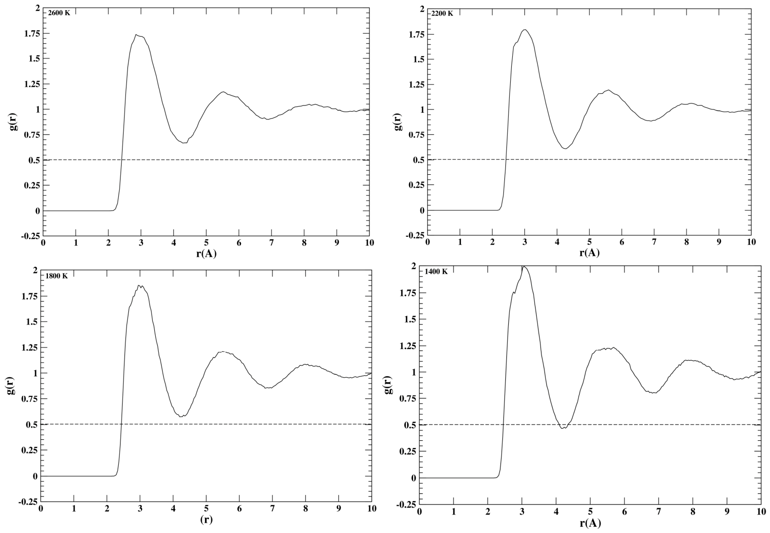
Figure 1 shows the calculated (NVT ensemble) radial distribution functions (RDF) of the U₁₁₁Nb₁₇ alloy at 2600 K, 2200 K, 1800 K, and 1400 K, respectively. The first three radial RDFs exhibit the characteristic features of the liquid: the height of the RDF first peak is less than 2, and the depth of the first minimum of RDF is less than 0.5 (see Appendix A). Also, two main peaks clearly exist between 2.4 and 4.3 Å and 4.3 and 6.8 Å. At T = 1400 K the height of the first maximum of RDF is equal to 2, but the depth of the first minimum of RDF is larger than 0.5. According to the calculation, discussed in the next Section, melting temperature of the U₁₁₁Nb₁₇ alloy, we consider that RDF at = 1400 K represents the supercooled liquid (the second peak is broadened).

Calculated equilibrium atomic volume and density of the U₁₁₁Nb₁₇ alloy at different temperatures are presented in

Table 1. Atomic volume, density, and relative thermal expansion coefficient of the U_86.72Nb_13.28 alloy at different temperatures. The experimental density of pure liquid uranium, ρ_U, is also presented in the last column. * Note that the density of liquid uranium is measured at the experimental melting point, $T_m^U$ = 1408 K.

T (K)	Ω0 (Å3)	ρ (g/cm3)	α (%)	ρU (g/cm3) [106,107]
1400	21.746	16.705	3.6442	17.23 *
1600	21.984	16.524	4.7785	16.88
1800	22.192	16.369	5.7699	16.53
2000	22.436	16.191	6.9328	16.18
2200	22.650	16.038	7.9528	-
2400	22.888	15.871	9.0871	-
2500	-	-	-	15.33
2600	23.154	15.689	10.3549	-

. This table also presents calculated values of the relative thermal expansion coefficient (not to be confused with isobaric thermal expansion coefficient α_P considered in what follows) calculated by the equation:

$$\alpha = {\displaystyle \frac{{{\Omega }_0}_T - {{\Omega }_0}_0}{{{\Omega }_0}_0}},$$

(17)

where ${{\mathit{\Omega }}_{\mathbf{0}}}_{\mathbf{0}}$ corresponds to the initial atomic volume of the 4 × 4 × 4 cell of γ-U with the lattice constant a₀ = 3.475 Å [51]. ${{\mathit{\Omega }}_{\mathbf{0}}}_{\mathbf{0}}=\mathbf{0.5}{\mathit{a}}_{\mathbf{0}}^{\mathbf{3}}\approx \mathbf{20.9814} {\mathit{Å}}^{\mathbf{3}}$ at T₀ = 0 K and ${{\mathit{\Omega }}_{\mathbf{0}}}_{\mathit{T}}$ is the calculated atomic equilibrium volume at a given temperature T.

There are no experimental data on the density of the liquid U_1-xNb_x alloys. That is why we compared the results of our calculations with the experimental density of pure liquid uranium [106,107] that is also presented in Table 1. At T = 1400 K the difference between densities of the U₁₁₁Nb₁₇ and uranium melts is about 3%; however, at T = 2000 K these densities are almost equal.

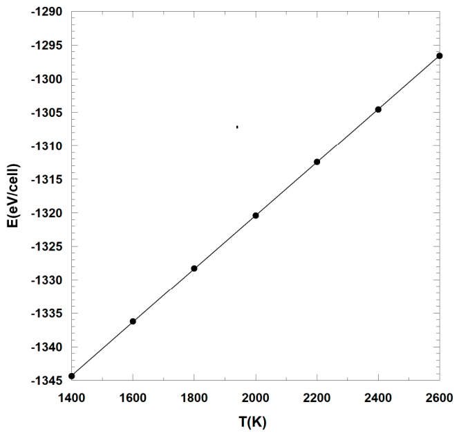
Figure 2 shows the temperature dependence of the potential energy of the U₁₁₁Nb₁₇ alloy.

Using the expression $C_p={\left({\displaystyle \frac{\partial H}{\partial T}}\right)}_{p,N}= {\left({\displaystyle \frac{\partial E}{\partial T}}\right)}_{p,N}$, we calculated the potential energy contribution to the specific heat $C_p^{ potential}\left(T\right)=0.039748 {\displaystyle \frac{eV}{\left(cell \times K\right)}}=29.961776{\displaystyle \frac{J}{\left(mol \times K\right)}}$ that does not change with temperature. The kinetic energy contribution to the specific heat is equal to $C_p^{kinetic}= {\displaystyle \frac{3}{2}}R=12.471693{\displaystyle \frac{J}{\left(mol \times K\right)}}$, where $R=8.314462{\displaystyle \frac{J}{\left(mol \times K\right)}}$ is the molar gas constant. This, the specific heat under constant pressure of the U₁₁₁Nb₁₇ alloy is equal to $C_p\left(T\right)=$ $C_p^{ potential}\left(T\right)+ C_p^{kinetic}=42.433469 {\displaystyle \frac{J}{\left(mol\times K\right)}}$ and does not change with temperature.

Like in the case with density, there are no measurements of the specific heat of the U₁₁₁Nb₁₇ liquid alloy. There are few measurements of the specific heat of liquid uranium. According to [108,109,110], the specific heat of liquid uranium metal does not change with temperature that is in accord with our calculations for the U₁₁₁Nb₁₇ liquid alloy.

4. Melting of U-6Nb Alloy

4.1. Melting Temperature Calculation

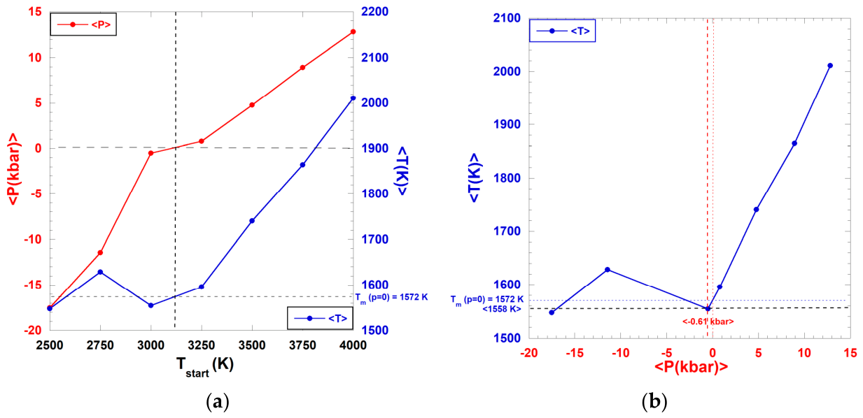
Figure 3 presents the outcomes of NVE calculations for the U₁₁₁Nb₁₇ alloy conducted at the equilibrium atomic volume of T = 1600 K, with Ω₀ = 21.984 ų (a ≈ 3.5295 Å). Calculations are conducted for seven initial temperatures, T_start, as outlined in the Introduction. Figure 3a illustrates the averaged pressure <P> and temperature <T> obtained from each calculation. The Z-methodology indicates that each calculation determines the melting temperature of the U₁₁₁Nb₁₇ alloy at specific pressures illustrated in Figure 3a. The dashed lines indicate that at ambient pressure, <P> = 0 kbar, the melting temperature of the U₁₁₁Nb₁₇ alloy is T_m = 1572 K, which aligns closely with the melting temperature T_m = 1577 K calculated in Ref. [70] for the 250-atom U₂₁₅Nb₃₅ computational cell. Figure 3b illustrates the correlation between pressure and temperature along the isochore associated with the volume of the bcc lattice, Ω₀ = 21.984 ų (a ≈ 3.5295 Å).

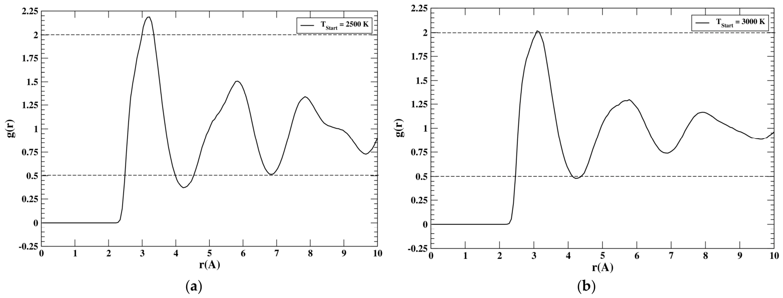
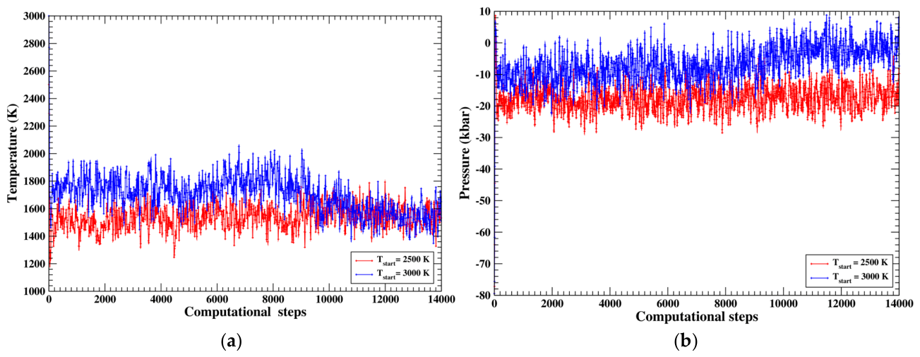
Figure 4 demonstrates the time evolution of, T and P, respectively, of the U₁₁₁Nb₁₇ alloy during the QMD NVE runs with two initial temperatures T_start = 2500 K and T_start = 3000 K. During the run with the initial temperature T_start = 2500 K the system remains in a superheated solid state (see Figure 5a and Appendix A) after 14,000 computational steps (42 ps). During the run with the initial temperature T_start = 3000 K the system remains in the overheated solid state up to ~9000 computational steps (27 ps) and then starts melting (see Figure 5b and Appendix A); the melting process takes approximately 9 ps (3000 computational steps). During the melting the temperature decreases from ~1800 K (the overheated solid) to ~1558 K.

Consequently, during the run with the initial temperature T_start = 3000 K pressure increases during the melting interval of ~ 9 ps, from ~−10 kbar (the superheated solid) to ~−0.61 kbar. This happens because the melting of the U₁₁₁Nb₁₇ alloy must be accompanied by a volume expansion; however, since our calculations are performed along the isochore (constant volume, Ω₀ = 21.984 ų), such that volume does not change, during melting the pressure increases instead. Moreover, because in an NVE run the total energy E ~ k_BT + PV is conserved, the increase in P and decrease in T are synchronized.

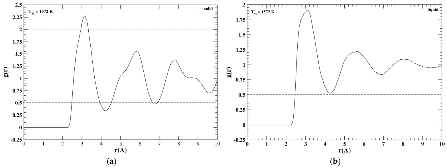
Figure 5 shows RDFs of the U₁₁₁Nb₁₇ alloy calculated at the end (14,000th iteration) of NVE QMD runs with the initial temperatures T_start = 2500 K and T_start = 3000 K. At T_start = 2500 K the height of the first peak of RDF is larger than 2 and the depth of the first minimum of RDF is larger than 0.5 (see Appendix A). Thus, we conclude that NVE QMD with T_start = 2500 K results in the superheated solid that is an accord with our observation based on the time evolution of temperature and pressure during NVE QMD simulations. Contrary, at T_start = 3000 K the height of the first peak of RDF is smaller than 2 and the depth of the first minimum of RDF is smaller than 0.5 (see Appendix A). This confirms our previous conclusion that NVE QMD with T_start = 3000 K results in a liquid state.

It is interesting to compare our value of the ambient T_m of U-6Nb obtained in the DFT-based approach to the one that comes from the machine-learning interatomic potential approach of [111]. In that paper, the solid–liquid phase transition boundary of the U-Nb system is determined, up to an atomic percent of Nb of 30%. Their result for the ambient T_m of pure U is 1286 ± 9 K, which is ~120 K below the actual value of 1408 K from experiment. Assuming that the same difference between the calculated and actual values of T_m holds for U-6Nb as well and taking into account their value of T_m of U-6Nb of ~1450 K, we estimate the actual value of the ambient melting point of U-6Nb to be ~1570 K, in essential agreement with 1572 K from our QMD simulations using the Z-method.

Accuracy of Melting Temperature Calculations Using the Z-Method

The Z-method is widely considered to be very accurate, based on numerous practical applications and close agreement between the melting points calculated using the Z-method and the experimental ones. There exist several alternative methods for the theoretical calculation of the melting points which are analyzed in more detail in [112]. In particular, (i) the heat-until-melt (HUT) method always results in superheating and the corresponding T rather than the true T_m, (ii) the coexistence method always brings up the T of either superheated or supercooled system, because for a solid and liquid juxtaposed in one computational cell a nonzero stress at the solid–liquid interface results in a thermal equilibrium at either slight superheating or supercooling, depending on the sign of the stress or, in other words, whether the liquid–solid volume difference is smaller or larger than the actual one that is never known at the beginning of the coexistence simulations. A useful alternative may be the so-called modified Z-method in which an elongated cell is used, similar to the coexistence simulations, but the simulation procedure itself is essentially the same as for the Z-method. The modified Z-method has been used in several studies, but it has never been demonstrated to outperform the Z-method as regards either the accuracy of the results or the computational cost. Our value of T_m = 1572 K of U-6Nb obtained using the Z-method must be accurate enough because, in addition to being consistent with an independent ML-based calculations mentioned above [111], it is virtually identical to that of our previous work [70] which was shown to be in excellent agreement with the only available experimental studies of the U-Nb system by Rogers, et al. [113] and Drotning [114].

4.2. Latent Heat of Fusion Calculation

4.2.1. General Formalism

The latent heat of fusion is the difference in the values of the enthalpies of liquid and solid at the corresponding melting point (P_m, T_m): L_m ≡ H_ℓ(P_m, T_m) − H_s(P_m, T_m). Since H = E + P V, at ambient P the expression for L_m simplifies to L_m(T_m, P = 0) = E_ℓ(T_m, P = 0) − E_s(T_m, P = 0). In other words, the ambient latent heat of melting is the difference between the total energies of liquid and solid.

VASP allows one to calculate E as a function of the lattice constant a at a given fixed T; in our case T = T_m, the ambient melting point of U-6Nb alloy of T_m = 1572 K. We first obtain P (more specifically, the product of P•Ω₀, where Ω₀ is the atomic volume) as a function of the lattice constant a for both solid and liquid in order to determine the two values of a that correspond to P = 0, namely, a_s and a_l, such that P_s(a_s) = P_l(a_l) = 0. Then, we obtain the two E = E(a) and determine the values of E_s(a_s) and E_l(a_l). Finally, L_m = E_l(a_l) − E_s(a_s).

To carry out the procedure described above in practice, we assume that the thermal EOS of U-6Nb is of the Mie–Grüneisen (MG) form:

$$P(V,T) - P (V,\mathit{0}) = {\displaystyle \frac{\gamma }{V}}(E(V,T) - E(V,\mathit{0})),$$

(18)

with

P(V,T) = P(V,0) + (α_P•B_T) •T, α_P•B_T = const, and E(V,T) = E(V,T) + C_V•T,

(19)

where γ is the Grüneisen parameter, α_P and B_T are, respectively, the corresponding isobaric thermal expansion coefficient at pressure P and the isothermal bulk modulus at temperature T, and (α_P•B_T) is assumed to be independent of either V or T, and C_V is the specific heat at constant V. These two equations lead to γ = α_P •B_T•V/C_V, which is the known thermodynamic relation. As discussed in [70,115], the form of the thermal EOS P(V,T) = P(V,0) + (α_P •B_T)T holds true for many substances and is virtually exact along the corresponding melting curves. The cold (T = 0) counterparts of the thermal EOS satisfy the thermodynamic relation:

$$P(V,0) = - {\left.{\displaystyle \frac{\partial E(V,0)}{\partial V}}\right]}_{T=0}$$

(20)

Therefore, P(V,0) = 0 corresponds to the minimum of E(V,0) as a function of V, i.e., to true T = 0 equilibrium state. However, at T ≠ 0, the zero of P and the minimum of E are shifted from each other. Indeed, as follows from (18) and (19),

$$P(V,T) = - {\left.{\displaystyle \frac{\partial E(V,0)}{\partial V}}\right]}_{T=0}+\left({\alpha }_P{•B}_T\right) T.$$

(21)

Hence at P = 0 but T ≠ 0, the minimum of E = E(V,T) as a function of V corresponds to P = − (α_P •B_T ) T < 0. Considering that α_P •B_T is typically of order 10⁻³, the magnitude of the pressure shift at the minimum of E at the normal melting point of order 10³ K is ~10 kbar.

4.2.2. Fitting the Data Sets of E = E(a) and P = P(a)

When both of the data sets of E = E(a) and P = P (a) as functions of the lattice constant a are available at some fixed T, for example, at the normal melting point, the best fits to those data sets that are thermodynamically consistent via Equations (18)–(21) are found using the following approach. First, we switch from E and P to e = E/N, the total energy per atom, N being the total number of atoms in the supercell used in our simulations, and P$•$Ω₀, Ω₀ = V/N being the atomic volume, which both have the same dimensionality of either eV or kbar ų; the conversion factor is 1 eV = 1602.17662 kbar ų.

We assume that e = e(a) is given by a simple quartic form of $a^{3/2}$:

e(a) = A + Ba^3/2 + Ca³,

(22)

where A, B and C are constants. This choice of e(a) is not theoretically motivated but leads to a relatively simple analytic form of $P•{\mathsf{\Omega }}_0\left(\mathrm{a}\right)$ which is related to e(a) in view of (20), (21). Indeed, it follows, via some algebra, that

$$P•{\mathsf{\Omega }}_0\left(\mathrm{a}\right)=-{\displaystyle \frac{B}{2}} a^{3/2}-\left(C-D\right) a^3,$$

(23)

where D = (α_P •B_T)Tm/2. Thus, the choice (22) leads to (23) and implies the determination of the four constants A, B, C and D. They are determined from the simultaneous fits of the forms, respectively, (22) and (23) to the data sets e = e(a) and P•Ω₀ = P•Ω₀ (a).

4.2.3. The Ambient Volume Change and Latent Heat of Melting of U-6Nb

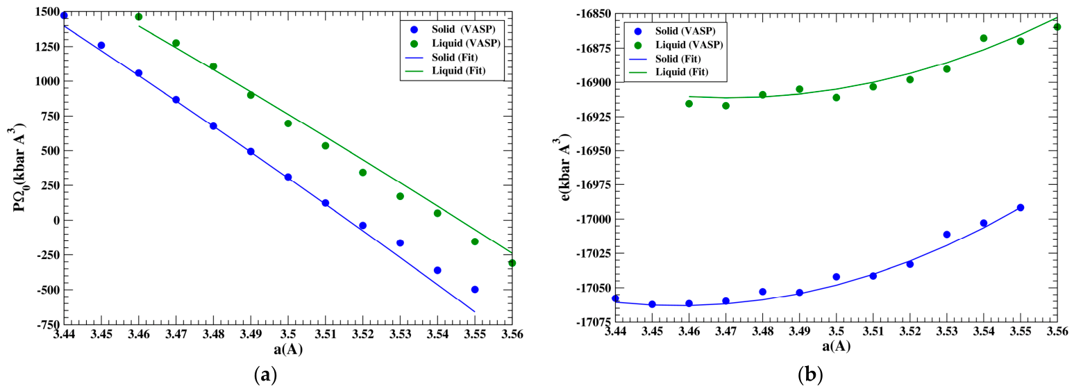
For U-6Nb, the best fits of the forms (22), (23) that describe our VASP results on both P•Ω₀ = P•Ω₀(a) and e = e(a) simultaneously are (in kbar ų):

$$P•{\Omega }_{0_s}\left(a\right) = 6788.75 a^{3/2}-1029.71 a^3,e_s\left(a\right) = 26,578.3 – 13,577.5{ a}^{3/2}+ 1056.05 a^3$$

(24)

for solid and

$$P•{\Omega }_{0_l}\left(a\right)=6003.08 a^{3/2}-899.013 a^3,e_l\left(a\right)=21,907.4 – 12,006.2{ a}^{3/2}+928.350 a^3$$

(25)

for liquid. The two values of the lattice constant a that correspond to P = 0 are

a_s = 3.516 Å and a_l = 3.546 Å.

(26)

Calculated RDFs of the solid and liquid U₁₁₁Nb₁₇ alloy at T_m = 1572 K are shown in Figure 6. The character features of the solid and liquid phases (see Appendix A) are clearly seen.

The volume change at the melting temperature is:

$${\Delta V}_m= {\left({\displaystyle \frac{a_l}{a_s}}\right)}^3-1= {\left({\displaystyle \frac{3.546}{3.516}}\right)}^3-1= 0.026,$$

(27)

i.e., 2.6%. The values of es(as) and e_l(a_l) are −17,034.2 kbar ų and −16,869.8 kbar ų, respectively. Therefore, the value of L_m is 164.4 kbar ų, or $0.103{\displaystyle \frac{eV}{atom}}$, or $9.9{\displaystyle \frac{\mathrm{k}\mathrm{J}}{\mathrm{m}\mathrm{o}\mathrm{l}}}$. According to Hackenberg [116], the latent heat of melting cannot be defined in a classical thermodynamic manner. Instead, he suggested defining it as the enthalpy difference between the extrapolated single phase solidus and liquidus lines, ΔH (T₀), where T₀ = 1290 °C (1563 K), fairly close to the calculated T_m = 1572 K of the U₁₁₁Nb₁₇ alloy, is the so-called median temperature between the solidus and liquidus lines of the U-Nb phase diagram at U-6Nb composition. According to [116], $L_m^{exp.}=12.615{\displaystyle \frac{\mathrm{k}\mathrm{J}}{\mathrm{m}\mathrm{o}\mathrm{l}}}$ and the calculated $L_M=9.9{\displaystyle \frac{\mathrm{k}\mathrm{J}}{\mathrm{m}\mathrm{o}\mathrm{l}}}$ represents ~78.5% of $L_m^{exp.}$.

Our QMD data points of P•Ω₀ = P•Ω₀ (a) and E = E(a), along with the corresponding fits, are shown in Figure 7a,b, respectively.

4.2.4. Accuracy of the Results on the Latent Heat of Fusion and Volume Change at Melt

Our results on both the latent heat of fusion and volume change at melt are accurate enough, as they appear to be virtually independent of the functional form of the fits to our QMD data, from which the values of e(a) and $P•{\mathsf{\Omega }}_0\left(a\right)$ for both solid and liquid come and which give rise to the values of L_m and ${\Delta V}_m$. In addition to (22) and (23), we used two other functional forms, and the corresponding values of L_m and ${\Delta V}_m$ appear to lie in the intervals, respectively, 9.9 ± 0.2 kJ/mol and 2.6 ± 0.1%, which may be considered as our theoretical values with the corresponding error bars. Note that these values for a 128-atom system are fully consistent with those for the 250-atom system considered in our previous work [70], namely, 9.7 kJ/mol and 2.6%, which come from the application of a similar fitting procedure described above to the results of [70]; see Section 7 for more detail.

5. Self-Diffusion and Viscosity of U-6Nb Alloy

We calculate the self-diffusion coefficient of the liquid U₁₁₁Nb₁₇ alloy using Equation (1) which requires the knowledge of MSD as a function of time, Equation (2). The knowledge of the self-diffusion coefficient allows calculation of the viscosity by the modified Stokes–Einstein relation, Equation (3).

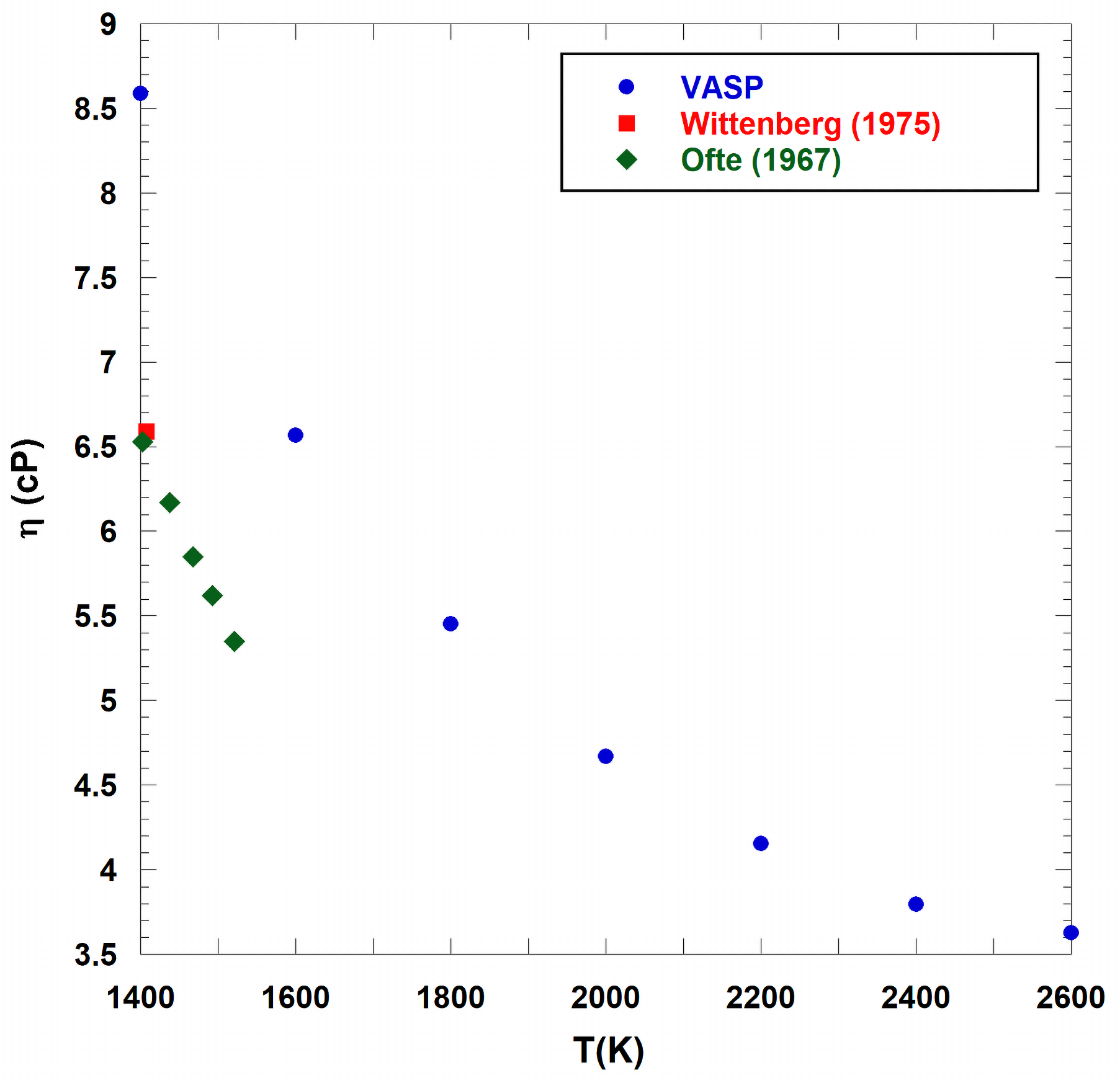
The temperature dependence of the calculated self-diffusion coefficient and viscosity of the liquid U₁₁₁Nb₁₇ alloy are shown in

Table 2. Self-diffusion coefficient, D, and viscosity, η, of the U_86.72Nb_13.28 alloy at different temperatures.

T (K)	D (10−8 m2/s)	η (cP)
1400	0.1139	8.5890
1600	0.1730	6.5672
1800	0.2394	5.4505
2000	0.3105	4.6697
2200	0.3841	4.1523
2400	0.4586	3.7940
2600	0.5328	3.6289

. Like it was in the case of the density and specific heat, there are no experimental data on the viscosity of the liquid U₁₁₁Nb₁₇ alloy. Figure 8 shows the calculated viscosity of the liquid U₁₁₁Nb₁₇ alloy together with available experimental data on the viscosity of pure liquid uranium [117,118].

6. Thermal Conductivity Calculation

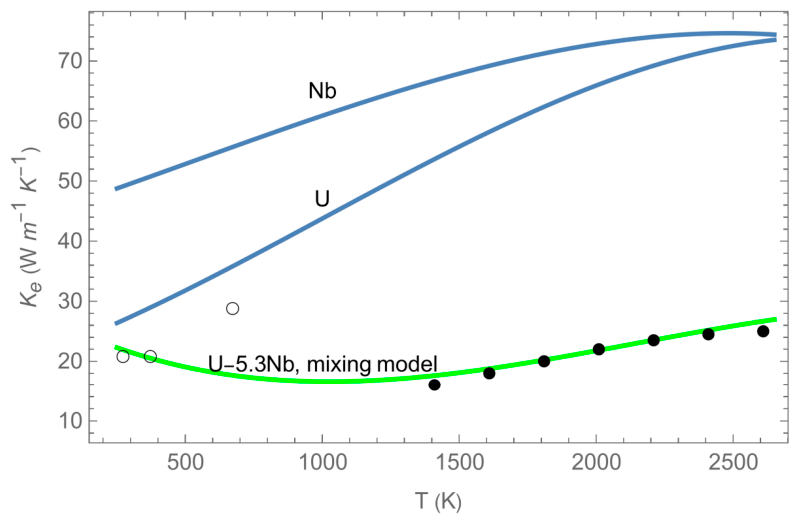
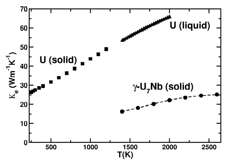
Figure 9 shows our results for the electronic contribution to thermal conductivity (κ_e). These results are for the solid γ-U₇Nb (ordered) alloy and serve here as an approximation for the corresponding liquid. The absolute atomic volume as a function of temperature for the liquid is being used in calculations and therefore the appropriate liquid thermal expansion is accounted for (Table 1). The lattice-vibration contribution (κ_lat) was estimated separately from the temperature-dependent phonons of γ-uranium and is considerably smaller than the electronic contribution (κ_lat~1 WK⁻¹m⁻¹).

The experimental data on the thermal conductivity of pure solid and liquid uranium are also shown in Figure 9. We note a significant difference between our ab initio results and those of the experimental results for unalloyed solid and liquid uranium in Figure 9. The reasons for this difference must be: (i) the addition of Nb in uranium plays a significant role, (ii) the theory assumes a perfectly ideal material with no imperfections that do exist in the real material, and (iii) the calculations furthermore assume that the phonons are harmonic, which is an approximation. It appears most of the difference can be traced to the ab initio calculated electronic relaxation time, τ. If used as a fitting parameter, one can easily reproduce the experimental behavior of elemental uranium.

However, the thermal conductivity of the U-Nb alloy appears to be below that of pure U, which seems to be confirmed by both direct experimental data on U-6Nb of Ref. [119] and theoretical calculations on the alloys U-Zr and U-Mo with similarly low content of solute elements [120]. It appears that in low concentrations alloying atoms act as impurities causing lattice distortion, which results in the reduction in the thermal conductivity of the alloy compared to that of pure solvent (U). Generally, as a function of the alloying concentration, the thermal conductivity of an alloy is expected to decrease, reach a minimum, and at higher concentrations increase towards its value for pure alloying solute (Nb).

The widely accepted Filippov’s [121] (also derived by Rowley [122,123]) model for the thermal conductivity of a binary mixture, κ_m, reads:

κ_m = w₁κ₁ + w₂κ₂ − R|κ₁ − κ₂|w₁w₂,

(28)

where κ₁ and κ₂ are the thermal conductivities of constituents 1 and 2, w₁ and w₂ are the corresponding weight fractions, and R is a positive constant (the use of the absolute value of κ₁ − κ₂ ensures that κ_m is smaller than either κ₁ or κ₂) which may be temperature-dependent. Using the analytic forms of the thermal conductivities of pure U (which interpolates smoothly between those of solid and liquid U shown in Figure 9) and pure Nb (which applies to both solid and liquid [124]):

κ(U) = 26.4 + 2.05 10⁻² (T−250) + 5.40 10⁻⁶ (T−250)² − 2.40 10⁻⁹ (T−250)³

(29)

κ(Nb) = 48.0 + 1.6 10⁻² (T−200) + 1.3 10⁻⁶ (T−200)² − 1.40 10⁻⁹ (T−200)³

(30)

it is possible to find R = R(T) such that the resulting κ_m interpolates smoothly between experiment [119] and our calculations. Note that in our calculations the ordered structure of 28 U and 4 Nb atoms is considered which corresponds to 12.5 at.%, or 5.3 wt.% Nb, which is slightly different from U-6 wt.% Nb (U-6Nb). The model curve is shown in Figure 10. The corresponding analytic form is:

κ_m = 22.3 − 1.6 10⁻² (T−250) + 1.3 10⁻⁵ (T−250)² − 2.3 10⁻⁹ (T−250)³.

(31)

This model curve Equation (31) is shown in Figure 10 as a green line, along with the thermal conductivities of pure U and Nb described by the above formulas, the experimental data on U-6Nb of Ref. [119] (empty circles), and our theoretical calculations on γ-U7Nb (filled circles).

We understand that modeling the true U-6Nb liquid with a solid supercell γ-U7Nb is an approximation. We are not able to assess the uncertainty of this simplification, but it cannot easily be avoided, as the first-principles methodology needs further development to address the nature of the liquid. Certainly, the disorder of the liquid is ignored. The perhaps larger discrepancy with pure U than expected is most likely associated with our underestimation of the calculated relaxation time, τ, as we have discussed. We are currently developing methodology to better compute this parameter from first-principles theory.

7. Discussion and Conclusions

By means of ab initio quantum molecular dynamics (VASP) we calculate the main thermophysical parameters that could be used in the modeling of U-6Nb alloys casting. As was in the case of the liquid U₁₁₆Nb₁₂ alloy [51], the density and thermal expansion coefficient of the liquid U₁₁₁Nb₁₇ alloy show a linear dependence with temperature. Conversely, the specific heat at constant pressure of the liquid U₁₁₁Nb₁₇ alloy remains constant within the specified temperature range, 1400 K ≤ T ≤ 2600 K.

We present the results of calculations of the melting temperature of the U₁₁₁Nb₁₇ alloy, T_m = 1572 K, which is based on the Z-method. The calculated latent heat of melting is equal to $\mathbf{9.9}{\displaystyle \frac{\mathit{k}\mathit{J}}{\mathit{m}\mathit{o}\mathit{l}}}$, and the calculated volume change at melting is equal to 2.6%. The use of the Clausius–Clapeyron formula for the initial slope of the melting curve, ${\left({\displaystyle \frac{\mathit{d}{\mathit{T}}_{\mathit{m}}}{\mathit{d}\mathit{p}}}\right)}_{\mathit{p}=\mathbf{0}}$ = ${\displaystyle \frac{{\mathit{T}}_{\mathit{m}}\mathit{\Delta }{\mathit{V}}_{\mathit{m}}}{{\mathit{L}}_{\mathit{m}}}}$, with the volume change at melt $\mathbf{\Delta }{\mathit{V}}_{\mathit{m}}=\mathbf{0.34}{\displaystyle \frac{{\mathbf{c}\mathbf{m}}^3}{\mathbf{m}\mathbf{o}\mathbf{l}}}$, the difference between the molar volumes of 13.43 ${\displaystyle \frac{{\mathbf{c}\mathbf{m}}^3}{\mathbf{m}\mathbf{o}\mathbf{l}}}$ of solid and 13.09 ${\displaystyle \frac{{\mathbf{c}\mathbf{m}}^3}{\mathbf{m}\mathbf{o}\mathbf{l}}}$ of liquid, along with T_m=1572 K and ${\mathit{L}}_{\mathit{M}}=\mathbf{9.9}{\displaystyle \frac{\mathbf{k}\mathbf{J}}{\mathbf{m}\mathbf{o}\mathbf{l}}}$, gives ${\left({\displaystyle \frac{\mathit{d}{\mathit{T}}_{\mathit{m}}}{\mathit{d}\mathit{p}}}\right)}_{\mathit{p}=\mathbf{0}}=\mathbf{5.40}{\displaystyle \frac{\mathbf{K}}{\mathbf{k}\mathbf{b}\mathbf{a}\mathbf{r}}}$, which is within 10% of $\mathbf{4.92}{\displaystyle \frac{\mathbf{K}}{\mathbf{k}\mathbf{b}\mathbf{a}\mathbf{r}}}$ from Ref. [70].

We carried out a similar analysis of a 250-atom model of U-6Nb as U₂₁₅Nb₃₅. (14 at.% Nb) [70]. It appears that in this case the values of both ΔV_m and L_m remain essentially the same as before. Specifically, the lattice dimensions of the solid and liquid systems at T_m = 1572 K are, respectively, 3.517 Å and 3.547 Å (in the 128-atom case they are 3.516 Å and 3.546 Å), so that the volume change at melt is again 2.6%. The latent heat of melting turns out to be $\mathbf{9.7}{\displaystyle \frac{\mathit{k}\mathit{J}}{\mathit{m}\mathit{o}\mathit{l}}}$, which is a little less than, yet fully consistent with $\mathbf{9.9}{\displaystyle \frac{\mathbf{k}\mathbf{J}}{\mathbf{m}\mathbf{o}\mathbf{l}}}$ in the 128-atom case. Hence, the results for both 128-atom and 250-atom systems are fully consistent with each other, which means that the 128-atom system used in our study is fully converged as regards the thermal EOS and the ambient melting point.

The canonical Stokes–Einstein relation, Equation (4), for a sphere in the Newtonian fluid has the factor 3π in the denominator. For liquid metals, the modified Stokes–Einstein relation, Equation (3), is often used, where the factor 2π reflects a different friction model suitable for atoms in metals. We define the self-diffusion coefficient of the liquid U₁₁₁Nb₁₇ alloy through the mean-square displacement calculations. The modified Stokes–Einstein relation is used to calculate the viscosity of U-6Nb alloy. Addition of niobium to liquid uranium decreases diffusivity and, thus, increases the viscosity.

For the first time, the thermal conductivity of U₇Nb alloys is calculated. To date, all calculations of thermal conductivity of uranium alloys have been conducted using the Boltzmann transport equations within CRTA, where the relaxation time τ is not calculated from first principles but rather fitted to the experimental resistivity measurements. The calculation of τ is quite challenging and involves comprehensive calculations of electron–phonon matrix elements. The ab initio relaxation time calculations reported here have two ramifications: (i) the temperature dependence is found to be weak, and (ii) the calculations significantly underestimate the value of τ necessary to match experimental measurements. This is most likely due to the strong anharmonic nature of the phonons in entropically stabilized γ-U, yielding the self-energy relaxation time approximation applied to a perfect γ-U lattice significantly underestimating the electron scattering rates. It is also important to note that the calculations show that in accord with most metals, τ in γ-U can be considered nearly temperature independent. This contrasts with recent works [125,126] where τ is modeled via an inverse temperature dependence: ${\displaystyle \frac{1}{\mathit{\tau }}}$ = A${\mathit{T}}^2+\mathit{B}\mathit{T}$, where A and B parameters are fitted to resistivity measurements.

References

1. Hofman, G.L.; Walters, L.C.; Bauer, T.H. Metallic Fast reactors fuels. Prog. Nucl. Energy 1997, 31, 83–110. [Google Scholar] [CrossRef]
2. Keiser, D.D., Jr.; Kennedy, J.B.; Hilton, B.A.; Hayes, S.L. The development of metallic nuclear fuels for transmutation applications: Materials challenges. JOM 2008, 60, 29–32. [Google Scholar] [CrossRef]
3. Carmack, W.J.; Porter, D.L.; Chang, Y.I.; Hayes, S.L.; Meyer, M.K.; Burkes, D.E.; Lee, C.B.; Mizuno, T.; Delage, F.; Somers, J. Metallic fuels for advanced reactors. J. Nucl. Mater. 2009, 392, 139–150. [Google Scholar] [CrossRef]
4. Tangri, K.; Williams, G. Metastable phases in the uranium molybdenum system and their origin. J. Nucl. Mater. 1961, 4, 226–233. [Google Scholar] [CrossRef]
5. Howlett, B.A. Study of the shear transformations from the gamma-phase in uranium-molybdenum alloys containing 6.0–12.5 at % molybdenum. J. Nucl. Mater. 1970, 35, 278–292. [Google Scholar] [CrossRef]
6. Anagnostidis, M.; Colombie, M.; Monti, H. Phases metastables dans les alliages uranium-niobium. J. Nucl. Mater. 1964, 11, 67–76. [Google Scholar] [CrossRef]
7. Tangri, K.; Chaudhuri, D.K. Metastable phases in uranium alloys with high solute solubility in the BCC gamma phase. Part I—The System U-Nb. J. Nucl. Mater. 1965, 15, 278–287. [Google Scholar] [CrossRef]
8. Takahashi, Y.; Yamawaki, M.; Yamamoto, K. Thermophysical properties of uranium-zirconium alloys. J. Nucl. Mater. 1988, 154, 141–144. [Google Scholar] [CrossRef]
9. Ma, J.J.; Han, X.F.; Cai, X.X.; Qiu, R.Z.; Eriksson, O.; Zhang, P.; Wang, B.-T. High- temperature mechanical and dynamical properties of γ-(U,Zr) alloys. Materials 2023, 16, 2623. [Google Scholar] [CrossRef]
10. Kahana, E.; Talianker, M.; Landau, A. Formation of the monoclinic α” phase in quenched U-3.6 at.% Ti-4.7 at.% W alloy. J. Nucl. Mater. 1997, 246, 144–149. [Google Scholar] [CrossRef]
11. Speer, J.; Edmonds, D. An investigation of the γ → α martensitic transformation in uranium alloys. Acta Metall. 1988, 36, 1015–1033. [Google Scholar] [CrossRef]
12. Donohue, J. The Structures of the Elements; John Wiley & Sons: New York, NY, USA, 1974. [Google Scholar] [CrossRef]
13. Arblaster, J.W. Selected Values of the Crystallographic Properties of the Elements; ASM International: Materials Park, OH, USA, 2018. [Google Scholar]
14. Söderlind, P.; Grabowski, B.; Yang, L.; Landa, A.; Björkman, T.; Souvatzis, P.; Eriksson, O. High-temperature phonon stabilization of γ-uranium from relativistic first-principles theory. Phys. Rev. B 2012, 85, 060301. [Google Scholar] [CrossRef]
15. Eckelmeyer, K.H.; Romig, A.D.; Weirick, L.J. The effect of quench rate on the microstructure, mechanical properties, and corrosion behavior of U-6 wt pct Nb. Metall. Trans. A 1984, 15, 1319–1330. [Google Scholar] [CrossRef]
16. Vandermeer, R. Phase transformations in a uranium + 14 at.% niobium alloy. Acta Metall. 1980, 28, 383–393. [Google Scholar] [CrossRef]
17. Vandermeer, R.A.; Ogle, J.C.; Northcutt, W.G. A phenomenological study of the shape memory effect in polycrystalline uranium-niobium alloys. Metall. Trans. A 1981, 12, 733–741. [Google Scholar] [CrossRef]
18. Lillard, J.A.; Hanrahan, R.J., Jr. Corrosion of uranium and uranium alloys. In Corrosion: Materials; Cramer, S.D., Covino, B.S., Eds.; ASM International: Materials Park, OH, USA, 2005; Volume 13B, pp. 370–384. [Google Scholar]
19. Koike, J.; Kassner, M.E.; Tate, R.E.; Rosen, R.S. The Nb-U (Niobium-Uranium) system. J. Phase Equilib. 1998, 19, 253–260. [Google Scholar] [CrossRef]
20. Field, R.D.; Thoma, D.J.; Dunn, P.S.; Brown, D.W.; Cady, C.M. Martensitic structures and deformation twinning in the U-Nb shape-memory alloys. Philos. Mag. A 2001, 81, 1691–1724. [Google Scholar] [CrossRef]
21. Hackenberg, R.E.; Brown, D.W.; Clarke, A.J.; Dauelsberg, L.B.; Field, R.D.; Hults, W.L.; Kelly, A.M.; Lopez, M.F.; Teter, D.F.; Thoma, D.J.; et al. U–Nb Aging Final Report; Los Alamos National Laboratory Preprint, Report No. LA-14327; Los Alamos National Laboratory: Los Alamos, NM, USA, 2007.
22. Liu, X.J.; Li, Z.S.; Wang, J.; Wang, C.P. Thermodynamic modeling of the U–Mn and U–Nb systems. J. Nucl. Mater. 2008, 380, 99–104. [Google Scholar] [CrossRef]
23. Duong, T.C.; Hackenberg, R.E.; Landa, A.; Honarmandi, P.; Talapatra, A.; Volz, H.M.; Llobet, A.; Smith, A.I.; King, G.; Bajaj, S.; et al. Revisiting thermodynamics and kinetic diffusivities of uranium–niobium with Bayesian uncertainty analysis. Calphad 2016, 55, 219–230. [Google Scholar] [CrossRef]
24. Duong, T.C.; Hackenberg, R.E.; Attari, V.; Landa, A.; Turchi, P.E.; Arróyave, R. Investigation of the discontinuous precipitation of U-Nb alloys via thermodynamic analysis and phase-field modeling. Comput. Mater. Sci. 2020, 175, 109573. [Google Scholar] [CrossRef]
25. Volz, H.; Hackenberg, R.; Kelly, A.; Hults, W.; Lawson, A.; Field, R.; Teter, D.; Thoma, D. X-ray diffraction analyses of aged U–Nb alloys. J. Alloys Compd. 2007, 444–445, 217–225. [Google Scholar] [CrossRef]
26. Clarke, A.; Field, R.; Hackenberg, R.; Thoma, D.; Brown, D.; Teter, D.; Miller, M.; Russell, K.; Edmonds, D.; Beverini, G. Low temperature age hardening in U–13 at.% Nb: An assessment of chemical redistribution mechanisms. J. Nucl. Mater. 2009, 393, 282–291. [Google Scholar] [CrossRef]
27. Hackenberg, R.; Volz, H.M.; Papin, P.A.; Kelly, A.M.; Forsyth, R.T.; Tucker, T.J.; Clarke, K. Kinetics of lamellar decomposition reactions in U-Nb alloys. Solid State Phenom. 2011, 172–174, 555–560. [Google Scholar] [CrossRef]
28. Djurič, B. Decomposition of gamma phase in a uranium-9.5 wt % niobium alloy. J. Nucl. Mater. 1972, 44, 207–214. [Google Scholar] [CrossRef]
29. Cahn, J. The kinetics of cellular segregation reactions. Acta Metall. 1959, 7, 18–28. [Google Scholar] [CrossRef]
30. Zhang, J.; Brown, D.W.; Clausen, B.; Vogel, S.C.; Hackenberg, R.E. In situ time-resolved phase evolution and phase transformations in U-6 wt pct Nb. Metall. Mater. Trans. A 2019, 50, 2619–2628. [Google Scholar] [CrossRef]
31. Brown, D.W.; Bourke, M.A.M.; Dunn, P.S.; Field, R.D.; Thoma, M.J. Uniaxial tensile deformation of uranium 6 wt pct niobium: A neutron diffraction study of deformation twinning. Metall. Trans. A 2001, 32, 2219–2228. [Google Scholar] [CrossRef]
32. Brown, D.W.; Bourke, M.A.M.; Field, R.D.; Hults, W.L.; Teter, D.F.; Thoma, D.J.; Vogel, S.C. Neutron diffraction study of the deformation mechanism of the uranium-7 wt.% niobium shape memory alloy. Mater. Sci. Eng. A 2006, 421, 15–21. [Google Scholar] [CrossRef]
33. Tupper, C.N.; Brown, D.W.; Field, R.D.; Sisneros, T.A.; Clausen, B. Large strain deformation in uranium 6 wt pct niobium. Metall. Mater. Trans. A 2012, 43, 520–530. [Google Scholar] [CrossRef]
34. Brown, D.W.; Bourke, M.A.M.; Clarke, A.J.; Field, R.D.; Hackenberg, R.D.; Hults, W.L.; Thoma, D.J. The effect of low-temperature aging on the microstructure and deformation of uranium 6 wt% niobium: An in-situ neutron diffraction study. J. Nucl. Matter. 2016, 481, 164–175. [Google Scholar] [CrossRef]
35. Wu, A.S.; Brown, D.W.; Clausen, B.; Elmer, J.W. The influence of impurities on the crystal structure and mechanical properties of additive manufactured U-14 at. % Nb. Scr. Mater. 2017, 130, 59–63. [Google Scholar] [CrossRef]
36. Zhang, J.; Vogel, S.C.; Brown, D.; Clausen, B.; Hackenberg, R. Equation of state, phase stability, and phase transformations of uranium-6 wt.% niobium under high pressure and temperatures. J. Appl. Phys. 2018, 123, 175103. [Google Scholar] [CrossRef]
37. Rosen, R.S.; Kassner, M.E.; Thiehsen, K.E. The mechanical behaviour of U-6Nb alloy and AISI 1045 and 1215 steels at high strain rates. J. Mater. Sci. Lett. 1992, 11, 125–128. [Google Scholar] [CrossRef]
38. Zhang, C.; Wang, H.; Li, J.; Pang, B.B.; Xia, Y.; Liu, Y.; Sun, G.; Zhang, X.; Fa, T.; Wang, X. The aging-effect-modulated mechanical behavior in U-Nb shape memory alloys through the modified twinning-detwinning process of the α’’ phase. Mater. Des. 2019, 162, 94–105. [Google Scholar] [CrossRef]
39. Eckelmeyer, K.H. Residual stresses and stress relieving in uranium alloys. In Residual Stress and Stress Relaxation. Sagamore Army Materials Research Conference Proceedings; Kula, E., Weiss, V., Eds.; Springer: Boston, MA, USA, 1982; Volume 28, pp. 389–407. [Google Scholar] [CrossRef]
40. Zhang, J.; Hackenberg, R.; Vogel, S.C.; Brown, D. Equation of state and phase evolution of U-7.7Nb with implications for the understanding of dynamic behaviour of U-Nb alloys. Appl. Phys. Lett. 2019, 114, 221901. [Google Scholar] [CrossRef]
41. Govindjee, S.; Kasper, E.P. A shape memory alloy model for uranium-niobium accounting for plasticity. J. Intell. Mater. Syst. Struct. 1997, 8, 815–823. [Google Scholar] [CrossRef]
42. Addessio, F.L.; Zuo, Q.H.; Mason, T.A. Model for high-strain-rate deformation of uranium-niobium alloys. J. Appl. Phys. 2003, 93, 9644–9654. [Google Scholar] [CrossRef]
43. Zubelewicz, A.; Addessio, F.L.; Cady, C.M. A constitutive model for uranium-niobium alloy. J. Appl. Phys. 2006, 100, 013523. [Google Scholar] [CrossRef]
44. Zhang, J.; Hackenberg, R.E.; Watkins, E.B.; Vogel, S.C.; Brown, D.W. The lattice parameter –composition relationship of the body centered cubic uranium-niobium alloys. J. Nucl. Mater. 2020, 542, 152493. [Google Scholar] [CrossRef]
45. Mo, C.; Mo, W.; Zhou, P.; Bian, B.; Du, Y.; Fa, T.; Zhang, P.; Li, R.; Zhang, Y.; Zhang, C.; et al. Experimental investigation and thermodynamic modeling of the U–Nb system. J. Mater. Sci. Technol. 2021, 81, 229–235. [Google Scholar] [CrossRef]
46. Liu, F.; Zhao, Y.; Chen, L.; Yuan, L.; Shi, T.; Cui, S.; Zou, D.; He, L.; Xiao, D.; Luo, Z.; et al. A phenomenological study on the microstructure dependence of the internal friction in U-Nb shape memory alloy. Mater. Sci. Eng. A 2023, 883, 145470. [Google Scholar] [CrossRef]
47. Xiang, X.; Huang, H.; Hsiung, L.M. Quantum mechanical calculations of uranium phases and niobium defects in γ-uranium. J. Nucl. Mater. 2008, 375, 113–119. [Google Scholar] [CrossRef]
48. Lu, C.; Ni, S.; Chen, W.; Zhang, C.; Wang, Y. Influence of electron energy loss spectroscopy of the niobium-substituted uranium atom: A density functional theory study. Nucl. Sci. Techn. 2008, 19, 365–369. [Google Scholar]
49. Dai, Y.; Lu, C.H.; Ren, Q.B.; Lu, L.; Li, J.H.; Liu, B.X. A long-range U–Nb potential for the calculation of some chemical and physical properties of the U–Nb system. J. Nucl. Mater. 2012, 427, 239–244. [Google Scholar] [CrossRef]
50. Wang, J.-T.; Yu, W.-L.; Wang, T.; Wang, Y.-L.; Gao, Y.-L. First-principles study on thermodynamic defect and crystal structure of U-12.5 at.% Nb alloy. Int. J. Heat Technol. 2015, 33, 175–180. [Google Scholar] [CrossRef]
51. Shi, Y.; Liu, M.; Chen, Y.; Wang, X.; Mo, W.; Li, D.; Fa, T.; Bai, B.; Wang, X.; Chen, X.-Q. Evolution of local atomic structure during solidification of U116Nb12 liquid: An ab initio molecular dynamics study. J. Alloys Compd. 2019, 787, 267–275. [Google Scholar] [CrossRef]
52. Landa, A.; Söderlind, P.; Wu, A. Phase stability in U-6Nb alloy doped with Ti from the first principles theory. Appl. Sci. 2020, 10, 3417. [Google Scholar] [CrossRef]
53. Söderlind, P.; Yang, L.H.; Landa, A.; Wu, A. Mechanical and thermal properties for uranium and U–6Nb alloy from first-principles theory. Appl. Sci. 2021, 11, 5643. [Google Scholar] [CrossRef]
54. Pan, X.L.; Wang, H.; Zhang, L.L.; Wang, Y.F.; Chen, X.R.; Geng, H.Y. Prediction of novel final phases in aged uranium-niobium. J. Nucl. Mater. 2023, 579, 154394. [Google Scholar] [CrossRef]
55. Bao, N.; Tong, Q.; Guo, F.; Zhang, S.; Kang, D.; Akinpelu, A.; Lv, J.; Yao, Y.; Dai, J. Structures and properties of uranium–niobium intermetallic compounds under high pressure: A first principles study. J. Appl. Phys. 2023, 133, 095901. [Google Scholar] [CrossRef]
56. Wen, X.; Li, C.; Liu, T. Ab initio molecular dynamics study of Nb doping on temperature-driven structural stability and diffusion kinetics of U-6Nb alloys. J. Alloy. Compd. 2025, 1042, 184077. [Google Scholar] [CrossRef]
57. Wen, X.; Li, C.Y.; Liu, T. Effects of Nb doping and crystal symmetry on the structural stability and mechanical properties at U-Nb twin boundaries. J. Alloys Compd. 2025, 1025, 180200. [Google Scholar] [CrossRef]
58. Huang, Y.; Yao, S.; Chen, H.; Li, P.; Wang, K.; Chen, J.; Deng, H.; Hu, W. An atomistic study of γ → γ0 → α’’ martensitic transformation in uranium-6wt % niobium. J. Nucl. Mater. 2025, 606, 155617. [Google Scholar] [CrossRef]
59. Ludwig, A. Thermophysical Properties Necessary for Advanced Casting Simulations. Int. J. Thermophys. 2002, 23, 1131–1146. [Google Scholar] [CrossRef]
60. Venkatesana, A.; Gobinath, V.M.; Rajadurai, A. Simulation of casting solidification and its grain structure prediction using FEM. J. Mater. Process. Technol. 2005, 168, 10–15. [Google Scholar] [CrossRef]
61. Kermanpur, A.; Mahmoudi, S.h.; Hajipour, A. Numerical simulation of metal flow and solidification in the multi-cavity casting molds of automotive components. J. Mater. Process. Techol. 2008, 206, 62–68. [Google Scholar] [CrossRef]
62. Hofer, P.; Kaschnitz, E.; Schumacher, P. Simulation of distortion and residual stress in high pressure die casting—Modelling and experiments. IOP Conf. Ser. Mater. Sci. Eng. 2002, 33, 012055. Available online: http://iopscience.iop.org/1757-899X/33/1/012055 (accessed on 29 March 2026). [CrossRef]
63. Blöchl, P.E. Projector augmented-wave method. Phys. Rev. B 1994, 50, 17953–17978. [Google Scholar] [CrossRef]
64. Kresse, G.; Hafner, J. Ab initio molecular dynamics for liquid metals. Phys. Rev. B 1993, 47, 558–561. [Google Scholar] [CrossRef] [PubMed]
65. Kresse, G.; Furthmüller, J. Efficiency of ab-initio total energy calculations for metals and semiconductors using a plane-wave basis set. Comput. Mater. Sci. 1996, 6, 15–50. [Google Scholar] [CrossRef]
66. Kresse, G.; Furthmüller, J. Efficient iterative schemes for ab initio total-energy calculations using a plane-wave basis set. Phys. Rev. B 1996, 54, 11169–11186. [Google Scholar] [CrossRef]
67. Kresse, G.; Joubert, D. From ultrasoft pseudopotentials to the projector augmented-wave method. Phys. Rev. B 1999, 59, 1758–1775. [Google Scholar] [CrossRef]
68. Perdew, J.P.; Burke, K.; Ernzerhof, M. Generalized gradient approximation Made Simple. Phys. Rev. Lett. 1996, 77, 3865–3868. [Google Scholar] [CrossRef]
69. Mermin, K.D. Thermal properties of the inhomogeneous electron gas. Phys. Rev. 1965, 137, A1441–A1443. [Google Scholar] [CrossRef]
70. Burakovsky, L.; Preston, D.L.; Green, A.A. Analytic Model for U-Nb Liquidus and U-6Nb Melting Curve. Appl. Sci. 2025, 15, 3763. [Google Scholar] [CrossRef]
71. Nosé, S. Molecular dynamics method for simulations in the canonical ensemble. Mol. Phys. 1994, 52, 255–268. [Google Scholar] [CrossRef]
72. Hoover, W.G. Canonical dynamics: Equilibrium phase-space distributions. Phys. Rev. A 1985, 31, 1695–1697. [Google Scholar] [CrossRef]
73. Verlet, L. Computer “Experiments” on classical fluids. I. Thermodynamical properties of Lennard-Jones Molecules. Phys. Rev. 1967, 59, 98–103. [Google Scholar] [CrossRef]
74. Verlet, L. Computer “Experiments” on Classical Fluids. II. II. Equilibrium correlation functions. Phys. Rev. 1968, 165, 201–214. [Google Scholar] [CrossRef]
75. Swope, W.C.; Andersen, H.C.; Berens, P.H.; Wilson, K.R. A computer simulation method for the calculation of equilibrium constants for the formation of physical clusters of molecules: Application to small water clusters. J. Chem. Phys. 1982, 76, 637–649. [Google Scholar] [CrossRef]
76. Zheng, H.; Wang, S.; Zhang, Y. Increasing the time step with mass scaling in Born-Oppenheimer ab initio QM/MM molecular dynamics simulations. J. Comput. Chem. 2009, 30, 2706–2711. [Google Scholar] [CrossRef]
77. Belonoshko, A.B.; Skorodumova, N.V.; Rosengren, A.; Johansson, B. Melting and critical superheating. Phys. Rev. B 2006, 73, 012201. [Google Scholar] [CrossRef]
78. Belonoshko, A.B.; Davis, S.; Skorodumova, N.V.; Lundow, P.H.; Rosengren, A.; Johansson, B. Properties of the fcc Lennard-Jones crystal model at the limit of superheating. Phys. Rev. B 2007, 76, 064121. [Google Scholar] [CrossRef]
79. Cricchio, F.; Belonoshko, A.B.; Burakovsky, L.; Preston, D.L.; Ahuja, R. High-pressure melting of lead. Phys. Rev. B 2006, 73, 140103(R). [Google Scholar] [CrossRef]
80. Belonoshko, A.B.; Burakovsky, L.; Chen, P.; Johansson, B.; Mikhaylushkin, A.S.; Preston, D.L.; Simak, S.I.; Swift, D.C. Molybdenum at High Pressure and Temperature: Melting from another solid phase. Phys. Rev. Lett. 2008, 100, 1357014. [Google Scholar] [CrossRef]
81. Belonoshko, A.B.; Rosengren, A.; Burakovsky, L.; Preston, D.L.; Johansson, B. Melting of Fe and Fe0.9375Si0.0625 at Earth’s core pressures studied using ab initio molecular dynamics. Phys. Rev. B 2009, 79, 220102(R). [Google Scholar] [CrossRef]
82. Belonoshko, A.B.; Arapan, S.; Martonak, R.; Rosengren, A. MgO phase diagram from first principles in a wide pressure-temperature range. Phys. Rev. B 2010, 81, 054110. [Google Scholar] [CrossRef]
83. Burakovsky, L.; Chen, S.P.; Preston, D.L.; Belonoshko, A.B.; Rosengren, A.; Mikhaylushkin, A.S. High-pressure—High-temperature polymorphism in Ta: Resolving an ongoing experimental controversy. Phys. Rev. Lett. 2010, 104, 255702. [Google Scholar] [CrossRef]
84. Burakovsky, L.; Chen, S.; Preston, D.L.; Sheppard, D.G. Z methodology for phase diagram studies platinum and tantalum as examples. J. Phys. Confer. Ser. 2014, 500, 162001. [Google Scholar] [CrossRef]
85. Belonoshko, A.B.; Rosengren, A. High-pressure melting curve of platinum from ab initio Z method. Phys. Rev. B 2012, 85, 174104. [Google Scholar] [CrossRef]
86. Burakovsky, L.; Preston, D.L.; Errandonea, D. Ab initio study of randomly disordered hexagonal close-packed (rhcp) phase in platinum. J. Appl. Phys. 2025, 137, 015109. [Google Scholar] [CrossRef]
87. Davis, S.; Belonoshko, A.B.; Rosengren, A.; van Duin, A.C.T.; Johansson, B. Molecular dynamics simulation of zirconia melting. Cent. Eur. J. Phys. 2010, 8, 789–797. [Google Scholar] [CrossRef]
88. Burakovsky, L.; Burakovsky, N.; Preston, D.L. Ab initio melting curve of osmium. Phys. Rev. B 2015, 92, 174105. [Google Scholar] [CrossRef]
89. Errandonea, D.; MacLeod, S.G.; Ruiz-Fuertes, J.; Burakovsky, L.; McMahon, M.I.; Wilson, C.W.; Ibañez, J.; Daisenberger, D.; Popescu, C. High-pressure/high-temperature phase diagram of zinc. J. Phys. Condens. Matter 2018, 30, 295402. [Google Scholar] [CrossRef]
90. González-Cataldo, F.; Corvacho, F.; Gutiérrez, G. Melting curve of Si by means of the Z-method. IOP Conf. Ser. J. Phys. Conf. Ser. 2018, 1043, 012038. [Google Scholar] [CrossRef]
91. Braithwaite, J.; Stixrude, L. Melting of CaSiO3 perovskite at high pressure. Geophys. Res. Lett. 2019, 46, 2037–2044. [Google Scholar] [CrossRef]
92. Nguyen-Cong, K.; Williams, A.S.; Willman, J.T.; Belonoshko, A.B.; Oleynik, L.L. First principles molecular dynamics simulations of High-pressure melting of diamond. AIP Conf. Proc. 2020, 2272, 070010. [Google Scholar] [CrossRef]
93. Rehn, D.A.; Greeff, C.W.; Burakovsky, L.; Sheppard, D.G.; Crockett, S.D. Multiphase tin equation of state using density functional theory. Phys. Rev. B 2021, 103, 184102. [Google Scholar] [CrossRef]
94. Baty, S.R.; Burakovsky, L.; Errandonea, D. Ab initio phase diagram of silver. J. Phys. Condens. Matter 2021, 33, 485901. [Google Scholar] [CrossRef]
95. Baty, S.R.; Burakovsky, L.; Errandonea, D. Ab Initio phase diagram of copper. Crystals 2021, 11, 537. [Google Scholar] [CrossRef]
96. Anzellini, S.; Boccato, S.; Baty, S.R.; Burakovsky, L.; Antonangeli, D.; Errandonea, D.; Torchio, R. Melting line and thermal equation of state of fcc-cobalt: A combined experimental and computational approach. Results Phys. 2024, 56, 107218. [Google Scholar] [CrossRef]
97. Geng, M.; Mohn, C.E. Ab initio constraints on the melting of silica at high pressures up to 500 GPa. Phys. Rev. B 2024, 109, 024106. [Google Scholar] [CrossRef]
98. Allen, M.P.; Tildesley, D.J. Computer Simulation of Liquids, 2nd ed.; Oxford University Press: New York, NY, USA, 2017. [Google Scholar]
99. Einstein, A. Über die von der molekularkinetischen Theorie der Wärme geforderte Bewegung von in ruhenden Flüssigkeiten suspendierten Teilchen. Ann. Phys. 1905, 322, 549−560. [Google Scholar] [CrossRef]
100. Demmel1, F.; Tani, A. Stokes-Einstein relation of the liquid metal rubidium and its relationship to changes in the microscopic dynamics with increasing temperature. Phys. Rev. E 2009, 97, 062124. [Google Scholar] [CrossRef]
101. Hansen, J.P.; McDonald, I.R. Theory of Simple Liquids, 4th ed.; Academic Press: Oxford, UK, 2013. [Google Scholar]
102. Tritt, T.M. Thermal Conductivity: Theory, Properties< and Applications; Kluwer Academic/Plenum: New York, NY, USA, 2004. [Google Scholar]
103. Madsen, G.K.H.; Carrete, J.; Verstraete, M.J. BoltzTraP2, a program for interpolating band structures and calculating semi-classical transport coefficients. Comput. Phys. Commun. 2018, 231, 140–145. [Google Scholar] [CrossRef]
104. Söderlind, P.; Landa, A.; Moore, E.E.; Perron, P.; Roehling, J.; McKeown, J.T. High-temperature thermodynamics of uranium from ab initio modeling. Appl. Sci. 2023, 13, 2123. [Google Scholar] [CrossRef]
105. Bergman, T.L.; Lavine, A.S. Fundamentals of Heat and Mass Transfer, 8th ed.; John Wiley & Sons: Hoboken, NJ, USA, 2017. [Google Scholar]
106. Shapiro, A.B.; Summers, L.T.; Eckel, D.J.; Sahai, V. Modeling of Casting Microstructures and Defects; UCRL-ID-128519; LLNL Internal Report: Livermore, CA, USA, 1997.
107. Fokin, L.R. Liquid uranium, density isobar, 1406-3500K. Analysis and generalization of the experimental data. In Problems of Atomic Science and Technology. Serie: Nuclear-Reactor Constants; Joint Stock Company: London, UK, 2016; Issue 3; pp. 24–36. Available online: https://vant.ippe.ru/en/year2016/3/thermal-physics-hydrodynamics/1188-2.html (accessed on 4 March 2026).
108. Levinson, L.S. Heat content of molten uranium. J. Chem. Phys. 1964, 40, 3584–3585. [Google Scholar] [CrossRef]
109. Mulford, R.N.R.; Sheldon, R.I. Densi1y and heat capacity of liquid uranium at high temperatures. J. Nucl. Mater. 1988, 154, 268–275. [Google Scholar] [CrossRef]
110. Stephens, H. Determination of the enthalpy of liquid copper and uranium with a liquid argon calorimeter. High Temp. Sci. 1974, 6, 156–166. [Google Scholar]
111. Su, R.; Li, Q.; Guan, P. Construction of neural network potential for uranium-niobium alloy and molecular dynamics of its low-temperature aging behaviors. Acta Phys. Sin. 2025, 74, 056102. [Google Scholar] [CrossRef]
112. Karavaev, A.V.; Dremov, V.V.; Pravishkina, T.A. Precise calculation of melting curves by molecular dynamics. Comput. Mater. Sci. 2016, 124, 335–343. [Google Scholar] [CrossRef]
113. Rogers, B.A.; Atkins, D.F.; Manthos, E.J.; Kirkpatrick, M.E. Uranium-columbium alloy diagram. Trans. Metall. Soc. AIME 1958, 212, 387–393. [Google Scholar]
114. Drotning, W.D. Density and thermal expansion of liquid U-Nb alloy. High. Temp. High Press. 1982, 14, 253–258. [Google Scholar]
115. Burakovsky, L.; Preston, D.L.; Green, A.A. Liquidus curve of uranium-plutonium mixed oxide (MOX) system. Front. Nucl. Eng. 2025, 3, 1487828. [Google Scholar] [CrossRef]
116. Hackenberg, R.E. Liquid and Gamma-BCC Phase Equilibria in the Uranium-Niobium System: A Simple Thermodynamic Model for Phase Diagram and Other Predictions; Los Alamos Preprint LA-UR-22-27603; issued 2022-07-28; Los Alamos National Laboratory: Los Alamos, NM, USA, 2022.
117. Wittenberg, L.J. A Model for Liquid Uranium and Plutonium with Implications on the Adjacent Solid Phases. In Plutonium 1975 and Other Actinides. Proceedings of the 5th International Conference on Plutonium and Other Actinides; Blank, H., Linder, R., Eds.; North-Holland: Baden-Baden, Germany, 1976; p. 71. [Google Scholar]
118. Ofte, D. The viscosity of liquid uranium, gold and lead. J. Nucl. Mater. 1967, 22, 28–32. [Google Scholar] [CrossRef]
119. Jackson, R.J. Uranium-6Niobium. In Rocky Flats Materials Data Sheets; Report NO. RFP-1613; The Dow Chemical Company, Rocky Flats Division: Golden, CO, USA, 1971. [Google Scholar]
120. Zhou, S.; Jacobs, R.; Xie, W.; Tea, E.; Hin, C.; Morgan, D. Combined ab initio and empirical model of the thermal conductivity of uranium, uranium-zirconium, and uranium-molybdenum. Phys. Rev. Mater. 2018, 2, 083401. [Google Scholar] [CrossRef]
121. Filippov, L.P. Liquid thermal conductivity research at Moscow University. Int. J. Heat Mass Transf. 1965, 11, 331–345. [Google Scholar] [CrossRef]
122. Rowley, R.L. A local composition model for multicomponent liquid mixture thermal conductivities. Chem. Eng. Sci. 1982, 37, 897–904. [Google Scholar] [CrossRef]
123. Rowley, R.L.; White, G.L.; Chiu, M. Ternary liquid mixture thermal conductivities. Chem. Eng. Sci. 1988, 43, 361–371. [Google Scholar] [CrossRef]
124. Singaravelu, S.; Klopf, J.M.; Krafft, G.; Kelley, M.J. Laser nitriding of niobium for application to superconducting radio-frequency accelerator cavities. J. Vac. Sci. Technol. B 2011, 29, 061803. [Google Scholar] [CrossRef]
125. Zhou, S.; Zhang, Y.; Jiang, C.; Morgan, D. A combined ab-initio and empirical model for thermal conductivity of concentrated metal alloys with the focus on binary uranium alloys. Materialia 2021, 15, 100990. [Google Scholar] [CrossRef]
126. Yorgason, W.T.; Jokisaari, A.M.; Muhich, C.L. The electron thermal conductivity of Pu and Zr substituted γ-U. Nucl. Sci. Eng. 2025, 1–22. [Google Scholar] [CrossRef]
127. Hansen, J.-P.; Verlet, L. Phase transitions of the Lennard-Jones system. Phys. Rev. 1969, 184, 151–161. [Google Scholar] [CrossRef]
128. Belashchenko, D.K. Topological form restrictions on pair correlation functions of orderless systems. Russ. Metall. 1989, 3, 136–142. [Google Scholar]
129. Belashchenko, D.K. Computer simulation of liquid Pu and calculation of its physical properties at 500–5000 K. Appl. Sci. 2025, 15, 8842. [Google Scholar] [CrossRef]
130. Ott, T.; Bonitz, M.; Stanton, L.G.; Murillo, M.S. Coupling strength in Coulomb and Yukawa one-component plasmas. Phys. Plasmas 2014, 21, 113704. [Google Scholar] [CrossRef]
131. Burakovsky, L.; Preston, D.L.; Silbar, R.R. Melting as a dislocation-mediated phase transition. Phys. Rev. B 2000, 61, 15011–15018. [Google Scholar] [CrossRef]
Figure 1. The radial distribution function of the U111Nb17 alloy at 2600 K, 2200 K, 1800 K, and 1400 K.
Applsci 16 05189 g001
Figure 2. The potential energy of the U111Nb17 alloy as a function of temperature.
Applsci 16 05189 g002
Figure 3. (a) The melting pressures and temperatures calculated of the U111Nb17 alloy at different initial temperatures, Tstart. NVE computations; (b) the relation between melting pressure and temperature along the isochore, Ω0 = 21.984 Å3.
Applsci 16 05189 g003
Figure 4. (a) Time evolution of temperature during NVE QMD runs with two different initial temperatures, Tstart. During the melting run with Tstart = 3000 K, temperature decreases from ~1800 K for the superheated state to ~1558 K for a liquid at the corresponding melting point at Ω0 = 21.984 Å3. (b) Time evolution of pressure during NVE QMD run with two different initial temperatures, Tstart. During the melting run with at Tstart = 3000 K, pressure increases from ~−10 kbar for the superheated state to ~−0.61 kbar for a liquid at the corresponding melting point at Ω0 = 21.984 Å3.
Applsci 16 05189 g004
Figure 5. Radial distribution function of the U111Nb17 alloy calculated at the end of NVE QMD runs at the initial temperatures (a) Tstart = 2500 K and (b) Tstart = 3000 K.
Applsci 16 05189 g005
Figure 6. Radial distribution function of the solid (a) and liquid (b) U111Nb17 alloys calculated at the melting temperature Tm = 1572 K.
Applsci 16 05189 g006
Figure 7. (a) Pressure times atomic volume as a function of lattice constant for the solid and liquid U111Nb17 alloys: QMD data points along with the corresponding fit of the form (23); (b) total energy per atom as a function of lattice constant for the solid and liquid U111Nb17 alloys: QMD data points along with the corresponding fit of the form (22).
Applsci 16 05189 g007
Figure 8. Viscosity of the liquid U111Nb17 alloy as a function of temperature. The experimental data on the viscosity of liquid uranium [117,118] are also presented.
Applsci 16 05189 g008
Figure 9. Electronic contribution to thermal conductivity for γ-U7Nb ordered alloy. The experimental data for solid and liquid uranium are taken from [106].
Applsci 16 05189 g009
Figure 10. Thermal conductivities of pure U and Nb (blue lines) and U-5.3Nb (green line), along with the experimental data on U-6Nb of Ref. [119] (empty circles) and our theoretical calculations on γ-U7Nb (filled circles).
Applsci 16 05189 g010