Agroclimatic Forecasting Under Degraded Sensor Data: A Robustness Benchmark of Machine-Learning Models

Abstract

Reliable short-term agroclimatic forecasting is essential for precision agriculture, irrigation planning, disease-risk assessment, and microclimatic decision support. However, field-deployed sensor systems often operate under degraded data conditions, including missing measurements, noise, temporal interruptions, and limited local computational resources. These constraints make it necessary to evaluate not only forecasting accuracy under clean data, but also model robustness under realistic sensor-data degradation. The objective of this study is to compare machine-learning models for one-step-ahead agroclimatic time-series forecasting under degraded sensor-data conditions. Using a real meteorological dataset collected by a field weather station in the Dnipro region of Ukraine, twelve regression models were evaluated: Ridge Regression, Random Forest, Extra Trees, Gradient Boosting, HistGradientBoosting, Support Vector Regression, Linear SVR, KNN, PLSRegression, ElasticNet, Lasso, and MultiTaskElasticNet. The models were tested under five controlled scenarios: baseline data, missing values, additive noise, reduced training history, and combined noise–missingness degradation. Quantitatively, Ridge Regression achieved the strongest baseline temperature-forecasting performance, with MAE = 0.318 and R² ≈ 0.98 under clean data. It also maintained R² > 0.90 when trained on only 50% of the available history. Under Gaussian noise with σ = 0.05–0.10, Ridge Regression and HistGradientBoosting maintained R² values in the range of 0.95–0.97, whereas under combined degradation with σ = 0.10 and 20% missing data, HistGradientBoosting retained R² > 0.85. These findings indicate that machine-learning models differ substantially in their sensitivity to sensor-data degradation and that robustness-oriented benchmarking is necessary before selecting models for agroclimatic forecasting systems.

1. Introduction

Agroclimatic forecasting is an important component of precision agriculture because short-term predictions of temperature, humidity, pressure, wind, precipitation, and dew point support irrigation planning, disease-risk assessment, and microclimatic decision-making [1,2]. In field monitoring systems, however, sensor data are often degraded by missing values, noise, irregular timestamps, communication gaps, and short-term anomalies caused by unstable power supply, sensor drift, or wireless packet loss [3,4].

These limitations are especially relevant for IoT-based agricultural monitoring, where forecasting models may be expected to operate under restricted local storage and computational resources in edge/fog environments [5,6,7]. Therefore, model selection should consider not only baseline predictive accuracy but also robustness to degraded sensor data and algorithmic simplicity.

The hypothesis of this study is that lightweight classical machine-learning models differ substantially in their robustness to sensor-data degradation, and that the model with the highest accuracy under clean data is not necessarily the most reliable under severe degradation. Therefore, this study compares twelve classical regression models for one-step-ahead agroclimatic time-series forecasting using a real meteorological dataset and five controlled degradation scenarios.

Previous studies on edge computing, environmental forecasting, statistical and hybrid time-series models, deep learning, and TinyML provide the methodological background for comparing the forecasting approaches considered in this study [8,9,10,11,12,13,14].

Table 1. Summary of related forecasting approaches for environmental and agroclimatic time series.

Research Stream	Typical Approaches	Main Advantages	Main Limitations for Edge/Fog Agroclimatic Forecasting	Relevance to This Study
Classical statistical models	ARIMA, SARIMA, Holt–Winters	Interpretable, lightweight, and computationally efficient	Sensitive to non-stationarity, missing data, noise, and irregular sampling	Used as background motivation but not included in the experimental scope
Hybrid models	SARIMA + LSTM, SARIMA + XGBoost, STL–XGBoost, Wavelet–LSTM	Often improve forecasting accuracy compared with purely statistical baselines	Require higher memory resources, longer training time, and more complex deployment	Considered less suitable for the target lightweight deployment scenario
Deep learning models	LSTM, GRU, 1D-CNN	Effective for nonlinear and long-range temporal dependencies	Require optimization, quantization, or hardware acceleration for constrained devices	Treated as a future comparison direction
TinyML solutions	Micro-LSTM, compact GRU, lightweight embedded models	Enable offline inference on microcontrollers	Require specialized implementation and hardware-level validation	Relevant for future embedded validation
Classical ML regressors	Ridge, SVR, KNN, Random Forest, Extra Trees, Gradient Boosting, HistGradientBoosting	Balance accuracy, robustness, interpretability, and implementation simplicity	Performance under combined sensor degradation remains insufficiently benchmarked	Main focus of the present study

summarizes the main groups of forecasting approaches relevant to environmental and agroclimatic time series and highlights their limitations for robustness-oriented edge/fog applications.

Existing studies often emphasize predictive accuracy under clean or weakly degraded datasets, whereas less attention has been paid to changes in model ranking under missing values, noise, limited training history, and combined degradation [3,4,10,11]. This gap is important for agroclimatic IoT systems where field sensors operate under unstable environmental and communication conditions.

Related environmental prediction studies also confirm the importance of robustness-oriented evaluation under changing operating conditions [15]. Although their study belongs to a different application domain, it supports the broader need for forecasting approaches that remain reliable under variable and imperfect measurement conditions.

Therefore, this study provides a robustness-oriented offline benchmark of 12 classical regression models across baseline, missing-data, noise, reduced-history, and combined-degradation scenarios, without claiming full embedded-deployment validation.

The object of the study is short-term agroclimatic forecasting based on real field meteorological time-series data. The study examines the robustness of selected classical regression models to missing values, additive noise, reduced training history, and combined sensor-data degradation.

The objectives are to evaluate baseline forecasting accuracy, assess model robustness under controlled degradation scenarios, compare the relative stability of the evaluated models, and identify the most suitable candidate algorithms for further edge/fog validation.

2. Materials and Methods

This study utilizes real meteorological time-series data collected from a field weather station and stored in CSV format. The dataset contains eight meteorological variables: air temperature (°C), relative humidity (%), atmospheric pressure (hPa), wind speed (m/s), wind direction (radians), precipitation intensity (mm/h), daily precipitation (mm/day), and dew point (°C). Since wind direction is a circular variable, it was not used as a raw scalar target in the main modelling stage. The wind-direction angle θ was represented using two circular components, sin (θ) and cos (θ), before feature generation and model training. This encoding preserves the circular geometry of the variable and avoids the artificial discontinuity between 0 and 2π radians. These variables are used consistently throughout the study as the monitored agroclimatic parameters. All timestamps were converted into the DateTime format and used as the index to ensure correct temporal ordering and consistency throughout the sequence.

The meteorological data were collected at a field monitoring site located in the Samar district of the Dnipro region, Ukraine, using a custom-built experimental weather station. The system was based on an Arduino Mega 2560 platform (Arduino S.r.l., Monza, Italy) equipped with a BME280 digital temperature, humidity, and atmospheric pressure sensor (Bosch Sensortec GmbH, Reutlingen, Germany) and a Weather Meter Kit SEN-15901 including an anemometer, wind vane, and tipping-bucket rain gauge for wind speed, wind direction, and precipitation measurements (SparkFun Electronics, Niwot, CO, USA), as well as a GSM/GPRS module (SIMCom Wireless Solutions Co., Ltd., Shanghai, China) for data transmission. The acquired measurements were transmitted to an IoT server deployed on a Raspberry Pi microcomputer (Raspberry Pi Ltd., Cambridge, UK). The monitoring campaign spanned from 10 May 2023 to 12 September 2024, providing approximately 490 days of continuous observations with occasional gaps inherent to field IoT deployments. The main characteristics of the collected meteorological dataset, including duration, sampling interval, number of samples, and missing-data properties, are summarized in

Table 2. Dataset characteristics.

Parameter	Value
Total duration	from 10 May 2023 to 12 September 2024
Number of samples (raw)	58,802
Sampling interval	10 min (nominal)
Number of meteorological variables	8
Missing segments (timeline gaps)	Yes (several hours–days)
Missing values inside recorded segments	0% (sensor offline periods appear as gaps rather than NaNs)
Anomalous measurements removed	Yes (physically implausible humidity, temperature, and wind spikes)

.

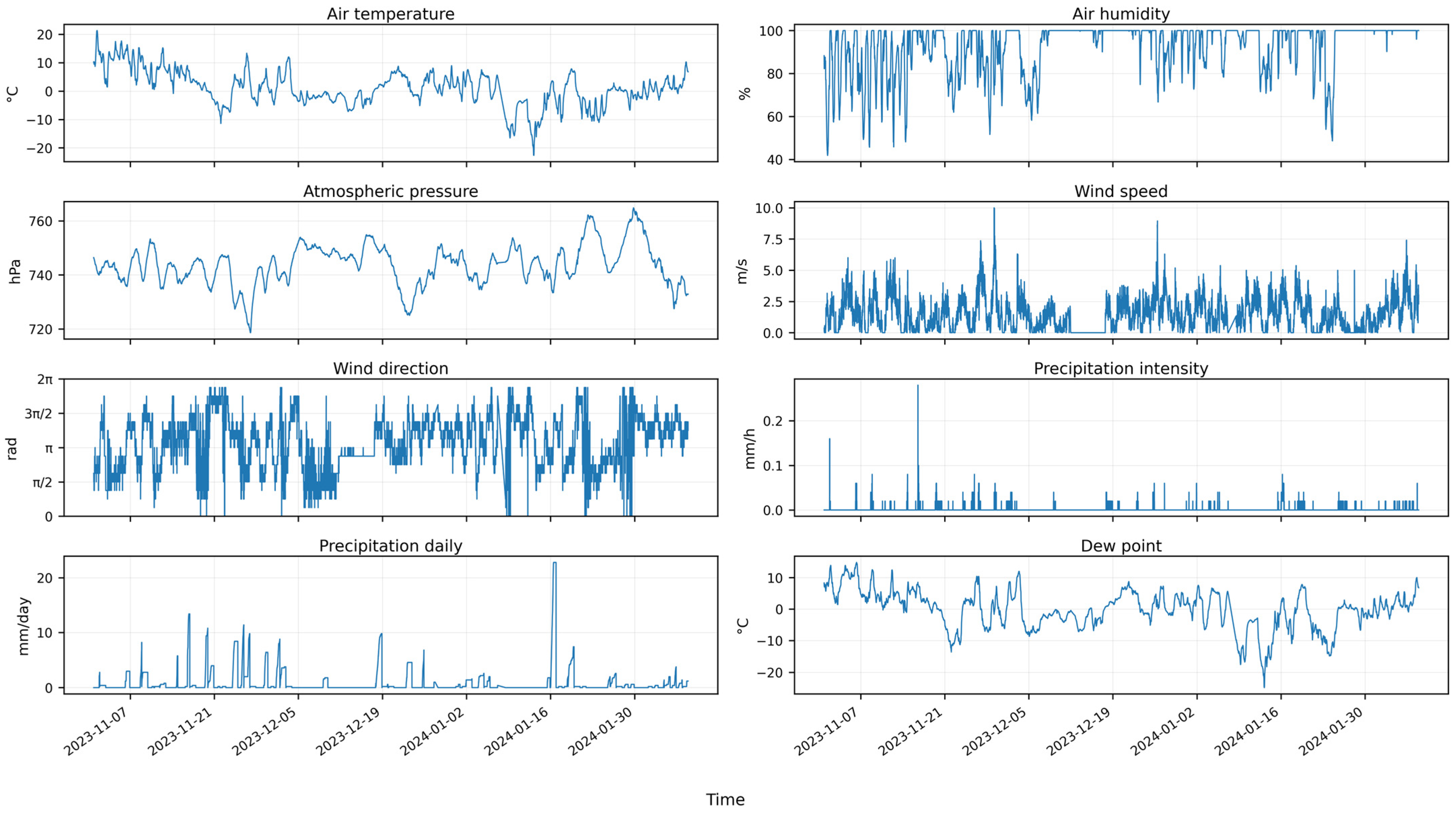
To provide a clear overview of the collected dataset, Figure 1 presents an eight-panel visualization, where each meteorological variable is shown on its own axis with its natural physical scale. This representation avoids the distortions of a single combined plot and allows each parameter: air temperature, relative humidity, atmospheric pressure, wind speed, wind direction, precipitation intensity, daily precipitation, and dew point, to be interpreted independently. The selected segment (November 2023–February 2024) is continuous and stable, allowing for a clean inspection of short-term dynamics and sensor behavior relevant to the forecasting task.

The raw dataset consisted of N = 58,802 time-stamped observations collected at a nominal sampling interval of Δt ≈ 10 min. The cleaned dataset contained no NaN values within the recorded measurement rows. However, the original monitoring timeline included natural timestamp gaps caused by field-level interruptions such as communication failures, power instability, or sensor downtime. Therefore, “no missing values” refers only to the absence of missing entries inside retained records, not to the absence of temporal gaps in the complete observation timeline. This distinction is important because the synthetic degradation experiments introduced controlled missingness into the retained data matrix, whereas naturally occurring timestamp gaps were treated as part of the field acquisition context. Figure 1 focuses on a continuous stable segment; the full dataset still contains natural timestamp gaps caused by field-level operational interruptions.

The plots use the following axis labels and units: air temperature (°C), air humidity (%), atmospheric pressure (hPa), wind speed (m/s), wind direction (rad), precipitation intensity (mm/h), daily precipitation (mm/day), and dew point (°C). Wind direction is shown in radians in Figure 1 only for physical interpretability of the original measurement. In the machine-learning pipeline, however, wind direction was represented by its sine and cosine components rather than by the raw angular value.

Initial data cleaning was performed according to three quality-control principles: temporal consistency, physical plausibility, and preservation of causal structure. First, duplicated timestamps and repeated measurement rows were removed to ensure that each observation corresponded to a unique time point in the monitoring sequence. Second, measurements outside physically meaningful ranges were treated as invalid sensor artefacts rather than as extreme meteorological events. Specifically, relative humidity values below 0% or above 100% were removed; temperature readings below −40 °C or above 60 °C were discarded as implausible for the considered field conditions and sensor specifications; and negative wind-speed values were excluded because wind speed is a non-negative physical quantity.

Third, isolated single-point spikes were treated separately from sustained meteorological changes. Abrupt one-sample deviations that were not supported by adjacent observations were interpreted as transient artefacts caused by electrical interference, communication instability, or short-term sensor malfunction. These isolated spikes were smoothed using a three-point median window, which suppresses local outliers while preserving short-term trends and abrupt but persistent atmospheric changes.

In a real continuous operation scenario, outliers would be handled causally at the edge/fog preprocessing stage rather than using future observations. Each incoming measurement would first be checked against physically plausible limits for the corresponding meteorological variable. In addition, isolated one-step deviations would be detected using a rolling median and local variability estimated only from the preceding observations in the current temporal block. If an observation exceeded the physical plausibility range or strongly deviated from the recent local pattern, it would be flagged as a potential outlier. Such values would not be used directly for lag construction; instead, they would be replaced by a causal rolling median or the most recent valid observation when the local history is insufficient. The outlier flag itself can also be retained as a data-quality indicator for future deployment-oriented studies. This approach prevents future data leakage and keeps the forecasting pipeline operational during transient sensor spikes, electrical interference, or short communication artifacts.

The cleaning procedure was applied before feature generation and before the synthetic degradation experiments. Naturally occurring timestamp gaps caused by field-level interruptions were retained as part of the acquisition context, whereas controlled missingness was introduced later during the robustness experiments. No future observations or target values were used during cleaning, imputation, or feature construction, thereby preserving the causal structure required for one-step-ahead edge/fog forecasting.

To enable compatibility with supervised machine-learning models, the data were transformed into a lag-embedded representation. For each time series, lagged features were generated for the preceding six observation intervals:

$$(x_{t-1},x_{t-2},\dots ,x_{t-6})$$

(1)

where $x_t$ is the value of a meteorological variable at time $t$; $x_{t-k}$ is its value at lag $k$; and $k\in \{1,\dots ,6\}$ defines the one-hour temporal window capturing short-term dependencies essential for forecasting.

Capturing short-term temporal dependencies is essential for one-step-ahead forecasting. The choice of six lags was guided by empirical inspection of the autocorrelation (ACF) and partial autocorrelation (PACF) functions, both of which indicated that the strongest dependencies are concentrated within the preceding hour (≈60 min). This lag depth offers a favorable trade-off between predictive accuracy and model complexity: adding additional lags did not significantly improve performance but increased memory requirements and inference latency, both of which are undesirable for resource-constrained fog and/or edge environments.

In addition to lagged values, causal rolling descriptors were computed to encode short-term variability and local atmospheric dynamics. To prevent information leakage, all moving averages and moving standard deviations were calculated only from observations available before the prediction instant. In implementation terms, the time series was shifted by one step before applying rolling-window operations. Thus, for a forecast issued at time $t$, the feature vector used observations up to $t-1$, while the target corresponded to the next observation. No centered rolling windows or future values were used.

Rolling statistics were computed over windows of 3, 6, and 12 previous observations, corresponding approximately to 30, 60, and 120 min under the nominal 10 min sampling interval. Near the beginning of each temporal block, samples with insufficient history were removed rather than filled using future information. This preserves the causal structure required for realistic edge inference.

Temporal gaps were handled before constructing lagged and rolling features. After sorting all records by timestamp, consecutive observations were grouped into continuous temporal blocks according to the nominal 10 min sampling interval. If the time difference between two neighbouring records exceeded the expected sampling interval, the sequence was treated as interrupted, and a new temporal block was started. Lagged features and rolling descriptors were then computed only within each continuous block. Therefore, observations before a temporal interruption were not used as lagged predictors for observations after the interruption. Samples at the beginning of each new block that did not have sufficient previous observations for the required six-lag window or rolling statistics were removed from the supervised learning matrix. This procedure prevents artificial temporal continuity across field-level communication or power gaps.

Moving averages capture local trends and smooth small-scale oscillations, whereas moving standard deviations quantify short-term variability and turbulence-like fluctuations. For each variable, these operations generated a set of temporal features that summarized the local structure of the signal.

By combining lagged observations and local statistical descriptors, the input feature vector for time $t$ takes the form:

$$z_t=[x_{t-1},x_{t-2},\dots ,x_{t-L},{\mathrm{MA}}_3(x_t),{\mathrm{MA}}_6(x_t),{\mathrm{MA}}_{12}(x_t),{\mathrm{SD}}_3(x_t),{\mathrm{SD}}_6(x_t),{\mathrm{SD}}_{12}(x_t\left)\right]$$

(2)

where $z_t$ is the feature vector at time $t$, $L$ is the number of lagged values, ${\mathrm{MA}}_w\left(x_t\right)$ and ${\mathrm{SD}}_w\left(x_t\right)$ are the moving average and moving standard deviation computed over a window $w\in \{3,6,12\}$, and each transformation is applied independently to every meteorological variable.

The physical dataset contains eight meteorological variables. However, after sine–cosine encoding of wind direction, the supervised modelling matrix contains nine modelled components because the raw wind-direction angle is represented by two variables: sin (θ) and cos (θ). Therefore, the feature-vector dimensionality was computed using the number of modelled components rather than only the number of original physical variables:

$$m=d\cdot L+6d$$

(3)

where $m$ is the dimensionality of the feature vector, $d$ is the number of modelled components after circular encoding, $L$ is the number of lag features per variable, and $6d$ corresponds to the statistical descriptors added for each variable.

The one-step-ahead forecasting task is defined as predicting the next multivariate observation:

$$y_t=x_{t+1}$$

(4)

where $y_t$ denotes the next-step target value and $x_{t+1}$ is the true observation one time step ahead, which is a standard formulation for real-time predictive control in edge computing, where forecasts must be updated continuously at the device level.

A machine-learning model is represented as follows:

$$f_{\phi }:{\mathbb{R}}^m\to {\mathbb{R}}^d$$

(5)

where $f_{\phi }$ is a machine-learning model parameterized by $\phi$, ${\mathbb{R}}^m$ is the input feature space, and ${\mathbb{R}}^d$ is the output space of predicted meteorological variables, parametrized by φ, which is trained to approximate the mapping from lagged features $z_t$ to the future state $y_t$.

To avoid temporal leakage, all experiments were conducted using chronological splitting. The dataset was ordered by timestamp before feature generation and model evaluation. The earliest observations were used for training, the subsequent temporal block was used for validation and hyperparameter selection, and the final temporal block was held out exclusively for testing. Specifically, the split was defined as follows: the first 70% of chronologically ordered observations were used for training, the following 15% for validation, and the final 15% for testing. No random shuffling was applied at any stage.

All preprocessing operations that require parameter estimation, including scaling and model fitting, were fitted only on the training block and then applied to validation and test blocks. Hyperparameters were selected using the validation block only, and the final reported performance was computed on the temporally held-out test block.

For robustness analysis, the same chronological protocol was preserved across all degradation scenarios. Synthetic missingness and noise were introduced after defining the temporal blocks, so that information from the validation or test periods could not affect training-time preprocessing. This design ensures that the evaluation reflects a causal one-step-ahead forecasting setting rather than an optimistic, randomly shuffled regression task:

$${\phi }^{*}=\mathrm{a}\mathrm{r}\mathrm{g} \underset{\phi }{\mathrm{m}\mathrm{i}\mathrm{n}}{\displaystyle \frac{1}{N}}{\displaystyle \sum _{t=1}^N}\parallel y_t-f_{\phi }\left(z_t\right){\parallel }^2$$

(6)

where ${\phi }^{*}$ are the optimal model parameters, $N$ is the number of training samples, $y_t$ is the ground-truth target, $f_{\phi }\left(z_t\right)$ is the predicted value, and $\parallel \cdot {\parallel }^2$ is the squared Euclidean norm, with time-series-consistent splitting, ensuring that training and validation sets respect chronological order.

The formulation is generic and applies uniformly to all models evaluated in this study, including linear regressors, ensemble methods, and kernel-based predictors. To emulate the operational constraints of fog and/or edge devices, only a short rolling buffer representing a fraction $\alpha =0.10$ of the most recent samples was used for training:

$$D_{\mathrm{train}}=\left\{\right(z_t,y_t)\mid t\in [T(1-\alpha ),T\left]\right\}$$

(7)

where $D_{\mathrm{train}}$ is the training subset, $T$ is the total number of time steps, and $\alpha$ is the retained fraction of the most recent observations reflecting memory limits of fog/edge devices, and $T$ denotes the total number of time steps.

This setup reflects realistic memory limitations of embedded IoT gateways, which typically retain only short historical windows due to limited RAM and a lack of persistent storage.

Three forms of data degradation were modelled to replicate common real-world sensor failure modes. Missing-value corruption was introduced via a Bernoulli masking process:

$${\tilde{z}}_t=M_t\odot z_t,M_t\sim \mathrm{Bernoulli}(1-p_{\mathrm{miss}})$$

(8)

where ${\tilde{z}}_t$ is the masked feature vector, $M_t$ is the binary mask, $p_{\mathrm{miss}}$ is the missing-data probability, and $\odot$ denotes element-wise multiplication simulating signal loss or packet drop, mimicking the effects of intermittent wireless connectivity, packet loss, or power fluctuations. Additive measurement noise was simulated as Gaussian perturbations:

$${\tilde{z}}_t=z_t+{\epsilon }_t,{\epsilon }_t\sim \mathcal{N}(0,{\sigma }^{2}I)$$

(9)

where ${\tilde{z}}_t$ is the noise-corrupted feature vector, ${\epsilon }_t$ is Gaussian noise, ${\sigma }^2$ is noise variance, and $I$ is the identity matrix, assuming independent noise across all feature dimensions, representing sensor drift, thermal noise, and short-term electrical interference.

The Combined scenario applied both operators simultaneously, reflecting the multifaceted degradation typical of field-deployed meteorological stations.

In summary, the forecasting task evaluates degradation-tolerant mapping under noisy measurements, partial observation loss, and restricted historical data availability. The results are intended to inform future low-latency and memory-efficient edge/fog implementations, but they do not by themselves constitute hardware-level deployment validation.

To mimic restricted local-history availability in edge/fog monitoring systems, the reduced-history scenario used only the most recent fraction of the training observations. The most constrained case was defined as training-history fraction = 0.10, corresponding to approximately 5880 raw observations from the original dataset, or about 41 days of measurements at the nominal 10 min sampling interval. This value was selected as a conservative lower-bound stress test rather than as an exact memory specification of a single device. It reflects a realistic situation in which a microcontroller-class acquisition node performs local buffering and preprocessing, while a gateway-class edge/fog device retains only a limited recent history for model updating, rather than storing the full long-term archive. Therefore, the 10% case is used to evaluate how strongly each model depends on historical data availability under constrained local-buffer conditions.

Feature engineering, scenario generation, and model pipelines were implemented in Python using pandas, numpy, scikit-learn, and joblib. These libraries represent standard tools for high-quality time-series ML research.

Experiments were conducted offline in a Python 3 environment using pandas, NumPy, scikit-learn, and joblib on a CPU-based workstation with the following configuration: Intel Core i7-12700H processor, x86_64 architecture, 14 cores (6 performance + 8 efficiency cores) and 20 logical threads, 32 GB RAM, and a 64-bit Windows operating system. No GPU acceleration was used during model training or evaluation. Therefore, the reported results primarily characterize predictive accuracy and robustness under controlled degradation scenarios on offline CPU hardware. They should not be interpreted as direct evidence of deployment feasibility on specific embedded devices. Hardware-level validation, including inference latency, memory footprint, throughput, and energy consumption on representative edge/fog platforms, remains necessary before operational deployment.

The software environment used for the experiment was re-checked directly from the execution environment to ensure reproducibility. The experiments were conducted in Python 3.11.3 on a 64-bit Windows environment. The verified package versions were as follows: pandas 2.2.2, NumPy 1.26.4, SciPy 1.15.2, scikit-learn 1.6.1, joblib 1.4.2, threadpoolctl 3.5.0, and matplotlib 3.8.3. These versions were confirmed using pip freeze and scikit-learn’s show_versions() utility. The same software environment was used for preprocessing, feature engineering, model training, and evaluation across all experimental scenarios. The complete package list can be provided as a requirements file to support reproducibility.

The evaluated models include Ridge Regression, ElasticNet, Lasso, MultiTaskElasticNet, PLSRegression, Support Vector Regression (RBF kernel), Linear SVR, KNN, Random Forest, Extra Trees, Gradient Boosting, and HistGradientBoosting. This selection covers the main families of classical regression models relevant to robustness-oriented environmental forecasting, including regularized linear models, kernel-based methods, instance-based learning, and ensemble tree-based methods. The methodological basis of these families is supported by foundational studies on Random Forests [16], Support Vector Regression [17], Ridge Regression [18], Gradient Boosting [19], and efficient boosting frameworks such as LightGBM [20]. Recent sensor analytics studies also support the relevance of boosting-based models for environmental and energy-related sensor-data applications [21]. In agricultural sensing applications, recent reviews confirm the broader role of IoT- and AI-based monitoring systems in smart agriculture [1,2], while related local studies have applied machine-learning methods to crop-disease risk prediction, IoT decision-making networks, and weather-driven agricultural decision-support systems [22,23]. More broadly, recent reviews of machine-learning methods for time-series prediction and IoT–ML integration in precision agroecology further support the need for robustness-aware benchmarking of computationally efficient models for sensor-driven agricultural forecasting [24,25]. Considering these findings and the constraints of low-power embedded hardware, this set of algorithms represents a well-justified and practical choice for edge and/or fog-based agroclimatic forecasting.

The choice of the twelve models was based on a representative-family selection strategy rather than on an exhaustive enumeration of all possible forecasting algorithms. The selected models cover the main classes of classical regression methods that are practically relevant for deployment-oriented agroclimatic forecasting: regularized linear models, latent-variable regression, kernel-based regressors, instance-based learning, and ensemble tree-based methods. This selection makes it possible to compare models with different assumptions, complexity levels, bias–variance behavior, and expected robustness to degraded sensor data.

Four criteria guided the model selection. First, all models are available in lightweight and reproducible Python/scikit-learn pipelines, which is important for deployment-oriented edge/fog workflows. Second, the set includes both low-complexity models suitable for fast inference and more flexible nonlinear models capable of capturing interactions between meteorological variables. Third, the models differ in their expected sensitivity to missing values, additive noise, reduced training history, and combined degradation, which directly aligns with the study’s objective. Fourth, the selected models are commonly used as practical baselines or robust alternatives in environmental, agroclimatic, and IoT-oriented regression tasks.

Thus, the number twelve results from covering the major classical regression families while keeping the benchmark computationally manageable and methodologically consistent. Deep learning, hybrid statistical–neural, and specialized TinyML models were not included because the purpose of the present study is to provide an internal robustness benchmark for classical ML regressors under the same degradation protocol; broader cross-family comparisons are left for future work. The rationale for selecting the twelve classical machine-learning models is summarized in

Table 3. Rationale for selecting the twelve classical machine-learning models.

Model Family	Included Models	Reason for Inclusion
Regularized linear models	Ridge Regression, Lasso, ElasticNet, MultiTaskElasticNet	Fast, interpretable, low-complexity models suitable as lightweight baselines for edge/fog inference
Latent-variable regression	PLSRegression	Useful for multicollinear meteorological variables and compact multivariate representation
Kernel-based models	SVR, LinearSVR	Included to test margin-based regression under linear and nonlinear assumptions
Instance-based learning	KNN	Provides a non-parametric local baseline but is expected to be sensitive to storage and data degradation
Ensemble tree-based models	Random Forest, Extra Trees, Gradient Boosting, HistGradientBoosting	Included to evaluate nonlinear interactions, robustness to degraded data, and stability under noisy conditions

.

The ML models evaluated in this study were configured exactly as implemented in the experiment pipeline. Hyperparameter values were selected using a constrained configuration strategy rather than an exhaustive search. The goal was to compare model families under computationally realistic settings suitable for deployment-oriented analysis. Therefore, the selected values reflect commonly used stable configurations in scikit-learn and moderate model sizes that avoid excessive memory and inference costs. This design favors reproducibility and practical comparability, but it does not claim that each model was individually optimized to its maximum possible performance. Consequently, the reported results should be interpreted as a comparison of practical model configurations rather than as a fully exhaustive hyperparameter-optimization study.

All remaining parameters not listed in

Table 4. Hyperparameter settings used for the evaluated machine-learning models.

Model	Preprocessing	Hyperparameters Used
Ridge Regression	StandardScaler	alpha = 1.0; fit_intercept = True; solver = auto
Lasso	StandardScaler	alpha = 1.0; fit_intercept = True; max_iter = 1000; tol = 1 × 10−4
ElasticNet	StandardScaler	alpha = 1.0; l1_ratio = 0.3; fit_intercept = True; max_iter = 1000; tol = 1 × 10−4
MultiTaskElasticNet	StandardScaler	alpha = 1.0; l1_ratio = 0.3; fit_intercept = True; max_iter = 1000; tol = 1 × 10−4
PLSRegression	StandardScaler	n_components = 8
SVR	StandardScaler	kernel = RBF; C = 3.0; epsilon = 0.1; gamma = scale
LinearSVR	StandardScaler	C = 2.0; epsilon = 0.0; loss = epsilon_insensitive; max_iter = 1000
KNN	StandardScaler	n_neighbors = 5; weights = uniform; metric = minkowski; p = 2
Random Forest	None	n_estimators = 100; max_depth = None; min_samples_split = 2; min_samples_leaf = 1; random_state = fixed
Extra Trees	None	n_estimators = 100; max_depth = None; min_samples_split = 2; min_samples_leaf = 1; random_state = fixed
Gradient Boosting	None	n_estimators = 100; learning_rate = 0.1; max_depth = 3; subsample = 1.0; random_state = fixed
HistGradientBoosting	None	max_iter = 100; learning_rate = 0.1; max_leaf_nodes = 31; l2_regularization = 0.0; random_state = fixed

were kept at their default scikit-learn values. This table is included to ensure reproducibility of the benchmark and to clarify that the comparison was based on fixed practical configurations rather than on exhaustive model-specific hyperparameter optimization.

Linear and kernel-based models were also included: SVR with an RBF kernel (C = 3.0), LinearSVR (C = 2.0), and PLSRegression with 8 latent components for extracting the multivariate structure. Additionally, ElasticNet and MultiTaskElasticNet were evaluated with l1_ratio = 0.3 to balance L1/L2 regularization. KNN was implemented with 5 neighbors. Models sensitive to feature scaling (Ridge, ElasticNet, Lasso, MultiTaskElasticNet, PLSRegression, SVR, LinearSVR, and KNN) were implemented via pipelines with StandardScaler to ensure numerical stability during training.

For each evaluated model and degradation scenario, the following standard forecasting metrics were computed on the temporally held-out test block:

$$\mathrm{MAE}={\displaystyle \frac{1}{n}}{\displaystyle \sum _{i=1}^n}\mid y_i-{\widehat{y}}_i\mid$$

(10)

where $n$ is the number of samples, $y_i$ is the true value, and ${\widehat{y}}_i$ is the predicted value.

$$\mathrm{RMSE}=\sqrt{{\displaystyle \frac{1}{n}}{\displaystyle \sum _{i=1}^n}(y_i-{\widehat{y}}_i{)}^2}$$

(11)

where RMSE is the root mean squared error computed from $n$ true-predicted pairs.

$$R^2=1-{\displaystyle \frac{\sum {(y_i-{\widehat{y}}_i)}^2}{\sum {(y_i-\bar{y})}^2}}$$

(12)

where $R^2$ is the coefficient of determination, $\bar{y}$ is the true-value mean, and the numerator and denominator represent the model error and total variance respectively.

These metrics reflect absolute error, penalization of large deviations, and the proportion of explained variance. For wind direction, circular error metrics were used instead of ordinary linear errors on raw radians. The angular prediction error was computed as the shortest circular distance between the observed angle θ_true and the reconstructed predicted angle θ_pred:

e_angle = |((θ_pred − θ_true + π) mod 2π) − π|.

(13)

Circular MAE and circular RMSE were then computed from this angular error. For R²-based comparison, wind-direction performance was represented in the sine–cosine component space by averaging the R² values obtained for the predicted sine and cosine components.

Because the absolute values of MAE, RMSE, and R² differ substantially across meteorological parameters and because wind direction requires circular treatment, the heatmaps presented in the Results section use normalized rather than raw metric values. Normalization was performed independently for each target variable and each metric across the evaluated models. For an error metric E ∈ {MAE, RMSE}, the normalized value for model i and target variable j was computed as follows:

$$E_{norm}(i,j)={\displaystyle \frac{E(i,j)-\underset{i}{\mathrm{m}\mathrm{i}\mathrm{n}} E(i,j)}{\underset{i}{\mathrm{m}\mathrm{a}\mathrm{x}} E(i,j)-\underset{i}{\mathrm{m}\mathrm{i}\mathrm{n}} E(i,j)}}$$

(14)

Thus, E_norm = 0 corresponds to the lowest error for a given target variable, whereas E_norm = 1 corresponds to the highest error. For R², the normalized value was computed as follows:

$$R_{\mathrm{norm}}^2(i,j)={\displaystyle \frac{R^2(i,j)-\underset{i}{\mathrm{m}\mathrm{i}\mathrm{n}} R^2(i,j)}{\underset{i}{\mathrm{m}\mathrm{a}\mathrm{x}} R^2(i,j)-\underset{i}{\mathrm{m}\mathrm{i}\mathrm{n}} R^2(i,j)}}$$

(15)

where higher normalized values indicate stronger predictive performance. This column-wise normalization makes it possible to compare the relative ranking of models within each meteorological target while avoiding dominance by variables with larger physical scales or variances. The absolute numerical results remain available in the dataset and are used in the quantitative analysis.

Wind direction was treated as a circular variable throughout the modelling and evaluation pipeline. Because angular values close to 0 and 2π radians are physically adjacent but numerically distant, direct regression on raw radian values may distort model training and ordinary error metrics. Therefore, the raw wind-direction angle θ was transformed into two circular components before supervised learning:

wind_dir_sin = sin(θ);

wind_dir_cos = cos(θ).

The models were trained to predict these two components instead of the raw angular value. After prediction, wind direction was reconstructed using the two-argument arctangent function:

wind_dir_pred = atan2(wind_dir_sin_pred, wind_dir_cos_pred),

and then mapped to the [0, 2π) interval. Wind-direction errors were evaluated using the shortest circular angular distance between the observed and reconstructed predicted angles. This procedure prevents physically adjacent directions near the 0/2π boundary from being treated as large numerical errors.

To evaluate robustness under realistic IoT conditions, the following scenarios were simulated:

• Baseline: clean data without degradation.
• Noise: added white Gaussian noise with σ = 0.01–0.15.
• Missing Data: random removal of 5–30% of sensor readings followed by causal forward-fill imputation within each temporal block, limited to six consecutive observations; initial missing values or missing sequences exceeding this limit were replaced using statistics estimated from the training block only. This scenario represents packet loss and intermittent sensor failures.
• Reduced training-history fraction: training on 10–100% of the available historical data.
• Combined Distortion: simultaneous application of noise and missing data.

This experimental protocol addresses the core challenges of IoT and fog/edge sensing systems, including intermittent data, sensor drift, packet loss, and constrained computational budgets.

Forward-fill imputation was applied causally within each temporal block and was limited to a maximum of six consecutive missing observations, corresponding to approximately 60 min at the nominal 10 min sampling interval. This limit was selected to match the six-lag forecasting window used in the feature construction stage. Longer missing sequences were not propagated indefinitely by forward-fill; remaining unresolved missing values after this limit were replaced using statistics estimated from the training block only. This procedure prevents long artificial plateaus in the time series and avoids using future observations during imputation.

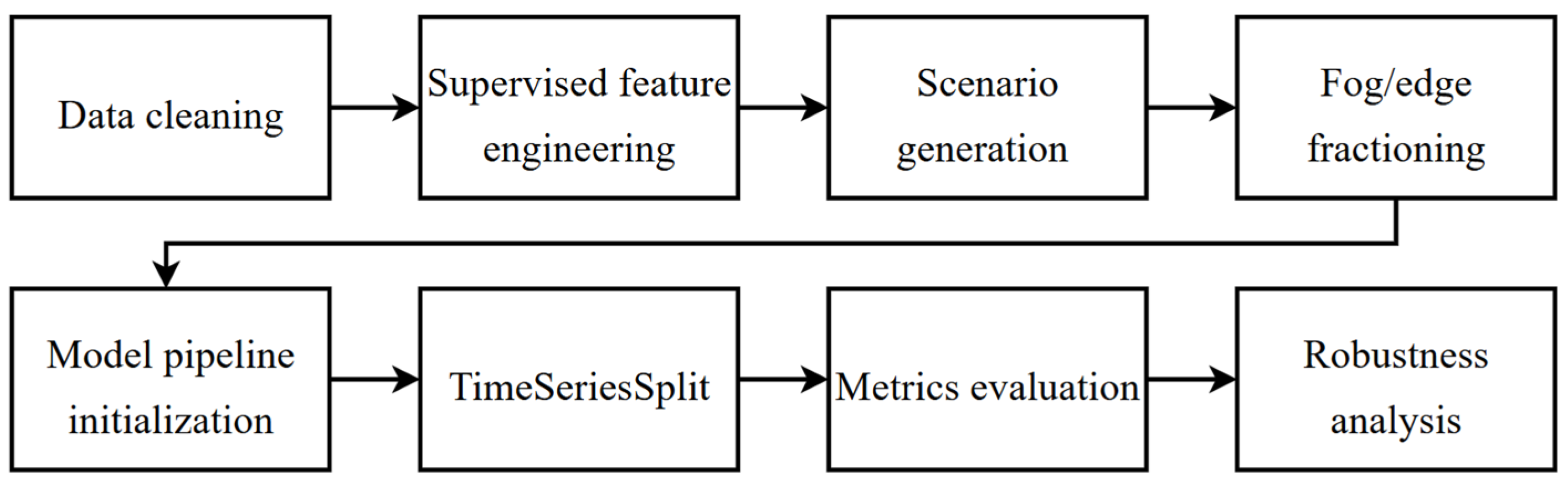
Figure 2 presents an overview of the full research workflow, including data acquisition, preprocessing, feature engineering, scenario simulation, model training, and evaluation. This structured pipeline reflects real fog and/or edge operational constraints and provides reproducible methodology for environmental time-series forecasting.

3. Results

To evaluate the performance and robustness of ML models under realistic fog/edge conditions, we constructed an experimental framework that simulates various types of data degradation commonly encountered in IoT sensor networks. The study includes five experimental scenarios: Baseline, Missing Data, Noise, Reduced training-history fraction, and Combined Distortion. These scenarios represent the most frequent causes of degradation in field-deployed monitoring systems, where sensors may experience packet loss, calibration drift, interference, and power-related inconsistencies. The five experimental degradation scenarios and their corresponding degradation mechanisms are summarized in

Table 5. Experimental degradation scenarios.

Scenario	Description
Baseline	Clean dataset without any artificial distortions. Serves as the reference for all comparisons.
Missing data	Random removal of 5–30% of sensor readings followed by causal forward-fill imputation within each temporal block, limited to six consecutive observations; initial or longer unresolved missing values were handled using statistics estimated from the training block only. Represents packet loss and intermittent sensor failures.
Noise	Addition of Gaussian noise with σ = 0.01–0.15 to simulate sensor drift and atmospheric interference.
Reduced training-history fraction	Restriction of the available training history to 10–100% of historical observations to emulate limited local storage in edge/fog systems.
Combined distortion	Simultaneous application of noise (σ = 0.05–0.1) and missing data (10–20%). Represents the most realistic conditions for IoT field applications.

.

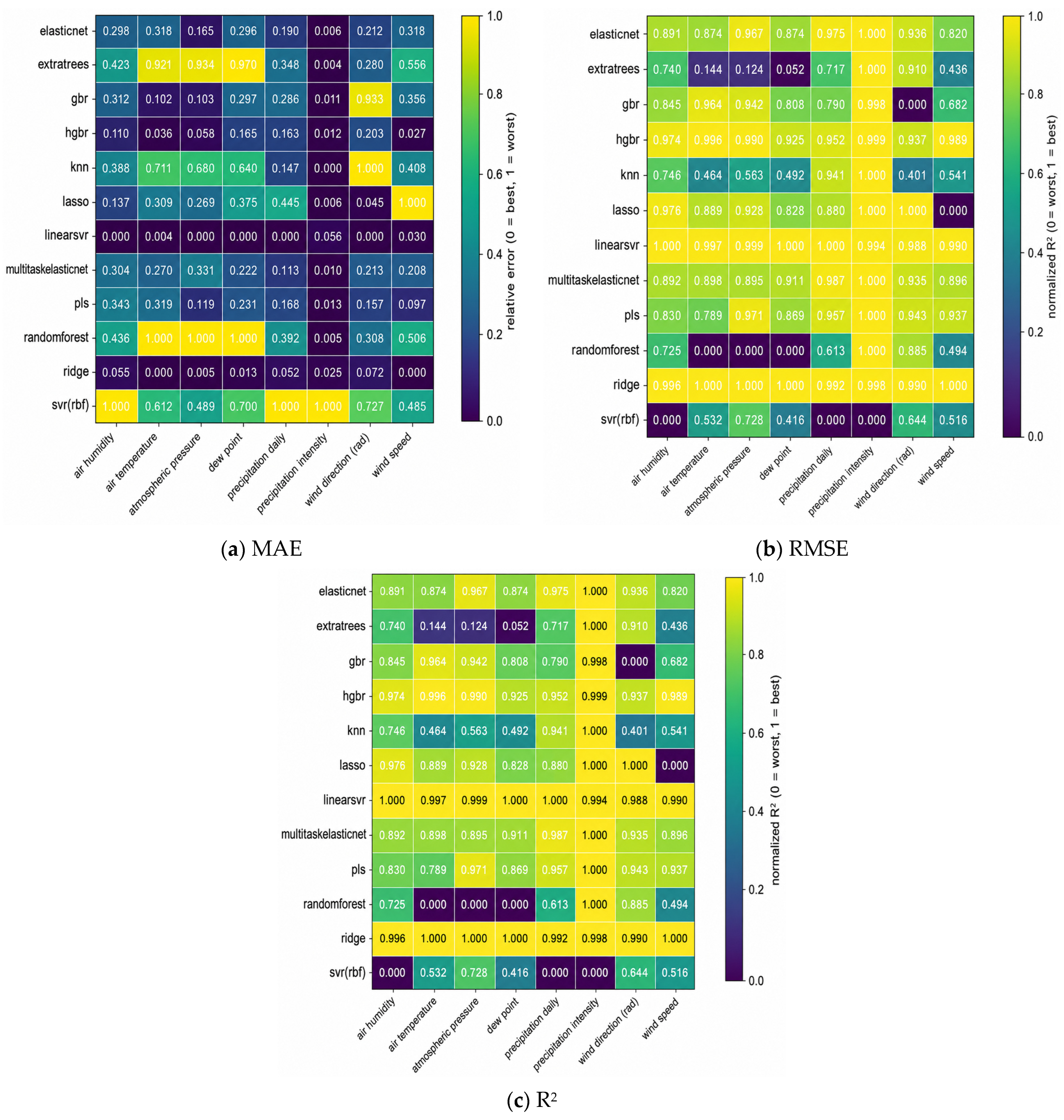
Figure 3 presents normalized MAE, RMSE, and R² heatmaps for the Baseline scenario. The normalization procedure used for these heatmaps is described in Section 2.

The color scale represents normalized model performance in the [0, 1] range. For wind direction, MAE and RMSE were computed as circular angular errors after sine–cosine encoding and angle reconstruction. The R² value for wind direction corresponds to the average R² of the sine and cosine components. Axis labels and units: air temperature (°C), air humidity (%), atmospheric pressure (hPa), wind speed (m/s), wind direction (rad), precipitation intensity (mm/h), daily precipitation (mm/day), and dew point (°C).

Under the Baseline scenario, wind direction was evaluated using sine–cosine encoding and reconstructed angular predictions. Unlike direct radian-based regression, this approach accounts for the circular nature of the variable and avoids artificial error inflation near the 0/2π boundary. Therefore, wind-direction results were included in the robustness-oriented evaluation using circular MAE/RMSE and sine–cosine component-based R².

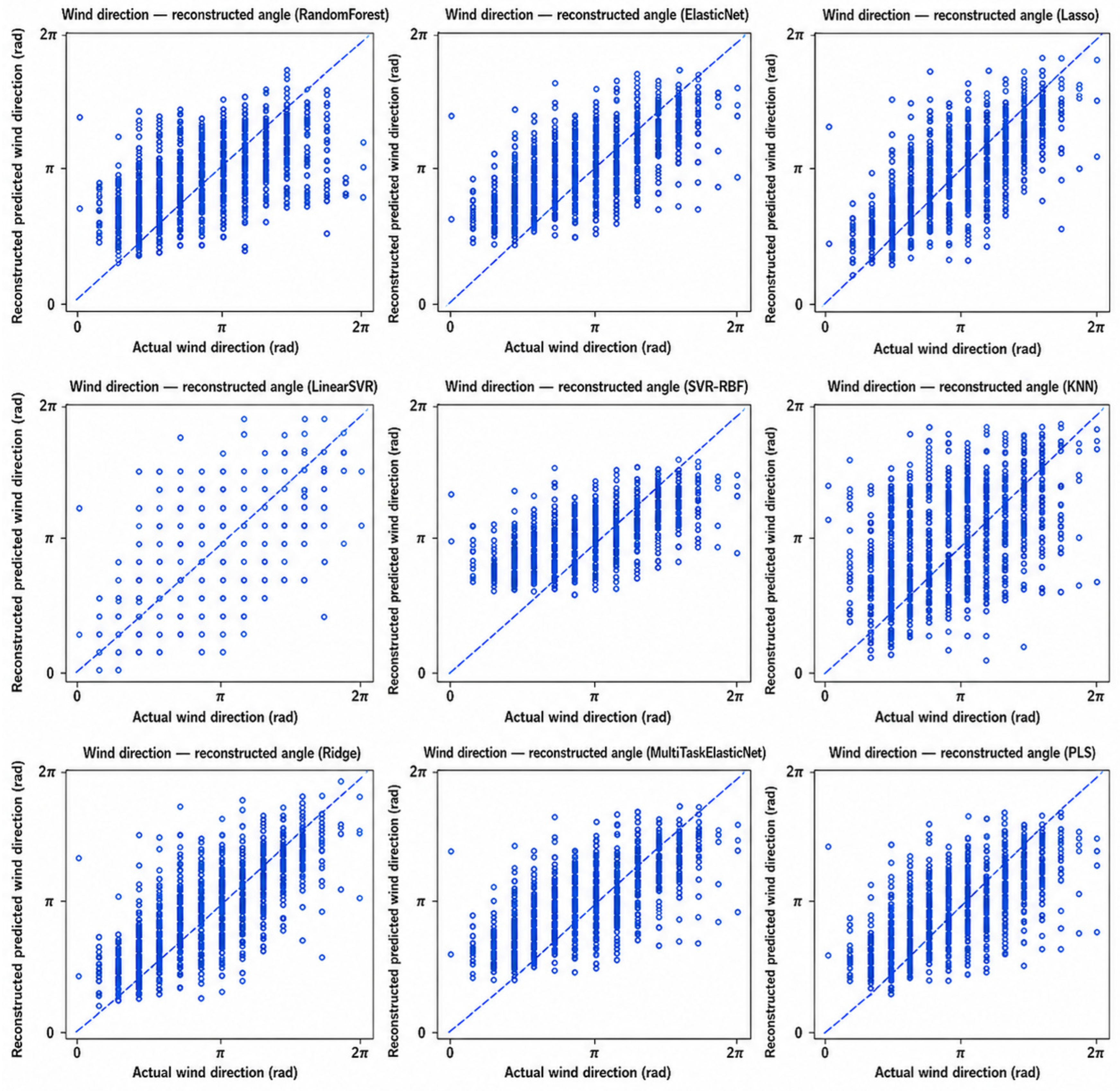
Figure 4 shows actual versus reconstructed predicted wind direction after sine–cosine encoding in the Baseline scenario. The predicted angular values were reconstructed from the predicted sine and cosine components using the inverse atan2 transformation. The quantitative evaluation of these predictions was based on the shortest circular angular distance between the observed and reconstructed predicted wind direction, rather than on ordinary linear differences between raw radian values.

Each panel shows reconstructed angular predictions obtained after sine–cosine encoding and inverse atan2 transformation. The horizontal axis corresponds to the observed wind direction, and the vertical axis corresponds to the reconstructed predicted wind direction, both expressed in radians. The dashed diagonal line denotes perfect agreement between observation and prediction. The evaluation of these predictions was based on circular angular error rather than ordinary linear error on raw radian values.

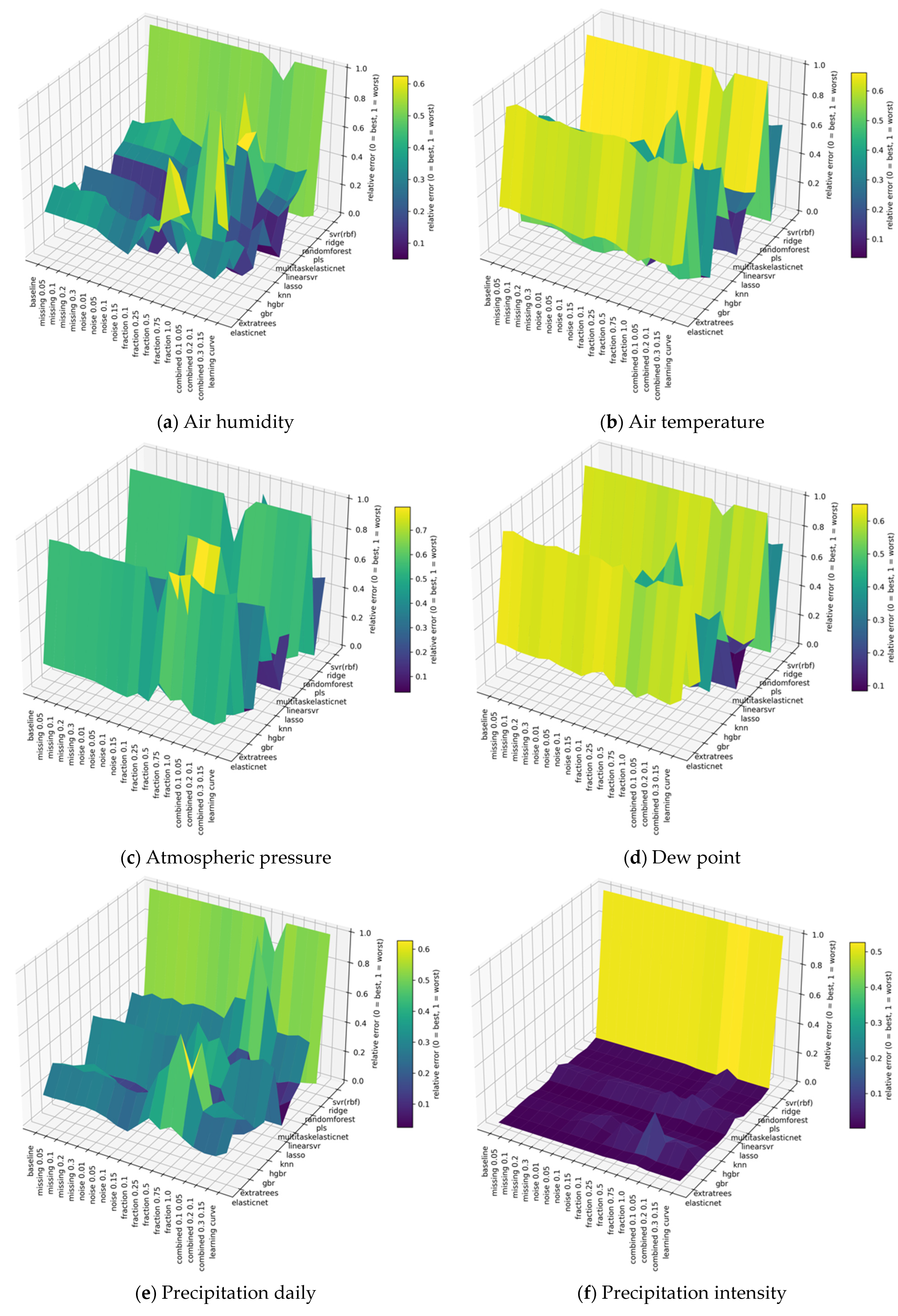
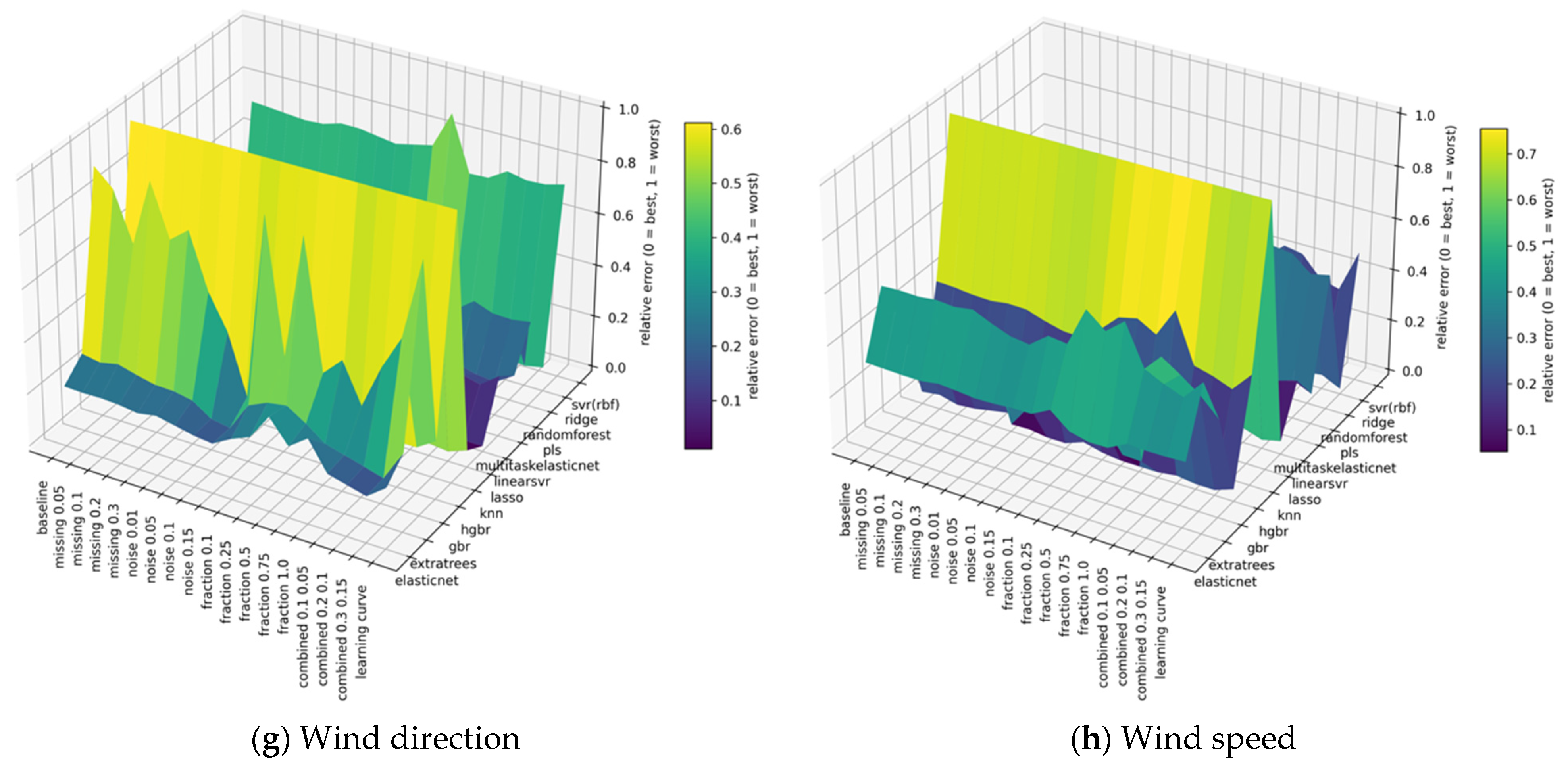
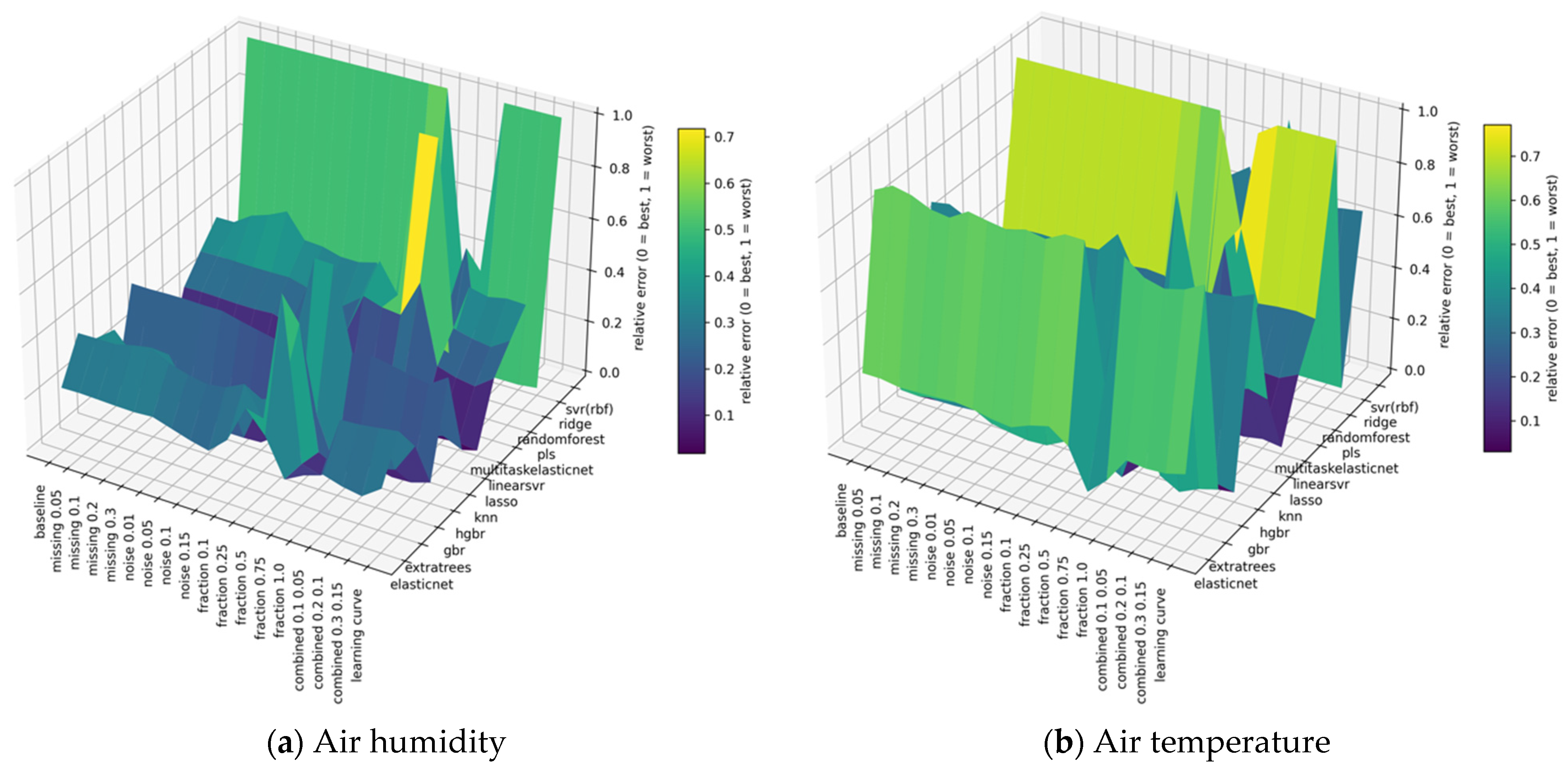
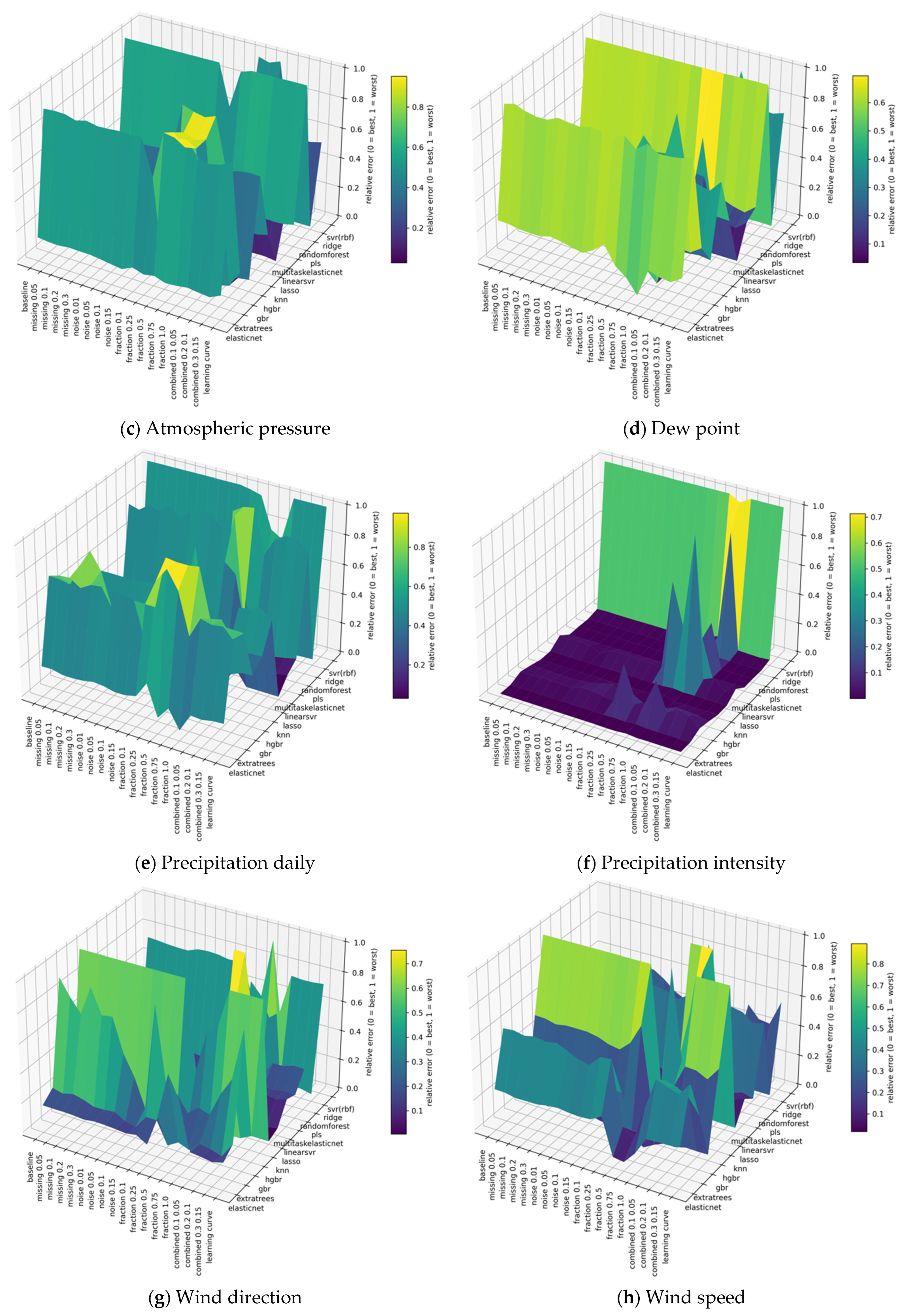
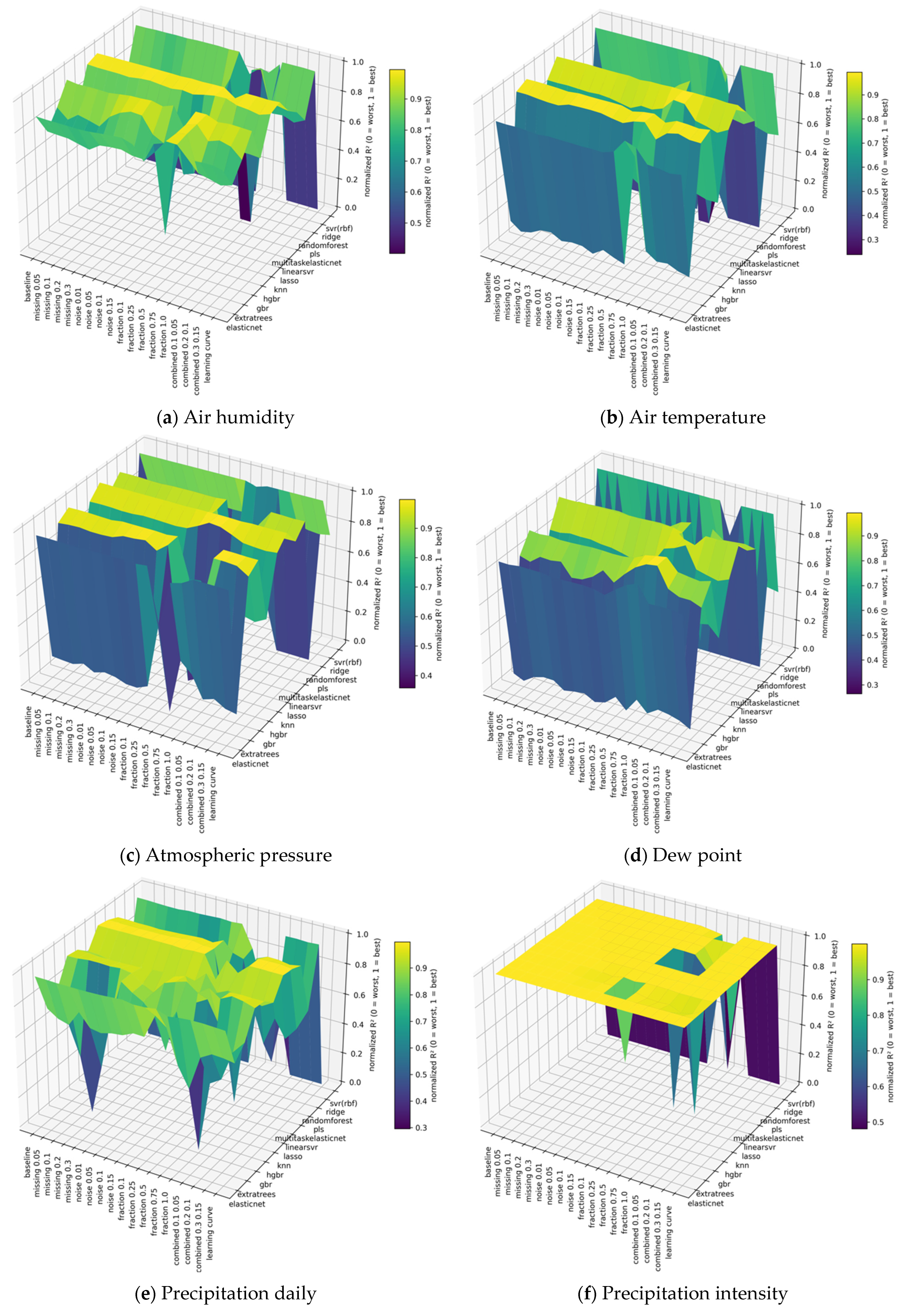
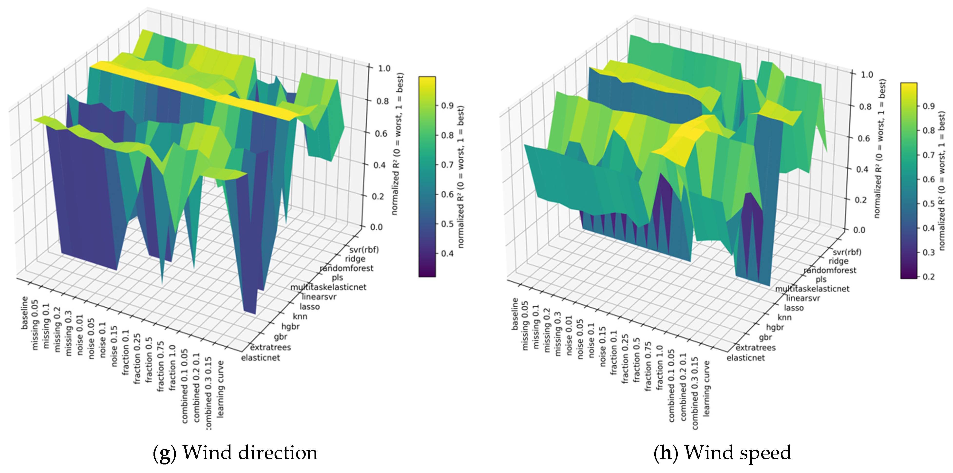
Figure 5, Figure 6 and Figure 7 summarize the relative normalized performance of the evaluated models across the five degradation scenarios: Baseline, Missing Data, Noise, Reduced training-history fraction, Combined Distortion, and the Baseline reference. The horizontal axis represents the degradation scenarios, the vertical axis represents the evaluated models, and the surface height represents the corresponding normalized metric value. For MAE and RMSE, lower values indicate lower relative error, whereas for R², higher values indicate stronger relative predictive performance. The notation used on the horizontal axis is as follows: baseline denotes clean reference data; missing x% corresponds to removal of x% of samples; noise σ denotes additive Gaussian perturbation with standard deviation σ; training-history fraction y% indicates training on y% of the available historical observations; and combined denotes simultaneous missing values and injected noise. For wind direction, MAE and RMSE surfaces are based on circular angular error after sine–cosine encoding and angular reconstruction. The R² surface for wind direction represents the average R² of the sine and cosine components.

In these surfaces, the horizontal axis represents the ordered sequence of degradation scenarios, including the Baseline reference and progressively more adverse Missing, Noise, Reduced training-history fraction, and Combined conditions. The vertical axis enumerates all evaluated machine-learning models, while the height and color of the surface encode the relative MAE on a normalized 0–1 scale, where lower values indicate better performance. Darker regions correspond to lower relative MAE values, whereas brighter regions correspond to higher relative MAE values under the corresponding scenario. This visualization summarizes the relative MAE values observed for each model under the evaluated degradation regimes.

Lower values indicate smaller absolute forecast errors and therefore better short-term predictive accuracy. Models positioned near the lower regions of the surface demonstrate stable performance across degradation scenarios, whereas higher regions correspond to larger relative MAE values under the corresponding scenario.

Here, the horizontal axis shows the degradation scenarios ordered from the Baseline to the most challenging Combined conditions, while the vertical axis lists the machine-learning models. The surface height and color reflect the normalized RMSE, expressed on a 0–1 scale in which lower values correspond to lower relative RMSE values. Dark continuous regions indicate models that maintain a low RMSE even when the data are corrupted or reduced, whereas higher regions indicate larger relative RMSE values under the corresponding degradation scenario. The surface summarizes the relative RMSE values across models and scenarios.

The relative RMSE highlights sensitivity to large deviations in the forecast. Lower values correspond to models that show lower relative RMSE values, while higher regions indicate larger relative RMSE values under specific degradation regimes. Because RMSE penalizes occasional large fluctuations more strongly than MAE, the surface shows where larger relative RMSE values were observed in the evaluated experimental grid.

In these plots, the horizontal axis denotes the full spectrum of degradation scenarios, and the vertical axis represents the set of evaluated models. The surface height and color encode the R² values on the 0–1 scale, where higher values reflect stronger predictive consistency and higher original R², whereas lower values correspond to degraded explanatory power. Higher regions correspond to higher relative R² values, whereas lower regions correspond to lower relative R² values.

Higher R² values indicate better variance preservation and stronger explanatory power of the model. Regions with low R² correspond to lower test-set explanatory performance under the corresponding scenario. The surface summarizes the observed R² variation across noise, missing-data, combined-distortion, and reduced-history scenarios.

In the Baseline condition, the lowest MAE and highest R² for temperature forecasting were obtained by regularized linear models, particularly Ridge Regression, which achieved an MAE of 0.318 and an R² of approximately 0.98. In the evaluated test configuration, this result indicates high one-step-ahead temperature forecasting accuracy for Ridge Regression under the selected lag-based feature representation. This interpretation should be restricted to the present dataset, forecast horizon, and feature construction strategy.

Under 5–15% missing values, Ridge Regression showed a smaller MAE increase, with MAE increasing by less than 10%. HistGradientBoosting surpassed Ridge only at higher missing rates (20–30%). Conversely, models such as SVR, KNN, and Random Forest showed lower R² values, with R² falling to zero or even becoming negative at 30% missing values, corresponding to substantially lower test-set performance under this degradation level.

When Gaussian noise with σ = 0.05–0.1 was injected into the dataset, both Ridge Regression and HistGradientBoosting maintained comparatively high test-set R² values, maintaining R² in the range of 0.95–0.97. In contrast, SVR and Random Forest showed lower test-set R² values, with negative R² values indicating worse performance than the naive mean prediction.

Ridge Regression achieved an R² value greater than 0.9 even when trained on only 50% of the available data, showing comparatively stable test-set performance under the reduced-history condition evaluated in this benchmark. RandomForest, ExtraTrees, and SVR showed lower test-set R² values when training data fell below 50%, reflecting their higher variance and sensitivity to limited datasets.

The Combined scenario produced the largest differences in test-set metrics among the evaluated models. Ridge remained effective for temperature and humidity, but for more volatile parameters (e.g., wind or precipitation), HistGradientBoosting outperformed it. Under the combined-degradation scenario with σ = 0.1 noise and 20% missing data, HistGradientBoosting achieved an R² value greater than 0.85 in the evaluated test configuration, whereas several alternative models showed substantially lower or even negative R² values. This result identifies HistGradientBoosting as the model with the most favorable metric profile for this combined-degradation test configuration. However, broader claims about its general superiority require validation across additional temporal folds, seasons, and external datasets.

To provide a compact comparison of all twelve evaluated models,

Table 6. Summary-level comparison of all evaluated machine-learning models.

Model	Model Family	Observed Behavior Across Scenarios	Observed Summary
Ridge Regression	Regularized linear model	Achieved the strongest baseline accuracy and remained stable under mild missingness, noise, and reduced training history	Lowest errors among the evaluated models under clean and mildly degraded conditions
Lasso	Regularized linear model	Demonstrated stable but generally less competitive performance than Ridge because stronger sparsity may remove useful lag features	Lower relative performance than Ridge Regression in the evaluated scenarios
ElasticNet	Regularized linear model	Provided balanced regularization and moderate robustness but did not outperform Ridge in the main scenarios	Moderate relative performance across the evaluated scenarios
MultiTaskElasticNet	Multivariate regularized linear model	Captured multi-output structure but showed no clear advantage over simpler regularized linear models	No clear metric advantage over simpler regularized linear models
PLSRegression	Latent-variable regression	Handled multicollinearity among meteorological variables but showed limited superiority under degradation	Lower robustness metrics than Ridge Regression or HistGradientBoosting in the evaluated scenarios
SVR	Kernel-based model	Performance deteriorated strongly under missingness, noise, and reduced training data	Lower relative performance under the tested degraded-data settings
LinearSVR	Linear margin-based model	More computationally practical than nonlinear SVR but still less stable than Ridge under several degradation settings	Lower relative performance than Ridge Regression in several degradation scenarios
KNN	Instance-based model	Sensitive to missingness, noisy inputs, and limited training history because prediction depends directly on local sample structure	Higher sensitivity to missingness, noise, and reduced training history in the evaluated scenarios
Random Forest	Ensemble tree-based model	Showed useful nonlinear capacity but degraded under strong missingness and reduced data availability	Higher metric deterioration under strong missingness and reduced-history scenarios
Extra Trees	Ensemble tree-based model	Provided nonlinear modeling ability but remained sensitive to scenario changes and did not consistently dominate	No consistent metric advantage over the leading models in the evaluated scenarios
Gradient Boosting	Ensemble boosting model	Demonstrated stronger structured learning than some baselines but was less consistently robust than HistGradientBoosting	Lower robustness metrics than HistGradientBoosting under severe degradation
HistGradientBoosting	Ensemble boosting model	Maintained the strongest robustness under severe missingness and combined noise–missingness degradation	Lowest relative error under severe combined degradation among the evaluated models

summarizes their observed behavior across the baseline and degradation scenarios. The table is intended as a results-oriented overview rather than as a replacement for the detailed metric-based figures. It summarizes the observed metric behavior of each model under the experimental conditions considered in this study.

As shown in Table 6, Ridge Regression and HistGradientBoosting obtained the most favorable metric profiles among the evaluated models. Ridge Regression showed lower errors under clean and mildly degraded conditions, whereas HistGradientBoosting showed lower relative error under severe missingness and combined degradation. SVR, KNN, Random Forest, and several other models showed higher sensitivity to degraded-data scenarios in the evaluated test configurations.

The leading models in

Table 7. Metric-based summary of leading models across experimental scenarios.

Scenario	Leading Model	Metric-Based Observation
Baseline	Ridge Regression	Lowest MAE and highest R2 among the evaluated models on clean data (MAE = 0.318; R2 ≈ 0.98).
Missing data	Ridge (≤15%), HGBR (>20%)	Ridge showed smaller metric changes at lower missing rates; HGBR showed lower relative errors at higher missing rates.
Noise	Ridge/HGBR	Maintained comparatively high R2 values under Gaussian noise σ = 0.05–0.1.
Reduced training-history fraction	Ridge Regression	Maintained R2 > 0.9 when trained on 50% of the available historical data.
Combined distortion	HistGradientBoosting	Lowest relative error in the evaluated combined-degradation test configuration; maintained R2 > 0.85 under combined noise + missing data.

were selected using a metric-based ranking procedure computed on the temporally held-out test block. For the Baseline scenario, the primary criteria were the lowest MAE and RMSE, together with the highest R². For Missing Data, Noise, and Combined Distortion scenarios, model selection additionally considered robustness, defined as the smallest relative deterioration of MAE/RMSE and the strongest preservation of R² compared with the Baseline condition. For the reduced training-history fraction scenario, priority was given to models that maintained high R² and low error values under reduced training-history availability. When two models showed comparable metric values, preference was given to the simpler or more stable model across adjacent degradation levels. Therefore, the term “leading model” refers to metric-based robustness within the evaluated experimental grid and does not imply statistical significance beyond the reported test-set metrics.

The scenario-dependent model rankings summarized in Table 7 show that Ridge Regression had the most favorable metric profile under clean or mildly degraded conditions, whereas HistGradientBoosting had the most favorable metric profile under severe combined degradation. The practical interpretation of these findings is discussed in Section 4.

4. Discussion and Prospects for Further Research

The experimental evaluation demonstrates that different ML models exhibit distinct strengths depending on the type and severity of data degradation, which is a crucial characteristic for real-world fog/edge deployments, where sensors frequently produce incomplete or noisy data. Among the evaluated models, Ridge Regression [18] consistently achieved the highest accuracy on clean or mildly corrupted data. Its stability under low to moderate levels of degradation (≤15% missing values and moderate Gaussian noise) suggests that the short-term meteorological dependencies captured by the lag-based feature space exhibit a predominantly linear structure. This observation aligns with prior studies, which have shown that environmental variables with high temporal autocorrelation are effectively modeled using regularized linear approaches.

The sine–cosine representation of wind direction reduced the methodological distortion caused by the circular discontinuity at 0/2π radians. By reconstructing angular predictions with atan2 and evaluating them using circular angular error, wind direction could be assessed as a circular prediction task rather than as ordinary scalar regression. This allowed wind-direction results to be included in the robustness-oriented analysis without treating physically adjacent directions as numerically distant values.

The obtained benchmark results may also inform future edge/fog deployment strategies, but the present study does not implement or validate an adaptive switching system. As a practical design implication, Ridge Regression may be considered a lightweight default candidate under clean or mildly degraded data streams, whereas HistGradientBoosting may be considered a more robust fallback candidate under severe missingness or combined noise–missingness degradation. However, any real-time switching mechanism would require additional validation, including threshold selection for data-quality indicators, switching-cost analysis, inference-latency measurements, memory-footprint estimation, and energy-consumption testing on representative edge/fog hardware. Therefore, adaptive model selection is treated here only as a future deployment direction rather than as an experimentally validated component of the present benchmark.

HistGradientBoosting (HGBR), which is related to modern histogram-based and gradient-boosting ensemble approaches [19,20,21], provided the strongest robustness against combined distortions, simultaneous noise, and missing data—conditions that closely emulate real IoT field deployments. Its tolerance to structural irregularities arises from the boosting ensemble mechanism, which captures complex nonlinear interactions while maintaining relative insensitivity to local perturbations. This explains why HGBR was the only model capable of maintaining R² > 0.85 under the most challenging Combined scenario, where other models collapsed to near-zero or negative predictive performance. These findings are consistent with previous evidence that ensemble and boosting-based methods may remain effective under degraded data conditions, while noisy IoT sensor data require explicit robustness-oriented preprocessing and evaluation [4,19,20,21,24].

Models such as SVR, KNN, Random Forest, and Extra Trees showed substantial variability across scenarios. Their strong performance on clean data did not generalize to noisy or incomplete data. Such behavior is undesirable for fog/edge systems, where retraining opportunities are limited, and data irregularities are common. The pronounced instability of these models underlines the importance of robust feature engineering and regularization when working with short and distorted time series.

The reduced training-history fraction experiment revealed another critical dimension: the ability to learn from restricted training histories. Ridge Regression maintained performance even with only 50% of the training data, validating its suitability for edge devices with limited memory or storage resources. Boosting-based models degraded more gradually, while high-variance approaches (Random Forest and Extra Trees) failed to generalize with smaller datasets. These results highlight a practical trade-off for deployment: models with controlled complexity and strong regularization are preferable when training data are limited.

Although the obtained results provide useful insights into the behavior of classical ML models under degraded agroclimatic sensor data, their generalizability remains limited. The experiments were based on a single real-world dataset collected from one agricultural monitoring site in the Dnipro region of Ukraine. Therefore, the observed model rankings should not be assumed to transfer directly to other climatic zones, crop systems, sensor configurations, or operational environments without external validation. In addition, the study focuses exclusively on one-step-ahead short-term forecasting; multi-horizon forecasting, seasonal transferability, and long-term model stability were not evaluated. The degradation scenarios were also simulated in a controlled manner, whereas real edge/fog deployments may involve non-Gaussian noise, progressive sensor drift, asynchronous sampling, communication outages, and complex combinations of failures. Finally, the evaluation was performed offline, so computational latency, online retraining feasibility, memory footprint, and energy consumption on actual edge hardware require further validation before operational deployment.

Overall, the results suggest a possible two-tier strategy for future edge/fog validation: Ridge Regression for normal or mildly corrupted data streams, and HGBR for scenarios with significant degradation. Such adaptive switching requires only lightweight monitoring of data quality (share of missing values, noise levels, and degradation of online validation metrics) and aligns well with the operational constraints of low-power IoT systems.

Several challenges remain before the proposed benchmark can be translated into a fully operational edge/fog forecasting system. First, the present study was based on one meteorological station and one regional agroclimatic dataset. Therefore, additional validation on multiple stations, different seasons, diverse climatic zones, and heterogeneous sensor networks is required to assess the generalizability of the observed model rankings.

Second, adaptive model selection has not yet been implemented or validated as an end-to-end embedded system. Future work should include inference-latency measurements, memory-footprint estimation, energy-consumption testing, and throughput evaluation on representative edge/fog hardware to confirm whether the Ridge–HistGradientBoosting switching strategy is feasible under real deployment constraints.

Third, the model-switching mechanism itself requires further development. Future research should define and optimize data-quality thresholds for detecting missingness, noise intensity, reduced historical buffers, and combined degradation. The switching cost between models, the stability of regime detection, and the risk of incorrect model selection should also be evaluated.

Fourth, wind-direction forecasting may be further improved using specialized circular-regression models, angular loss functions, or probabilistic directional distributions such as von Mises-based formulations. Although sine–cosine encoding addresses the main discontinuity of angular representation, future studies may compare this approach with dedicated circular-learning methods under different seasons, stations, and wind regimes.

Future research may extend these findings in several promising directions. One important avenue is the development of adaptive or self-correcting forecasting pipelines capable of detecting data degradation in real time and dynamically switching between models, such as Ridge Regression and HGBR, based on predefined criteria. Another direction involves integrating advanced feature extraction techniques (wavelets, seasonal decomposition, and learned embeddings) to improve robustness under non-stationary or highly volatile environmental conditions. Additionally, evaluating model performance on multiple weather stations, diverse climates, and heterogeneous IoT networks would help validate scalability across broader deployment contexts. Finally, implementing lightweight online learning or incremental training strategies could further enhance the practicality of these models for long-term fog and/or edge operation with continuously drifting sensor data.

5. Conclusions

This study presented a robustness-oriented offline benchmark of twelve machine-learning models for one-step-ahead agroclimatic time-series forecasting under degraded sensor-data conditions. The evaluation was based on a real meteorological dataset collected by an edge-enabled field weather station and included five experimental scenarios: baseline data, missing values, additive noise, reduced training history, and combined degradation.

The results show that model performance depends strongly on the type and severity of sensor-data degradation. Ridge Regression demonstrated the most stable and accurate performance under clean and mildly degraded conditions, indicating its potential suitability as a lightweight baseline model for future edge and fog validation. In contrast, HistGradientBoosting showed higher robustness under severe and combined degradation, especially when missing values and Gaussian noise were introduced simultaneously.

The benchmark also revealed that more complex or high-variance models, including Random Forest, Extra Trees, SVR, and KNN, may deteriorate substantially under noisy, incomplete, or history-limited data. This confirms that robustness-oriented model selection for future deployment should not rely only on baseline accuracy but should also consider robustness, stability, and computational simplicity.

Wind direction was handled using sine–cosine circular encoding and evaluated with angular error metrics, which prevented artificial error inflation near the 0/2π boundary.

The main practical implication of this study is a two-tier forecasting strategy: Ridge Regression can be used as a fast and computationally efficient default model, while HistGradientBoosting can serve as a robust fallback model when strong sensor-data degradation is detected. However, this strategy should be interpreted as a benchmark-derived deployment recommendation rather than as a fully validated embedded implementation.