Attribution-Guided Active Exploration in Deep Reinforcement Learning for Autonomous Driving Decision-Making

Abstract

Deep reinforcement learning often suffers from inefficient exploration, which is commonly addressed by introducing an auxiliary model that assigns intrinsic rewards when the agent encounters novel scenarios. However, such approaches increase training complexity and computational overhead. This paper proposes an Attribution-Guided Reinforcement Learning (AGRL) framework that exploits real-time attribution analysis to guide exploration in autonomous driving decision-making. The proposed method is built upon the Kolmogorov–Arnold-Network-based Interpretable Deep Reinforcement Learning (KAN-IDRL) framework. Specifically, action-wise attribution patterns are computed online, and perturbations are applied to the state inputs to measure attribution sensitivity. The resulting attribution-sensitivity signal identifies actions whose decision rationales are more locally responsive to state changes, and these actions are therefore preferentially explored. In addition, local attribution results collected from a pretrained interpretable policy are aggregated into global feature-importance scores, which are then used to initialize a trainable prior attention gate in a Prior-Attention-Enhanced Kolmogorov–Arnold Network (PAE-KAN). This design allows the policy to incorporate attribution-derived prior knowledge while maintaining sufficient adaptability for task-specific learning. Experiments across multiple autonomous driving scenarios demonstrate that the proposed AGRL framework achieves faster convergence and competitive final performance compared with representative baseline methods. These findings indicate that attribution information can be transformed from a post hoc interpretability tool into an effective guidance signal for improving reinforcement learning.

1. Introduction

The decision-making module of an autonomous vehicle is responsible for receiving information from the surrounding environment and generating high-level intentions, making it a critical component for formulating driving strategies. Current decision-making approaches can generally be categorized into knowledge-driven and data-driven methods. Knowledge-driven approaches, such as Hierarchical State Machines (HSM) [1], Expert Systems (ES) [2], and Finite State Machines (FSM) [3], are characterized by rigorous logic and high interpretability [4]. However, these methods are inherently limited by their dependence on prior knowledge, which constrains their ability to handle unexpected scenarios [5]. In contrast, data-driven approaches, including end-to-end (E2E) learning [6], Imitation Learning (IL) [7], and Deep Reinforcement Learning (DRL) [8], have emerged due to their strong self-learning capability and adaptability to dynamic environments. In particular, DRL algorithms optimize driving strategies through real-time interaction with the environment, enhancing their effectiveness in complex scenarios [9].

Despite these advancements, traditional DRL methods rely heavily on extensive random exploration to enable the policy to acquire a comprehensive understanding of the environment [10]. Such random exploration is inefficient, especially in high-dimensional state spaces or complex environments, as it typically requires a large number of interactions to achieve meaningful learning progress. To address this limitation, numerous studies [11,12] have proposed active exploration methods, which aim to enable agents to explore the environment more efficiently by reducing unnecessary trial-and-error and avoiding uninformative actions. Common active exploration strategies include prediction-error-based approaches, which estimate the agent’s uncertainty about a given state to guide exploration. For example, Pathak et al. [13] proposed a curiosity-driven approach that trains a model to predict future states and uses the prediction error to quantify the value of exploring a state. Additionally, some methods exploit model uncertainty to drive exploration. Houthooft et al. [14] proposed an uncertainty-driven exploration framework, where Bayesian inference or ensemble models are employed to quantify uncertainty and guide the agent toward less familiar regions of the environment. Although these approaches improve exploration efficiency and reduce unnecessary interactions, they suffer from two main limitations. First, they rely on external models to guide exploration, which significantly increases training complexity and computational cost. Second, many methods incorporate exploration-related metrics directly into the reward function to incentivize the agent to visit novel states. However, this introduces a discrepancy with the core objective of RL—maximizing environment rewards—which may increase environmental uncertainty and lead to suboptimal behaviors.

To address this limitation, this paper proposes an Attribution-Guided Reinforcement Learning (AGRL) framework that uses attribution analysis to characterize the internal decision rationale of the policy network and guide exploration accordingly. Instead of treating attribution merely as a post hoc explanation tool, AGRL transforms action-wise attribution responses into an online exploration signal. Specifically, we build upon the Kolmogorov–Arnold Network-based Interpretable DRL (KAN-IDRL) framework [15] to compute real-time attributions for each action. By introducing small perturbations to the state inputs, we measure the perturbation-induced sensitivity of action-wise attributions. A larger Euclidean variation in attribution indicates that the corresponding action is more locally sensitive to changes in the driving state. Therefore, AGRL biases exploration toward actions with stronger attribution responses, rather than selecting exploratory actions purely at random. This approach enables more efficient and targeted exploration.

Moreover, to further accelerate training, we incorporate global attribution knowledge extracted from a pretrained policy model into the AGRL models. Specifically, we collect and aggregate local attributions over a large number of driving scenarios to obtain a global explanation, i.e., the global importance of input features. The resulting feature-level global importance is then introduced as a prior attention module immediately after the input layer, such that the input features are enhanced before being fed into the decision-making network. This mechanism is able to suppress less informative features and emphasize decision-relevant ones, thereby accelerating model convergence.

The main contributions of this work are summarized as follows:

• We propose an intrinsic exploration signal based on attribution sensitivity. By applying small perturbations to the state and measuring the Euclidean variation in action-wise attributions, the proposed method identifies actions whose decision rationales are locally sensitive to state changes. This enables efficient and targeted exploration without requiring additional exploration models, thereby improving sample efficiency.
• We introduce a global-attribution-based prior attention mechanism that embeds feature-level global attributions from a pretrained policy into the new decision model, accelerating convergence with negligible additional parameters.
• We validate AGRL on multiple autonomous-driving decision-making tasks and show that it achieves faster convergence and competitive final performance compared with representative baseline methods.

The remainder of this paper is organized as follows: Section 2 reviews related work on active exploration and interpretable reinforcement learning; Section 3 details the proposed AGRL framework, including the attribution-sensitivity-guided exploration strategy and the global-attribution-based prior attention mechanism; Section 5 presents the experimental design and results; Section 6 concludes the paper with a summary of the main findings and directions for future research.

2. Related Work

2.1. Active Exploration in Reinforcement Learning

Traditional DRL algorithms typically rely on random exploration, which is often inefficient in high-dimensional or complex environments. To alleviate this limitation, a variety of active exploration methods have been developed to encourage agents to prioritize more informative states or actions [12]. Existing approaches can be broadly divided into count-based methods and curiosity-driven methods.

Count-based exploration methods estimate state novelty according to visitation frequency and assign larger exploration bonuses to less frequently visited states [16,17]. While such strategies are effective in small or discrete state spaces, they become difficult to apply directly when the state space is large or continuous. To address this issue, a line of work has introduced pseudo-count mechanisms, which use neural networks or other learned models to estimate state visitation frequency in high-dimensional spaces [18,19,20,21].

Curiosity-driven exploration methods, by contrast, use intrinsic motivation signals to encourage the agent to explore unfamiliar regions of the environment. A representative line of work derives intrinsic rewards from prediction errors of learned environment models [13]. For example, Pathak et al. [13] proposed a curiosity-driven framework in which a forward dynamics model is trained to predict future states, and the resulting prediction error is used as an intrinsic exploration signal. Such methods encourage the agent to visit poorly predicted states, but their effectiveness depends heavily on the learnability of the environment dynamics. When the environment is highly stochastic or difficult to model, the prediction model itself may become unreliable, which in turn weakens the quality of the exploration bonus. To mitigate the dependence on explicit dynamics modeling, subsequent studies proposed alternatives such as Random Network Distillation (RND), which measures novelty through the prediction error between a fixed random target network and a trainable predictor network [22].

Overall, existing active exploration methods have improved exploration efficiency to varying degrees. However, many of them still rely on auxiliary models or additional prediction networks. These extra components not only increase computational overhead, but may also become less reliable in complex environments with strong uncertainty. This limitation motivates the present work, in which exploration is guided by attribution sensitivity derived directly from the decision model itself, without introducing an additional external model.

2.2. Attributing Decisions to Inputs

Attribution methods aim to analyze trained models by identifying which input features contribute most significantly to a model’s prediction. Representative approaches include SHAP [23] and LIME [24], which estimate feature importance by systematically perturbing input features and observing the resulting changes in model outputs. These methods provide detailed attribution analysis and have been widely used in practical applications. However, their computational cost is typically high, making them unsuitable for use as real-time training signals in online learning scenarios.

Gradient-based attribution methods provide another widely used family of interpretation techniques. Methods such as saliency maps [25] and Integrated Gradients [26,27] estimate feature importance by analyzing the gradient of the model output with respect to input features. These techniques are particularly suitable for differentiable models such as neural networks, where the computational graph naturally supports efficient gradient backpropagation [28,29,30]. However, gradient-based methods may suffer from issues such as gradient vanishing, gradient explosion, and sensitivity to gradient noise, which can reduce the fidelity of the generated explanations. Although several improved techniques have been proposed to alleviate these problems, they often introduce additional computational overhead.

Alternatively, relevance-propagation-based methods such as Layer-wise Relevance Propagation (LRP) [15,31] and DeepLIFT [32] redistribute the prediction score backward through the network according to layer-wise conservation rules. These approaches are computationally more efficient and can generate explanations with relatively low overhead. Nevertheless, many of these methods were originally developed for visual interpretation tasks. When applied to structured or non-visual inputs, they may fail to allocate relevance scores accurately.

In our previous work [15], we demonstrated that combining LRP with Kolmogorov–Arnold Networks (KAN) can produce explanations with high fidelity, strong real-time capability, and low computational cost. Building upon this finding, the present study further utilizes relevance-based attribution as an intrinsic signal for policy learning. Specifically, attribution information derived from the policy network is incorporated to guide exploration and improve the learning efficiency of deep reinforcement learning.

3. Methodology

This section presents the theoretical foundations of the proposed framework. We first formulate the autonomous driving decision-making task as a MDP. We then describe the proposed AGRL framework in detail, including the Prior-Attention-Enhanced KAN (PAE-KAN), the LRP-based real-time attribution method, and the attribution-sensitivity-guided exploration mechanism.

3.1. Problem Formulation

The decision-making process is modeled as a MDP, in which an agent interacts with the environment in discrete time steps. At each time step t, the agent observes the current state $s_t\in \mathcal{S}$, selects an action $a_t\in \mathcal{A}$, and receives a reward $r_t$ from the environment. The objective of the agent is to learn an optimal policy that maximizes the expected discounted return $R_t$, defined as

$$R_t={\displaystyle \sum _{k=0}^{\infty }}{\gamma }^k{r}_{t+k},$$

(1)

where $\gamma \in [0,1]$ is the discount factor that balances the importance between immediate and future rewards.

To learn the action-value function, this study adopts the Dueling Deep Q-Network (Dueling DQN) architecture [33]. Unlike conventional Q-learning methods that directly approximate the Q-value function $Q(s,a)$, the Dueling DQN decomposes the Q-value into two components: the state-value function $V\left(s\right)$, which represents the overall value of a state, and the advantage function $A(s,a)$, which reflects the relative importance of each action in that state. The Q-value is therefore computed as

$$Q(s,a)=V\left(s\right)+A(s,a)-{\displaystyle \frac{1}{\left|\mathcal{A}\right|}}\sum _{a^{\prime }}A(s,a^{\prime }).$$

(2)

In this work, PAE-KAN is employed to parameterize both the state-value function $V\left(s\right)$ and the advantage function $A(s,a)$, providing a more interpretable functional representation compared with conventional multi-layer perceptrons (MLPs). The learning objective of the DRL model is to minimize the temporal-difference error between the predicted Q-value and the target Q-value. The loss function is defined as

$$L_{\mathrm{RL}}\left(\theta \right)=\mathbb{E}\left[{\left(Q_{\mathrm{target}}-Q_{\mathrm{eval}}(s_t,a_t;\theta )\right)}^2\right],$$

(3)

where $Q_{\mathrm{eval}}(s_t,a_t;\theta )$ denotes the Q-value predicted by the evaluation network parameterized by $\theta$, and $Q_{\mathrm{target}}$ is computed according to the Bellman equation:

$$Q_{\mathrm{target}}=r_t+\gamma \underset{a^{\prime }}{\max }{Q}_{\mathrm{target}}(s_{t+1},a^{\prime };\varphi ),$$

(4)

where $\varphi$ denotes the parameters of the target network.

3.2. Attribution-Guided Reinforcement Learning Framework

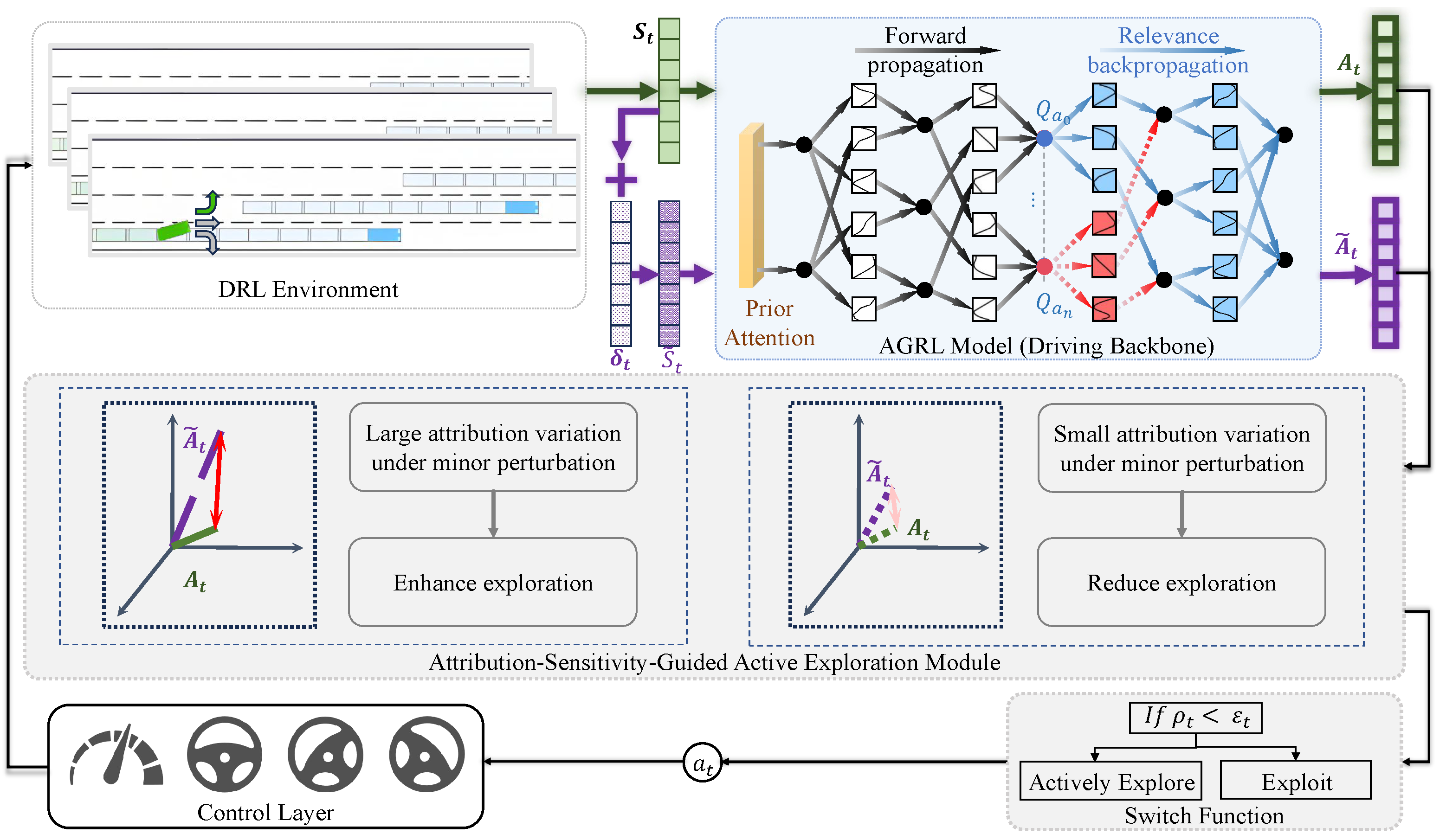
As illustrated in Figure 1, the proposed Attribution-Guided Reinforcement Learning (AGRL) framework consists of three core modules: (1) a driving decision backbone, (2) an attribution module, and (3) an attribution-sensitivity-guided exploration mechanism. Among them, the attribution module serves as the foundation of the overall framework, as it provides the feature-level attribution information required by both the prior attention mechanism and the active exploration strategy.

3.2.1. Prior-Attention-Enhanced KAN Decision Model

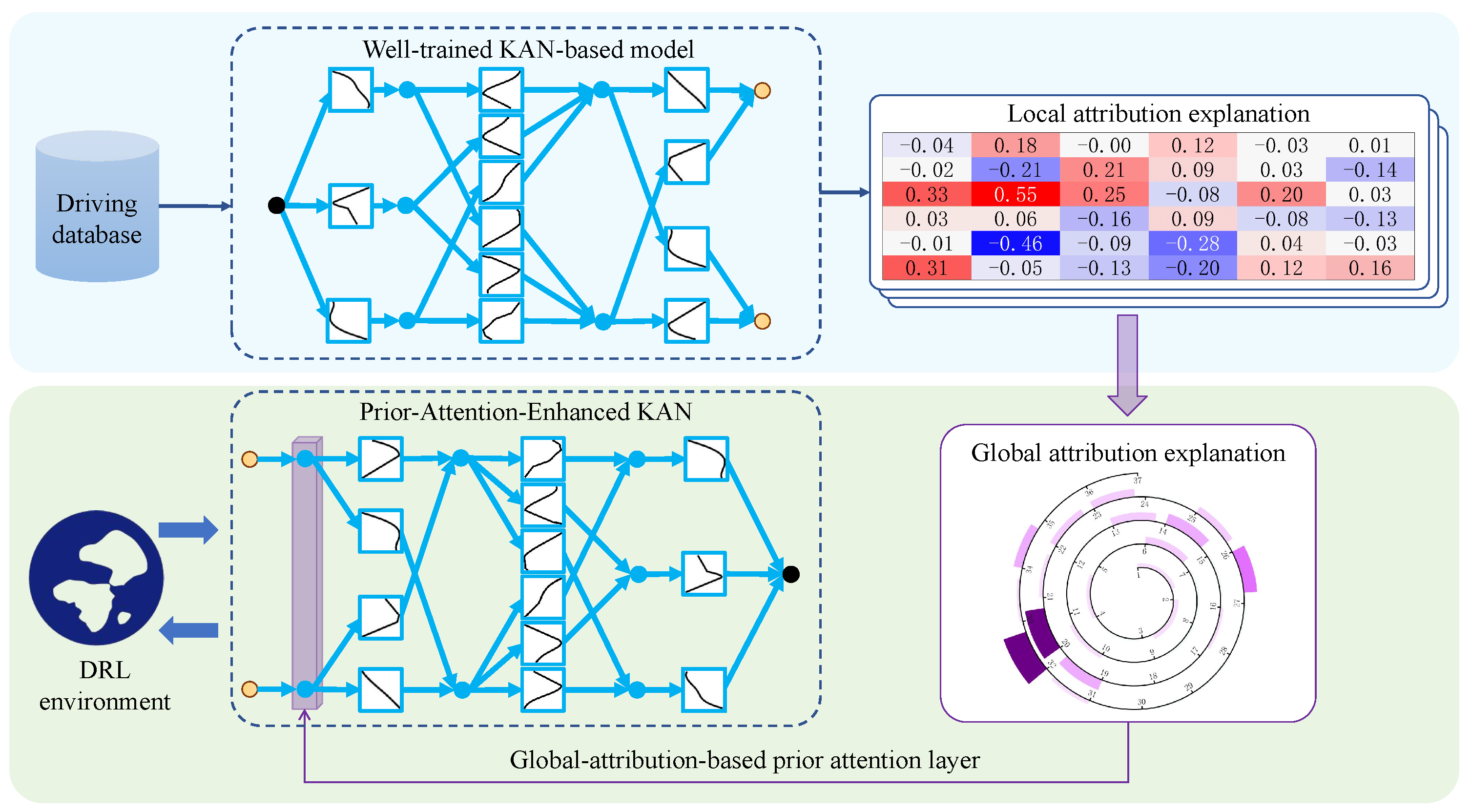
To incorporate global attribution knowledge into policy learning, we augment the original KAN-based decision model with a prior attention layer placed immediately after the input layer, as shown in Figure 2. The resulting model is referred to as a Prior-Attention-Enhanced KAN (PAE-KAN). Instead of directly using global attribution scores as fixed feature weights, the proposed model employs them to initialize a trainable prior attention gate, allowing the network to preserve attribution-based prior knowledge while retaining sufficient flexibility for task-specific adaptation.

Let $\mathbf{s}=[s_1,s_2,\dots ,s_n]$ denote the input state. The prior attention layer produces a feature-wise gate vector $\mathbf{g}=[g_1,g_2,\dots ,g_n]$, and the reweighted input is defined as

$$\widehat{\mathbf{s}}=\mathbf{g}\odot \mathbf{s},$$

(5)

where ⊙ denotes element-wise multiplication. The gate vector is parameterized as

$$\mathbf{g}=\lambda ·\sigma \left(\mathbf{z}\right),$$

(6)

where $\mathbf{z}=[z_1,z_2,\dots ,z_n]$ denotes the trainable gate logits, $\sigma (·)$ is the sigmoid function, and $\lambda$ is a scaling factor controlling the overall gate magnitude.

The reweighted input $\widehat{\mathbf{s}}$ is then fed into the subsequent decision backbone. Accordingly, the mathematical form of the proposed PAE-KAN can be expressed as

$$f\left(\mathbf{s}\right)={\displaystyle \sum _{q=1}^{2n+1}}{\mathrm{\Phi }}_q\left({\displaystyle \sum _{p=1}^n}{\varphi }_{q,p}\left({\widehat{s}}_p\right)\right),$$

(7)

where ${\widehat{s}}_p=g_p{s}_p$, ${\varphi }_{q,p}$ denotes the univariate transformation applied to the p-th reweighted input feature, and ${\mathrm{\Phi }}_q$ denotes the higher-level aggregation function. In this way, the proposed PAE-KAN explicitly integrates attribution-derived prior knowledge into the input representation, enabling the model to emphasize globally important decision-related features while suppressing less informative ones.

3.2.2. LRP-Based Real-Time Attribution Method

LRP is a post hoc interpretation method designed to identify which input variables contribute most to a model’s prediction. In our previous work, we demonstrated that combining LRP with KAN can effectively overcome the fidelity limitations encountered when applying LRP to conventional multilayer perceptrons.

In this section, we describe how attribution information can be extracted from the proposed PAE-KAN decision model. Given a scene input $S_t$, the prior attention layer first generates the reweighted state ${\widehat{S}}_t$, which is then fed into the KAN-based Q-network. For a given action a, the action-specific Q-value is denoted by $Q_a\left({\widehat{S}}_t\right)$. Attribution is used to quantify the contribution of each input feature $x_t^i$ to the predicted Q-value $Q_a\left({\widehat{S}}_t\right)$. Each action has an independent LRP propagation process. For example, in a lane-changing decision task, LRP can separately explain the predicted Q-values associated with left lane change, right lane change, and lane keeping. The LRP-based attribution process therefore consists of two main stages.

Step 1: Forward pass in PAE-KAN. For notational simplicity, let $\mathbf{X}=\widehat{\mathbf{s}}=\{{\widehat{x}}_1,{\widehat{x}}_2,\dots ,{\widehat{x}}_n\}$ denote the prior-attention-reweighted input. The forward computation of the KAN backbone is given by

$$Q\left(\mathbf{X}\right)={\displaystyle \sum _{q=1}^{2n+1}}{\varphi }_q\left({\displaystyle \sum _{p=1}^n}{\varphi }_{p,q}\left({\widehat{x}}_p\right)\right),$$

(8)

where ${\varphi }_{p,q}$ denotes the nonlinear transformation applied to the p-th reweighted input feature, and ${\varphi }_q$ represents the nonlinear transformation at the output layer. This structure can be rewritten as

$$\begin{array}{cc}\hfill Q\left({\mathbf{X}}^{\prime }\right)& ={\displaystyle \sum _{q=1}^{2n+1}}{\varphi }_q\left(X_q^{\prime }\right),\hfill \end{array}$$

(9)

$$\begin{array}{cc}\hfill X_q^{\prime }& ={\displaystyle \sum _{p=1}^n}{\varphi }_{q,p}\left({\widehat{x}}_p\right),\hfill \end{array}$$

(10)

where ${\mathbf{X}}^{\prime }=\{X_1^{\prime },X_2^{\prime },\dots ,X_{2n+1}^{\prime }\}$, and $X_q^{\prime }$ represents the activation of node q in the intermediate layer.

For deeper KAN architectures, this recursive structure is preserved. The activation value of node k in layer $l+1$ is computed as

$$a_{l+1,k}={\displaystyle \sum _{i=1}^{n_l}}{\varphi }_{l,i,k}\left(a_{l,i}\right),$$

(11)

where $a_{l,i}$ denotes the activation of node i in layer l, ${\varphi }_{l,i,k}$ is the activation function between the two nodes, and $n_l$ is the number of nodes in layer l.

Step 2: Relevance backward propagation.

Relevance is propagated from the output layer to the input layer. Based on the recursive structure in Equation (11), when node k in layer $l+1$ distributes relevance to node i in layer l, the propagated relevance is defined as

$$R_{i\leftarrow k}^{(l+1\to l)}={\displaystyle \frac{{\varphi }_{l,i,k}\left(a_{l,i}\right)}{{\sum }_i{\varphi }_{l,i,k}\left(a_{l,i}\right)}}{R}_k^{(l+1)},$$

(12)

which leads to the LRP-KAN propagation rule

$$R_i=\sum _k{\displaystyle \frac{{\varphi }_{i,k}\left(a_i\right)}{{\sum }_i{\varphi }_{i,k}\left(a_i\right)}}{R}_k.$$

(13)

Here, $R_i$ denotes the relevance score of node i in layer l, and $R_k$ denotes the relevance score of node k in layer $l+1$.

Although PAE-KAN introduces an additional prior attention layer before the KAN backbone, this layer only rescales the input representation and does not alter the subsequent relevance redistribution structure among features. Therefore, the LRP propagation rule within the KAN backbone remains unchanged, and the same relevance analysis can be directly applied to the PAE-KAN model. Moreover, the LRP-based attribution process only requires neuron activation values and simple arithmetic operations such as addition and division. This results in extremely low computational overhead, making it feasible to use attribution signals as real-time feedback during reinforcement learning.

In addition to real-time local attribution, the proposed framework further derives global attribution priors from a large number of driving scenarios. Specifically, let

$${\mathbf{r}}^{\left(m\right)}=[r_1^{\left(m\right)},r_2^{\left(m\right)},\dots ,r_d^{\left(m\right)}]$$

(14)

denote the LRP attribution vector obtained from the m-th scenario, where d is the number of input features. Since the purpose of global attribution is to characterize feature importance regardless of contribution sign, the absolute value of each attribution score is first taken. The global attribution importance of the i-th feature is then computed as

$$u_i={\displaystyle \frac{1}{M}}{\displaystyle \sum _{m=1}^M}\left|r_i^{\left(m\right)}\right|,$$

(15)

where M denotes the total number of collected scenarios.

To construct the prior attention gate, the global attribution scores are first normalized by min–max scaling:

$${\tilde{u}}_i={\displaystyle \frac{u_i-u_{\min }}{u_{\max }-u_{\min }+\epsilon }},$$

(16)

where $u_{\min }$ and $u_{\max }$ denote the minimum and maximum values in the global attribution vector, respectively, and $\epsilon$ is a small constant for numerical stability. Finally, the initial gate logits are defined using the logit transform:

$$z_i^{\left(0\right)}=\log {\displaystyle \frac{{\tilde{u}}_i}{1-{\tilde{u}}_i}},$$

(17)

which are used to initialize the trainable gate parameters $\mathbf{z}$ in Equation (6). In this way, local attribution results are aggregated into global feature-level prior knowledge, which is embedded into the PAE-KAN model as a trainable prior attention gate.

3.2.3. Attribution-Sensitivity-Guided Exploration

AGRL uses attribution variation as an action-wise sensitivity signal to guide exploration toward actions whose decision rationales are more responsive to local traffic changes. During exploratory steps, the action with the largest attribution variation is preferentially selected, as shown in Algorithm 1.

Given the current state $s_t$, the PAE-KAN-based Dueling DQN first produces the Q-values for all actions. The LRP-based attribution module subsequently generates an attribution vector for each action:

$${\mathbf{r}}_a\left(s_t\right)=[r_a^{\left(1\right)},r_a^{\left(2\right)},\dots ,r_a^{\left(d\right)}],$$

(18)

where d is the dimension of the state representation and $r_a^{\left(i\right)}$ represents the contribution of the i-th input feature to the predicted Q-value of action a.

Algorithm 1 Attribution-Sensitivity-Guided Training in AGRL

Require:  Environment $\mathcal{E}$, initialized PAE-KAN policy $Q_{\theta }$, target network $Q_{\varphi }$, replay buffer $\mathcal{D}$, exploration rate $ϵ$, perturbation coefficient $\sigma$ Ensure:  Trained AGRL policy   1: for each episode do   2:       for each decision step t do   3:             Observe current state $s_t$   4:             Compute action values $Q(s_t,a)$ for all $a\in \mathcal{A}$   5:             Compute attribution vectors ${\mathbf{r}}_a\left(s_t\right)$ for all $a\in \mathcal{A}$   6:             Generate perturbed state ${\tilde{s}}_t=s_t+{\delta }_t$, where ${\delta }_t\sim \mathcal{N}(0,{\sigma }^2{s}_t^2)$   7:             Compute attribution vectors ${\mathbf{r}}_a\left({\tilde{s}}_t\right)$ for all $a\in \mathcal{A}$   8:             for each action $a\in \mathcal{A}$ do   9:                   Compute attribution variation $D_a(s_t,{\tilde{s}}_t)={\parallel {\mathbf{r}}_a\left(s_t\right)-{\mathbf{r}}_a\left({\tilde{s}}_t\right)\parallel }_2$ 10:             end for 11:             Select action $a_t$ according to 12:             if $\mathrm{rand}\left(\right)>ϵ$ then 13:                   $a_t\leftarrow \arg {\max }_{a\in \mathcal{A}}Q(s_t,a)$ 14:             else 15:                   $a_t\leftarrow \arg {\max }_{a\in \mathcal{A}}{D}_a(s_t,{\tilde{s}}_t)$ 16:             end if 17:             Execute $a_t$ in $\mathcal{E}$ and observe reward $r_t$ and next state $s_{t+1}$ 18:             Store transition $(s_t,a_t,r_t,s_{t+1})$ in $\mathcal{D}$ 19:             Sample a mini-batch from $\mathcal{D}$ 20:             Update $Q_{\theta }$ by minimizing the temporal-difference loss 21:             Periodically update target network parameters: $\varphi \leftarrow \theta$ 22:       end for 23: end for 24: return trained AGRL policy

To evaluate attribution sensitivity, we generate a perturbed state ${\tilde{s}}_t$ from the original state $s_t$ by applying bounded stochastic perturbations in normalized feature space. For each continuous feature i, the perturbation is sampled as

$${\delta }_t^{\left(i\right)}\sim \mathcal{N}(0,{\sigma }_i^2),$$

(19)

where ${\sigma }_i$ is a feature-specific perturbation scale. The perturbed feature is then clipped to the valid normalized range,

$${\tilde{s}}_t^{\left(i\right)}=\mathrm{clip}\left(s_t^{\left(i\right)}+{\delta }_t^{\left(i\right)},-1,1\right).$$

(20)

Binary features are kept unchanged. This feature-aware perturbation scheme ensures that the perturbed state remains bounded and semantically meaningful, while preventing out-of-range values and unrealistic observations. The perturbation scales used for the continuous features are listed in

Table 1. Standard deviations of Gaussian perturbations in the normalized feature space.

Feature Type	Variable	Standard Deviation ${\mathit{\sigma }}_{\mathit{i}}$
Binary/discrete	presence	0
Continuous	x	0.03
Continuous	y	0.03
Continuous	$v_x$	0.02
Continuous	$v_y$	0.02
Continuous	$a_x$	0.01

.

The attribution variation in action a is quantified by the Euclidean distance between the attribution vectors before and after perturbation:

$$D_a(s_t,{\tilde{s}}_t)={∥{\mathbf{r}}_a\left(s_t\right)-{\mathbf{r}}_a\left({\tilde{s}}_t\right)∥}_2.$$

(21)

Here, $D_a$ measures the sensitivity of the attribution pattern of action a to input perturbation.

During training, the action selection mechanism follows an attribution-guided $ϵ$-exploration strategy. Specifically, with probability $1-ϵ$, the agent selects the greedy action according to the predicted Q-values:

$$a_t^{\mathrm{greedy}}=\arg \underset{a\in \mathcal{A}}{\max }Q({\widehat{s}}_t,a).$$

(22)

With probability $ϵ$, instead of selecting a random action as in conventional $ϵ$-greedy exploration, the agent selects the action with the largest attribution variation:

$$a_t^{\mathrm{explore}}=\arg \underset{a\in \mathcal{A}}{\max }{D}_a(s_t,{\tilde{s}}_t).$$

(23)

Accordingly, the overall action selection rule can be expressed as

$$a_t=\left\{\begin{array}{cc}\arg {\max }_{a\in \mathcal{A}}Q({\widehat{s}}_t,a),\hfill & \mathrm{with}\mathrm{probability}1-ϵ,\hfill \\ \arg {\max }_{a\in \mathcal{A}}{D}_a(s_t,{\tilde{s}}_t),\hfill & \mathrm{with}\mathrm{probability}ϵ.\hfill \end{array}\right.$$

(24)

This design differs from random exploration. Instead of assigning exploration opportunities uniformly across actions, the proposed strategy prioritizes actions whose attribution patterns show stronger responses to small state perturbations. In other words, exploration is directed toward actions whose internal decision rationales are more locally sensitive to the current traffic situation, enabling the agent to collect more targeted training experiences than purely random exploration.

4. Implementation

This section describes the simulation environments and MDP formulation adopted for training and evaluation. Three representative driving tasks are considered, namely highway lane changing, main-road yielding, and on-ramp merging.

4.1. Scenario Modeling

All experiments are conducted in the Highway-Env simulator [34], which has been widely used in the evaluation of DRL decision-making methods for autonomous driving [35]. To comprehensively assess the proposed framework, three scenarios with increasing behavioral complexity are designed: a highway lane-change scenario, a main-road yielding scenario, and an on-ramp merging scenario.

As shown in Figure 3, the highway lane-change scenario considers an ego vehicle driving on a four-lane highway, where the agent is required to make discrete lane-selection decisions while balancing efficiency and safety. Each training run in this scenario contains 300 episodes, and each episode lasts for at most 200 time steps. Since one step corresponds to one second of simulation time, the maximum episode duration is 200 s. The longitudinal motion of all vehicles is governed by the Intelligent Driver Model (IDM) [36], while the lane-changing behavior of surrounding vehicles follows the MOBIL model [37]. The initial spacing between vehicles is 30 m, corresponding to approximately 133 vehicles/km.

The main-road yielding scenario is more challenging because the ego vehicle travels on the main road while interacting with a ramp vehicle that may merge with limited situational awareness. The ego vehicle is initialized near a location where conflict with the incoming ramp vehicle is likely. In addition, a visual obstruction is introduced, as indicated by the brown blocked area in Figure 3, preventing the ramp vehicle from observing the main-road traffic before reaching the acceleration lane. As a result, the ramp vehicle may initiate a merge without complete knowledge of surrounding traffic. In contrast, the ego vehicle is able to observe the ramp vehicle and must make both longitudinal and lateral decisions to avoid potential conflicts. In this scenario, the ramp length is 80 m, followed by an 80 m acceleration lane. After merging, the vehicle is required to travel safely for another 150 m. Surrounding vehicles are generated randomly with an average initial longitudinal spacing of 40 m, leaving a feasible but nontrivial merging opportunity.

Among the three scenarios, on-ramp merging poses the highest level of difficulty. In this task, the ego vehicle starts from the ramp and must identify an appropriate gap before merging safely into the main-road traffic. Excessively aggressive behavior is penalized because it may violate safe spacing requirements, whereas overly conservative behavior may cause merge failure. The ramp length in this scenario is 80 m, followed by a 150 m acceleration lane. After merging, the ego vehicle must continue safely for an additional 150 m on the main road. For both the on-ramp merging and main-road yielding scenarios, each training run consists of 2000 episodes. Vehicles are generated randomly with an average initial longitudinal spacing of 25 m, which creates denser traffic interactions and increases the difficulty of successful merging.

In all scenarios, inappropriate decisions may lead to hazardous interactions and, in severe cases, collisions. An episode is regarded as successful if the ego vehicle completes the task without collision; otherwise, the episode is recorded as a failure and the environment is reset. Based on this setup, the driving task is formulated as an MDP by defining the observation space, action space, and reward function.

4.2. Observation and Action Space

The agent is assumed to perceive a local traffic region surrounding the ego vehicle. In both the highway lane-change and on-ramp merging scenarios, the observation range covers the current lane and its two adjacent lanes. Specifically, in the current lane, the agent observes the ego vehicle itself together with the nearest leading vehicle. In each adjacent lane, both the nearest leading and trailing vehicles are included in the observation. In the main-road yielding scenario, besides six vehicles on the main road, the agent additionally observes the nearest vehicle on the ramp.

Each vehicle is represented by a state vector $S_i$ containing its relative kinematic information. For the ego vehicle, the state representation is defined as

$$S_1=(p_1,\Delta x,\Delta y,v_{x_1},v_{y_1},a_1),$$

(25)

where $\Delta x$ and $\Delta y$ denote the distances from the ego vehicle to the left and right road boundaries, respectively. The remaining terms $v_{x_1}$, $v_{y_1}$, and $a_1$ represent the longitudinal velocity, lateral velocity, and longitudinal acceleration of the ego vehicle.

For surrounding vehicles, the state vector is written as

$$S_i=(p_i,\Delta x_i,\Delta y_i,v_{x_i},v_{y_i},a_i),$$

(26)

where $\Delta x_i$ and $\Delta y_i$ denote the relative longitudinal and lateral positions with respect to the ego vehicle, and $v_{x_i}$, $v_{y_i}$, and $a_i$ are the corresponding kinematic variables. If a surrounding vehicle is outside the perception range, its indicator $p_i$ is set to zero. Under this definition, the observation dimension is 36 for the highway lane-change and on-ramp merging scenarios, and 42 for the main-road yielding scenario.

4.3. Action Space

The highway lane-change task is formulated as a discrete decision problem with three candidate actions:

$$a_t=(a_0,a_1,a_2),$$

where $a_0$, $a_1$, and $a_2$ denote left lane change, lane keeping, and right lane change, respectively.

For the main-road yielding and on-ramp merging tasks, the action set is extended to include longitudinal control, resulting in a five-dimensional discrete action space:

$$a_t=(a_0,a_1,a_2,a_3,a_4),$$

where $a_0$, $a_1$, and $a_2$ retain the same meanings as above, while $a_3$ and $a_4$ correspond to acceleration and deceleration, respectively.

4.4. Reward Function

The reward function is designed to jointly account for efficiency, safety, comfort, and energy-related objectives, so that the learned policy better matches practical autonomous driving requirements. The overall reward at time step t is defined as

$$r_t=R_{\mathrm{speed}}-C_{\mathrm{comfort}}-C_{\mathrm{distance}}-C_{\mathrm{collision}}-C_{\mathrm{fuel}}-C_{\mathrm{merge}}.$$

(27)

The individual terms are defined as follows.

(1)

Speed reward. To encourage efficient travel, the speed reward is defined as

$$R_{\mathrm{speed}}={\alpha }_1·{\displaystyle \frac{v_t-v_{\min }}{v_{\max }-v_{\min }}},$$

(28)

where $v_t$ is the current speed of the ego vehicle, and $v_{\min }$ and $v_{\max }$ are the lower and upper bounds of the desired speed interval.

(2)

Comfort cost. To discourage excessive longitudinal acceleration and unnecessary lane changes, the comfort cost is given by

$$C_{\mathrm{comfort}}={\alpha }_2\left|{\mathrm{acc}}_t\right|+{\alpha }_3{\delta }_{\mathrm{lc}},$$

(29)

where ${\mathrm{acc}}_t$ denotes the longitudinal acceleration and ${\delta }_{\mathrm{lc}}$ is a binary indicator for lane-change execution.

(3)

Safe-distance cost. To penalize unsafe following behavior and near-collision situations, the safe-distance cost is defined as

$$C_{\mathrm{distance}}=\left\{\begin{array}{cc}{\alpha }_5,\hfill & \mathrm{if}0<d_{\mathrm{safe}}<5\mathrm{m},\hfill \\ {\alpha }_5\left(1-{\displaystyle \frac{d_{\mathrm{safe}}-5}{5}}\right),\hfill & \mathrm{if}5\mathrm{m}\le d_{\mathrm{safe}}<10\mathrm{m},\hfill \\ 0,\hfill & \mathrm{otherwise},\hfill \end{array}\right.$$

(30)

where $d_{\mathrm{safe}}$ represents the distance to the nearest leading vehicle in the current lane, and ${\alpha }_5$ controls the penalty strength.

(4)

Collision penalty. To explicitly discourage unsafe behaviors that lead to crashes, the collision penalty is defined as

$$C_{\mathrm{collision}}=\left\{\begin{array}{cc}1,\hfill & \mathrm{if}\mathrm{a}\mathrm{collision}\mathrm{occurs},\hfill \\ 0,\hfill & \mathrm{otherwise}.\hfill \end{array}\right.$$

(31)

(5)

Merging speed penalty. For the main-road yielding scenario, an additional penalty is imposed when the merging vehicle moves too slowly, encouraging the ego vehicle to create sufficient space for safe merging:

$$C_{\mathrm{merge}}={\alpha }_6·{\displaystyle \frac{v_{\max }-v_t^m}{v_{\max }}},$$

(32)

where $v_t^m$ denotes the instantaneous speed of the merging vehicle and $v_{\max }$ is the upper speed bound.

5. Experimental Results

In this section, the proposed AGRL framework is evaluated through comprehensive empirical studies. First, AGRL is compared with representative baseline methods in three autonomous driving decision-making scenarios, namely highway lane changing, main-road yielding, and on-ramp merging. Then, two groups of ablation studies are conducted in the highway lane-change scenario. The first group separately verifies the effectiveness of the global-attribution-based prior attention mechanism and the attribution-sensitivity-guided exploration module. The second group compares different attribution-change metrics as exploration signals to justify the use of Euclidean attribution variation in AGRL. Finally, an interpretability analysis is provided to illustrate how the proposed attribution-sensitivity signal reflects action-wise local responses to perturbations.

5.1. Baselines

To evaluate the effectiveness of the proposed AGRL framework, comprehensive comparisons are conducted against several representative baseline methods. The selected baselines are divided into two categories: standard value-based reinforcement learning methods and active-exploration-based methods.

• Standard value-based RL baselines: Deep Q-Network (DQN) [38], Double DQN (DDQN) [39], and Dueling DQN (DuDQN) [33]. These methods are adopted as conventional value-based baselines that rely on standard random exploration strategies.
• Interpretable value-based RL baseline: KAN-IDRL is included to distinguish the contribution of the KAN-based interpretable policy representation from that of the proposed attribution-guided exploration mechanism. Similar to the above value-based baselines, KAN-IDRL also relies on random exploration.
• Active-exploration baselines: Random Network Distillation (RND) is included as a representative intrinsic-motivation-based exploration method, Intrinsic Curiosity Module (ICM) [13] is added as a representative curiosity-driven exploration method, while SimHash [40] is employed as a representative count-based exploration method. For a fair comparison, RND, ICM, and SimHash are all re-implemented on the same Dueling DQN backbone, with only the exploration mechanism changed. These three methods are selected as baselines to compare the proposed AGRL framework against classical active-exploration strategies.

All compared methods are implemented within a value-based reinforcement learning framework. To ensure a fair comparison, the same network training settings and optimization hyperparameters are used across all methods within each scenario, as summarized in

Table 2. Hyperparameters for different driving scenarios.

Parameters	Highway Lane-Change	Main-Road Yielding	On-Ramp Merging
Total Episodes	300	1000	2000
Discount Factor	0.8	0.8	0.95
Soft Update Rate	0.005	0.005	0.005
Exploration Decay Rate	$5\times {10}^{-4}$	$5\times {10}^{-5}$	$5\times {10}^{-5}$
Replay Buffer Capacity	$1\times {10}^6$	$1\times {10}^6$	$1\times {10}^6$
Batch Size	256	256	256

. In addition, each algorithm is trained with five different random seeds to improve statistical reliability.

5.2. Evaluation Metrics

During training, the learning process in the highway lane-change scenario is evaluated using five metrics: average cumulative reward, success rate, average speed, comfort cost, and safety cost. For the main-road yielding and on-ramp merging scenarios, comfort cost is not considered, while an additional metric, namely merging speed cost, is introduced. Among these metrics, comfort cost, safety cost, and merging speed cost are computed according to Equation (29), Equation (30), and Equation (32), respectively. The cumulative reward is defined as the total reward accumulated over an episode, where the reward at each time step is computed according to Equation (27). As a comprehensive performance indicator, cumulative reward reflects the overall trade-off among efficiency, safety, comfort, and task-related objectives. The success rate is defined as the proportion of episodes in which the autonomous agent completes the driving task without collision or failure. Average speed is used to characterize driving efficiency more directly.

In addition to the above driving-performance metrics, we further evaluate training-stage safety and convergence efficiency. Training-stage safety is measured by the number of collisions during training, where a collision refers to the ego vehicle colliding with surrounding vehicles or road boundaries. Convergence efficiency is quantified by the number of episodes required to reach a predefined reward threshold. Let $R_e$ denote the episodic return at episode e. We first compute the moving-average reward with a window size of W:

$${\overline{R}}_e={\displaystyle \frac{1}{W}}{\displaystyle \sum _{i=e-W+1}^e}{R}_i.$$

(33)

The number of episodes required to reach the reward threshold is then defined as:

$$E_{\mathrm{reward}}=\min \{e\mid {\overline{R}}_e\ge R_{\mathrm{th}}\},$$

(34)

where $R_{\mathrm{th}}$ denotes the predefined reward threshold. This metric is computed independently for each random seed.

The moving-average window size W, and reward threshold $R_{\mathrm{th}}$ used for convergence evaluation are summarized in

Table 3. Settings for convergence-threshold evaluation in different scenarios.

Scenario	Window Size W	Reward Threshold ${\mathit{R}}_{\mathbf{th}}$
Highway lane-change	30	24.0
Main-road yielding	100	9.0
On-ramp merging	200	7.5

. The threshold in each scenario is selected as approximately 90% of the final moving-average reward achieved by AGRL, so that the convergence metric reflects the episode at which each method reaches a near-converged performance level.

5.3. Policy Evaluation

5.3.1. Decision Model Training

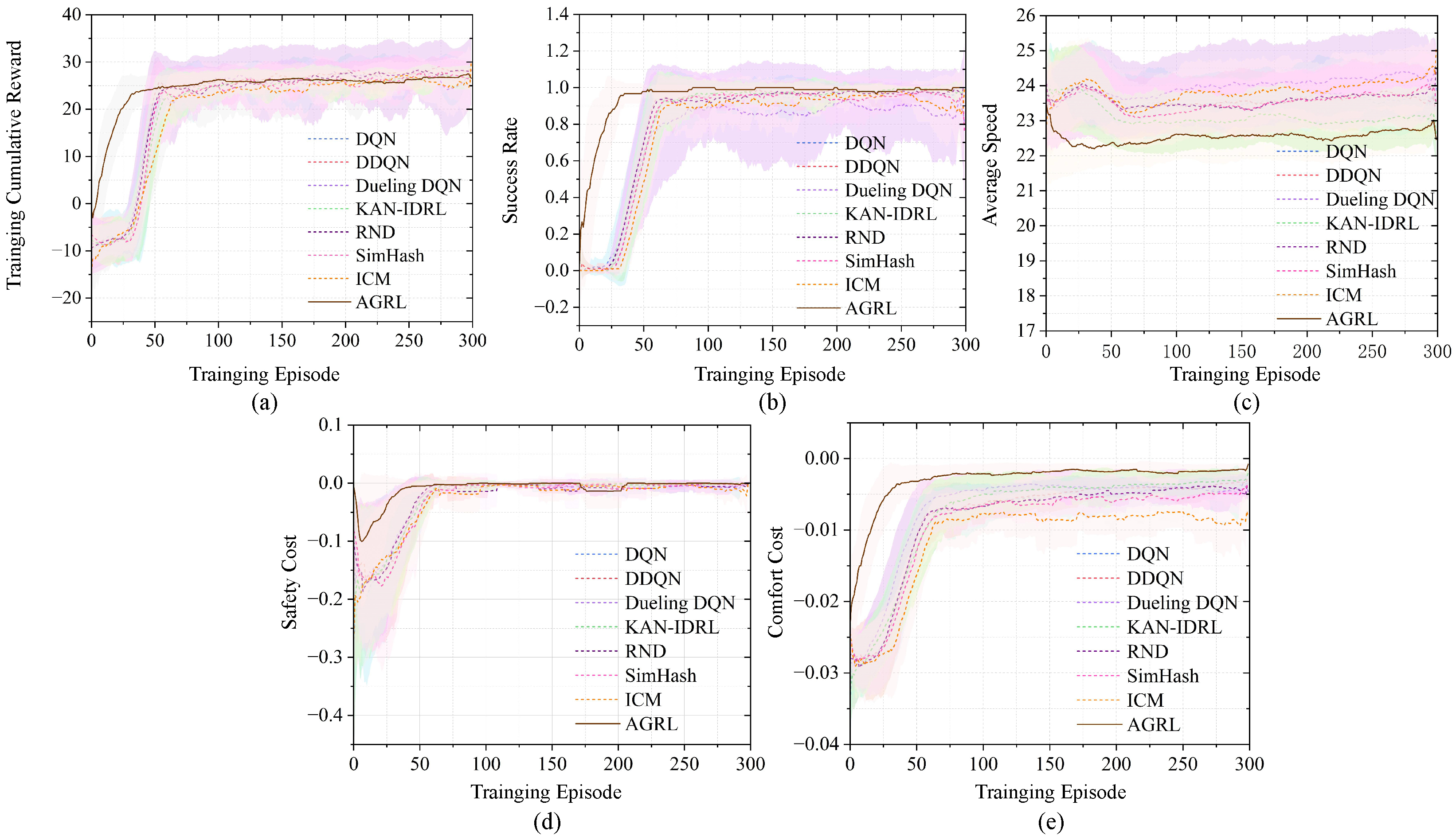
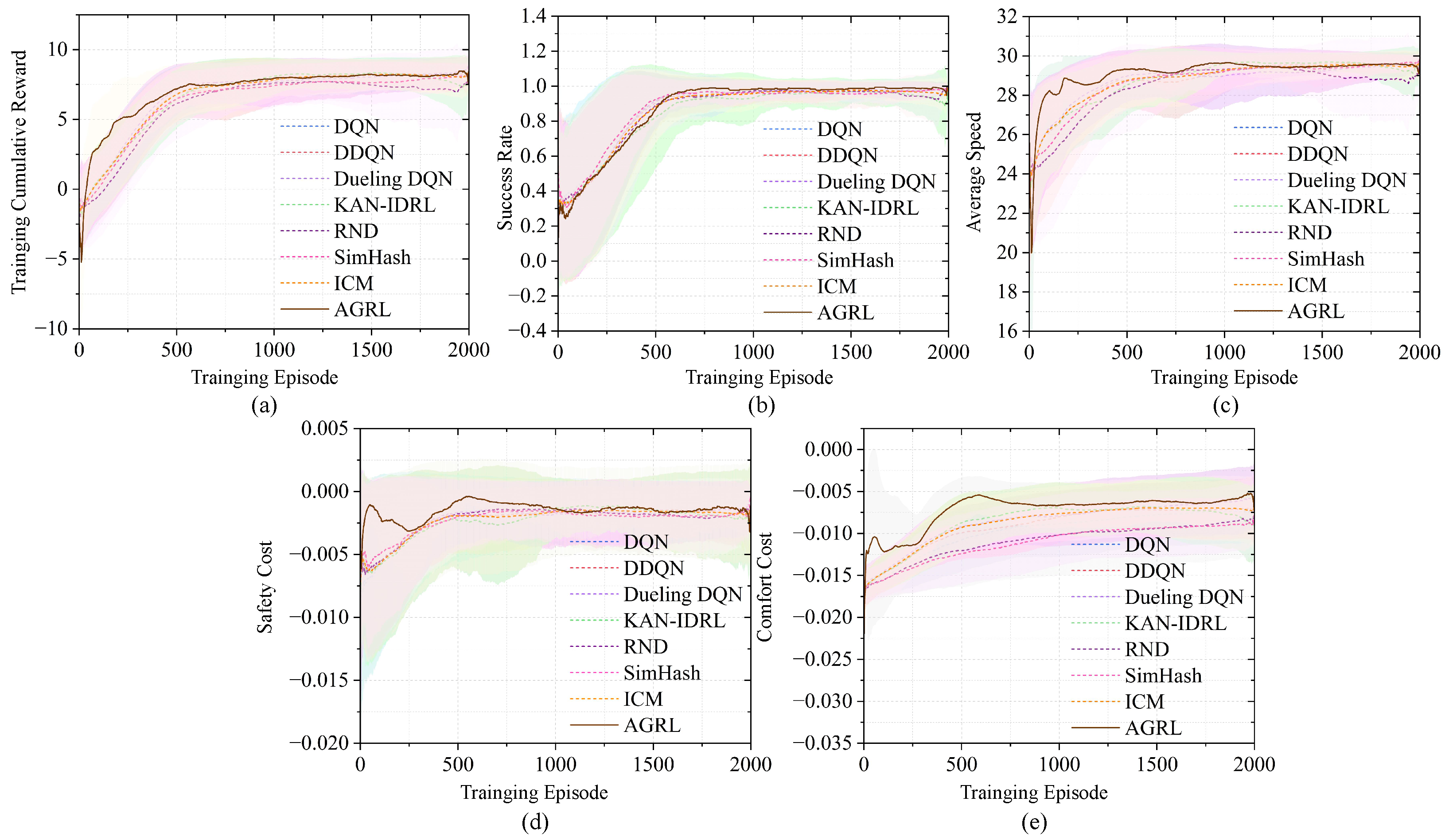
Figure 4 illustrates the learning curves in the highway lane-change scenario. Compared with all baseline methods, AGRL exhibits substantially faster convergence in terms of cumulative reward, success rate, safety cost, and comfort cost. In particular, the proposed method reaches a stable and favorable performance level considerably earlier than the baseline methods. By contrast, AGRL yields a relatively lower average speed, indicating that the learned policy tends to adopt a more conservative driving style in exchange for improved safety and higher overall return.

It is also observed that RND, SimHash, and ICM achieve performance close to that of conventional value-based baselines such as DQN, DDQN, and DuDQN. One important reason is that these methods rely on external novelty estimation mechanisms, such as state prediction or state counting, to guide exploration. However, the driving environments considered in this work exhibit strong uncertainty. Surrounding vehicles change lanes autonomously and also respond to the behavior of the ego vehicle, making the environment highly dynamic and partially non-stationary. Under such conditions, predicting future states or constructing reliable novelty estimates becomes inherently difficult. In fact, modeling the environment well enough to support effective exploration is nearly as challenging as learning the driving policy itself. As a result, the additional exploration signals provided by RND, SimHash, and ICM become less informative, which limits their advantage over conventional random-exploration baselines. In contrast, the proposed AGRL framework does not rely on an auxiliary model to predict environmental novelty. Instead, it depends only on the internal attribution signals of the decision model itself, making the exploration signal more directly coupled to the policy’s local decision response and therefore more effective in highly complex driving environments.

Table 4. Training-stage collision count and convergence episodes in the highway lane-change scenario. Bold values indicate the best performance among all compared methods.

Method	Training Collisions	Convergence Episodes
DQN	$57.6\pm 5.18$	$77.0\pm 8.15$
DDQN	$75.8\pm 4.27$	$80.8\pm 14.4$
Dueling DQN	$63.5\pm 6.74$	$84.2\pm 11.4$
KAN-IDRL	$39.6\pm 8.45$	$78.2\pm 19.7$
RND	$53.6\pm 4.74$	$78.8\pm 13.4$
SimHash	$58.3\pm 4.72$	$90.8\pm 17.25$
ICM	$67.7\pm 6.35$	$95.9\pm 14.2$
AGRL	$\mathbf{23.4}\pm \mathbf{7.57}$	$\mathbf{65.8}\pm \mathbf{14.5}$

summarizes the total number of training-stage collisions and the convergence episodes in the highway lane-change scenario. Compared with the baseline methods, AGRL requires fewer episodes to reach convergence, with an average convergence episode of $65.8$, while the other methods require between $77.0$ and $90.8$ episodes. Moreover, AGRL substantially reduces the number of collisions during training. Specifically, AGRL records only $23.4\pm 7.57$ collisions, which is substantially lower than all baseline methods. Therefore, in the highway lane-change scenario, AGRL provides advantages in both learning efficiency and training-stage safety.

In addition to convergence efficiency, we further analyze the computational overhead of different methods in the highway lane-change scenario. All simulation experiments were conducted on a computer equipped with an Intel i9-10900K CPU, an NVIDIA GeForce RTX 3090 GPU, and 32 GB of RAM. The comparison includes the number of trainable parameters, runtime per training step, total training time, and single-step inference latency during deployment, as reported in

Table 5. Computational overhead comparison in the highway lane-change scenario.

Method	Trainable Params.	Runtime/Step	Total Training Time	Inference Latency
Dueling DQN	76,292	0.0600	3099.96 s	0.0589
KAN-IDRL	2400	0.0754	4086.24 s	0.0625
RND	184,452	0.0616	3148.73 s	0.0587
SimHash	76,292	0.0606	3175.52 s	0.0589
ICM	251,911	0.0620	3130.67 s	0.0588
AGRL	2436	0.0830	4759.39 s	0.0624

.

In terms of trainable parameters, AGRL remains lightweight. The KAN-IDRL backbone contains only 2400 trainable parameters, and the prior-attention layer introduced in AGRL adds only a small number of additional parameters. As a result, AGRL has 2436 trainable parameters, which is substantially fewer than Dueling DQN, RND, and ICM.

However, AGRL introduces additional computational cost during training. Its runtime per training step and total training time are higher than those of the DQN-based baselines. This overhead mainly comes from two sources: the spline-based computation in KAN and the additional forward and attribution-computation operations required to obtain the attribution-sensitivity signal. The spline-based computation is inherent to the KAN-based policy and remains during deployment, whereas the exploration-specific operations are mainly incurred during training. During deployment, the additional perturbed-state forward pass and attribution computation can be disabled, resulting in an inference latency close to that of KAN-IDRL.

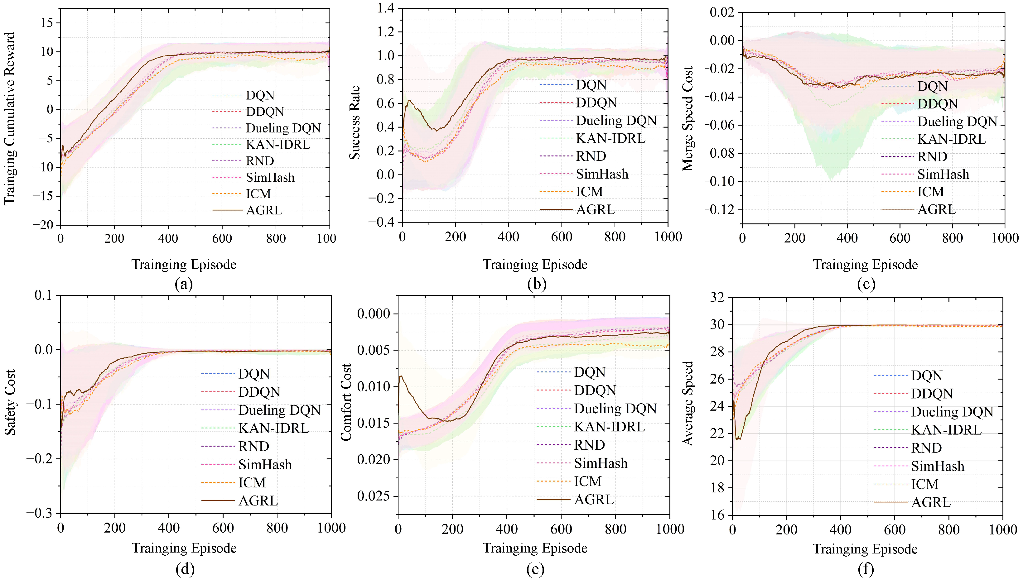
Figure 5 presents the learning curves in the main-road yielding scenario. AGRL again demonstrates a clear advantage in convergence speed over the baseline methods. Although its cumulative reward is lower than that of some baselines during the early training stage, its success rate is higher at the same time, suggesting that the learned policy initially favors safer and more conservative actions. As training proceeds, the policy gradually learns to balance safety and efficiency more effectively, which is reflected in the rapid improvement of both cumulative reward and average speed. Similar to the observations in the highway lane-change scenario, the performance of RND, SimHash, and ICM remains close to that of the conventional value-based baselines, indicating that their exploration advantage is limited in the current driving task.

Table 6. Training-stage collision count and convergence episodes in the main-road yielding scenario. Bold values indicate the best performance among all compared methods.

Method	Training Collisions	Convergence Episodes
DQN	$253.2\pm 16.6$	$471.4\pm 14.7$
DDQN	$239.2\pm 19.3$	$447.4\pm 13.9$
Dueling DQN	$245.6\pm 21.8$	$459.8\pm 16.5$
KAN-IDRL	$221.4\pm 24.6$	$438.6\pm 18.7$
RND	$248.2\pm 15.7$	$457.6\pm 8.6$
SimHash	$250.8\pm 18.7$	$463.6\pm 11.0$
ICM	$281.0\pm 42.3$	$453.0\pm 13.5$
AGRL	$\mathbf{185.4}\pm \mathbf{34.1}$	$\mathbf{415.2}\pm \mathbf{21.4}$

reports the training-stage collision count and convergence episodes in the main-road yielding scenario. AGRL achieves the fastest convergence, requiring only $415.2$ episodes on average, whereas the baseline methods require between $438.6$ and 471.4 episodes. AGRL also records the fewest training-stage collisions, with 185.4 ± 34.1 collisions, which is substantially lower than all baseline methods.

Figure 6 shows the learning curves in the on-ramp merging scenario. This scenario is more challenging because purely conservative behavior cannot successfully complete the task; if the ego vehicle fails to merge within the designated road segment, the episode is terminated as a failure. Despite this increased complexity, AGRL still achieves faster convergence than the baseline methods. This result indicates that the proposed framework is able to guide the agent more efficiently toward effective decision policies even in tasks that require a delicate balance between safety and assertiveness. The superior training performance in this scenario further demonstrates the robustness and adaptability of AGRL under more demanding decision-making conditions.

Table 7. Training-stage collision count and convergence episodes in the on-ramp merging scenario. Bold values indicate the best performance among all compared methods.

Method	Training Collisions	Convergence Episodes
DQN	$238.6\pm 25.6$	$743.4\pm 165.4$
DDQN	$251.6\pm 9.4$	$773.2\pm 229.1$
Dueling DQN	$241.0\pm 23.0$	$673.8\pm 109.7$
KAN-IDRL	$\mathbf{232.8}\pm \mathbf{27.4}$	$652.6\pm 96.5$
RND	$249.4\pm 22.1$	$721.6\pm 138.2$
SimHash	$255.2\pm 24.7$	$734.8\pm 151.6$
ICM	$263.8\pm 31.5$	$706.4\pm 127.3$
AGRL	$246.0\pm 20.8$	$\mathbf{617.3}\pm \mathbf{53.0}$

reports the training-stage collision count and convergence episodes in the on-ramp merging scenario, AGRL achieves the fastest convergence in the on-ramp merging scenario, requiring only $617.3$ episodes on average, while the baseline methods require between $652.6$ and $773.2$ episodes. For training-stage collisions, AGRL obtains $246.0\pm 20.8$, which is comparable to most baseline methods and lower than DDQN, RND, SimHash, and ICM. Although it does not produce the lowest collision count, AGRL achieves a clear convergence advantage while maintaining a comparable level of training safety in this challenging merging task.

5.3.2. Decision Model Testing

This subsection presents a quantitative comparison of all methods across the three driving scenarios.

As shown in

Table 8. Performance comparison of all algorithms in the highway lane-change scenario. Bold values indicate the best performance among all compared methods.

Method	Avg. Cumulative Reward	Success Rate (%)	Avg. Speed (m/s)	Safety Cost (×${10}^{-3}$)	Comfort Cost (×${10}^{-3}$)
DQN	26.04 ± 1.84	96.35 ± 2.54	23.89 ± 1.12	−8.5 ± 8.21	−6.1 ± 0.81
DDQN	26.13 ± 1.70	95.11 ± 2.89	23.84 ± 1.08	−7.4 ± 7.68	−5.3 ± 0.57
Dueling DQN	25.86 ± 1.76	95.72 ± 2.67	24.30 ± 1.15	−9.3 ± 8.46	−4.6 ± 0.74
KAN	25.49 ± 1.58	95.67 ± 2.31	23.40 ± 0.96	−7.8 ± 7.24	−4.3 ± 0.62
RND	26.25 ± 1.69	95.34 ± 2.76	23.76 ± 1.04	−9.6 ± 8.73	−5.4 ± 0.79
SimHash	25.59 ± 1.63	95.76 ± 2.48	23.84 ± 1.01	−2.4 ± 2.16	−6.3 ± 0.86
ICM	26.18 ± 1.72	95.58 ± 2.62	23.91 ± 1.06	−8.8 ± 8.05	−5.7 ± 0.77
AGRL	26.57 ± 1.21	98.45 ± 2.18	23.21 ± 0.88	−2.3 ± 1.74	−2.7 ± 0.61

, all methods perform well in the highway lane-change scenario, with success rates above 95%. Among them, AGRL achieves the highest average cumulative reward of 26.57, the highest success rate of 98.45%, and the lowest safety and comfort costs, i.e., $-0.0023$ and $-0.0027$, respectively. Although AGRL yields a slightly lower average speed than the Dueling DQN baseline, its success rate is 2.73% higher. These results indicate that AGRL achieves the best overall driving performance in this scenario and provides a more favorable balance between safety and efficiency.

In the more complex main-road yielding scenario, AGRL outperforms all baseline methods in terms of cumulative reward, success rate, and average speed. As shown in

Table 9. Performance comparison of all algorithms in the main-road yielding scenario. Bold values indicate the best performance among all compared methods.

Method	Avg. Cumulative Reward	Success Rate (%)	Avg. Speed (m/s)	Merging Speed Cost (×${10}^{-3}$)	Safety Cost (×${10}^{-3}$)
DQN	10.07 ± 0.46	96.45 ± 2.18	29.95 ± 0.42	−1.58 ± 0.61	−0.68 ± 0.29
DDQN	10.03 ± 0.51	95.40 ± 2.47	29.92 ± 0.45	−2.01 ± 0.74	−0.79 ± 0.33
Dueling DQN	10.29 ± 0.43	95.53 ± 2.36	29.81 ± 0.48	−1.51 ± 0.58	−0.84 ± 0.36
KAN	9.649 ± 0.57	95.11 ± 2.69	29.03 ± 0.63	−2.29 ± 0.82	−1.24 ± 0.45
RND	10.11 ± 0.49	96.24 ± 2.21	29.94 ± 0.44	−2.07 ± 0.76	−0.87 ± 0.37
SimHash	10.19 ± 0.47	95.97 ± 2.33	29.75 ± 0.50	−1.89 ± 0.69	−0.90 ± 0.39
ICM	10.16 ± 0.48	96.08 ± 2.29	29.88 ± 0.46	−1.96 ± 0.72	−0.86 ± 0.35
AGRL	10.32 ± 0.31	97.67 ± 1.42	29.96 ± 0.28	−2.09 ± 0.64	−0.69 ± 0.27

, AGRL attains a success rate of 97.67% while simultaneously achieving the highest average speed of 29.96 m/s and the highest cumulative reward of 10.32. These results suggest that AGRL is able to promote more effective learning of complex yielding behaviors, enabling the agent to maintain both traffic efficiency and collision avoidance performance under interactive driving conditions.

In the most challenging on-ramp merging scenario, which requires real-time gap selection and fine-grained speed control, AGRL also demonstrates strong performance. As shown in

Table 10. Performance comparison of all algorithms in the on-ramp merging scenario. Bold values indicate the best performance among all compared methods.

Method	Avg. Cumulative Reward	Success Rate (%)	Avg. Speed (m/s)	Safety Cost (×${10}^{-3}$)	Comfort Cost (×${10}^{-3}$)
DQN	8.32 ± 0.54	97.13 ± 1.96	29.71 ± 0.39	−2.15 ± 0.82	−9.62 ± 1.74
DDQN	8.51 ± 0.49	96.35 ± 2.21	29.84 ± 0.35	−1.65 ± 0.71	−5.84 ± 1.21
Dueling DQN	8.12 ± 0.61	93.51 ± 2.84	29.74 ± 0.42	−1.86 ± 0.76	−8.59 ± 1.58
KAN	8.16 ± 0.58	96.87 ± 2.05	29.65 ± 0.44	−2.31 ± 0.89	−6.48 ± 1.36
RND	8.04 ± 0.63	97.05 ± 1.98	29.55 ± 0.47	−2.19 ± 0.85	−6.74 ± 1.42
SimHash	8.42 ± 0.52	96.75 ± 2.13	29.21 ± 0.51	−1.98 ± 0.79	−7.51 ± 1.49
ICM	8.39 ± 0.55	96.92 ± 2.07	29.68 ± 0.43	−1.91 ± 0.77	−6.21 ± 1.30
AGRL	8.64 ± 0.34	98.32 ± 1.17	29.57 ± 0.31	−1.24 ± 0.52	−4.34 ± 0.96

, AGRL achieves the highest success rate of 98.32%, the highest cumulative reward of 8.64, and the lowest safety and comfort costs. Although its average speed is slightly lower than that of DDQN, its success rate remains 1.97% higher. This result indicates that AGRL is better able to balance aggressiveness and safety in difficult merging tasks, thereby improving the overall quality of the learned policy.

Overall, AGRL achieves the strongest driving performance across all scenarios, consistently obtaining the highest average cumulative reward and the highest success rate.

5.4. Ablation Study

To further analyze the contribution of different components in AGRL, we conduct two groups of ablation studies. The first group evaluates the effectiveness of the main algorithmic components, including the prior-attention mechanism and the attribution-sensitivity-guided exploration module. The second group compares different attribution-change metrics as exploration signals to verify the choice of Euclidean attribution variation.

5.4.1. Component Ablation

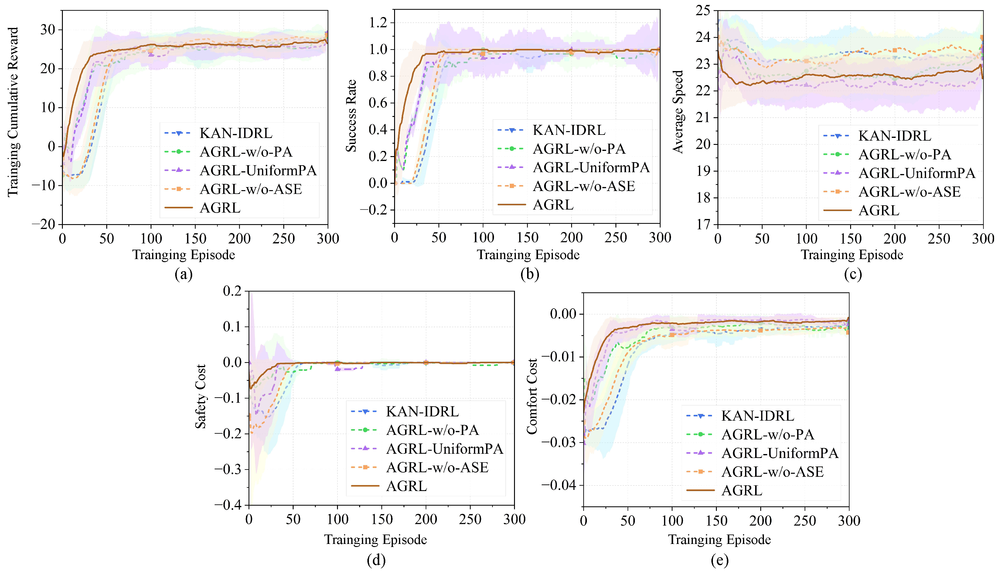
This experiment evaluates the individual contributions of the global-attribution-based prior attention mechanism and the attribution-sensitivity-guided exploration module. Specifically, we compare AGRL with four ablated variants: KAN-IDRL, AGRL-w/o-PA, AGRL-UniformPA, and AGRL-w/o-ASE. KAN-IDRL denotes the backbone model without prior attention or attribution-sensitivity-guided exploration. AGRL-w/o-PA removes the prior-attention module while retaining attribution-sensitivity-guided exploration. AGRL-UniformPA keeps the trainable prior-attention gate but initializes all attention coefficients to 1, so that no attribution-derived feature preference is introduced at initialization. AGRL-w/o-ASE retains the attribution-derived prior attention but removes the attribution-sensitivity-guided exploration module and uses random exploration instead.

As shown in Figure 7, the variants without the attribution-sensitivity-guided exploration module, including KAN-IDRL and AGRL-w/o-ASE, show clear performance degradation in cumulative reward, success rate, and convergence speed. This indicates that the attribution-sensitivity-guided exploration strategy plays an important role in improving exploration efficiency. AGRL-w/o-PA and AGRL-UniformPA achieve performance closer to full AGRL, but both still show degradation compared with AGRL. This suggests that the prior-attention module contributes to learning efficiency by providing attribution-derived feature-level prior knowledge, especially in the early training stage.

Moreover, the similar performance of AGRL-w/o-PA and AGRL-UniformPA indicates that merely adding a trainable attention gate is insufficient to reproduce the full benefit of AGRL. The improvement mainly comes from the attribution-derived prior initialization rather than from the additional gate structure itself. Overall, the strengthened ablation results demonstrate that both the prior-attention module and the attribution-sensitivity-guided exploration module contribute to AGRL, with the exploration module having a more pronounced effect on convergence acceleration.

5.4.2. Ablation of Attribution-Based Exploration Signals

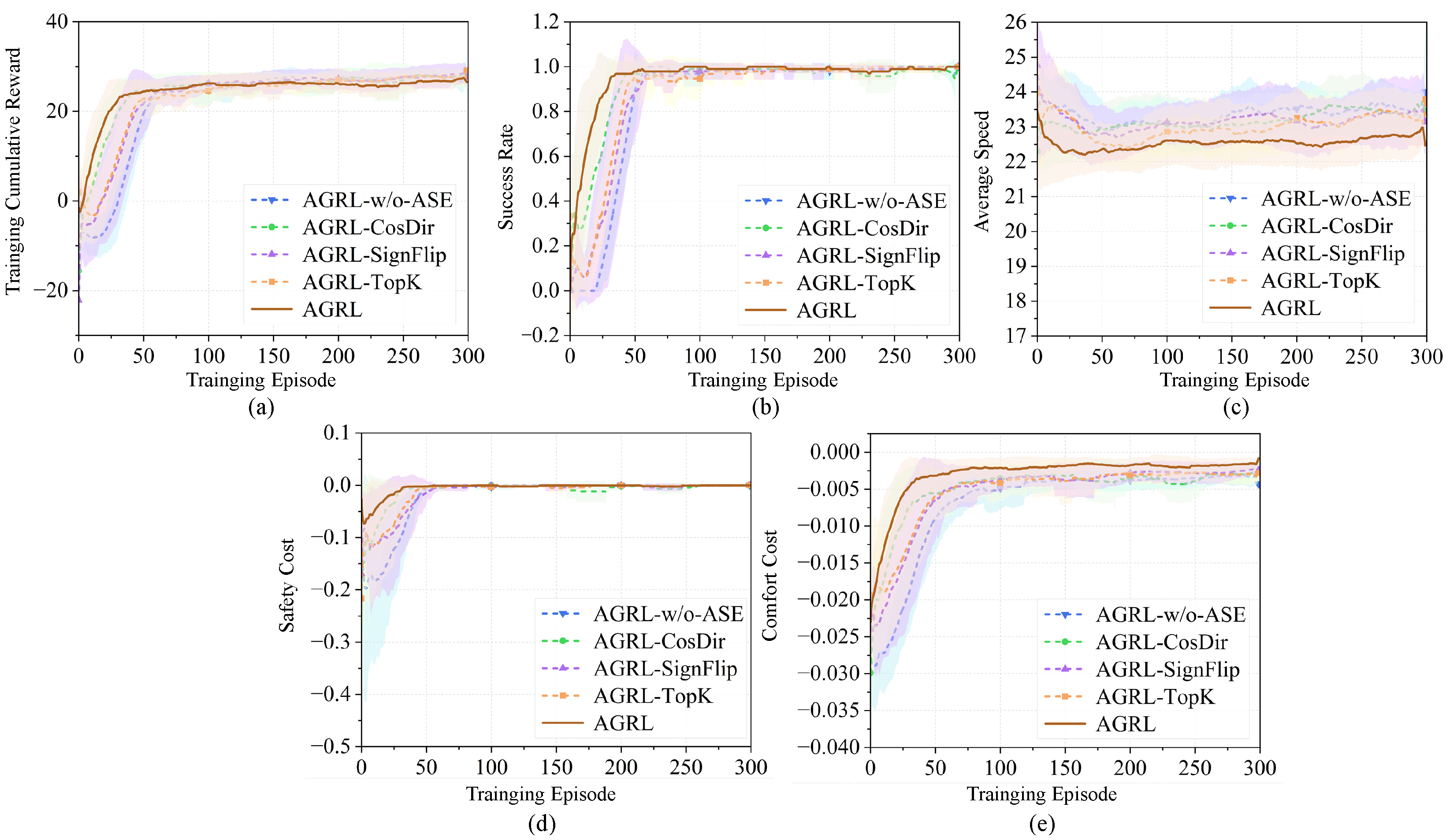
This experiment examines whether Euclidean attribution variation is more suitable for guiding exploration than other attribution-change metrics. Specifically, we compare five variants: AGRL, AGRL-CosDir, AGRL-SignFlip, AGRL-TopK, and AGRL-w/o-ASE. AGRL corresponds to the main exploration strategy used in the proposed method, where the Euclidean distance between the original and perturbed action-wise attribution vectors is used as the exploration signal. AGRL-CosDir uses the cosine-direction change between the two attribution vectors, AGRL-SignFlip uses the sign-flip ratio of attribution values, and AGRL-TopK uses the change in the top-k most important attribution features. AGRL-w/o-ASE removes the attribution-guided active exploration module and uses random exploration instead.

The ablation experiment is conducted in the highway lane-change scenario, and the results are shown in Figure 8. The results indicate that AGRL, which uses Euclidean attribution variation as the exploration signal, achieves the fastest convergence among all variants. In contrast, AGRL-w/o-ASE, which removes the attribution-guided active exploration module and relies on random exploration, shows the slowest convergence. This confirms that the attribution-guided exploration module contributes directly to improving learning efficiency.

Among the alternative attribution-change metrics, AGRL-CosDir achieves the closest performance to AGRL. This suggests that direction-related attribution information also has potential for guiding exploration. AGRL-SignFlip and AGRL-TopK also improve over AGRL-w/o-ASE to some extent, but their effects are weaker than those of AGRL and AGRL-CosDir. A possible reason is that the sign-flip ratio and top-k feature-overlap change are relatively discrete metrics. They may fail to capture fine-grained continuous changes in attribution magnitude, making the resulting exploration signal less stable and less informative. Overall, these results support the use of Euclidean attribution variation as the primary exploration signal in AGRL.

5.5. Interpretability Analysis in a Continuous Semantic Driving Scenario

To verify whether attribution variation reflects meaningful learned decision responses rather than random attribution noise or irrelevant feature interactions, we conduct a diagnostic interpretability analysis in a continuous semantic driving scenario.

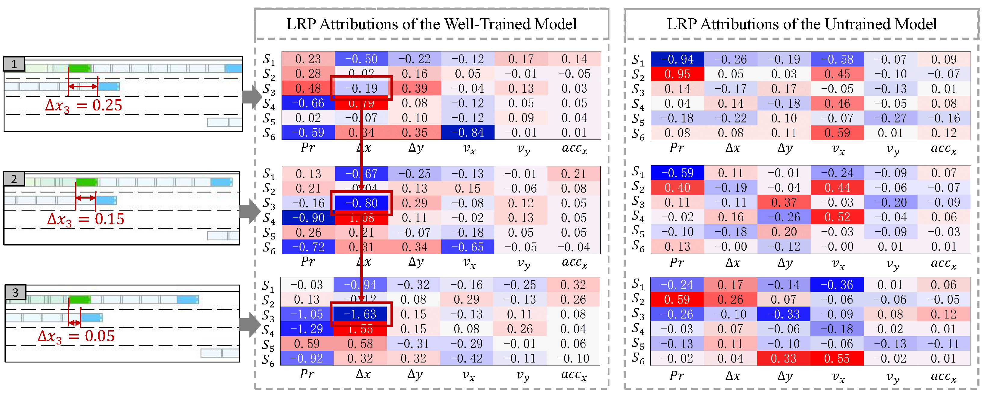
As shown in Figure 9, we select a continuous semantic driving scenario to compare the attribution changes of a well-trained policy and an untrained policy. In this scenario, the ego vehicle drives in the leftmost lane, while the longitudinal distance to the front-right vehicle, denoted as $\Delta x_3$, gradually decreases. We analyze the attribution heatmaps of the right-lane-change action.

The six rows in the heatmap represent the observations of the DRL agent: row 1 corresponds to the ego vehicle state, while rows 2 to 6 correspond to the states of the surrounding vehicles. Red indicates a positive contribution, blue indicates a negative contribution, and white represents a neutral or negligible contribution. These values indicate whether each feature supports or opposes the predicted advantage of the queried action.

For the well-trained policy, the attribution score associated with $\Delta x_3$ exhibits the most significant magnitude change, decreasing from $-0.19$ to $-1.63$. This is consistent with the driving semantics of the scenario: as the front-right vehicle becomes closer, the risk of executing a right-lane-change action increases, and the policy assigns a stronger negative attribution to the corresponding safety-critical feature. Therefore, the large Euclidean attribution variation in this case mainly reflects a meaningful magnitude response to increasing traffic risk. In contrast, the untrained policy does not exhibit such a semantically consistent attribution response.

To further quantify this phenomenon, we compute four attribution-change metrics among consecutive attribution vectors: Euclidean distance, cosine similarity, sign-flip rate, and top-5 feature overlap. The Euclidean distance measures the magnitude of attribution changes, while cosine similarity, sign-flip rate, and top-5 overlap characterize the consistency of attribution direction, sign pattern, and key feature selection, respectively. We report the average values over all three vector pairs in

Table 11. Quantitative comparison of attribution-change metrics between the well-trained and untrained models.

Model	Mean Euclidean Distance	Mean Cosine Similarity	Mean Sign-Flip Rate	Mean Top-5 Overlap
Well-trained	1.83	0.79	18.5%	73.3%
Untrained	1.44	0.48	35.2%	53.3%

.

The well-trained policy exhibits a larger mean Euclidean distance than the untrained policy, indicating stronger attribution-magnitude responses to the continuous change in the driving scenario. However, it also achieves higher cosine similarity, a lower sign-flip rate, and higher top-5 overlap. This means that the trained policy does not produce disordered attribution changes. Instead, it maintains a more consistent attribution direction and a more stable key-feature structure, while the attribution magnitudes of safety-critical features change more strongly. This finding supports that Euclidean attribution variation is a meaningful signal, as it reflects the response strength of the learned policy to continuous environmental changes rather than random or disordered attribution fluctuations.

6. Conclusions

In this work, we proposed an Attribution-Guided Reinforcement Learning (AGRL) framework for autonomous driving decision-making. The proposed method performs active exploration by evaluating perturbation-induced attribution sensitivity, allowing the agent to identify actions whose decision rationales are more locally responsive to state changes and to explore them in a targeted manner. Compared with conventional exploration-enhanced methods that rely on auxiliary predictive models or external novelty estimation, AGRL exploits the internal attribution signals of the decision model itself, making the exploration process more directly coupled to the policy’s local decision response. In addition, a global-attribution-based prior attention module is introduced to transfer attribution-derived prior knowledge from a pretrained interpretable policy to a new decision model, thereby accelerating learning in the early training stage.

This work highlights the potential of transforming attribution-based explainability from a post hoc analysis tool into an effective guidance signal for policy learning. Future work will focus on real-vehicle experiments to further validate the effectiveness and practical applicability of the proposed framework.

References

1. Wang, X.; Qi, X.; Wang, P.; Yang, J. Decision making framework for autonomous vehicles driving behavior in complex scenarios via hierarchical state machine. Auton. Intell. Syst. 2021, 1, 10. [Google Scholar] [CrossRef] [Scilit]
2. Fu, Y.; Li, C.; Yu, F.R.; Luan, T.H.; Zhang, Y. Hybrid autonomous driving guidance strategy combining deep reinforcement learning and expert system. IEEE Trans. Intell. Transp. Syst. 2021, 23, 11273–11286. [Google Scholar] [CrossRef] [Scilit]
3. Bae, S.H.; Joo, S.H.; Pyo, J.W.; Yoon, J.S.; Lee, K.; Kuc, T.Y. Finite state machine based vehicle system for autonomous driving in urban environments. In Proceedings of the 2020 20th International Conference on Control, Automation and Systems (ICCAS); IEEE: New York, NY, USA, 2020; pp. 1181–1186. [Google Scholar]
4. Omeiza, D.; Webb, H.; Jirotka, M.; Kunze, L. Explanations in autonomous driving: A survey. IEEE Trans. Intell. Transp. Syst. 2021, 23, 10142–10162. [Google Scholar] [CrossRef] [Scilit]
5. Li, X.; Bai, Y.; Cai, P.; Wen, L.; Fu, D.; Zhang, B.; Yang, X.; Cai, X.; Ma, T.; Guo, J.; et al. Towards knowledge-driven autonomous driving. arXiv 2023, arXiv:2312.04316. [Google Scholar] [CrossRef] [Scilit]
6. Jia, X.; Yang, Z.; Li, Q.; Zhang, Z.; Yan, J. Bench2drive: Towards multi-ability benchmarking of closed-loop end-to-end autonomous driving. Adv. Neural Inf. Process. Syst. 2024, 37, 819–844. [Google Scholar]
7. Sun, J.; Kim, J. Modelling two-dimensional driving behaviours at unsignalised intersection using multi-agent imitation learning. Transp. Res. Part C Emerg. Technol. 2024, 165, 104702. [Google Scholar] [CrossRef] [Scilit]
8. Huang, Z.; Sheng, Z.; Chen, S. PE-RLHF: Reinforcement Learning with Human Feedback and physics knowledge for safe and trustworthy autonomous driving. Transp. Res. Part C Emerg. Technol. 2025, 179, 105262. [Google Scholar] [CrossRef] [Scilit]
9. Huang, X.; Jing, P.; Li, Y.; Wang, X.; Wang, Y. Joint optimization of vehicle platoon and traffic signal with mixed traffic flow at intersections: Deep reinforcement learning approach. Transp. Res. Part C Emerg. Technol. 2025, 177, 105184. [Google Scholar] [CrossRef] [Scilit]
10. Zhou, R.; Huang, J.; Li, M.; Li, H.; Cao, H.; Song, X. Knowledge transfer from simple to complex: A safe and efficient reinforcement learning framework for autonomous driving decision-making. Adv. Eng. Inform. 2025, 65, 103188. [Google Scholar] [CrossRef] [Scilit]
11. Yang, K.; Tao, J.; Lyu, J.; Li, X. Exploration and anti-exploration with distributional random network distillation. arXiv 2024, arXiv:2401.09750. [Google Scholar] [CrossRef] [Scilit]
12. Shyam, P.; Jaśkowski, W.; Gomez, F. Model-based active exploration. In Proceedings of the International Conference on Machine Learning; PMLR: Tokyo, Japan, 2019; pp. 5779–5788. [Google Scholar]
13. Pathak, D.; Agrawal, P.; Efros, A.A.; Darrell, T. Curiosity-driven exploration by self-supervised prediction. In Proceedings of the International Conference on Machine Learning; PMLR: Tokyo, Japan, 2017; pp. 2778–2787. [Google Scholar]
14. Houthooft, R.; Chen, X.; Duan, Y.; Schulman, J.; De Turck, F.; Abbeel, P. Vime: Variational information maximizing exploration. Adv. Neural Inf. Process. Syst. 2016, 29. [Google Scholar]
15. Huang, J.; Zhou, R.; Li, M.; Li, H.; Liu, Y.; Song, X. From black-box to white-box: Interpretable deep reinforcement learning with Kolmogorov-Arnold networks for autonomous driving. Transp. Res. Part C Emerg. Technol. 2026, 182, 105386. [Google Scholar] [CrossRef] [Scilit]
16. Strehl, A.L.; Littman, M.L. An analysis of model-based interval estimation for Markov decision processes. J. Comput. Syst. Sci. 2008, 74, 1309–1331. [Google Scholar] [CrossRef] [Scilit]
17. Azar, M.G.; Osband, I.; Munos, R. Minimax regret bounds for reinforcement learning. In Proceedings of the International Conference on Machine Learning; PMLR: Tokyo, Japan, 2017; pp. 263–272. [Google Scholar]
18. Bellemare, M.; Srinivasan, S.; Ostrovski, G.; Schaul, T.; Saxton, D.; Munos, R. Unifying count-based exploration and intrinsic motivation. Adv. Neural Inf. Process. Syst. 2016, 29, 1479–1487. [Google Scholar]
19. Ostrovski, G.; Bellemare, M.G.; Oord, A.; Munos, R. Count-based exploration with neural density models. In Proceedings of the International Conference on Machine Learning; PMLR: Tokyo, Japan, 2017; pp. 2721–2730. [Google Scholar]
20. Machado, M.C.; Bellemare, M.G.; Bowling, M. Count-based exploration with the successor representation. In Proceedings of the AAAI Conference on Artificial Intelligence; IEEE: New York, NY, USA, 2020; Volume 34, pp. 5125–5133. [Google Scholar]
21. Lobel, S.; Bagaria, A.; Konidaris, G. Flipping coins to estimate pseudocounts for exploration in reinforcement learning. In Proceedings of the International Conference on Machine Learning; PMLR: Tokyo, Japan, 2023; pp. 22594–22613. [Google Scholar]
22. Burda, Y.; Edwards, H.; Storkey, A.; Klimov, O. Exploration by random network distillation. arXiv 2018, arXiv:1810.12894. [Google Scholar] [CrossRef] [Scilit]
23. Lundberg, S.M.; Lee, S.I. A Unified Approach to Interpreting Model Predictions. In Advances in Neural Information Processing Systems 30; Guyon, I., Luxburg, U.V., Bengio, S., Wallach, H., Fergus, R., Vishwanathan, S., Garnett, R., Eds.; Curran Associates, Inc.: New York, NY, USA, 2017; pp. 4765–4774. [Google Scholar]
24. Ribeiro, M.T.; Singh, S.; Guestrin, C. “Why should i trust you?” Explaining the predictions of any classifier. In Proceedings of the 22nd ACM SIGKDD International Conference on Knowledge Discovery and Data Mining; IEEE: New York, NY, USA, 2016; pp. 1135–1144. [Google Scholar]
25. Baehrens, D.; Schroeter, T.; Harmeling, S.; Kawanabe, M.; Hansen, K.; Müller, K.R. How to explain individual classification decisions. J. Mach. Learn. Res. 2010, 11, 1803–1831. [Google Scholar]
26. Khorram, S.; Lawson, T.; Fuxin, L. iGOS++ integrated gradient optimized saliency by bilateral perturbations. In Proceedings of the Conference on Health, Inference, and Learning; IEEE: New York, NY, USA, 2021; pp. 174–182. [Google Scholar]
27. Sundararajan, M.; Taly, A.; Yan, Q. Axiomatic attribution for deep networks. In Proceedings of the International Conference on Machine Learning; PMLR: Tokyo, Japan, 2017; pp. 3319–3328. [Google Scholar]
28. Smilkov, D.; Thorat, N.; Kim, B.; Viégas, F.; Wattenberg, M. Smoothgrad: Removing noise by adding noise. arXiv 2017, arXiv:1706.03825. [Google Scholar] [CrossRef] [Scilit]
29. Selvaraju, R.R.; Cogswell, M.; Das, A.; Vedantam, R.; Parikh, D.; Batra, D. Grad-cam: Visual explanations from deep networks via gradient-based localization. In Proceedings of the IEEE International Conference on Computer Vision; IEEE: New York, NY, USA, 2017; pp. 618–626. [Google Scholar]
30. Chattopadhay, A.; Sarkar, A.; Howlader, P.; Balasubramanian, V.N. Grad-cam++: Generalized gradient-based visual explanations for deep convolutional networks. In Proceedings of the 2018 IEEE Winter Conference on Applications of Computer Vision (WACV); IEEE: New York, NY, USA, 2018; pp. 839–847. [Google Scholar]
31. Montavon, G.; Binder, A.; Lapuschkin, S.; Samek, W.; Müller, K.R. Layer-wise relevance propagation: An overview. In Explainable AI: Interpreting, Explaining and Visualizing Deep Learning; Springer: Berlin/Heidelberg, Germany, 2019; pp. 193–209. [Google Scholar]
32. Li, J.; Zhang, C.; Zhou, J.T.; Fu, H.; Xia, S.; Hu, Q. Deep-LIFT: Deep label-specific feature learning for image annotation. IEEE Trans. Cybern. 2021, 52, 7732–7741. [Google Scholar] [CrossRef] [Scilit]
33. Wang, Z.; Schaul, T.; Hessel, M.; Hasselt, H.; Lanctot, M.; Freitas, N. Dueling network architectures for deep reinforcement learning. In Proceedings of the International Conference on Machine Learning; PMLR: Tokyo, Japan, 2016; pp. 1995–2003. [Google Scholar]
34. Leurent, E. An Environment for Autonomous Driving Decision-Making. 2018. Available online: https://github.com/eleurent/highway-env (accessed on 1 March 2026).
35. Bellotti, F.; Lazzaroni, L.; Capello, A.; Cossu, M.; De Gloria, A.; Berta, R. Explaining a deep reinforcement learning (DRL)-based automated driving agent in highway simulations. IEEE Access 2023, 11, 28522–28550. [Google Scholar] [CrossRef] [Scilit]
36. Treiber, M.; Hennecke, A.; Helbing, D. Congested traffic states in empirical observations and microscopic simulations. Phys. Rev. E 2000, 62, 1805. [Google Scholar] [CrossRef] [Scilit]
37. Kesting, A.; Treiber, M.; Helbing, D. General lane-changing model MOBIL for car-following models. Transp. Res. Rec. 2007, 1999, 86–94. [Google Scholar] [CrossRef] [Scilit]
38. Mnih, V.; Kavukcuoglu, K.; Silver, D.; Rusu, A.A.; Veness, J.; Bellemare, M.G.; Graves, A.; Riedmiller, M.; Fidjeland, A.K.; Ostrovski, G.; et al. Human-level control through deep reinforcement learning. Nature 2015, 518, 529–533. [Google Scholar] [CrossRef] [Scilit] [PubMed]
39. Van Hasselt, H.; Guez, A.; Silver, D. Deep reinforcement learning with double q-learning. In Proceedings of the AAAI Conference on Artificial Intelligence; IEEE: New York, NY, USA, 2016; Volume 30. [Google Scholar]
40. Tang, H.; Houthooft, R.; Foote, D.; Stooke, A.; Xi Chen, O.; Duan, Y.; Schulman, J.; DeTurck, F.; Abbeel, P. #Exploration: A study of count-based exploration for deep reinforcement learning. Adv. Neural Inf. Process. Syst. 2017, 30, 2750–2759. [Google Scholar]
Figure 1. Overview of the proposed AGRL framework.
Applsci 16 04931 g001
Figure 2. Overview of the proposed PAE-KAN. Local attribution explanations are first extracted from a well-trained KAN-based model over a large number of driving scenarios and then aggregated into a global explanation. The resulting global feature importance is subsequently embedded into a new PAE-KAN decision model as a global-attribution-based prior attention layer.
Applsci 16 04931 g002
Figure 3. Experimental driving scenarios. (a) Four-lane highway lane-change. (b) Main-road yielding. (c) On-ramp merging.
Applsci 16 04931 g003
Figure 4. Learning curves of autonomous driving agents in the highway lane-change scenario. (a) Training cumulative reward. (b) Success rate. (c) Average speed. (d) Safety cost. (e) Comfort cost.
Applsci 16 04931 g004
Figure 5. Learning curves of autonomous driving agents in the main-road yielding scenario. (a) Training cumulative reward. (b) Success rate. (c) Merge speed cost. (d) Safety cost. (e) Comfort cost. (f) Average speed.
Applsci 16 04931 g005
Figure 6. Learning curves of autonomous driving agents in the on-ramp merging scenario. (a) Training cumulative reward. (b) Success rate. (c) Average speed. (d) Safety cost. (e) Comfort cost.
Applsci 16 04931 g006
Figure 7. Training performance of different ablated versions of AGRL in the highway lane-change scenario. (a) Training cumulative reward. (b) Success rate. (c) Average speed. (d) Safety cost. (e) Comfort cost.
Applsci 16 04931 g007
Figure 8. Ablation study of different attribution-based exploration signals in the highway lane-change scenario. (a) Training cumulative reward. (b) Success rate. (c) Average speed. (d) Safety cost. (e) Comfort cost.
Applsci 16 04931 g008
Figure 9. LRP-KAN attribution responses in a continuous semantic driving scenario. The red arrows indicate changes in attribution responses.
Applsci 16 04931 g009