Stability-Aware Uplift Policy Selection for Customer Retention: From Predictive Scores to Actionable Segments

Abstract

Uplift modeling optimizes intervention-based campaigns by identifying customers whose behavior changes exclusively due to specific treatments, moving beyond standard baseline risk predictions. However, in real-world deployments, algorithms that maximize traditional causal ranking metrics (e.g., the Qini coefficient) often fail to be optimal in practice. The inherent variance of Conditional Average Treatment Effect (CATE) estimators exposes critical trade-offs between expected economic value, algorithmic stability, and policy interpretability. To address this gap, this study proposes a stability-aware, value-driven computational framework for selecting an uplift policy. The pipeline evaluates multiple causal and non-causal algorithmic families, including traditional baselines, multimodel approaches, and transformed-outcome variants, within a repeated-run validation protocol. Candidate policies are assessed primarily through incremental revenue and target-set stability, whereas a post hoc surrogate tree distillation step is used to translate the selected policy into interpretable rule-based customer segments. An empirical evaluation of the publicly available Telco Customer Churn dataset under two distinct regimes (a causally controlled semisynthetic scenario and an observational proxy scenario) reveals that the highest-yielding causal policy frequently suffers from severe targeting instability, inducing a clear risk–return trade-off. Furthermore, uplift models outperform traditional baselines in the causally controlled regime, whereas traditional baselines remain economically superior in the confounded proxy settings. Overall, this study establishes that jointly assessing economic utility, algorithmic stability, and transparent segmentation is essential for deploying robust and defensible causal machine learning in production environments.

1. Introduction

Customer retention is a central decision problem in subscription-based industries, such as telecommunications, where firms allocate substantial resources to discounts, offers, and contact strategies to reduce churn. In this setting, the relevant analytical question is not only which customers are likely to leave, but also which customers are likely to modify their behavior as a direct result of an intervention. This fundamental distinction separates conventional churn modeling from uplift modeling. While standard predictive models rank customers by baseline response propensity, uplift modeling seeks to identify customers for whom a treatment is expected to generate real incremental value.

A conventional churn model may prioritize customers who would remain (sure things), leave regardless (lost causes), or even react negatively to the contact by churning when they otherwise would not have (sleeping dogs). By allocating budgets to low-value or actively harmful interventions, conventional models fail to isolate customers who are persuadable. For this reason, recent literature increasingly treats uplift modeling not merely as a treatment effect estimation problem, but as a broader decision problem in which prediction, policy design, and treatment allocation must be optimized jointly [1,2,3,4,5]. In parallel, segmentation-oriented research emphasizes that deployable uplift systems must remain interpretable, ensuring that targeting decisions can be translated into understandable operational rules rather than opaque mathematical scores [6].

Over the last decade, the uplift literature has significantly expanded. Foundational reviews have organized the field around transformation-based methods, two-model approaches, and direct uplift algorithms, highlighting the strengths and empirical sensitivity of these techniques [1,7]. Subsequent work has extended the methodology toward value-driven evaluation, multi-treatment settings, advanced causal machine learning architectures, and contextual real-time applications [8,9,10,11]. Taken together, these studies substantially advance CATE estimation. However, they also make it clear that an accurate mathematical estimation does not automatically yield a policy that is economically preferable, operationally reproducible, and easy to communicate to decision makers.

This positioning also distinguishes the present work from recent causal machine learning policy optimization frameworks. Such frameworks typically focus on directly learning or optimizing individualized treatment rules, for example through welfare-based policy learning, predict-then-optimize formulations, causal-forest-based targeting, contextual bandits, or reinforcement learning for sequential interventions [4,5,12,13]. The objective of this paper is different. We do not introduce a new CATE estimator, nor do we optimize a dynamic sequence of marketing actions. Instead, we propose a deployment-oriented selection and audit layer that compares candidate uplift policies under a common validation protocol, using realized economic value, run-to-run customer-list stability, and post hoc interpretability as joint decision criteria.

Despite this progress, two major obstacles limit the practical deployment of uplift methods in production settings. The first is objective function misalignment: the algorithm that maximizes standard causal ranking metrics (e.g., Qini or Area Under the Uplift Curve) does not necessarily maximize the downstream business objective, such as expected incremental revenue. The second is policy instability: the identity of the targeted and persuadable customers may vary substantially across repeated training runs, random data splits, or equivalent model specifications. In practical campaign settings, highly volatile policies are difficult to trust, audit, and operationalize. As the retention literature has demonstrated, targeting customers solely based on high-risk scores is highly ineffective when they are intrinsically unresponsive to treatment [14].

Against this background, this study evaluates uplift modeling as a deployment-oriented decision problem, rather than relying solely on ranking metrics. We develop a stability-aware and business-aligned framework for selecting retention policies. The framework does not assume that uplift models always outperform conventional response models. Instead, it tests when uplift-based targeting is economically useful, stable across repeated runs, and interpretable enough for operational deployment.

To this objective, we evaluate the framework on a telecommunications churn dataset under two complementary regimes. The primary regime is a causally controlled semisynthetic benchmark. The secondary regime is an observational contract-proxy scenario based on month-to-month contracts. Within this common environment, we compare a traditional response baseline, two-model uplift learning, treatment-indicator learning, four-quadrant modeling, and transformed-outcome variants.

This study contributes to the uplift modeling and customer-retention literature by connecting causal policy evaluation with deployment-oriented business requirements. Its main contributions are summarized as follows.

• We integrate economic value and algorithmic stability into uplift policy evaluation, assessing candidate policies through incremental revenue and target-set reproducibility rather than relying only on causal ranking metrics.
• We introduce a repeated-run validation framework that quantifies the stability of targeted and persuadable customer sets across random data splits and model refits.
• We add a post hoc distillation stage that converts complex uplift scores into interpretable rule-based customer segments suitable for CRM deployment.

The remainder of this paper is organized as follows. Section 2 reviews the literature on uplift modeling, decision-oriented policy design, and interpretable segmentation. Section 3 formalizes the proposed framework. Section 4 describes the experimental protocols and datasets. Section 5 presents the comparative performance, stability analysis, and distilled policy segments of the proposed method. Section 6 discusses the methodological and managerial implications of the study. Section 7 concludes the paper.

2. Related Work

Uplift modeling addresses intervention-based decision problems in which the objective is not only to predict an outcome but also to estimate how that outcome changes with treatment. In customer retention and campaign optimization, this distinction is fundamental: the decision-maker is interested in identifying customers whose behavior can be positively influenced by an intervention rather than customers who are simply likely to respond or remain. Therefore, uplift modeling occupies an intermediate position between causal inference, predictive analytics, and prescriptive decision-making support. A review of the literature reveals several major research streams in the current state of the art.

2.1. Foundations and Positioning

Foundational survey papers have framed uplift modeling as a bridge between causal inference and prescriptive analytics, organizing the field around transformation-based methods, two-model approaches, and direct uplift modeling [1,7]. These reviews emphasize that uplift methods are highly sensitive to data characteristics, modeling choices, and evaluation design. Furthermore, metrics such as Qini curves and related cumulative-gain measures, while standard, do not always align naturally with business objectives [1,15,16,17]. A conceptual pillar underlying all of these methods is the four-quadrant customer taxonomy (persuadable, sure things, lost causes, and sleeping dogs) which represents the theoretical motivation for separating uplift from conventional response scoring [1].

2.2. Core Methodological Strategies

Classical uplift work includes the two-model approach (T-learner), where separate models are estimated for treatment and control groups, and class-transformation or transformed-outcome methods, in which the target is recoded so that standard supervised learners can approximate treatment effect heterogeneity [7,18]. Another major family consists of direct uplift models, especially tree-based methods, designed to separate treatment-sensitive and treatment-insensitive regions directly during learning [19]. Ensemble extensions improve predictive discrimination while preserving some degree of segment interpretability [20].

A recent codification of the transformed-outcome approach (TOA) is provided by Pinheiro and Cavique [6], who formalize $Y^{★}$ as a binary variable equal to 1 for persuadable customers and 0 for defiers. They demonstrated that modeling the conditional distribution of $Y^{★}$ is mathematically equivalent to directly estimating the conditional uplift, providing a robust statistical foundation for deploying standard classifiers (e.g., logistic regression) to optimize causal targets.

2.3. Connection to Causal Machine Learning

Uplift estimation is closely related to Conditional Average Treatment Effect (CATE) estimation, as both quantify how treatment effects vary across individuals or subpopulations [21]. Recent causal machine learning research has significantly expanded the algorithmic toolkit with meta-learners and representation learning approaches [22,23,24]. Neural architectures, such as Dragonnet and related deep causal models, demonstrate that flexible nonlinear learners can improve treatment effect estimation when covariate interactions are complex and the imbalance between treatment groups must be explicitly controlled [25].

Deep neural extensions of the classical uplift evaluation paradigm have recently been proposed by Ramachandra [26], who introduced QiniDeep, a Deep Uplift Network architecture featuring a shared representation trunk with multiple output heads for each treatment arm. This multi-head architecture enables the joint estimation of all potential outcomes within a single forward pass, significantly improving information sharing compared to independently trained T-learner networks. Benchmarks show that QiniDeep achieves lower PEHE (Precision in Estimation of Heterogeneous Effects) and a superior Qini coefficient compared to causal forests. The authors highlighted that overfitting represents a severe practical risk for deep uplift models, which directly motivates the stability-aware evaluation protocol proposed in the present study.

2.4. Business-Oriented and Multi-Treatment Evaluation

Benchmark studies in campaign optimization have compared classic uplift strategies in realistic purchase-response settings and shown that model rankings depend heavily on the selected business objective [8,9]. In parallel, multi-treatment uplift modeling has extended the classical binary setup toward richer intervention settings, including multiple treatments and more general response types [10,27].

2.5. Decision Alignment and Policy Design

The ultimate objective is rarely uplift in isolation, but rather a utility criterion, such as incremental revenue, profit, or resource-constrained policy benefits. The most accurate treatment effect model is not automatically the model that yields the best deployable policy [4]. This perspective is explicitly developed in predict-then-optimize uplift frameworks, where estimation is treated as a step in a broader policy-design pipeline.

The most formally complete instantiation of this paradigm in recent literature is provided by De Vos et al. [5], who extended uplift modeling to continuous treatments by separating the problem into (i) a prediction step that estimates conditional average dose responses and (ii) an optimization step formulated as an Integer Linear Programming problem. Critically, De Vos et al. demonstrated a systematic misalignment between estimation quality (measured by the Mean Integrated Squared Error) and downstream policy value (measured by the Area Under the Uplift Curve). This empirical result directly reinforces the central premise of this study: optimizing estimation accuracy and policy value are mathematically distinct objectives that require separate evaluation stages.

2.6. Interpretability and Segmentation

Although many uplift studies focus on predictive accuracy, practical deployment often requires a transparent model. To this end, Pinheiro and Cavique [6] proposed a reproducible two-phase framework that emphasizes actionable segment discovery. A key contribution of their work is the formal distinction between scoring models (which produce iso-cardinality strata) and partitioning models (which produce hetero-cardinality strata defined by decision tree leaves). The latter provides interpretable Boolean rules, such as tenure $\in [34,46]$ AND streamingMovies $=0$, which are directly actionable in enterprise CRM systems without requiring a continuous numerical score. This segment-centric logic directly inspires the post hoc distillation stage of the framework presented in this study, which is consistent with the operational need to isolate persuadable customers while avoiding potentially harmful interventions.

2.7. Deep and Industrial Uplift Modeling

In large-scale digital systems, uplift estimation increasingly involves rich contextual information and distribution shifts between treatment and control groups. Sun et al. [11] introduced the UMLC framework (Robust Uplift Modeling with Large-Scale Contexts), addressing the specific challenge of real-time marketing, where each user interacts with numerous distinct context items per session. They demonstrated that grouping contextual embeddings mitigates the severe distribution shift that is inherent in observational industrial data. Their findings underscore a critical deployment consideration: the choice of context granularity directly determines the variance–bias trade-off in uplift estimation. This context-dependent instability is analogous to the run-to-run Jaccard instability documented in the simplified tabular setting of this study. Hence, the stability layer proposed here will become even more critical as models scale to high-dimensional contextual-input spaces.

2.8. Gap in the Literature

The literature has made substantial progress in foundational taxonomies, causal machine learning estimators, business-oriented evaluations, and interpretable deployment frameworks [1,6,9,11]. However, most studies prioritize treatment effect ranking quality over algorithmic stability. In real-world deployments, the instability of the targeted customer set across repeated training runs is a significant limitation. Second, there is a lack of end-to-end methodologies that jointly formalize business-aligned evaluation, repeated-run robustness, and post hoc segment extraction within a single pipeline.

The present study is positioned at this intersection of research. Relative to policy-learning and predict-then-optimize frameworks [4,5,12], it does not attempt to solve a new constrained treatment-allocation problem. Instead, it asks whether the policy produced by a candidate uplift model remains economically valuable and operationally reproducible when the full training–validation–testing pipeline is repeated. Relative to dynamic marketing optimization frameworks based on causal forests, contextual bandits, or reinforcement learning [13], the proposed framework is deliberately simpler and batch-oriented: it is designed for firms that need to choose, justify, and deploy a stable customer list for a retention campaign, rather than continuously optimize a sequence of interventions. Relative to segmentation-oriented studies [6], it adds an explicit repeated-run stability diagnostic and a value-driven policy-selection criterion. Ultimately, this study argues that the most relevant empirical question is not whether a method attains the highest average Qini coefficient, but whether it yields an economically defensible, sufficiently stable, and interpretable targeting policy.

3. Methodology

3.1. Problem Setting

We consider a binary customer retention intervention problem. Let $X\in \mathcal{X}$ denote the customer feature vector, $T\in \{0,1\}$ the treatment assignment, and $Y\in \{0,1\}$ the observed retention outcome, with $Y=1$ representing a positive retention. Let $Y\left(1\right)$ and $Y\left(0\right)$ denote the potential outcomes under the treatment and control conditions, respectively. The fundamental causal quantity of interest is the Conditional Average Treatment Effect (CATE):

$$\tau \left(x\right)=\mathbb{E}\left[Y\right(1)-Y(0)\mid X=x].$$

(1)

Because Y is binary, $\tau \left(x\right)$ also coincides with the difference in conditional response probabilities whenever the causal effect is identified:

$$\tau \left(x\right)=Pr(Y=1\mid T=1,X=x)-Pr(Y=1\mid T=0,X=x).$$

(2)

In the semisynthetic regime, $\tau \left(x\right)$ is point-identified because the treatment is randomized by construction, and the response probabilities under treatment and control are explicitly generated. In contrast, in the contract proxy regime, consistency, conditional ignorability, and overlap remain identifying assumptions rather than empirically verifiable facts that can be tested. Therefore, inverse propensity weighting is used only as a bias-reduction device in proxy economic evaluation, not as proof that the full learning problem is causally identified.

The practical objective is not only to estimate treatment sensitivity but also to derive a deployable targeting policy. For model m and target fraction $f\in (0,1]$, the corresponding binary policy is defined as

$${\pi }_{m,f}\left(x\right)=\mathbb{I}\{s_m\left(x\right)\ge c_{m,f}\},$$

(3)

where $s_m\left(x\right)$ is the model-specific predictive score, and $c_{m,f}$ is the threshold chosen so that the policy targets the top-f fraction of customers according to that score.

Let

$${\mathcal{T}}_f\left(m\right)=\{i:s_m\left(x_i\right)\ge c_{m,f}\}$$

(4)

denote the target set induced by model m at fraction f. To characterize the subset of targeted customers predicted to benefit from treatment, we introduce a model-specific signed uplift score $u_m\left(x\right)$, whose sign is interpreted as the predicted direction of the incremental effect. When the model directly estimates the CATE, we set $u_m\left(x\right)={\widehat{\tau }}_m\left(x\right)$; otherwise, $u_m\left(x\right)$ denotes the corresponding signed uplift-oriented score produced by the model. The persuadable subset is then defined as

$${\mathcal{P}}_f\left(m\right)=\{i\in {\mathcal{T}}_f\left(m\right):u_m\left(x_i\right)>0\}.$$

(5)

For the traditional baseline (Model 1), which does not produce a signed uplift score, the persuadable set coincides with the target set by convention. In the empirical study, candidate policies were evaluated primarily through downstream incremental revenue rather than uplift-ranking metrics alone.

This policy formulation is deliberately discrete and budget-constrained, consistent with the operational requirements of customer retention campaigns. Extensions to continuous treatment intensity and unconstrained optimization are possible but are outside the scope of this study, which focuses on the stability and interpretability of binary targeting policies.

An empirical analysis was conducted on a telecommunications churn dataset. To evaluate the algorithms without a randomized controlled trial, the computational framework operates in two complementary regimes. The primary regime, a semisynthetic scenario, generates a controlled causal environment from the observed customer covariates. The secondary regime, the contract proxy scenario, treats month-to-month contracts as an observational proxy for intervention and applies inverse propensity weighting to partially mitigate treatment-selection bias in the economic evaluation. This dual design supports a deployment-oriented comparison between controlled causal benchmarking and observational proxy assessments. The two empirical regimes used in the experiments are dataset-specific and are described in Section 4.1.

3.2. Compared Model Families

The computational pipeline compares seven model instances that are grouped into five conceptual families. The purpose is not to advocate a single universal learner but to compare distinct uplift-oriented scoring logics under a repeated-run evaluation protocol.

The selected models were chosen to span distinct and widely used methodological families in uplift modeling and CATE estimation, enabling a systematic comparison of alternative scoring logics under a unified validation protocol. Model 1 represents a non-uplift response-oriented targeting benchmark [28]. Models 2 and 3 represent meta-learner CATE formulations, namely the T-learner/two-model and S-learner strategies [15,22,29]. Model 4 represents the true-lift and four-quadrant tradition [15,28]. Models 5–7 represent transformed-outcome or class-transformation approaches, implemented with simple alternative base learners to compare smooth and rule-based variants [8,18]. The goal is comparative methodological coverage, not the introduction of new estimators or an exhaustive benchmark of all possible learners.

Table 1. Summary of the compared model families, ranking scores, and interpretation caveats.

Model	Family	Score Used for Ranking	Main Assumption or Caveat
Model 1	Naïve response- oriented comparator	$\widehat{Pr}(T=1,Y=1\mid X=x)$	Not a CATE estimator; used only as a conventional targeting benchmark.
Model 2	Two-model uplift/T-learner	${\widehat{p}}_1\left(x\right)-{\widehat{p}}_0\left(x\right)$	Requires sufficient support in both treatment groups; subtracting two independent learners may increase variance.
Model 3	Treatment-indicator model/S-learner	$\widehat{g}(x,1)-\widehat{g}(x,0)$	Uses one outcome model with treatment as an input; may smooth weak treatment heterogeneity.
Model 4	Four-quadrant uplift model	$(q_{\mathrm{TR}}\left(x\right)+q_{\mathrm{CR}}\left(x\right))-(q_{\mathrm{CR}}\left(x\right)+q_{\mathrm{TN}}\left(x\right))$	Preserves the treatment–response taxonomy; should be interpreted as an uplift-oriented proxy rather than a direct latent-type estimator.
Model 5	Transformed outcome with logistic regression	$\widehat{Pr}(Y^{★}=1\mid X=x)$	Monotonic in uplift under balanced randomized assignment; sensitive to imbalance or confounding in observational settings.
Model 6	Transformed outcome with discriminant analysis	$\widehat{Pr}(Y^{★}=1\mid X=x)$	Same transformation as Model 5, with additional linear-discriminant modeling assumptions.
Model 7	Transformed outcome with shallow decision tree	$\widehat{Pr}(Y^{★}=1\mid X=x)$	Provides simple nonlinear partitions, but may be sensitive to small sample changes.

The score is used only to rank customers and define the top-f target set. Economic value is evaluated subsequently through the validation-based incremental-revenue criterion.

summarizes the seven implemented models, the ranking score used by each policy, and the main assumptions or interpretation caveats associated with each family.

3.2.1. Model 1: Traditional Baseline

Model 1 serves as a naïve response-oriented benchmark. In the implemented pipeline, it does not estimate a CATE and does not even fit a standard churn model of the form $Pr(Y=1\mid X=x)$. Instead, it trains a binary classifier for the event

$$s_1\left(x\right)\approx Pr(T=1,Y=1\mid X=x),$$

(6)

that is, the probability of belonging to the observed class of treated responders. Therefore, it is included only as a practical baseline score for targeting, not as a real uplift estimator. This distinction is important because its Qini- and AUQC-based metrics are not directly comparable to those of the uplift models.

3.2.2. Model 2: Two-Model Uplift (T-Learner)

Model 2 fits two separate supervised response models, one for the treated subgroup and one for the control subgroup:

$${\widehat{p}}_1\left(x\right)=\widehat{Pr}(Y=1\mid T=1,X=x),{\widehat{p}}_0\left(x\right)=\widehat{Pr}(Y=1\mid T=0,X=x).$$

(7)

Its uplift score is the difference

$${\widehat{\tau }}_2\left(x\right)={\widehat{p}}_1\left(x\right)-{\widehat{p}}_0\left(x\right).$$

(8)

This is a canonical T-learner architecture. Its main weakness is variance inflation because the two models are trained independently, and their difference may become unstable in sparsely supported regions of the feature space.

3.2.3. Model 3: Treatment-Indicator Model (S-Learner)

Model 3 fits a single supervised learner with the treatment indicator appended to the feature vector. Let $\widehat{g}(x,t)$ denote the fitted conditional response model; the uplift score is then obtained by counterfactual scoring:

$${\widehat{\tau }}_3\left(x\right)=\widehat{g}(x,1)-\widehat{g}(x,0).$$

(9)

This S-learner avoids the explicit subtraction of two separately trained models; however, it may understate treatment heterogeneity when the main response signal dominates the treatment effect.

3.2.4. Model 4: Four-Quadrant Model

Model 4 recasts the problem as a multi-class classification over the four observed treatment–response combinations. Let

$$q_{\mathrm{TR}}\left(x\right),q_{\mathrm{CR}}\left(x\right),q_{\mathrm{CR}}\left(x\right),q_{\mathrm{TN}}\left(x\right)$$

denote the estimated probabilities of the observed classes treated responder, control responder, control non-responder, and treated non-responder, respectively. The model score is

$${\widehat{\tau }}_4\left(x\right)=\left(q_{\mathrm{TR}}\left(x\right)+q_{\mathrm{CR}}\left(x\right)\right)-\left(q_{\mathrm{CR}}\left(x\right)+q_{\mathrm{TN}}\left(x\right)\right).$$

(10)

Because the four class probabilities sum to one, this can also be written as

$${\widehat{\tau }}_4\left(x\right)=2\left(q_{\mathrm{TR}}\left(x\right)+q_{\mathrm{CN}}\left(x\right)\right)-1.$$

(11)

This score should be interpreted as an uplift-oriented proxy derived from the observed treatment–response quadrants. It preserves the full four-cell taxonomy and supports an operational segmentation view, but should not be read as a direct estimator of latent causal customer types.

3.2.5. Models 5–7: Transformed-Outcome Models

The final family applies a binary target transformation so that a standard classifier can be used to produce an uplift-oriented order. The transformed outcome is defined as

$$Y^{★}=\left\{\begin{array}{cc}1,\hfill & \mathrm{if}(T=1\wedge Y=1)\vee (T=0\wedge Y=0),\hfill \\ 0,\hfill & \mathrm{otherwise}.\hfill \end{array}\right.$$

(12)

Thus, $Y^{★}=1$ collects the observed treatment–response combinations $(\mathrm{TR},\mathrm{CN})$, whereas $Y^{★}=0$ collects $(\mathrm{CR},\mathrm{TN})$. Under balanced randomization with $Pr(T=1\mid X=x)=0.5$,

$$Pr(Y^{★}=1\mid X=x)=\frac{1}{2}\left(1+\tau \left(x\right)\right),$$

(13)

so $Pr(Y^{★}=1\mid X=x)$ is monotonic in the underlying uplift $\tau \left(x\right)$. In the same regime, Equation (11) shows that the four-quadrant score is an affine transformation of the same quantity. For Models 5–7, the ranking score is $s_m\left(x\right)=\widehat{Pr}(Y^{★}=1\mid X=x)$. The signed score used in the persuadable-set definitions is instead $u_m\left(x\right)=2s_m\left(x\right)-1$, which preserves the same customer ordering while making the threshold $u_m\left(x\right)>0$ correspond to positive predicted uplift under balanced randomized assignment.

This population-level equivalence does not, however, imply identical finite-sample behavior: the four-class logistic estimator of Model 4 allocates parameters across all four cells simultaneously, while the binary logistic estimator of Models 5–7 operates on the collapsed $Y^{★}$ label, yielding different estimation variance even under randomization. Moreover, in observational or strongly unbalanced settings, neither score should be treated as a direct CATE estimator without explicit propensity correction in the learning step.

Within this transformed-outcome family, the framework evaluates three classifier variants: logistic regression (Model 5), discriminant analysis (Model 6), and a shallow decision tree (Model 7). This allows the analysis to isolate the effect of the base learner while keeping the transformed-outcome architecture fixed.

3.3. Validation-Based Policy Selection

For each model m, customer-level scores are first computed on the validation set and then converted into candidate policies by targeting the highest-ranked customers. Let

$$\mathcal{F}=\{0.03,0.05,0.07,0.09,0.12,0.15\}$$

(14)

denote the discrete search space of the target fractions. For a given fraction $f\in \mathcal{F}$, policy ${\pi }_{m,f}$ targets the top-f fraction of validation customers according to the model score $s_m\left(x\right)$. Thus, the score is used only to rank customers; the economic value of the policy is evaluated later.

Let D denote a generic evaluation sample, which may be either a validation or test set. For model m and fraction f, define

$$n_T^D(m,f)=\sum _{i\in D}{\pi }_{m,f}\left(x_i\right)$$

as the number of targeted customers in D. The policy value is then computed in a scenario-specific manner.

In the semisynthetic regime, the response probabilities under treatment and control are known for each customer. The incremental revenue of policy ${\pi }_{m,f}$ on sample D is

$${\mathrm{IR}}_D^{\mathrm{semi}}(m,f)=V\sum _{i\in D}{\pi }_{m,f}\left(x_i\right)\left(p_1\left(x_i\right)-p_0\left(x_i\right)\right)-C\sum _{i\in D}{\pi }_{m,f}\left(x_i\right),$$

(15)

where $p_1\left(x_i\right)$ and $p_0\left(x_i\right)$ denote the known semisynthetic response probabilities under treatment and control, respectively. The constants V and C are business-calibration parameters: V is the gross monetary value assigned to one additional retained customer, whereas C is the unit cost incurred for applying the retention action to one targeted customer. Both constants are expressed in the same monetary units as incremental revenue.

In the contract proxy regime, the economic value of the policy is estimated by inverse propensity weighting on the targeted subset. Let

$$A_D(m,f)=\{i\in D:{\pi }_{m,f}\left(x_i\right)=1\}$$

denote the set of customers targeted by policy ${\pi }_{m,f}$ on sample D. Then,

$${\widehat{\mathrm{IR}}}_D^{\mathrm{proxy}}(m,f)=V{n}_T^D(m,f)\left({\widehat{\mu }}_{1,D}^{\mathrm{IPW}}(m,f)-{\widehat{\mu }}_{0,D}^{\mathrm{IPW}}(m,f)\right)-C{n}_T^D(m,f),$$

(16)

where the treated and control outcome rates within the targeted subset are estimated as

$${\widehat{\mu }}_{1,D}^{\mathrm{IPW}}(m,f)={\displaystyle \frac{{\sum }_{i\in A_D(m,f)}{w}_i^{\left(1\right)}{Y}_i}{{\sum }_{i\in A_D(m,f)}{w}_i^{\left(1\right)}}},{\widehat{\mu }}_{0,D}^{\mathrm{IPW}}(m,f)={\displaystyle \frac{{\sum }_{i\in A_D(m,f)}{w}_i^{\left(0\right)}{Y}_i}{{\sum }_{i\in A_D(m,f)}{w}_i^{\left(0\right)}}},$$

(17)

with inverse propensity weights

$$w_i^{\left(1\right)}={\displaystyle \frac{T_i}{\tilde{e}\left(x_i\right)}},w_i^{\left(0\right)}={\displaystyle \frac{1-T_i}{1-\tilde{e}\left(x_i\right)}},$$

(18)

and clipped propensity score

$$\tilde{e}\left(x_i\right)=min\{0.95,max(0.05,\widehat{e}\left(x_i\right))\}.$$

(19)

When the model score correlates strongly with T (as expected in the contract proxy regime), small target fractions may yield a targeted set $A_D(m,f)$ dominated by treated customers, leaving very few control observations to inform ${\widehat{\mu }}_{0,D}^{\mathrm{IPW}}$. Propensity clipping partially mitigates extreme weight inflation but does not remove the finite-sample instability of the estimator when the treatment overlap within $A_D(m,f)$ is poor. This is a limitation of the proxy economic evaluation and represents an additional reason why the proxy results should be interpreted with greater caution than the semisynthetic benchmark.

The same economic criterion is used on the validation set to select the target fraction and on the test set to report out-of-sample results. The difference is purely functional: validation is used for policy selection, whereas the test is used only for the final evaluation.

For each model, the primary validation value-maximizing fraction is denoted as $f_m^{IR}$. In compact notation,

$$f_m^{IR}\in arg\underset{f\in \mathcal{F}}{max}{\mathrm{IR}}_{D_{\mathrm{val}}}(m,f),$$

(20)

where ${\mathrm{IR}}_{D_{\mathrm{val}}}(m,f)$ is the appropriate validation criterion: Equation (15) in the semisynthetic regime and Equation (16) in the proxy regime. The implemented selected fraction $f_m^{★}$ is then obtained by applying the operational refinement described below to this primary incremental-revenue criterion. First, only candidate fractions of at least $0.03$ are considered; in the present study, this condition is automatically satisfied by all values in Equation (14). Second, if at least one candidate policy yields a positive validation incremental revenue, only the policies whose value is at least 95% of the best positive value are retained. Among these near-best profitable candidates, the selected policy is the one with the highest incremental revenue per euro spent. If no candidate policy yields a positive validation incremental revenue, the selected fraction is the one with the highest validation incremental revenue.

The economic constants were calibrated ex ante and fixed throughout the experiments at $V=180$ and $C=15$, corresponding to a value-to-cost ratio of 12 and to a break-even uplift threshold $C/V=0.083$. Thus, a targeted policy generates positive expected incremental revenue only when the average uplift among targeted customers exceeds approximately 8.3 percentage points. Keeping these values fixed across random seeds, model families, scenarios, and target fractions ensures that differences in the reported incremental revenue are driven by the learned policies rather than by changes in the business payoff assumptions. Since Equations (15) and (16) are linear in V and C, increasing V rewards policies that identify larger positive treatment effects, whereas increasing C penalizes broader targeting and may shift the validation-selected fraction toward smaller customer lists. Although Qini, AUQC, and Uplift@K are also computed to assess ranking quality, incremental revenue is the primary criterion used to select the deployable policy.

3.4. Repeated-Run Stability Layer

A central component of the framework is a repeated-run stability analysis. Rather than evaluating the models on a single train–validation–test split, the entire pipeline is repeated over multiple random seeds. For each model and run, the algorithm stores the test-sample customer identifiers, together with the binary targeting decisions and binary persuadable labels.

Importantly, the stability quantities reported in this study should not be interpreted as intrinsic, context-free properties of the algorithms. They are conditional estimates of policy reproducibility under a specific empirical regime, feature space, sample size, outcome prevalence, treatment-assignment mechanism, base-learner specification, and validation-based targeting rule. The Jaccard indices quantify the interaction between a model family and the statistical properties of the dataset under analysis. The same algorithm may appear stable when the treatment effect signal is strong and well separated, but unstable when the signal is weak, outcomes are sparse, covariates are highly imbalanced, or customer profiles differ across domains.

For a fixed model m, consider two runs $r_a$ and $r_b$. Because the two test sets are not identical, stability is evaluated only for the customers that appear in both.

$$D_{ab}^{\left(m\right)}=D_{\mathrm{test}}^{\left(r_a\right)}\cap D_{\mathrm{test}}^{\left(r_b\right)}.$$

(21)

On this shared set, define the targeted subsets

$$T_a^{\left(m\right)}=\{i\in D_{ab}^{\left(m\right)}:{\pi }_m^{\left(r_a\right)}\left(x_i\right)=1\},T_b^{\left(m\right)}=\{i\in D_{ab}^{\left(m\right)}:{\pi }_m^{\left(r_b\right)}\left(x_i\right)=1\},$$

(22)

and, analogously, the persuadable subsets

$$\begin{array}{cc}\hfill P_a^{\left(m\right)}& =\left\{i\in D_{ab}^{\left(m\right)}:\begin{array}{c}{\pi }_m^{\left(r_a\right)}\left(x_i\right)=1,\hfill \\ u_m^{\left(r_a\right)}\left(x_i\right)>0\hfill \end{array}\right\},\hfill \\ \hfill P_b^{\left(m\right)}& =\left\{i\in D_{ab}^{\left(m\right)}:\begin{array}{c}{\pi }_m^{\left(r_b\right)}\left(x_i\right)=1,\hfill \\ u_m^{\left(r_b\right)}\left(x_i\right)>0\hfill \end{array}\right\}.\hfill \end{array}$$

(23)

where $u_m^{\left(r\right)}\left(x\right)$ denotes the model-specific signed uplift score used in run r.

Target-set stability is measured by the Jaccard index

$$J_T^{\left(m\right)}(r_a,r_b)={\displaystyle \frac{|T_a^{\left(m\right)}\cap T_b^{\left(m\right)}|}{|T_a^{\left(m\right)}\cup T_b^{\left(m\right)}|}},$$

(24)

and persuadable-set stability is defined analogously:

$$J_P^{\left(m\right)}(r_a,r_b)={\displaystyle \frac{|P_a^{\left(m\right)}\cap P_b^{\left(m\right)}|}{|P_a^{\left(m\right)}\cup P_b^{\left(m\right)}|}}.$$

(25)

If the union in either definition is empty, the corresponding Jaccard value is treated as undefined and excluded from the pairwise average calculation.

To complement set overlap, we also measure decision consistency at the individual-customer level through the target agreement

$$G_T^{\left(m\right)}(r_a,r_b)={\displaystyle \frac{1}{|D_{ab}^{\left(m\right)}|}}\sum _{i\in D_{ab}^{\left(m\right)}}\mathbb{I}\left\{{\pi }_m^{\left(r_a\right)}\left(x_i\right)={\pi }_m^{\left(r_b\right)}\left(x_i\right)\right\}.$$

(26)

For each model and scenario, the final stability summaries were obtained by averaging these pairwise quantities over all unordered pairs of runs. This yields three complementary measures: the overlap of targeted customer identities, the overlap of persuadable customer identities, and agreement in binary targeting decisions.

To summarize the trade-off between economic performance and reproducibility, we also report the stability-adjusted revenue

$$\mathrm{SAR}\left(m\right)=\overline{\mathrm{IR}}\left(m\right){\overline{J}}_T\left(m\right),$$

(27)

where $\overline{\mathrm{IR}}\left(m\right)$ is the mean test incremental revenue of model m across runs and ${\overline{J}}_T\left(m\right)\in [0,1]$ is its mean target-set Jaccard index. When $\overline{\mathrm{IR}}\left(m\right)>0$, SAR acts as a stability-adjusted summary: a model with high revenue but low reproducibility receives a proportionally reduced score. When $\overline{\mathrm{IR}}\left(m\right)<0$, multiplying by ${\overline{J}}_T\left(m\right)$ reduces the magnitude of the loss rather than amplifying it; in this case, SAR reflects severity of the negative outcome attenuated by targeting consistency, not a penalty in the conventional sense. This limitation is inherent to the multiplicative form and is acknowledged here. SAR is used only as a post hoc descriptive summary; it does not affect model fitting, fraction selection, or winner selection.

The complete repeated-run policy-selection and stability workflow is summarized in Algorithm 1.

3.5. Policy Distillation into Actionable Segments

To improve interpretability, the framework includes a post hoc policy distillation step. After the repeated-run analysis was completed, a representative winning run was selected from the primary scenario. The selected run belongs to the modal winning model class and is chosen to be close to the median test incremental revenue within that class. Let $\widehat{\pi }\left(x\right)\in \{0,1\}$ denote the binary targeting policy produced by the representative run.

A shallow CART decision tree is then fitted to approximate $\widehat{\pi }\left(x\right)$ from the original customer features. Let $\tilde{\pi }\left(x\right)$ denote the surrogate tree prediction. The goal is not to replace the original policy but to translate its targeting decisions into a small set of interpretable Boolean rules.

For each terminal leaf ℓ of the surrogate tree, the following descriptive quantities are computed:

$${\mathrm{Share}}_{\ell }={\displaystyle \frac{n_{\ell }}{n}},{\mathrm{TargetRate}}_{\ell }={\displaystyle \frac{1}{n_{\ell }}}\sum _{i\in \ell }\widehat{\pi }\left(x_i\right),$$

where $n_{\ell }$ is the number of customers in leaf ℓ and $n=\left|D\right|$ is the total size of the evaluation sample used for distillation. In addition, the observed uplift within the leaf is reported as

$${\widehat{U}}_{\ell }={\widehat{p}}_{\ell ,1}-{\widehat{p}}_{\ell ,0},$$

(28)

where ${\widehat{p}}_{\ell ,1}$ and ${\widehat{p}}_{\ell ,0}$ are the empirical response rates of the treated and control customers inside leaf ℓ, respectively.

This step converts the selected score-based policy into an interpretable segmentation of the customer space. The resulting leaves should be read as a compact descriptive summary of the representative winning policy, not as a replacement for the upstream-uplift model.

The operational distillation procedure used to convert the selected policy into leaf-level rules is summarized in Algorithm 2.

Algorithm 1 Stability-aware uplift policy selection

Require: Dataset D, scenario set $\mathcal{S}$, model set $\mathcal{M}$, uplift-eligible subset ${\mathcal{M}}_{\mathrm{uplift}}\subseteq \mathcal{M}$, seed set $\mathcal{R}$, target-fraction grid $\mathcal{F}$ Ensure: Aggregated performance summaries, stability summaries, and run-level winning-model frequencies 1:   for each scenario $s\in \mathcal{S}$ do 2:         for each seed $r\in \mathcal{R}$ do 3:               Construct scenario-specific dataset $D^{(s,r)}$ 4:               Randomly split $D^{(s,r)}$ into $D_{\mathrm{train}}$, $D_{\mathrm{val}}$, and $D_{\mathrm{test}}$ 5:               for each model $m\in \mathcal{M}$ do 6:                     Fit model m on $D_{\mathrm{train}}$ and compute validation scores on $D_{\mathrm{val}}$ 7:                     for each fraction $f\in \mathcal{F}$ do 8:                           Define policy ${\pi }_{m,f}$ by targeting the top-f fraction of validation scores 9:                           Evaluate validation policy value ${\mathrm{IR}}_{\mathrm{val}}(m,f)$ 10:                   end for 11:                   Select $f_m^{★}$ using the validation rule of Section 3.3 12:                   Apply ${\pi }_{m,f_m^{★}}$ to $D_{\mathrm{test}}$ and compute ${\mathrm{IR}}_{\mathrm{test}}(m,f_m^{★})$ 13:                   Store test customer IDs, targeted set $T^{(m,r)}$, and persuadable set $P^{(m,r)}$ 14:             end for 15:             $m_{s,r}^{★}\leftarrow arg{max}_{m\in {\mathcal{M}}_{\mathrm{uplift}}}{\mathrm{IR}}_{\mathrm{val}}(m,f_m^{★})$                        ▹ Run-level winner under validation-based uplift-only selection 16:       end for 17:       for each model $m\in \mathcal{M}$ do 18:             for each unordered pair $(r_a,r_b)$ with $r_a,r_b\in \mathcal{R}$ and $r_a<r_b$ do 19:                   $D_{ab}\leftarrow D_{\mathrm{test}}^{\left(r_a\right)}\cap D_{\mathrm{test}}^{\left(r_b\right)}$ 20:                   Compute $J_T^{\left(m\right)}(r_a,r_b)$ on shared customer IDs using Equation (24) 21:                   Compute $J_P^{\left(m\right)}(r_a,r_b)$ on shared customer IDs using Equation (25) 22:                   Compute target agreement using Equation (26) 23:                   Exclude undefined Jaccard values from the pairwise averages 24:             end for 25:       end for 26:       Aggregate run-level performance and pairwise stability statistics for scenario s 27: end for 28: return scenario-wise aggregated results

Algorithm 2 Policy distillation into actionable segments

Require: Representative winning run W, evaluation table D, targeting policy $\widehat{\pi }$, tree-complexity settings $(C_{\mathrm{split}},C_{\mathrm{leaf}})$ Ensure: Compact rule set and leaf-level descriptive summary 1:   Define binary surrogate target $z_i\leftarrow \widehat{\pi }\left(x_i\right)$ for all customers $x_i\in D$ 2:   Fit a CART surrogate tree $T_{\mathrm{sur}}$ predicting $z_i$ from the original customer features, using complexity settings $(C_{\mathrm{split}},C_{\mathrm{leaf}})$ 3:   Extract the set of terminal leaves $\mathcal{L}$ from $T_{\mathrm{sur}}$ 4:   for each leaf $\ell \in \mathcal{L}$ do 5:         Extract the Boolean decision rule defining ℓ 6:         Compute leaf sample size $N_{\ell }$ 7:         Compute leaf share ${\mathrm{Share}}_{\ell }\leftarrow N_{\ell }/\left|D\right|$ 8:         Compute target rate ${\mathrm{TargetRate}}_{\ell }\leftarrow {\displaystyle \frac{1}{N_{\ell }}}{\sum }_{i\in \ell }{z}_i$ 9:         Compute treated response rate ${\widehat{p}}_{\ell ,1}$ 10:       Compute control response rate ${\widehat{p}}_{\ell ,0}$ 11:       Compute observed uplift ${\widehat{U}}_{\ell }\leftarrow {\widehat{p}}_{\ell ,1}-{\widehat{p}}_{\ell ,0}$ using Equation (28) 12: end for 13: Optionally sort leaves for reporting by decreasing observed uplift 14: return leaf rules together with $(N_{\ell },{\mathrm{Share}}_{\ell },{\mathrm{TargetRate}}_{\ell },{\widehat{U}}_{\ell })$

4. Experimental Setup

4.1. Dataset, Preprocessing, and Experimental Regimes

The empirical study is based on the Telco Customer Churn dataset, a public customer-level dataset that is used in churn analysis. The data contain customer demographics, household descriptors, service subscriptions, billing behavior, contract structure, expenditure variables, and a binary churn outcome variable.

Table 2. Profile of the Telco Customer Churn dataset used in the experiments.

Item	Value
Number of records	7043 customer records
Covariate structure	18 customer-level covariates, plus customer identifier and binary churn label
Variable groups	Demographics and household descriptors; subscription and service portfolio; billing and payment behavior; tenure and expenditure
Churn class counts	No = 5174; Yes = 1869
Derived retention label	Responder/observed retention obtained as the complement of churn
Contract aggregation	Month-to-month = 3875; Long term (one-year + two-year) = 3168
Key actionable variables	Contract/ContractBin, InternetService, PaymentMethod, MonthlyCharges, OnlineSecurity
Key preprocessing choices	Numeric conversion of TotalCharges; median imputation for invalid or blank entries

Dataset structure, churn counts, and contract aggregation are consistent with transformations reported in [6]. The preprocessing choices reported in the last row reflect the implementation of the proposed computational framework.

summarizes the main structural characteristics of the datasets.

Because the dataset does not contain a randomized retention campaign, the experimental design relies on two complementary regimes generated by a computational pipeline. The primary regime is the semisynthetic scenario, which preserves the observed customer covariates while generating a controlled synthetic treatment mechanism and synthetic treatment–control response structure. This regime serves as the primary methodological benchmark. The secondary regime is the contract proxy scenario, which uses month-to-month contract status as an observational proxy for the treatment. This second regime is retained as secondary empirical evidence and is not interpreted as a causally identified experiment, however.

The two regimes are described in detail below.

4.1.1. Semisynthetic Regime

The original customer covariates are preserved, but treatment assignment and retention outcomes are generated synthetically within each run. Treatment is assigned independently and at random for each customer:

$$T_i\stackrel{iid}{\sim }\mathrm{Bernoulli}\left(0.5\right),$$

(29)

so that the treated and control groups are balanced by construction.

The baseline retention probability under control is generated from a logistic score built on the observed covariates. Let

$$p_0\left(x_i\right)=\sigma \left({\eta }_0\left(x_i\right)\right),$$

(30)

where $\sigma \left(·\right)$ is the logistic function and ${\eta }_0\left(x_i\right)$ is a linear predictor combining standardized tenure and monthly charges with binary indicators for contract type, partnership status, dependents, Internet service, online security, technical support, payment method, paperless billing, senior status, and related service attributes. This component is designed to reproduce a realistic baseline retention structure.

To decouple treatment effect from baseline response propensity, the treatment-side probability is not generated by a second logistic model with the same link. Instead, the code first constructs a standardized uplift signal $u\left(x_i\right)$ from the observed covariates, with positive contributions from month-to-month status, fiber-optic Internet, electronic-check payment, and paperless billing, and negative contributions from one-year and two-year contracts, technical support, online security, and higher tenure. This signal is then combined with three soft structural components: a persuadable component, a high-risk low-uplift component, and a sleeping-dog component. The resulting continuous treatment increment is

$$\delta \left(x_i\right)=0.18s_{\mathrm{pers}}\left(x_i\right)+0.10u\left(x_i\right)-0.08s_{\mathrm{highrisk}}\left(x_i\right)-0.12s_{\mathrm{sleepdog}}\left(x_i\right),$$

(31)

and the treatment-side response probability is defined as

$$p_1\left(x_i\right)=\mathrm{clip}\left(p_0\left(x_i\right)+\delta \left(x_i\right),0.01,0.95\right),$$

(32)

where $\mathrm{clip}(z,a,b)=min\{b,max(a,z\left)\right\}$.

This construction produces a regime in which uplift is positive for some customer profiles, negative for others, and not mechanically aligned with baseline retention risk. In particular, the signal is designed so that persuadable profiles are concentrated among customers with shorter tenure, month-to-month contracts, fiber-optic service, and more friction-prone payment behavior, while highly stable customers may exhibit weak or even adverse incremental response.

The observed binary outcome is then drawn as

$$Y_i\sim \mathrm{Bernoulli}\left(p_{T_i}\left(x_i\right)\right),$$

(33)

and the true individual treatment effect is available as

$${\tau }_i=p_1\left(x_i\right)-p_0\left(x_i\right).$$

(34)

In this regime, $p_0\left(x_i\right)$, $p_1\left(x_i\right)$, and ${\tau }_i=p_1\left(x_i\right)-p_0\left(x_i\right)$ are known by construction and are used only for evaluation, making the semisynthetic setting the primary causally informative benchmark.

4.1.2. Contract Proxy Regime

No synthetic treatment or synthetic outcome is generated in the second regime. Instead, month-to-month contract status is used directly as an observational proxy for treatment,

$$T_i=\mathbb{I}\{{\mathrm{Contract}}_i=\mathrm{month-to-month}\},$$

(35)

while the response variable is the observed retention indicator $Y_i={\mathrm{Retention}}_i$.

Because treatment is not randomized, true counterfactual response probabilities and true individual uplift values are not available in this regime. To partially mitigate observable treatment-selection bias, a logistic propensity score $\widehat{e}\left(x_i\right)$ is estimated within each run from the available covariates after the outer train–test split, and the predicted probabilities are clipped to the interval $[0.05,0.95]$. These propensity scores are then used exclusively in the economic evaluation step through inverse propensity weighting, as described in Section 3.3. The causal identification assumptions are not guaranteed to hold, and this regime is retained only as an observational stress test rather than as a causally identified benchmark.

Both regimes are evaluated within the same repeated-run pipeline across 50 random seeds per scenario. This ensures that the comparison reflects differences in causal structure and policy behavior rather than reliance on a single random split.

4.2. Repeated-Run Protocol

The experiments followed a repeated-run protocol managed by a centralized orchestration script. The pipeline was executed for two scenarios, 50 random seeds per scenario, and a single external base-learner setting fixed to logistic regression. Therefore, the full experimental design comprises

$$N_{\mathrm{runs}}=\left|\mathcal{S}\right|\times \left|\mathcal{R}\right|=2\times 50=100$$

independent training–validation–test cycles.

For each run, the orchestration layer stores two levels of output: a run-level summary for the selected winning uplift policy and a model-level table containing the results of all seven candidate-model instances. The run-level winner is selected using the validation incremental-revenue criterion under the “uplift_only” selection scope. Here, “uplift_only” means that the winner is selected only among the uplift-oriented model families, excluding the traditional baseline from the final winner competition even though its performance is still recorded in the model-level results.

4.3. Data Splitting

Each run partitions the data into training, validation, and testing subsets. The test fraction was fixed at 20% of the full dataset. Within the remaining development sample, 20% was reserved for validation. Thus, model fitting, fraction selection, and winner selection were performed without using the final test set.

Formally, letting D denote the full dataset, each run generates

$$D=D_{\mathrm{train}}\cup D_{\mathrm{val}}\cup D_{\mathrm{test}},D_i\cap D_j=\varnothing \mathrm{for}i\ne j,$$

(36)

with relative sample sizes of 64% for training, 16% for validation, and 20% for test.

4.4. Model Configuration

The comparison evaluates the seven model instances introduced in Section 3: one naive baseline, one T-learner, one S-learner, one four-quadrant model, and three transformed-outcome variants. To limit the hyperparameter-induced variance, the experimental grid fixed the external base-learner setting to logistic regression.

Under this setting, Models 1–5 use logistic specifications wherever their architecture admits it, whereas Models 6 and 7 are intentionally retained as discriminant and shallow-tree transformed-outcome variants. Therefore, the goal is not to perform a fully learner-agnostic benchmark but to compare different uplift-oriented formulations under a relatively controlled estimation regime.

4.5. Policy Selection, Evaluation Metrics and Stability Assessment

The policy selection layer is strictly validation-based. The fraction grid $\mathcal{F}$ and the validation criterion follow Equations (14) and (20), as defined in Section 3.3. The economic parameters remain fixed at $V=180$ and $C=15$ throughout.

The evaluation protocol combines economic, ranking, and policy metrics. The main business metrics are the test-set revenue and test-set incremental revenue. Ranking quality is assessed using the Qini coefficient, the Area Under the Qini Curve, and Uplift@K at

$$K\in \{0.10,0.20,0.30\}.$$

(37)

In addition, the framework records the selected target fraction, number of targeted customers, and estimated persuadable subset. This combination of metrics makes it possible to compare not only ranking quality, but also the economic value and operational shape of the resulting policies.

Stability metrics are computed as defined in Section 3.4, applied pairwise across the 50 repeated runs within each scenario.

4.6. Post-Processing Outputs and Reproducibility

All repeated-run outputs were parsed using a dedicated post-processing script. This routine aggregates the model-level performance, pairwise stability, winning-model frequencies, and risk–return summaries, and derives the distilled policy outputs from a representative winning run in the primary scenario.

Therefore, the empirical workflow is computationally reproducible in two stages. First, the orchestration script executes repeated training, validation, test evaluation, and run-level winner selection. Second, a deterministic post-processing script transforms the stored run- and customer-level outputs into tables and figures reported in the paper.

5. Results

5.1. Comparative Performance Across Scenarios

Table 3. Scenario-wise comparative performance of the evaluated algorithmic families. Panel A—semisynthetic causal benchmark, Panel B—observational contract-proxy regime. Higher IR, Qini, Uplift@10, and win share indicate better performance.

Model	Win Share a	Mean IR	Mean Qini	Uplift@10	Target Frac.
Panel A: Semisynthetic causal
Model 4: Four Quadrants	0.66	3706.0	0.1585	0.1904	0.150
Model 2: Two Models	0.18	3517.4	0.1560	0.1784	0.150
Model 5: Y-Star Logistic	0.10	3386.7	0.1380	0.1699	0.150
Model 6: Y-Star Discriminant	0.06	3406.0	0.1394	0.1673	0.150
Model 7: Y-Star Tree	0.00	1832.7	0.1168	0.1200	0.147
Model 1: Traditional	0.00	−1704.2	−0.0885	−0.1512	0.030
Model 3: Treatment Indicator	0.00	−1823.5	−0.0431	−0.1183	0.030
Panel B: Contract proxy
Model 1: Traditional	0.00	28,180.2	0.0634	−0.0667	0.150
Model 4: Four Quadrants	0.52	−761.3	0.1602	0.0580	0.068
Model 2: Two Models	0.12	−2308.2	0.1585	−0.1317	0.049
Model 5: Y-Star Logistic	0.16	−3971.9	−0.2780	−0.4348	0.037
Model 6: Y-Star Discriminant	0.18	−4129.9	−0.2896	−0.4369	0.038
Model 7: Y-Star Tree	0.00	−2431.2	−0.0816	−0.2541	0.030
Model 3: Treatment Indicator	0.02	−12,647.9	0.0751	−0.4890	0.088

IR = incremental revenue. The reported values are scenario-wise averages over repeated evaluation runs. Rows are ordered to emphasize the main empirical contrast within each scenario. In Panel B, Model 1 is placed first to highlight the dominance of the response-oriented baseline in terms of mean incremental revenue. ^a Win share denotes the frequency with which a model is selected as the run-level winning uplift policy under the validation incremental-revenue criterion with “uplift_only” selection scope. Model 1 is excluded from the winner competition by design; its zero win share does not imply inferior mean test IR in the proxy scenario. Model 1 Qini and Uplift@K values are reported for completeness; they are not directly comparable to those of the uplift families because Model 1 scores joint treatment-response probability, not CATE (Equation (6)).

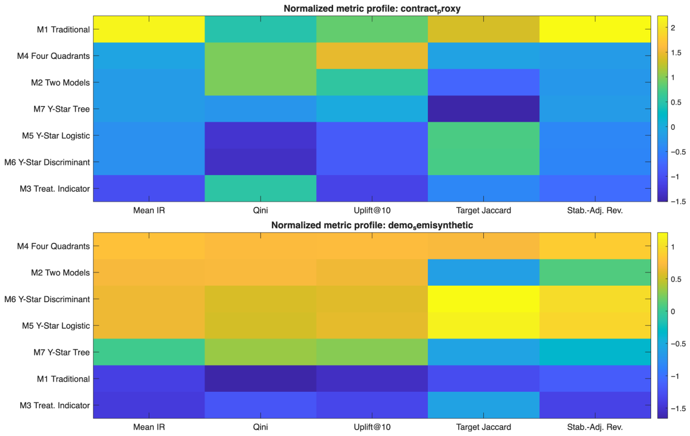
reports the scenario-wise averages used in the comparative analysis. Figure 1 complements Table 3 by providing a scenario-wise, standardized view of the main performance and stability dimensions. Each metric was z-scored within the scenario across model families, so the heatmap emphasizes relative rather than absolute differences. This representation visually demonstrates how the algorithmic profile of each model changes across both regimes.

In the panel representing the primary semisynthetic scenario, a clear visual cluster of high performance emerges across rows. Uplift-oriented algorithms robustly outperform traditional baselines. Model 4 achieves the highest mean incremental revenue (3706.0), followed by Model 2 (3517.4), Model 6 (3406.0), and Model 5 (3386.7). The ranking metrics mirror this ordering, as shown in the heatmap as dark intensity blocks spanning both the Qini and Uplift@10 columns. In contrast, the rows associated with the traditional baseline and treatment-indicator models show minimal intensity, reflecting their negative mean incremental revenue. Consequently, under a causally informative regime, optimization for causal uplift directly translates to maximizing financial returns.

This pattern drastically shifts in the contract-proxy scenario. Here, the intensity migrates almost entirely to the topmost row. Model 1 achieves by far the highest mean incremental revenue (28,180.0) and completely monopolizes the stability-adjusted revenue column, whereas all uplift-oriented families yield negative average yields. This visual inversion indicates that in the observational proxy regime, the dominant algorithmic signal remains the baseline response propensity rather than a recoverable treatment effect.

The heatmap also shows that ranking quality and economic utility can diverge under observational noise. Model 4 remains visually competitive in the Qini column, but its incremental revenue is negligible or negative. Thus, a model may rank customers by an apparent treatment divergence and still select a group that creates economic losses. This supports a key methodological caution: offline ranking curves should be complemented by checks on causal credibility and absolute economic value [4].

5.2. Stability of Targeted and Persuadable Sets

Table 4. Run-to-run stability of targeted and persuadable customer sets. Larger Jaccard and agreement values indicate more reproducible customer lists across random runs. Target Jaccard measures overlap in contacted customers, whereas persuadable Jaccard restricts the comparison to targeted customers with positive predicted uplift.

Model	Target Jaccard	Persuadable Jaccard	Target Agreement
Panel A: Semisynthetic causal
Model 6: Y-Star Discriminant	0.626	0.625	0.930
Model 5: Y-Star Logistic	0.613	0.611	0.927
Model 4: Four Quadrants	0.541	0.419	0.909
Model 7: Y-Star Tree	0.323	0.438	0.845
Model 3: Treatment Indicator	0.322	0.000	0.968
Model 2: Two Models	0.318	0.340	0.843
Model 1: Traditional	0.201	0.201	0.960
Panel B: Contract proxy
Model 1: Traditional	0.827	0.827	0.971
Model 5: Y-Star Logistic	0.690	0.662	0.982
Model 6: Y-Star Discriminant	0.685	0.682	0.981
Model 4: Four Quadrants	0.496	1.000	0.953
Model 3: Treatment Indicator	0.424	0.003	0.919
Model 2: Two Models	0.349	0.634	0.954
Model 7: Y-Star Tree	0.182	0.229	0.954

Stability is computed pairwise within each scenario over the repeated runs, restricting each comparison to the intersection of the two run-specific test sets. Jaccard values refer to overlap on shared customer identities, while target agreement denotes the mean fraction of shared customers receiving the same targeting decision.

summarizes the algorithmic run-to-run stability of the candidate families.

In the semisynthetic scenario, Model 4 generates the strongest economic policy but is less stable than the smoother Y-Star logistic and discriminant variants. This difference is not a contradiction but a consequence of the score construction. Model 4 estimates four observed treatment–response cells and ranks customers through a contrast of the corresponding class probabilities. Hence, small run-specific changes in any of the four cell probabilities can move customers close to the top-f threshold in or out of the target set. Models 5 and 6 collapse the same four cells into the binary $Y^{★}$ target, increasing the effective information available to each class and producing a more regular decision boundary. They trade part of the raw economic yield for greater run-to-run reproducibility. Model 7 also uses the $Y^{★}$ transformation, but its tree-based boundary remains more sensitive to split instability.

The persuadable Jaccard of 1.000 reported for Model 4 in Panel B arises because, in the contract proxy regime, the signed uplift scores produced are negative for almost all targeted customers. As a result, the persuadable subset ${\mathcal{P}}_f\left(m\right)$ (Equation (5)) is either empty or contains an identical, near-degenerate cluster of customers across virtually every run pair. Under the convention that undefined Jaccard values are excluded from the pairwise average (Section 3.4), the reported value reflects only the non-degenerate pairs, converging to unity. This value signals a pathological regime rather than real targeting robustness, and should not be interpreted as evidence of superior stability for Model 4 in the proxy scenario.

5.3. Winning Frequency Under Validation-Based Uplift-Only Selection

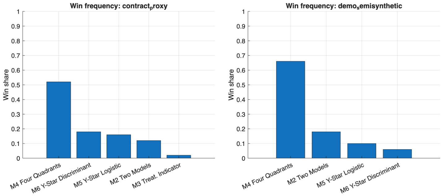
The repeated-run winner counts provide an additional perspective on model dominance (Figure 2). Here, a “winner” denotes the model selected at run level by the validation incremental-revenue criterion under the “uplift_only” selection scope. Accordingly, the win-frequency analysis summarizes competition among uplift-oriented models only.

In the primary semisynthetic scenario, Model 4 demonstrated robust superiority within the uplift-only competition, winning the majority of runs. This concentration of wins confirms that, when a treatment signal is present, the Four Quadrants architecture frequently provides the strongest validation-selected uplift policy among the candidate causal families.

In the contract proxy scenario, the distribution of winning uplift models becomes more fragmented. Model 4 still retains the largest share of uplift-only wins, but the dispersion across candidate winners increases notably, indicating a noisier and less stable competition landscape among uplift architectures. At the same time, Table 3 shows that the traditional baseline achieves the highest mean test incremental revenue in this regime. This is not a contradiction: the two summaries answer different questions, because Model 1 is excluded from the uplift-only winner selection by design. The contrast highlights a key deployment lesson: relative dominance within uplift models need not coincide with overall economic superiority on the test set.

5.4. Performance-Stability Trade-Off and Risk–Return Interpretation

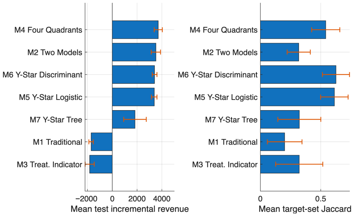
Figure 3 maps the performance–stability trade-off in the primary scenario. The results do not reveal a single universally dominant algorithm. Instead, they show a clear compromise: Model 4 maximizes mean test incremental revenue, whereas Models 5 and 6 achieve higher target-set Jaccard stability and lower across-run variability.

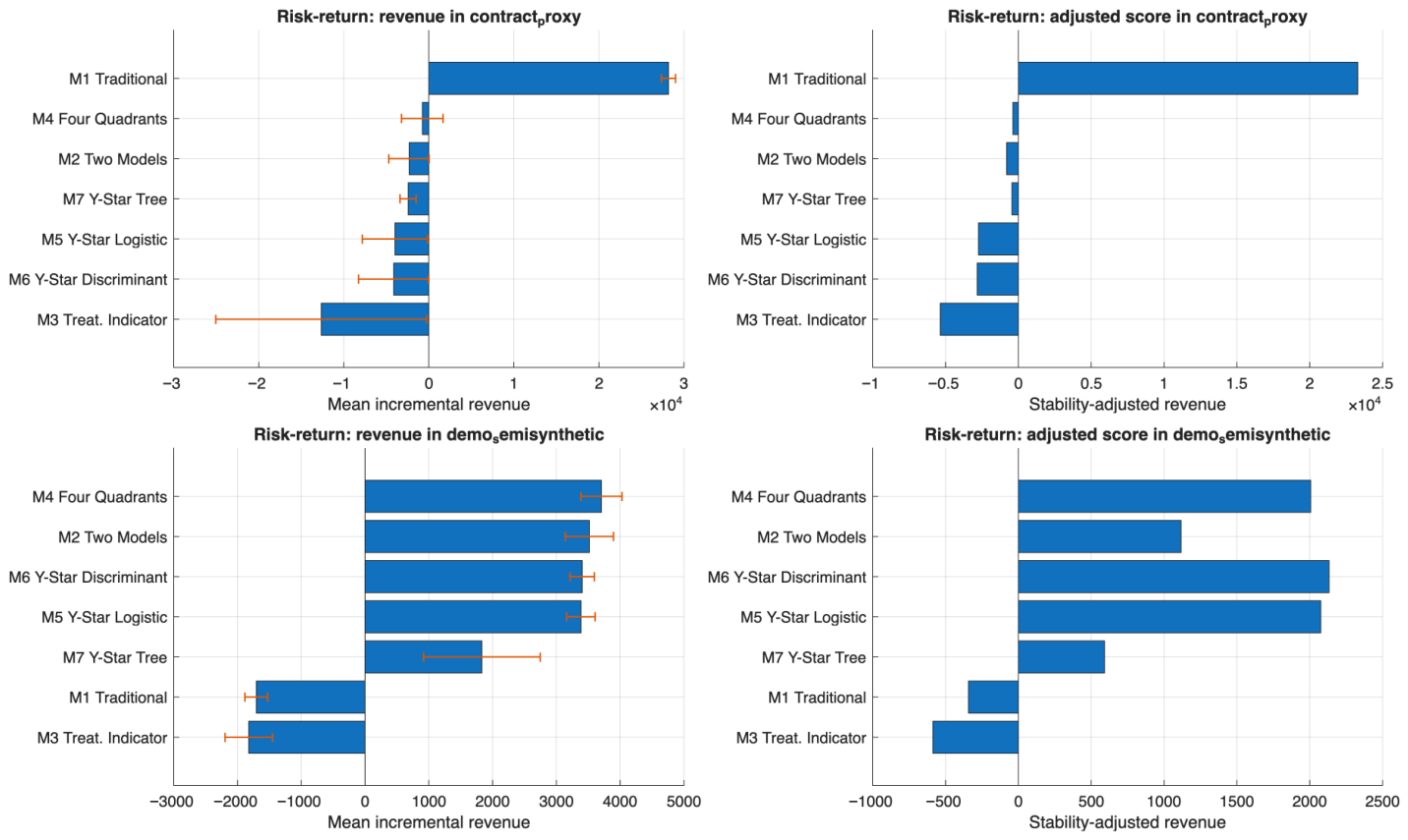
The operational consequences of this trade-off are summarized in the risk–return dashboard (Figure 4). The left panels report the mean test incremental revenue, whereas the right panels report the post hoc stability-adjusted revenue summary defined in Equation (27). This adjusted quantity is not used for model training or winner selection; rather, it provides an additional deployment-oriented lens that combines economic returns with targeting reproducibility.

In the semisynthetic regime, the dashboard revealed a rank reversal in the stability-adjusted summary. While Model 4 attains the highest mean test incremental revenue, Models 6 and 5 move ahead once target-set stability is incorporated. This does not alter the underlying validation-based winner-selection rule, but highlights that the most profitable policy in expectation need not be the most operationally reproducible.

In the observational proxy regime, the traditional baseline remains dominant in both the raw mean incremental revenue and stability-adjusted summary. This confirms that when the causal signal is weak or only partially corrected, a conventional response-oriented policy may offer a materially safer operational profile than noisier uplift architectures.

5.5. Policy Distillation and Interpretable Retention Segments

The final algorithmic step of the framework, which executes Algorithm 2, converts the opaque predictive scores of the winning policy into a globally interpretable rule set. A depth-bounded surrogate tree is fitted to a representative winning run from the primary scenario, selected from the modal winner class and chosen to be close to the median test’s incremental revenue within that class. The objective is interpretability rather than exact recovery: in the present experiment, the operational rule set depends on only three features, namely, fiber-optic Internet service, customer tenure, and electronic-check payment behavior.

As detailed in

Table 5. Distilled actionable segments for a representative winning run in the primary scenario, together with the corresponding empirical leaf-level uplift estimates.

Leaf Node	Rule	N	Share	Targeted N	Target Rate	Obs. Uplift
7	Fiber-optic Internet = yes Tenure $<34.5$ months Electronic check = yes	212	0.151	167	0.788	0.178
6	Fiber-optic Internet = yes Tenure $<34.5$ months Electronic check = no	132	0.094	36	0.273	−0.041
2	Fiber-optic Internet = no	781	0.555	0	0.000	−0.064
5	Fiber-optic Internet = yes Tenure $\ge 34.5$ months	283	0.201	8	0.028	−0.102

Leaf node denotes the internal identifier of the terminal CART node. The reported values refer to the terminal nodes actually present in the distilled surrogate tree, not to a consecutive numbering of leaves. Share denotes the fraction of the representative evaluation sample falling into the leaf. Targeted N and target rate refer to the customers selected by the original winning policy within each surrogate leaf. They indicate the local targeting intensity, and hence the descriptive fidelity, of the distilled segmentation. Obs. 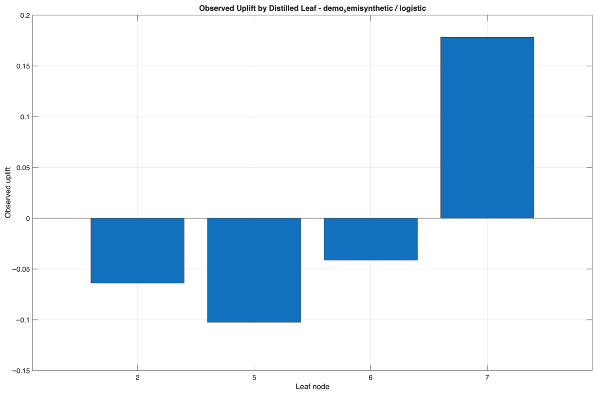uplift denotes the empirical treated-minus-control outcome difference observed within the representative winning run.

, Leaf 7 is the only leaf with a positive empirical uplift, capturing 15.1% of the representative evaluation sample and exhibiting an observed uplift of 0.178. In rule terms, this segment corresponds to customers with fiber-optic Internet service, tenure below 34.5 months, and electronic-check payment behavior. Within the representative run used for distillation, this is the only clearly treatment-sensitive subgroup isolated by the surrogate policy.

In contrast, Leaves 2, 5, and 6 exhibited a negative observed uplift in the same representative run. In uplift modeling, these leaves are consistent with non-persuadable or potentially sleeping-dog segments, namely, customer profiles for which intervention is ineffective or counterproductive. This result reinforces the value of selective targeting while remaining descriptive of the distilled run rather than a universal claim about the full population.

Figure 5 visually reinforces this. The contrast between the positive observed uplift in Leaf 7 and the negative uplift estimates in the remaining leaves highlights the importance of selective targeting in this study. A conventional response model could plausibly prioritize some of the negatively performing leaves because of their baseline risk profile, whereas the distilled uplift policy suggests that such interventions would not be value-enhancing in the representative run considered here.

Ultimately, this distillation step shifts the output from a black-box array of floating-point numbers to a deterministic, mutually exclusive set of marketing segments. The obtained rules are structurally comparable to the SATE-labeled strata produced in [6], but are generated via a post hoc surrogate that accommodates any upstream causal architecture, thereby operationalizing uplift modeling without sacrificing interpretability.

6. Discussion

6.1. When Uplift Modeling Adds Value

The results demonstrate that algorithmic uplift modeling adds significant value when the data-generating regime contains a sufficiently informative causal signal. In the primary semisynthetic scenario, uplift-oriented algorithmic families outperform the traditional baseline in both incremental revenue and uplift-specific ranking metrics (Table 3). This is the mathematical pattern expected when treatment effect heterogeneity is recoverable: policy selection is efficiently driven by the incremental treatment margin rather than by baseline retention propensity alone.

At the same time, the semisynthetic results revealed that maximizing the average predictive performance is insufficient on its own. While Model 4 is the strongest candidate in terms of mean incremental revenue and win frequency, Models 5 and 6 are more robust in terms of algorithmic stability and target-set overlap (Table 4, Figure 3).

6.2. Why the Traditional Model Dominates the Proxy Scenario

The contract proxy scenario provides complementary insights: uplift models do not automatically dominate observational datasets affected by selection bias. In this regime, the traditional supervised model remains economically dominant, whereas the uplift-oriented families return negative average incremental revenue (Table 3). The practical implication is direct: under the assumed value–cost calibration $(V,C)$, these uplift policies would spend more on contacted customers than they are expected to recover through incremental retention. They should not be deployed as full-scale campaigns without further validation. A firm facing this pattern should either retain the safer response-oriented baseline, reduce the target fraction, or run a randomized pilot with a no-contact holdout to obtain a cleaner treatment signal before relying on uplift-based targeting.

This interpretation follows from the design of the proxy scenario. Because the dataset lacks a randomized intervention, treatment is approximated through contract type. Although inverse propensity weighting partially mitigates observed selection bias in the economic evaluation, the setting remains observational and may still reflect baseline retention propensity more strongly than recoverable treatment heterogeneity. Therefore, the superiority of uplift modeling is conditional rather than universal: when a credible incremental-response signal is present, uplift policies can create value; when the signal is weak, confounded, or economically dominated by contact costs, a conventional response-oriented policy may be the safer operational choice.

6.3. Business Alignment and Stability as Joint Criteria

A central motivation of this study is that causal evaluation metrics and operational deployment objectives frequently diverge from each other. The empirical results confirm this. Across scenarios, the algorithm that performs best under one criterion does not necessarily perform best under another.

• In the semisynthetic regime, the policy that maximizes the mathematical expectation of revenue is notably unstable.
• In the proxy regime, the optimal “uplift-only” winner performs poorly in global economic terms.

Consequently, the proposed framework enforces a joint evaluation of the performance and stability. The operational question is not which architecture yields the largest AUQC but which algorithmic policy is simultaneously profitable, reproducible, and interpretable. Table 3 and Table 4, along with Figure 3 and Figure 4, demonstrate that these are mathematically distinct dimensions.

This distinction is critical from a deployment perspective because an operational system does not deploy a theoretical metric. Instead, it executes a targeting function and extracts a customer list. If the targeted subset shifts drastically across repeated runs, the policy loses its practical auditability. Therefore, in production systems, a slightly less profitable but more stable policy may be preferred.

6.4. Theoretical Implications

Theoretically, this study reframes uplift modeling as a deployment-oriented policy-selection problem rather than only as a CATE-ranking task. By combining incremental revenue, repeated-run target-set stability, and surrogate-rule interpretability, the framework extends standard uplift evaluation toward business-aligned causal decision support. This perspective clarifies why a model with strong Qini or AUQC performance may still be unsuitable for deployment if it generates unstable customer lists or negative economic value.

6.5. Practical Implications and Deployment Workflow for Targeted Campaigns

From a practical perspective, the framework translates uplift modeling into a concrete deployment workflow for deciding whether uplift-based targeting should be used, which model and target fraction should be selected, and which customer identifiers should enter the CRM campaign list.

First, the firm defines the eligible customer base E, the intervention to be evaluated (e.g., a discount, personalized retention call, or contract-upgrade incentive), the campaign budget, and the economic calibration $(V,C)$. A randomized pilot with a no-contact holdout group is the preferred data-collection design, because it provides the treated and control observations needed to estimate incremental response. If only historical non-randomized campaign data are available, the framework can still be used as an observational diagnostic, but the resulting targeting policy should be interpreted with the same caution discussed for the contract proxy regime.

Second, candidate policies are estimated on the development sample and the target fraction is selected on the validation set using the incremental-revenue criterion in Equation (20). Let $m^{★}$ denote the selected model and let $f^{★}=f_{m^{★}}^{★}$ denote its validation-selected target fraction. In a production campaign, each eligible customer receives a score $s_{m^{★}}\left(x_i\right)$ and the deployable target list is obtained by selecting the top-ranked customers:

$$A_E^{★}=\left\{i\in E:s_{m^{★}}\left(x_i\right)\ge q_{1-f^{★}}\left(\{s_{m^{★}}\left(x_j\right):j\in E\}\right)\right\},$$

(38)

where $q_{1-f^{★}}$ is the $(1-f^{★})$ empirical quantile of the scores in the eligible population. Thus, the targeted clients are the customer identifiers in $A_E^{★}$, whose size is approximately $\lceil f^{★}\left|E\right|\rceil$. Operationally, this means that the company does not contact the customers with the highest baseline churn risk, but the customers ranked highest by the selected incremental-response policy.

Third, the repeated-run stability layer is used as a pre-deployment diagnostic. This does not change the validation-based selection rule used in the experiments; rather, it informs the managerial decision of whether the selected customer list is sufficiently reproducible to be trusted in production. If two policies have comparable validation incremental revenue, the more stable policy may be preferred because it generates a more auditable and operationally consistent campaign list.

A practical deployment should also monitor data drift and cost sensitivity. Data drift occurs when customer features, churn behavior, treatment response, or campaign eligibility change after training. In a production CRM system, this can be monitored by comparing current and historical feature distributions, score distributions, treatment rates, and response rates. When drift is substantial, the firm should recalibrate the target fraction $f^{★}$, the uplift scores, and the surrogate rules. Cost sensitivity is also central because the selected policy depends on the business calibration $(V,C)$. If intervention cost increases, or if the value of a retained customer decreases, the break-even threshold $C/V$ rises and broader targeting may no longer be profitable. Before deployment, the firm should stress-test the selected policy under plausible value–cost scenarios.

Finally, the selected policy can be translated into business rules through the surrogate-tree distillation stage. The implementation produces two complementary deployment artifacts: a score-based CRM file containing customer identifiers, scores, and binary targeting decisions; and an interpretable segment description that explains which customer profiles are prioritized. In the empirical example, the positive-uplift segment identified in the representative run corresponds to fiber-optic customers with short tenure and electronic-check payment behavior, while leaves with negative observed uplift should not be prioritized. During live deployment, the firm should retain a small randomized holdout group to monitor realized incremental revenue, update the value-cost calibration, and periodically retrain the framework as customer behavior and campaign economics evolve.

6.6. Limitations and Future Work

The present study acknowledges several limitations that define the boundaries of the current empirical evidence and indicate directions for future research.

• The empirical validation relies on a single public dataset, namely the Telco Customer Churn dataset. Although this dataset is appropriate for illustrating retention-oriented targeting and enables a transparent repeated-run protocol, it represents only one industry, one customer population, and one feature space. Therefore, the reported performance and stability rankings should not be interpreted as universally generalizable across sectors. Future work should replicate the framework on additional datasets from different industries, campaign designs, and customer populations.
• This study does not validate the framework on a real randomized controlled trial. Instead, it relies on a causally controlled semisynthetic benchmark and on a propensity-weighted observational proxy. These regimes are useful for methodological comparison, but they cannot fully replace a randomized marketing experiment with a no-contact holdout group. As a result, the strongest causal claims remain confined to the semisynthetic setting, whereas the proxy regime should be interpreted as an observational stress test.
• The reported stability rankings are dataset- and regime-conditional. Although the repeated-run protocol provides evidence of reproducibility within the Telco Customer Churn setting considered here, it does not imply that the same algorithms would remain equally stable in another industry, with different client profiles, treatment mechanisms, outcome prevalence, or campaign economics. The proposed stability layer is intended as a diagnostic to be re-estimated in each new application rather than as a universal ranking of algorithmic robustness. Cross-industry validation on additional retention, marketing, and service-management datasets represents an important direction for future work.
• The present evaluation does not explicitly model temporal data drift or time-varying campaign economics. In real deployments, customer behavior, churn risk, treatment responsiveness, contact costs, and retention value may evolve over time. Future work should extend the framework with formal drift-detection diagnostics, periodic recalibration rules, and systematic sensitivity analyses over alternative $(V,C)$ configurations. This would allow the stability-aware selection layer to be combined with production monitoring tools that detect when a previously selected targeting policy should be retrained, revalidated, or replaced.
• The formulation is restricted to binary treatments. Future extensions should accommodate continuous treatment dosages, multi-armed treatment rules, and constrained optimization formulations via Integer Linear Programming [5,17], potentially incorporating fairness constraints to ensure equitable targeting across demographic subgroups.
• To isolate the effect of the uplift-modeling formulation, the main experimental design fixed the external base-learner setting to logistic regression for most model families, while retaining discriminant and shallow-tree variants only within the transformed-outcome family. This controlled design reduces hyperparameter-induced variability, but it may also limit predictive flexibility and external generalizability. Future studies should evaluate the same policy-selection layer with richer base learners, including gradient boosting, random forests, causal forests, generalized random forests, and neural uplift architectures.
• The targeting policy was discretized using a finite grid of candidate fractions, whereas continuous budget-constrained optimization could refine the final thresholds.
• The current architecture relies on standard tabular features. Extending this stability-aware framework to encompass multi-armed neural estimation architectures [26] and large-scale contextual embeddings [11] is a critical next step. In particular, the response-guided context grouping module in [11] provides a real architectural blueprint for mitigating distribution shifts when high-dimensional context features are present in the data.

7. Conclusions

This study presents a stability-aware, value-driven framework for customer-retention policy selection. It evaluates uplift modeling as a deployment-oriented decision problem. The assessment combines economic value, run-to-run stability, and rule interpretability, rather than relying only on offline treatment effect ranking metrics.

The empirical evidence supports three main conclusions. First, uplift-oriented algorithms add significant economic value when the underlying data-generating regime contains recoverable signals. In the primary semisynthetic scenario, uplift families outperform the traditional risk-response baseline in terms of both incremental revenue and causal ranking metrics (Table 3). Second, causal algorithms are not universally superior in all data environments. In the observational contract proxy scenario, the traditional supervised model remains economically dominant, indicating that confounded proxy settings are heavily driven by baseline response propensity rather than true treatment heterogeneity. Third, the repeated-run analysis demonstrates that the algorithm with the highest average mathematical expectation of revenue is not necessarily the most stable (Table 4, Figure 3 and Figure 4). Accordingly, causal policy selection should be evaluated based on both performance and stability rather than through a single-metric ranking exercise alone.

Another key contribution lies in the post hoc policy distillation stage. The framework translates complex predictive score arrays into compact Boolean decision rules via surrogate trees, isolating an actionable segment with a positive observed uplift in the representative winning run (Table 5 and Figure 5). The resulting rule structure, based on three features, (fiber-optic service, tenure, and payment method) is directly usable in standard CRM systems without requiring continuous numerical scores. This strengthens the practical viability of the methodology by translating the selected policy into transparent operational logic [6].

Overall, this study contributes a reproducible pipeline for selecting uplift policies, rather than a new causal estimator. The pipeline helps assess when uplift modeling is operationally useful, which model family offers adequate stability, and how the selected policy can be translated into interpretable CRM rules.