Diagnosis and Localization of Leaks in Industrial Compressed Air Systems Using the Dynamic Time Warping (DTW) Time Series Analysis Method

Abstract

Industrial pneumatic systems are central to automated production but often exhibit low efficiency and high energy costs due to pressure drops, leaks, and related issues. Air leaks increase operational expenses and degrade actuator performance. This study introduces a reliable classification-based approach for subsystem-level localization of single leaks. Each operating cycle is mapped to one of four actionable states using a Dynamic Time Warping (DTW) algorithm applied to time-series data from a single inlet flowmeter, distributor switching signals, and actuator end-position sensors. The method distinguishes whether a leak occurs in the supply line, actuator circuit, or dynamically during the extension stroke. Unlike conventional metrics such as Euclidean, Canberra, and Pearson distances, DTW does not require equal-length signals and compensates for leak-induced temporal shifts, achieving complete class separation. Experimental validation included 200 cycles: 50 under normal conditions and 150 across three fault states (inlet leak, actuator leak, and dynamic leak), sampled at 10 Hz. DTW distances showed no overlap between class distributions. A Leave-One-Out 1-NN classifier achieved 100% accuracy across all classes. The approach is low-cost, automated, and suitable for real-time implementation with minimal sensors, supporting integration into machine learning frameworks and enhancing energy efficiency in pneumatic systems.

1. Introduction

Industrial pneumatic systems are key infrastructure in any automated industrial production, powering over 70% of automated processes. Different studies show that industrial enterprises use between 5 and 40% of the electricity consumed to produce compressed air [1,2], in some more specialized industries, this share reaches 50% [3].

1.1. Relevance of the Problem

Pneumatic systems are a universal means of automation, characterized by safety and reliability even in aggressive or explosive environments. However, they suffer from extremely low energy efficiency [4]. Various studies show, for example, that energy costs represent over 75% of the total costs, including investment, over the entire life cycle of an industrial compressor [5]. The study [6] states that the specific productivity of compressed air systems is in the order of 0.15 kWh/m³, which makes this energy medium extremely expensive from an energy point of view. Despite the high cost of compressed air, a significant amount of it is wasted without performing any work. Industry data shows that between 20% and 40%, and in some poorly maintained installations up to 60%, of the compressed air produced in factories is wasted, mainly due to leaks in end-user components, faulty fittings, worn seals and improperly maintained components [7]. In an experimental study of a real industrial system, the repair of 77 identified leaks (totalling 2.82 m³/min or ~20% of capacity) resulted in a saving of 447 kWh per day, corresponding to a reduction in CO₂ emissions of about 63.5 tons per year [2].

It is characteristic of leaks that they occur constantly due to ageing of materials, mechanical vibrations, thermal deformations, etc., which means that a well-maintained pneumatic system must also be well monitored.

The problem has three main dimensions:

-

Energy losses and direct cost: A leak with a diameter of 1 mm at a pressure of about 7 bar can lose hundreds of litres of compressed air per minute, which equates to thousands of euros in annual loss [8]. Separately, leaks cause pressure drops in the system, which forces compressors to operate at a higher load to compensate for these drops, which shortens their service life [9].

-

Environmental impact: Excess electricity used to compensate for leakage losses means additional carbon emissions. In the context of global initiatives for sustainable development and the transition to a “green” industry, reducing these emissions is a top priority for industrial enterprises. There is already a recognized need to implement measures to reduce CAS losses and minimize the carbon footprint associated with these systems [10].

-

Operational stability: In pneumatic systems, to be precise and efficient, it is necessary to maintain a relatively stable pressure. Leaks lead to pressure drops that can disrupt the synchronization of pneumatic actuator cycles and lead to production inefficiency or defective output [11,12].

1.2. Brief Overview of Existing Methods for Leaks Detection (Acoustic, Ultrasonic, Pressure/Flow-Based, Machine Learning)

The problem of leaks in pneumatic systems is systemic and is well known to all manufacturing enterprises. Because of this, many methods have been developed over time to detect, locate and size leaks. They can be summarized in several main categories:

Ultrasonic and acoustic methods

These are the best known and most common approaches to solving the problem. They are based on the fact that when pressurized air passes through a small opening it generates turbulence and sound waves in the ultrasonic spectrum (20–40 kHz) [13]. Ultrasonic detectors are quite well developed and improved over time and can accurately locate the leak that generated the ultrasound under certain conditions. Some recent research demonstrates a method of Distributed Acoustic Sensing, which allows for real-time detection of problems [14]. For hard-to-reach areas, additional analysis of the acoustic characteristics is used [15].

Infrared thermography

Due to the Joule–Thomson effect, when compressed air expands during a leak (air decompression), a sharp drop in temperature is observed at the leak point. Infrared cameras, often integrated with computer vision algorithms, are used to detect such anomalies. Such an approach also allows for automatic detection and relatively accurate localization of leaks [16,17].

Machine vision-based methods

In [18] a method for identifying anomalies in the movement of the pneumatic actuator using a non-contact machine vision system is demonstrated. The proposed scheme consists of three sets of labels: one for the actuator position, one for monitoring the operation of the limit switches and one for monitoring the switching of the PLC. A camera is used to monitor these marks and evaluate the performance of the actuator. The authors assume that monitoring exactly this set of marks can be used to detect anomalies in the movement, including those due to leaks.

Another approach, also using machine vision, has been applied in two studies [19,20], in which diagnostics of possible leaks in a pneumatic valve are performed by observing the movement of the pneumatic actuators. By comparing the captured image with the data from the controlling PLC, the percentage of opening of the piston rod and, accordingly, the deviations from its normal position are determined. In this way, a possible leak in the valve can be identified. Pressure drops at the inlet valve, again caused by a leak, can also be identified—with reduced pressure in it, deviations in the piston rod displacement of up to 85% have been recorded, which shows that this method can be used to detect leaks in the valve and in front of it.

Machine Learning-Based Methods

Increasingly, IIoT sensors generate vast amounts of data, mostly time series. Machine learning involves various algorithms for analyzing this data. These algorithms can gather knowledge about the normal state of increasingly complex systems and analyze and identify anomalies. Hybrid ensemble learning has been successfully applied, providing predictive models for identifying individual leaks [21,22]. For machine learning to be complete and effective, appropriate algorithms must be found to classify existing anomalies in systems, which also provide insight into these causes. Statistical and time series processing methods are often used for this [23]. The study presented in [24] compares different methods for the classification of single leaks, based on time series of air flow in a single pneumatic cell. Different Minkowski distances, as well as methods for correlation analysis such as Pearson, are investigated. The authors conclude that for sufficiently reliable identification and differentiation of different leaks, it is necessary to use a hybrid method—a combination of Canberra distance and Pearson correlation analysis.

A detailed study of the application of machine learning methods is presented in the publication [25]. Pressure data and flow data are combined using the so-called exergy flow rate of compressed air.

In [26], classification algorithms for detecting leaks in the forward and reverse strokes of a cylinder are synthesized. In forming a feature space, a wavelet transform is used and applied to the time trend of the flow during one cycle of the pneumatic cylinder.

In [27], the operation of the laboratory pneumatic system is diagnosed as a whole, using the flow time series obtained from a flowmeter at the system inlet. The feature space is formed by a set of mathematical-heuristic features and coefficients from the fast Fourier transform. The synthesized diagnostic classifier is trained on time trends (images) of normal operation (one-class classifier with nearest neighbour data description technique).

DTW-Based Fault Diagnostics in Fluid and Mechanical Systems

Although Dynamic Time Warping (DTW) diagnostics were originally developed for speech recognition, they are increasingly employed in the diagnostics of industrial mechanical and fluid systems due to their inherent ability to handle temporal distortions under varying operating conditions.

In fluid systems, DTW-based methods are used to classify events deviating from normal states by analyzing their similarity to historical time-series data from baseline operations. For instance, ref. [28] proposes a model for leak detection and localization in gas pipelines based on Variational Mode Decomposition and Dynamic Time Warping (VMD-DTW). Experimental results demonstrate that the proposed DTW method can reliably identify waveform distortions induced by leaks, even under noisy conditions, achieving superior denoising performance and higher localization accuracy.

In [29], DTW is utilized to compare observed and simulated behaviours of a multi-layered water distribution system for leak detection. The localization process employs a multi-graph approach that combines sensor data and network topology to determine the sensor coverage area. The Dynamic Time Warping algorithm calculates the similarity between observed and simulated data, thereby identifying probable leak locations. The results demonstrate the effectiveness of this methodology, as it detects anomalies within 15 min of leak onset and localizes them within 50 m of the actual leak site.

Despite these advances, pneumatic fault diagnosis has largely focused on cycle-time monitoring, thresholding, or machine-learning classifiers rather than explicit temporal alignment of transient flow signatures. Consequently, DTW has not, to the authors’ knowledge, been systematically applied to multi-class leak localization in pneumatic actuator systems using only upstream flow data. This gap is significant because pneumatic leak signatures are strongly influenced by valve timing, actuator stroke variability, and pressure-wave propagation delays—conditions under which DTW may provide substantial advantages over static feature extraction or threshold-based methods by preserving temporal fault morphology while compensating for operational variability.

1.3. Limitations of Traditional Approaches

Limitations of Acoustic and Ultrasonic Methods

Although this is the most common method in the industry because it can be used without stopping production and without the need for additional complex sensor networks and analysis of huge databases, this method has quite serious disadvantages. It is extremely time-consuming and dependent on the experience and skills of the operator [30]. The diagnostic devices used in these methods are highly sensitive to ambient background noise (from machinery, acoustic reflections, air flows), which often leads to false positive signals, incorrect sizing of leaks, and even missing leaks with relatively small flow rates [31,32]. The effectiveness of this method for identifying leaks drops sharply with increasing distance between the detector and the object, and when estimating the size of the leak, the average error reaches 75% for holes with a diameter of more than 1.5 mm [33]. As a result of all this, this method does not work reliably in large and difficult-to-access networks of pneumatic elements, or in the presence of air flows that create a “blind spot” [34]. These disadvantages make ultrasonic and acoustic methods unsuitable for continuous monitoring and automatic leak localization.

Limitations of Infrared Thermography

These methods require more sophisticated optical equipment and direct visibility to the monitored systems, which makes their use quite limited. This is especially true for leaks hidden in panels and boxes or thermally insulated parts of the pneumatic system [35,36]. At distances of 1 m and more, small leaks, under 1 mm become difficult to see and practically indistinguishable, especially with strong ambient reflections. Only larger holes—over 2 mm—give a clear signal with good enough contrast to be accurately localized—Refs. [17,37]—which, like ultrasound methods, makes this method unsuitable for real-time monitoring.

Limitations of machine vision-based methods and standard machine learning algorithms

Although machine learning, pattern recognition, and deep supervised learning are promised for development in the field of leak diagnostics and localization, they require a lot of labelled data [38], which is difficult to achieve in compressed air system diagnostics due to their complexity and amorphous nature. In the case of inhomogeneous data with noise, as well as in the case of amorphous changes to the systems (new users, replaced elements with insufficiently close analogues, seasonality of the load, etc.), the models suffer from overfitting and poor generalizability to changed conditions [39]. In [40] and other reviews, it is pointed out that these methods face data scarcity, high labelling costs, and sensitivity to noise, and even well-designed models are difficult to adapt to different pneumatic configurations. Additionally, the complexity of the sensor network and the relative slowness in processing huge amounts of data makes these methods still difficult to adopt by the industry [41].

1.4. Industrially Applicable Solutions to the Problem

The search for improvements in this sector has led to products that offer autonomous monitoring and error control capabilities in a single package, examples of which are the ‘Energy Efficiency Module’ of FESTO [42], “Air Management System” of SMC [43] and “Smart Pneumatics Monitor” of AVENTICS PNEUMATICS [44].

Their systems use sensor data to identify leaks. In fact, all of them use flow and pressure data, with the latter also using cycle time characteristics. In terms of control capabilities, the “Smart Pneumatics Monitor” system offers greater functionality. It is claimed that automatic pressure maintenance, via proportional pressure regulators, reduces the increase in compressed air consumption due to leaks. Working towards addressing this problem is the “Automatic Leak Detection System” concept from SMC [45]. The system is based on sequential testing of each actuator of the machine in a special test mode and can identify the presence of a leak in the supply line, distributor, and actuator, as well as measure its size. This information narrows the search for the leak and helps the maintenance personnel decide on the best time for subsequent search and elimination.

Despite the availability of commercial platforms, given the complexity of the task arising from the presence of pneumatic systems with multiple components and actuators, multiple potential leak points and multiple physical relationships between compressed air parameters, the leak identification task continues to be a subject of research interest. Research continues in several directions—development of sensor technologies, data processing and analysis, use of intelligent methods to increase the accuracy of detection and localization, adaptability of the developed systems, visualization of information, including in cloud spaces, etc.

Unlike commercial solutions, which rely on offline testing in a dedicated machine test mode, the proposed method can be applied during normal production operations. Furthermore, the proposed method does not require additional hardware, as it utilizes data from standard sensors already available within a conventional IIoT/PLC system. This study addresses the problem at the level of a simplified system with a single actuator (similar to commercial systems); however, this is only an initial step toward expanding to multi-actuator systems. Such an expansion is explicitly planned in Section 5 and aligns with established research practices in comparable studies within the field [25,41].

1.5. Novelty of the Proposed Solution

In this study, we propose an approach for classification of single leaks in a basic pneumatic system based on DTW analysis of time-series data of compressed air flow measured at the system inlet. The core novelty lies in the systematic exploitation of DTW’s inherent invariance to nonlinear time shifts and variable cycle lengths. In real pneumatic systems, leaks cause both amplitude changes in flow rate and significant temporal distortions—cycle-length variations up to 15–20% and time lags due to pressure drops and additional air consumption. Unlike traditional lock-step metrics (Euclidean, Minkowski, Canberra), which require time series of identical length and penalize displacements along the time axis, DTW operates directly on variable-length cycles and is therefore insensitive to the time shifts that leaks inevitably produce. This property is particularly valuable in inertial and nonlinear systems such as pneumatics, and contrasts directly with the hybrid Canberra–Pearson approach required in our previous study [24].

By applying DTW, each operating cycle is mapped to one of three actionable fault classes—static leak at the supply line, static leak at the actuator circuit, or dynamic leak—enabling subsystem-level localization that directly guides maintenance personnel to the affected area. Because the DTW distance alone serves as the classification feature, no labelled fault data are required beyond the initial no-leak calibration phase. The method is directly integrable into lightweight machine-learning classifiers within existing IIoT/PLC infrastructures, offering a calibration-light, real-time alternative to commercial platforms that rely on sequential offline testing and multi-point instrumentation.

This paper presents a proof-of-concept validation on a single-actuator pneumatic circuit. This scope is intentional; it establishes the DTW classification baseline under controlled conditions before extension to multi-actuator systems, which is the subject of ongoing work within the ERDF project BG16RFPR002-1.014-0005.

2. Materials and Methods

2.1. Description of Laboratory Compressed Air System

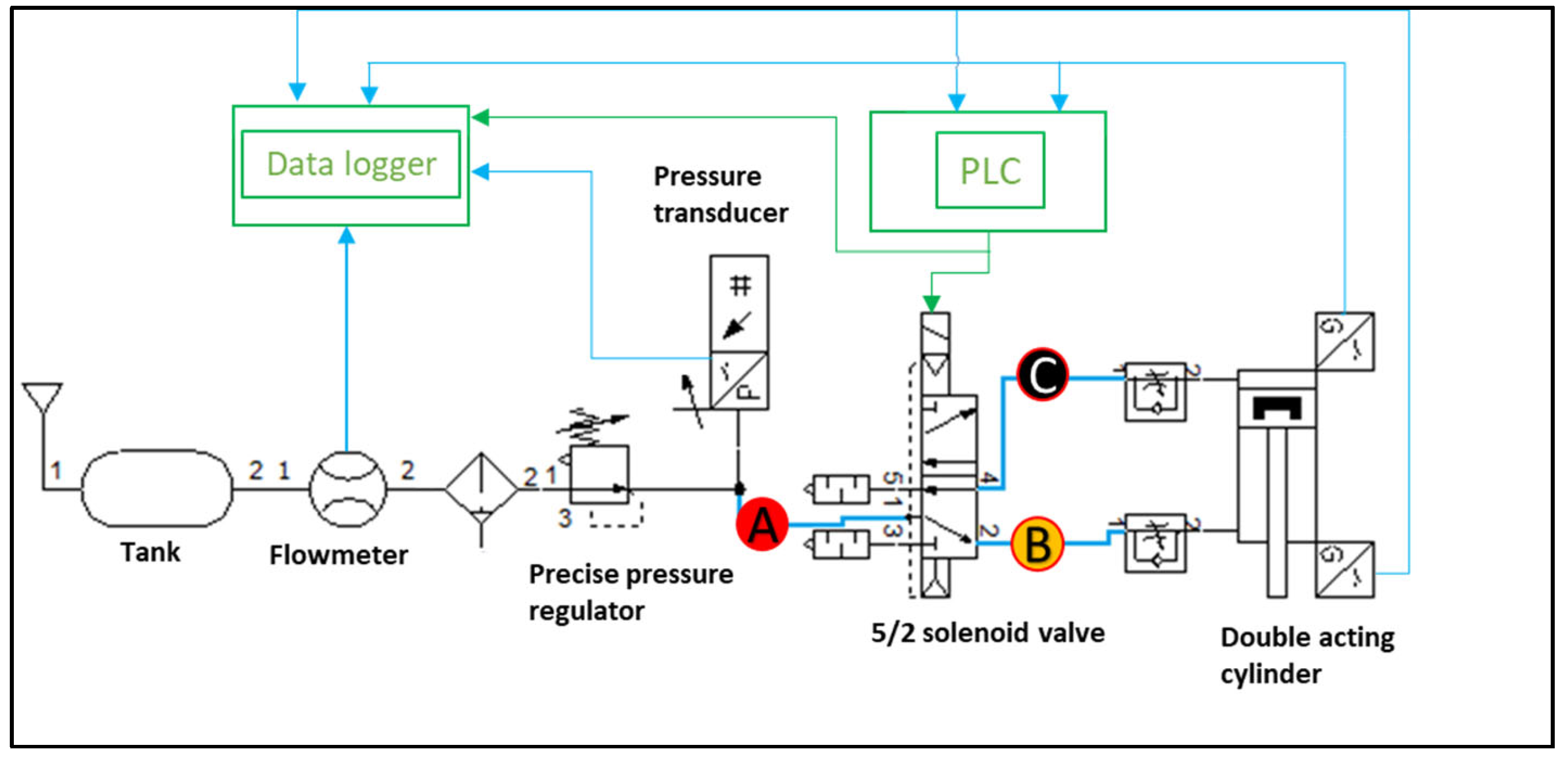
For the purposes of the study, a laboratory test model of a simple pneumatic circuit was implemented (see Figure 1).

The elements used in the test bench are standard industrial elements. The specification of the elements can be seen in

Table 1. Pneumatic elements for the test bench.

Name	Manufacturer	Part Number	Description
Tank	FESTO, Esslingen am Neckar, Germany	CRVZS-10	Air tank 10 L, 2.0 MPa
Flowmeter	SMC, Tokyo, Japan	PFM710-C6-F-N	Digital Flow Switch without Monitor, 0.2–10 L/min
Filter	FESTO, Esslingen am Neckar, Germany	MS2-LF-QS6	Air Filter
Precision regulator	FESTO, Esslingen am Neckar, Germany	LRP-1/4-0.7	Precision regulator
Pressure transducer	FESTO, Esslingen am Neckar, Germany	SPAU-P10R-G18FD-L-PNLK-PNVBA-M8U	Digital pressure switch
5/2 Valve	FESTO, Esslingen am Neckar, Germany	VUVG-L10-M52-RT-M5-1P3	5/2 Solenoid Valve
Double acting cylinder	FESTO, Esslingen am Neckar, Germany	DSNU-20-125-P-A	Round Cylinder
Speed regulators	FESTO, Esslingen am Neckar, Germany	GRLA-1/8-QS-4-D	Speed Controller (G1/8-4 mm)
End-position sensors	FESTO, Esslingen am Neckar, Germany	SMT-8M-A-PS-24V-E-0,5-M8D	Magnetic proximity sensor.

.

2.2. Theoretical Basis for Dynamic Time Warping (DTW)

Dynamic Time Warping (DTW) is a well-known algorithm for finding and measuring the similarity between two time series with possible differences in length and/or temporal offsets. The time series are warped in a nonlinear manner to match each other as closely as possible. In areas such as data and information extraction and analysis, DTW performs successfully and is therefore widely applied in automatically dealing with time warps and different speeds [46]. Unlike classical distance metrics (e.g., Euclidean), DTW compensates for local stretches and contractions along the time axis, making it particularly suitable for studying flow profiles in pneumatic systems, where leaks cause both amplitude changes and cycle delays [47].

Let the two time series being compared be the test series $Q=\left(q_1,q_2\dots q_n\right)$ and reference series $C=(c_1,c_2\dots c_m)$.

For each pair of members in both series $\left(q_i, c_j\right)$ the difference $\delta \left(i,j\right)$ is calculated by the square of the difference ${\left(q_i- c_j\right)}^2$, the absolute value of the difference $\left|q_i- c_j\right|$ or other suitable distance or measure.

In this work, the local cost is defined using the squared Euclidean distance between scalar samples in order to increase sensitivity to larger deviations, which are expected for different leaks sizes. The algorithm starts by constructing the local distance (cost) matrix:

$$\delta \left(i,j\right)={(q_i-c_j)}^2$$

(1)

On this basis, the accumulated distance matrix is recursively computed as:

$$D\left(i,j\right)=\delta \left(i,j\right)+\mathrm{m}\mathrm{i}\mathrm{n}\left\{D\left(i-1,j\right), D\left(i,j-1\right), D(i-1,j-1)\right\}$$

(2)

with initial conditions: $D\left(\mathrm{0,0}\right)=0;D\left(i,0\right)=D\left(0,j\right)=+\mathrm{\infty }.$

The optimal warping path $W={\left\{\left(i_k,j_k\right)\right\}}_{k=1}^K$ represents the minimum-cost path through the accumulated distance matrix D.

When searching for a solution using the dynamic programming approach, the following constraints are imposed on the points $W_k=(i_k,j_k)$ of the time warping path [48]:

• Boundary conditions—the path must start from point $W_1=\left(\mathrm{1,1}\right)$ and end at point $W_K=(n, m)$, i.e., the first and last terms of the two time series must match. From the perspective of the cumulative difference matrix, the path must start from the lower left corner and end in the upper right corner.
• Continuity conditions—the increments between successive path points are restricted to, at most, one in each coordinate direction (${0<i}_k-i_{k-1}\le 1$ and $0<j_k-j_{k-1}\le 1$). This guarantees a locally continuous alignment path without skipping elements in the time series.
• Monotonicity condition—the points must be monotonically ordered in time, such that $i_{k-1} \le i_k$ and $j_{k-1} \le j_k$. Therefore, the time warp path only goes forward, without going back in time.
• Slope constraint condition—the path should be neither too steep nor too gentle, i.e., there should not be many consecutive increases in only one of the coordinates of the points on the path. Otherwise, there will be long sequences of members of one time series, connected to one member or a small number of consecutive members of the other series.
• Band constraint condition—the path should not deviate significantly from the main diagonal of the cumulative difference matrix. The points on the path should fall within the time wrapping window, of width r ($\left|i_k-j_k\right|\le r$). It sets the permissible distance in time of the connected members of the two time series [49]. Without constraint, DTW has quadratic computational complexity $O\left(\mathrm{n}\mathrm{m}\right)$, where n and m are the lengths of the two time series. To reduce the computational complexity to practically linear and prevent unrealistic deformations, the Sakoe-Chiba band constraint with width $r = 10\%$ of the length of the longer series is applied. This limits the search for an optimal path to only a band around the main diagonal and guarantees real-time execution at industrial sampling rates.

The DTW distance between the two series is the value in the last cell:

$$DTW\left(Q,C\right)=D(n,m)$$

(3)

2.3. Classification Workflow

Reference series construction performed (once prior to deployment).

During an initial calibration phase (50 cycles used in this study), cycles recorded under confirmed no-leaks conditions are averaged point-wise to produce the reference series C (see Section 2.2).

Online classification phase (executed per cycle)

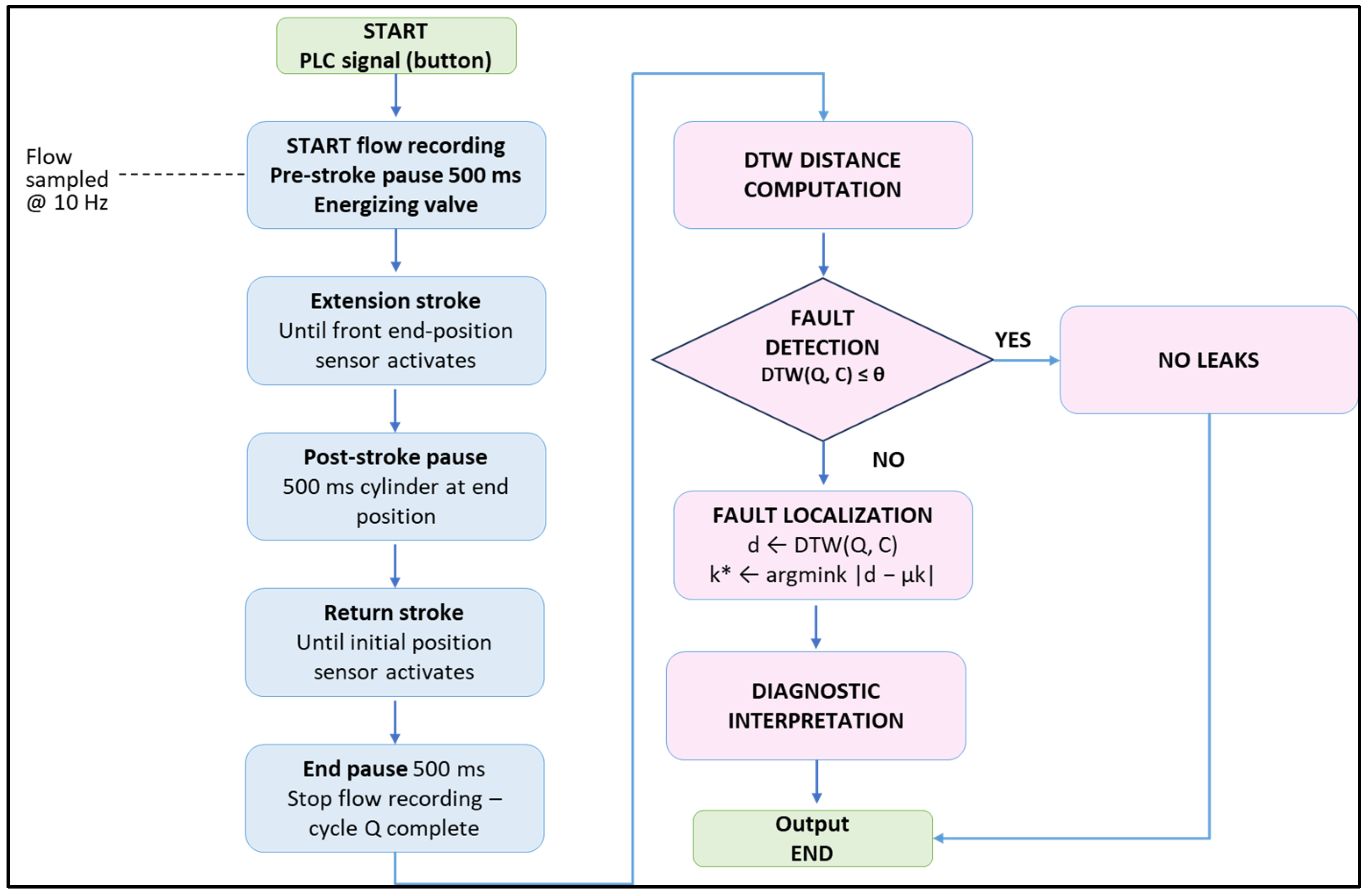
Step 1—Cycle segmentation. The cycle in the laboratory experiment begins with a signal to the controller, which after 500 ms switches the valve and continues for 500 ms after the cylinder returns to its normal state. Each cycle contains: the 500 ms pre-stroke pause, the extension stroke (until the front end-position sensor activates), the 500 ms post-stroke pause, and the return stroke (until the rear end-position sensor activates) and 500 ms end pause.

Step 2—DTW distance computation. For each new cycle $\mathit{Q}$ (of arbitrary length), the DTW distance $\mathit{D}\mathit{T}\mathit{W}\left(\mathit{Q},\mathit{C}\right)$ is computed using the squared Euclidean local distance measure and the Sakoe-Chiba band constraint $\mathit{r}=\mathbf{10}\mathit{\%}$ of $\mathit{m}\mathit{a}\mathit{x}\left(\left|\mathit{Q}\right|,\left|\mathit{C}\right|\right)$, as defined in Equations (1)–(3).

Step 3—Fault detection. If $\mathit{D}\mathit{T}\mathit{W}\left(\mathit{Q},\mathit{C}\right)\le \mathit{\theta }$ (threshold $\mathit{\theta }$ = 9.1, defined as the $\mathbf{3}\mathit{\sigma }$ upper bound of the no-leak distribution), the cycle is classified as normal. Otherwise, a fault is flagged.

Step 4—Fault localisation. The fault class is assigned by nearest-centroid rule: the cycle is assigned to the class $\mathit{k}\in \{\mathit{S}\mathit{t}\mathit{a}\mathit{t}\mathit{i}\mathit{c} \mathit{S}\mathit{u}\mathit{p}\mathit{p}\mathit{l}\mathit{y}, \mathit{S}\mathit{t}\mathit{a}\mathit{t}\mathit{i}\mathit{c} \mathit{A}\mathit{c}\mathit{t}\mathit{u}\mathit{a}\mathit{t}\mathit{o}\mathit{r}, \mathit{D}\mathit{y}\mathit{n}\mathit{a}\mathit{m}\mathit{i}\mathit{c}\}$ whose mean DTW distance ${\mathit{\mu }}_{\mathit{k}}$ is closest to $\mathit{D}\mathit{T}\mathit{W}(\mathit{Q},\mathit{C})$.

The workflow described above is formalized in Algorithm 1. The four steps map directly onto the two phases of the system: Steps 1 and 2 constitute the signal acquisition and distance computation pipeline. Steps 3 and 4 implement the two-stage diagnostic decision—first determining whether a fault exists, then identifying its class. The complete cycle structure is illustrated in Figure 2.

Algorithm 1. DTW-Based Leak Detection and Localization.

Input • Q—inlet flow time series (one operating cycle sampled at 10 Hz) • C̄—reference series obtained as the mean of 50 confirmed no-leak cycles • θ = 9.1—fault detection threshold (3σ upper bound of no-leak distribution) • μSupply = 49.87, μActuator = 28.1, μDynamic = 19.07 Output Diagnostic state ∈ {Normal, Static-Supply, Static-Actuator, Dynamic} Step 1—Cycle Segmentation 1. Wait for PLC trigger signal 2. Start recording flow at 10 Hz 3. Record pre-stroke pause (500 ms) 4. Record extension stroke until front end-sensor activation 5. Record post-stroke pause (500 ms) 6. Record return stroke until rear end-sensor activation 7. Record end pause (500 ms) 8. Stop recording flow 9. Set Q ← full-cycle flow signal Step 2—DTW Distance Computation 1. Set r ← 0.1 × max(|Q|, |C̄|)//Sakoe–Chiba band width 2. For each (i, j) such that |i − j| ≤ r: 3. δ(i, j) ← (qi − c̄j)2//local squared Euclidean cost 4. D(i, j) ← δ(i, j) + min{D(i − 1,j), D(i,j − 1), D(i − 1,j − 1)} 5. Compute DTW(Q, C̄) ← D(|Q|, |C̄|)//accumulated cost Step 3—Fault Detection 1. If DTW(Q, C̄) ≤ θ 2. Return: Normal//false alarm rate < 0.3% 3. Else proceed to Step 4 Step 4—Fault Localization 1. Set d ← DTW(Q, C̄) 2. Compute k* ← argmink |d − μk| 3. Return k* ∈ {Static-Supply, Static-Actuator, Dynamic}

3. Results

3.1. Description of the Experimental Setup and Generated Scenarios

The conducted experiment includes 200 measurements of operating cycles, of which there are 50 measurements in the reference configuration (without leaks) and 50 measurements for each of three different situations of real leaks. Leaks are divided into two main categories:

-

Static leaks—leaks, with high consumption, as they are either in the main lines or at the machine level in standby mode. In the first case, the losses are constant, in the other they are during the machine downtime and when the actuator is in the starting position.

-

Dynamic leaks, which are observed in the actuators or more precisely in the distributor-fittings-hoses-actuator system. When the system is in the initial state (for example, the cylinder is with the rod retracted), these leaks are not observed. After switching the system (the cylinder is with the rod extended), a leak appears. Usually this is a leak from worn actuator or distributor seals, but often it is also from a defective fitting or connection that is under pressure only in this position of the system.

In the laboratory model, in accordance with Figure 1, the following three configurations are implemented sequentially and separately:

-

node A: static leak in the supply part of the system—before the distributor, including the supply port of the distributor;

-

node B: static leak in the actuator part (cylinder part)—between the distributor and the cylinder, including leak in the distributor and leak in the cylinder front seal;

-

node C: dynamic leak—between the distributor and the cylinder in the line for the straight stroke of the cylinder, including leak in the distributor itself when switching it to this state.

The diameter of the leak-generating orifice was fixed and calibrated at 1 mm for all three configurations, which, at a pressure of 5 bar, results in a leak rate in the range of 0.9–1.2 L/min. This level of leak is of medium severity according to data from numerous real-world industrial audits [7,13]. As expected, the influence of the leak size on the DTW distance is monotonic, as larger leaks lead to greater amplitude and temporal deviations, which DTW reflects as proportionally larger distances. A similar dependency is observed in [24], where various Minkowski distances respond in a scaled manner depending on the size of the leak. The systematic investigation of various scenarios, including variations in leak size, has been identified as a direction for future work (Section 5).

Each operating cycle is defined as described in Section 2.3 (Step 1) and comprises five phases: pre-stroke pause, extension stroke, post-stroke pause, return stroke, and end pause. Data recorded per cycle include the actuator end-position sensor states, the distributor switching signal, and the inlet flow values, sampled at 10 Hz (every 100 ms).

For convenience, the system inlet pressure is fixed (5 bar) by means of a precise regulator and using a sufficiently large tank.

3.2. Graphical Representation of Time Series and DTW Matrices

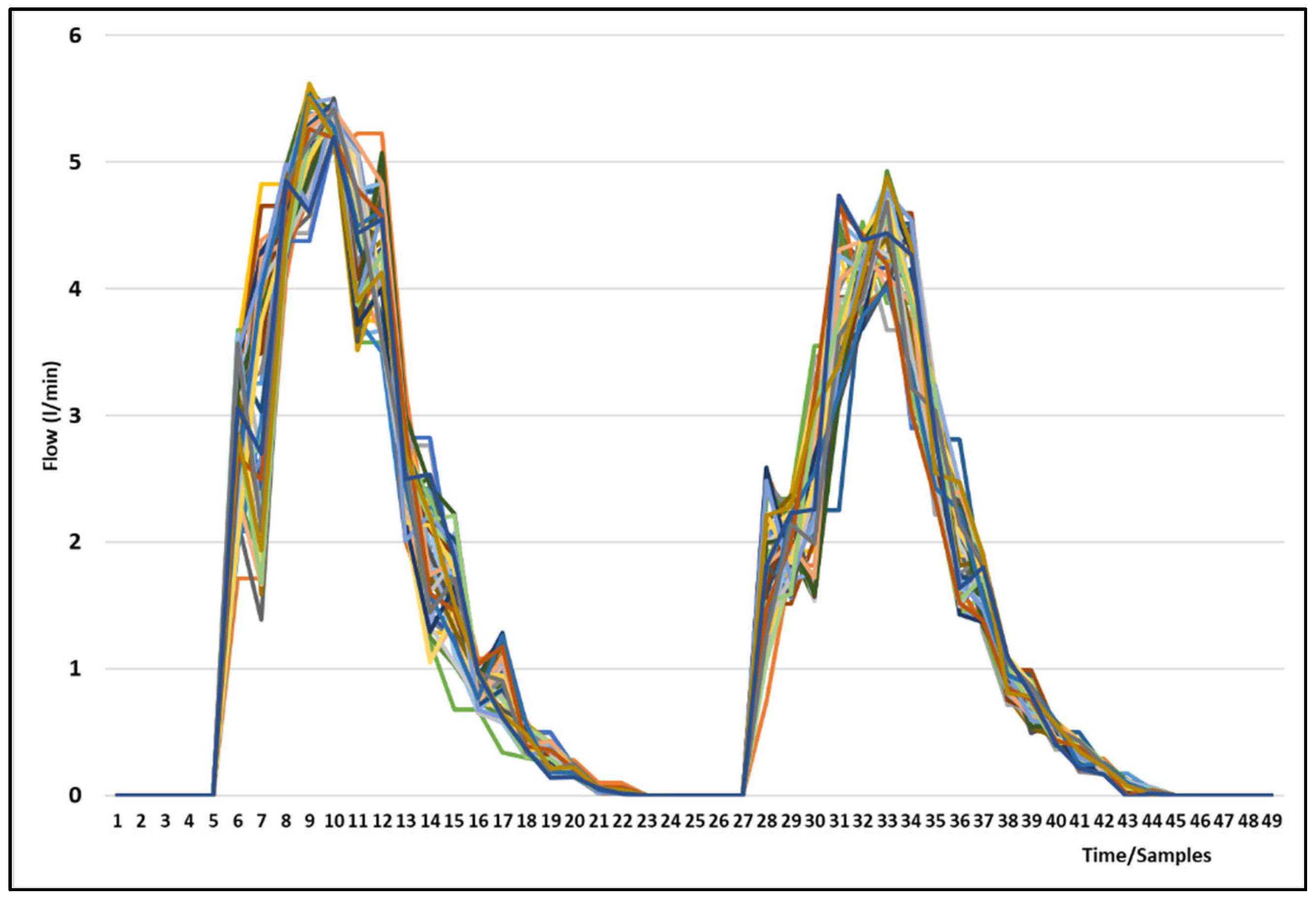
Figure 3 shows the family of time series of measurements taken in the no-leak situation.

Visual analysis of the time diagrams, in the “no leak” situation, shows:

-

The presence of stationary and random variations in the supply pressure values. In this case, the pressure at the inlet of the system is fixed by a mechanical pressure regulator with flow compensation. The stationary variations are the result of pressure drops in the supply line.

-

All 50 cycles exhibit identical length, reflecting stable actuator kinematics under fixed supply pressure. Direct point-by-point averaging was therefore applied without prior alignment to construct the reference series.

-

Local variations are possible in certain segments of the process as a result of clearances, friction, etc.

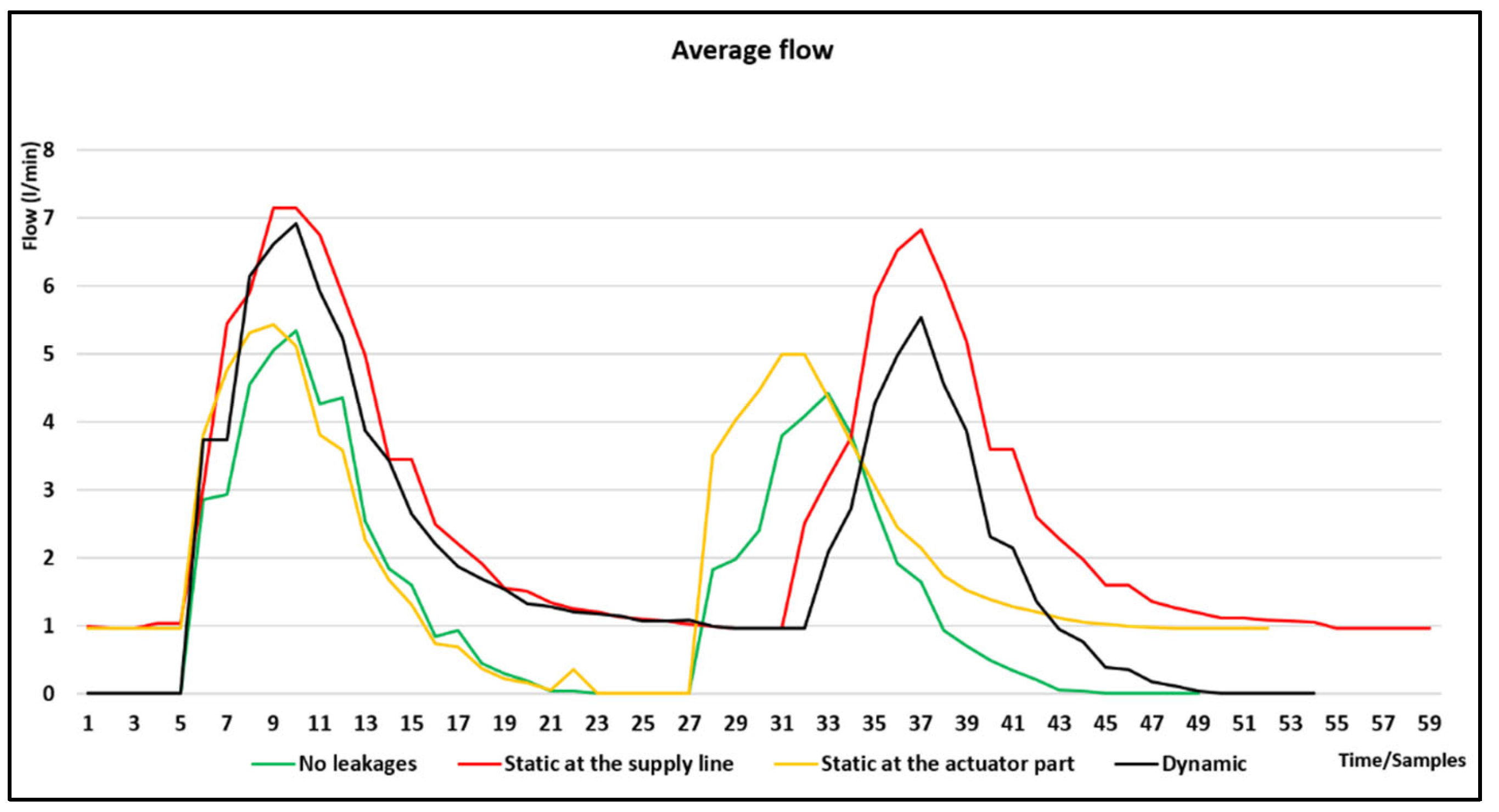
Figure 4 shows the time series of the average values in the four states of the system. The time shifts from the normal state caused by the occurrence of leaks are very clearly visible.

For the compiled sample of experimental data, a quantitative analysis of the observed quantities was performed against the averaged values of the measurements during normal (no leaks) operation.

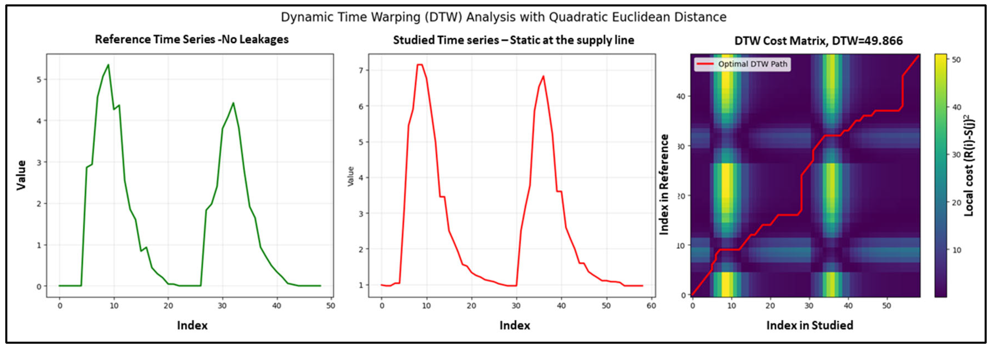
Figure 5 shows the diagrams of the results of the DTW calculations between the averaged values of the measurements during normal (no leaks) conditions and the averaged values at “static leak” at the supply line.

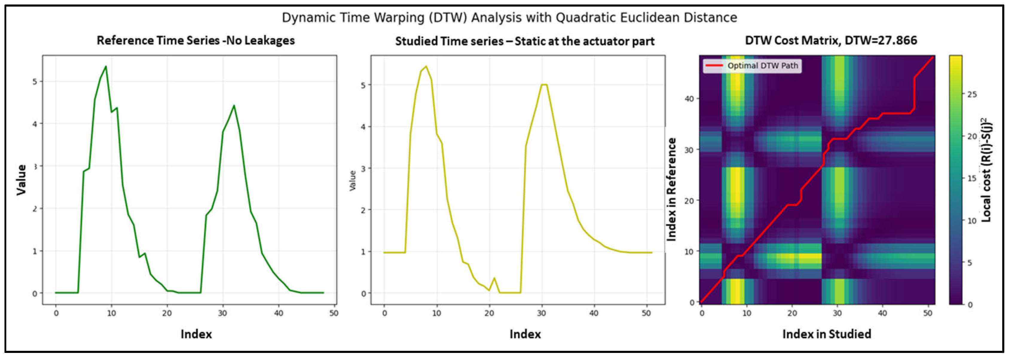
Figure 6 shows the diagrams of the results of the DTW calculations between the averaged values of the measurements during normal (no leaks) conditions and the averaged values “static leak” at the actuator part.

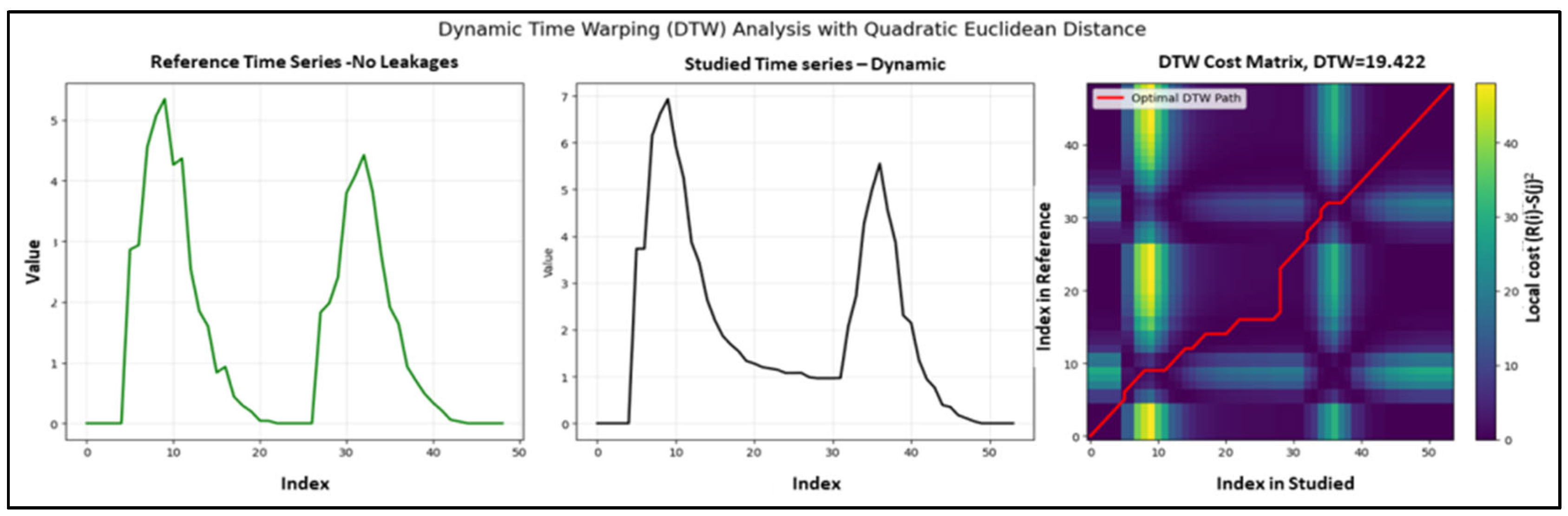
Figure 7 shows the diagrams of the results of the DTW calculations between the averaged values of the measurements during normal (no leaks) conditions and the averaged values at “dynamic leak”.

The figures on the right illustrate a typical DTW result—represented through a weighted grid-based coordinate system and an optimal warping path. The application of DTW under the “multiple objects to a single reference” principle implies the construction of an averaged time series, which is defined as a reference (template). In many DTW applications, the similarity between time series data can be visually assessed through the plotted graph. In the case of a perfect match, the optimal path is a straight line

For each group of measurements—50 measurements for each group, No Leaks, Static at Supply line, Static at the actuator part and Dynamic—DTW comparisons were made with the average values of No Leaks.

3.3. Statistical Analysis and Classification Performance of DTW Results

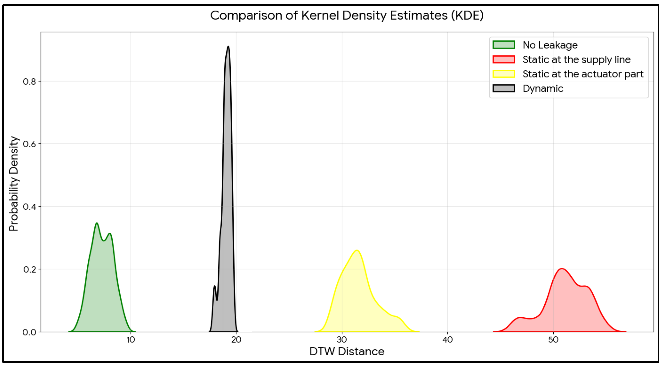
To further examine the distribution of DTW distances within each system state, a Kernel Density Estimation (KDE) was applied to the four groups of 50 measurements. KDE provides a smooth, continuous estimate of the underlying probability density function without assuming a predefined distributional form, making it a more informative visualization than discrete histograms for sample sizes of this scale. The resulting distributions are presented in Figure 8. The bandwidth for every single state is calculated regarding Scott’s rule as follows:

No Leaks—$h=0.4653$

Static at the supply line—$h=0.9450$

Static at the actuator part—$h=0.7499$

Dynamic—$h=0.1858$

Figure 8. Kernel Density Estimation (KDE).

Figure 8. Kernel Density Estimation (KDE).

The normality of each distribution was verified using the Shapiro–Wilk test ($\alpha = 0.05$). Results are presented in

Table 2. Results of Shapiro–Wilk test ($\alpha = 0.05$).

Column/Series Name	W-Statistic	p-Value	Normally Distributed?
No Leaks	0.9669	0.1751	Yes
Static at the supply line	0.9634	0.1264	Yes
Static at the actuator part	0.9575	0.0718	Yes
Dynamic	0.9602	0.0945	Yes

.

Since the p-value for every single series is greater than 0.05, we fail to reject the null hypothesis. This confirms that the data in all four categories follows a normal distribution.

The results of performing ANOVA Test are: $F\left(3196\right)=8447.53$, $p<0.001$.

The differences between the four states are extremely significant.

The four states are clearly distinguishable via the DTW distance parameter. The Dynamic group shows the highest stability (lowest standard deviation), while Static at the supply line exhibits the highest variance (dispersion).

To provide additional formal classification performance metrics, a 1-Nearest Neighbour (1-NN) classifier was applied using Leave-One-Out Cross-Validation (LOOCV).

Since the input data consists of 1D scalar distances—each cycle is represented by a single DTW distance value computed against the reference series—the distance metric between any two points simplifies to the absolute difference between them. This makes the 1-NN LOOCV evaluation both computationally trivial and fully transparent. The results (

Table 3. Classification performance metrics.

Metric	Value
Accuracy	1.0000
Precision (Macro)	1.0000
Recall (Macro)	1.0000
F1 Score (Macro)	1.0000

and

Table 4. Confusion matrix.

Actual\Predicted	No Leaks	Dynamic Leak	Static Actuator Leak	Static Supply Leak
No Leaks	50	0	0	0
Dynamic	0	50	0	0
Static at actuator part	0	0	50	0
Static at supply line	0	0	0	50

) confirm that the four states are perfectly separable based on the DTW distance parameter.

3.4. Comparative Performance of DTW Versus Classical Distance Metrics

To make the advantage of using DTW in this case objectively clear, we will compare the results with our earlier study [24], which employed classical lock-step distance and similarity measures for time-series analysis, including Euclidean distance, Manhattan, Canberra distance, Pearson correlation and Angular separation. A fundamental limitation of these classical methods is that they are lock-step (point-wise) distances and therefore require time series of identical length. As shown in Figure 4, leaks introduce substantial cycle-length variations and time lags caused by additional air consumption and the resulting pressure drops. As shown in [24], additional pre-processing of the data is required to use these methods. For this purpose, we have chosen linear interpolation (compress), since padding (adding 0 to the shorter series) distorts the Canberra distance a lot, which is very sensitive to values close to 0, and trimming can exclude data useful for the analysis.

The results are summarized in

Table 5. Statistical summary of distance/correlation values (mean ± standard deviation) for the four system states (200-cycle dataset, 50 replicates per class).

Metric	No Leaks	Static Supply Leak	Static Actuator Leak	Dynamic Leak
DTW (proposed, Sakoe-Chiba, r = 10%)	7.29 ± 0.6	49.87 ± 1	28.1 ± 0.8	19.07 ± 0.5
Euclidean (after sync)	1.98 ± 0.31	10.87 ± 0.34	7.64 ± 0.4	6.88 ± 0.42
Manhattan (after sync)	7.82 ± 1.19	71.68 ± 2.00	41.25 ± 2.13	35.53 ± 2.2
Canberra (after sync)	3.28 ± 0.63	29.33 ± 0.23	18.78 ± 0.53	13.75 ± 0.33
Pearson dissimilarity (1 − corr., after sync)	0.975 ± 0.008	0.974 ± 0.007	0.921 ± 0.017	0.939 ± 0.010
Angular separation (after sync)	0.992 ± 0.003	0.965 ± 0.002	0.955 ± 0.009	0.966 ± 0.006

.

The DTW distances in the three faulty situations (49.87 ± 1.0 Static at the supply line, 28.1 ± 0.8 Static at the actuator part and 19.07 ± 0.5 Dynamic leak) are significantly larger than the corresponding values of Euclidean distance and Canberra distance and are comparable in scale to Manhattan. In addition, all methods used in [24] for time series analysis show partial or significant overlap in different classes. The only exception is Canberra distance, but there the relative separation is also smaller.

Pearson correlation and Angular separation values are on a different scale (similarity measures), but they also show significant overlapping in different classes of leaks.

This direct comparison of the same data set confirms that DTW overcomes a fundamental limitation of classical metrics in pneumatic systems: their sensitivity to nonlinear time distortions caused by leaks.

The superior class separation achieved by DTW directly supports reliable classification-based localization, delivering actionable subsystem-level guidance that lock-step metrics cannot provide without significant preprocessing and loss of diagnostic information.

4. Discussion

4.1. Interpretation of the Results

The experimental results clearly demonstrate that the DTW between the reference time series (No Leaks) and the series with leaks allows a reliable distinction between the four system states. The visual analysis of Figure 4 shows time shifts and amplitude changes in the averaged profiles for the three types of leaks. These shifts are due to the additional air consumption and pressure drops, which increase the time to reach the end positions of the cylinder and changes the cycle speed. The quantitative evaluation by DTW (Figure 5, Figure 6 and Figure 7) confirms that the minimum distances are significantly higher for all leaks compared to the reference state. Kernel Density Estimation of DTW values for 50 measurements in each group (Figure 8), validated by the Shapiro–Wilk test, confirms that each category follows a normal distribution and shows strong separability with no overlap between distributions.

The classification of DTW distance (Table 5) is not arbitrary; it reflects the physical location of each leak.

A static supply line leak persists throughout the entire cycle, resulting in continuous air loss. This leads to the highest consumption and the longest cycle duration, which explains the large DTW distance (49.87 ± 1).

Static actuator circuit leak occurs when the cylinder is in its home position and is inactive during the forward stroke. The resulting distance is lower (28.1 ± 0.8).

Dynamic leak is activated only during the cylinder’s forward movement and its dwell time in the end position, disappearing during the return stroke and the stay in the initial position. In this scenario, the DTW distance is the smallest (19.07 ± 0.5) but still forms a clearly distinct class.

Compared to other metrics reported in [24], DTW does not require data pre-processing or synchronization and handles variations in cycle length across different states very effectively (up to 15–20%, as shown in Figure 4). From a diagnostic perspective, the proposed method enables narrowing the search space from the entire pneumatic system to a specific subsystem.

For instance, a DTW distance above approximately 9.1—representing the $3\sigma$ upper bound of the “No-Leaks” distribution (7.29 + 3 × 0.60)—indicates the presence of a fault condition with a false-alarm rate below 0.3%. Once a fault is confirmed, the magnitude of the DTW distance directly determines the subsystem likely affected:

DTW~17–21: Indicates dynamic leak, which may be caused by a defective cylinder or distributor seal, or a damaged push-in fitting or connecting tube.

DTW~26–30: Indicates static leak in the actuator circuit (fittings, hoses, or the front cylinder seal).

DTW > 47: Indicates static leak in the supply line upstream of the distributor.

This method—relying on a single scalar distance value and requiring neither additional sensors nor dedicated offline test modes—differs fundamentally from commercial systems, which can only confirm the presence and approximate magnitude of a leak but require the system to operate in a dedicated test mode to classify the affected subsystem.

4.2. Advantages of DTW

The main advantage of DTW is its robustness to nonlinear time deformations and local delays, which are typical for pneumatic systems due to the compressibility of air, the inertia of actuators and pressure variations. Unlike conventional lock-step metrics such as Minkowski or Canberra distances, DTW compensates for displacements along the time axis and compensates for both amplitude and phase differences. This allows reliable classification even at variable cycle rates (variations in the length of the series up to 15–20%). The method does not require a large volume of labelled data—one reference series of the normal state obtained during a calibration phase is sufficient. This eliminates the main drawback of classical ML approaches and makes the method directly applicable in real industrial conditions. By applying the Sakoe-Chiba band (r = 10%), the computational complexity is reduced to practically linear, enabling computationally efficient execution suitable for real-time operation at a sampling rate of 10 Hz.

4.3. Limitations and Possible Improvements

The experiments were conducted with a fixed leak-generating orifice, identical across all three configurations, representing an equivalent level of severity. It is expected that Dynamic Time Warping (DTW) will scale monotonically as the leak size changes. Validation at different levels and under inlet pressure fluctuations remains an open question and is the focus of future research.

Additional idealized conditions include:

(1) Fixed supply pressure—real networks exhibit ±0.5–1.5 bar fluctuations that may shift the no-leaks reference distribution;

(2) Single-actuator circuit—multi-actuator systems produce superimposed flow signatures requiring more advanced segmentation;

(3) Controlled low-noise laboratory environment—industrial electromagnetic interference and mechanical vibration may affect flow signal quality at 10 Hz;

(4) Fixed 10 Hz sampling rate—fast-cycling systems may require higher sampling or adaptive segmentation.

Furthermore, in the case of simultaneous multiple leaks (not investigated in the present experiment), the warping path may become more complicated and may reduce classification performance.

Possible improvements:

-

Hybrid combination with lightweight machine learning classifiers (e.g., k-NN or Random Forest on DTW distances as a metric) for automatic classification;

-

Adaptive updating of the reference series through continuous learning when a “normal” state is confirmed (e.g., after the installation of a new pneumatic component);

-

Real-time integration via edge computing—DTW is calculated in parallel for each completed cycle and compared to a threshold determined by the statistics of the normal distribution. This would allow immediate alarming and localization without stopping production;

-

Possibility of graphical interpretation of results.

5. Conclusions

This research shows that the analysis of time series of compressed air flow by Dynamic Time Warping is an effective and reliable method for diagnosing and locating single leaks in a pneumatic circuit. By using a single flowmeter and a discrete signal for switching the solenoid valve, a clear distinction of a reference state from three types of leaks (static in the supply part, static in the actuator part and dynamic) is achieved. DTW successfully compensates for time deformations and amplitude variations that classical metrics fail to handle. Experimental results obtained from 200 measurements sampled at 10 Hz confirm the statistical significance of the method and show clear separation between all classes without overlap.

The proposed method enables subsystem-level localization by identifying the specific leakage region (the supply line, the section between the directional control valve and the cylinder, or a dynamic leak occurring during the cylinder forward stroke). This level of diagnostic resolution is sufficient to localize the fault within the corresponding subsystem and support subsequent corrective actions.

The method offers a low-cost, automated solution for continuous monitoring that can reduce energy losses and increase the operational stability of production lines. It is compatible with existing IIoT infrastructures and can be integrated into modern predictive maintenance systems, reducing the dependence on manual inspections and expensive specialized devices.

Future research should focus on:

-

Testing the method in complex systems with multiple actuators and simultaneous leaks;

-

Developing an online version of DTW calculations with adaptive update of the reference profile, updating, and validating the approach under real industrial conditions (automotive and food industry) with variable loads and background noise;

-

Hybrid models combining DTW distances with lightweight neural networks to predict the evolution of leaks over time;

-

Implementation in a local pneumatic system based on PLC and HMI;

-

In real industrial environments, reference cycles may exhibit cycle-length variation due to supply pressure fluctuations or mechanical wear. In such cases, DTW Barycenter Averaging (DBA) is identified as the appropriate method for reference series construction and is planned as a direction for future work.

The next validation phase, already scheduled within the European Regional Development Fund project BG16RFPR002-1.014-0005, will include a multi-actuator test rig and an industrial pilot installation. These activities will strengthen the method’s readiness for full-scale deployment in production environments.

Pursuing these directions will enable full automation of diagnostics and will contribute to more sustainable and energy-efficient pneumatic system use.

References

1. Kosturkov, R.; Nachev, V.; Titova, T. System Analysis and Opportunities for Optimization of Pneumatic Systems in Manufacturing Plants. TEM J. 2019, 8, 749–763. [Google Scholar] [CrossRef] [Scilit]
2. Zaim, A. Industrial Compressed Air System Optimization: Experimental Evaluation of Energy Efficiency and Sustainability Gains. Processes 2025, 13, 3590. [Google Scholar] [CrossRef] [Scilit]
3. Borg, M.; Refalo, P. Failure Detection Techniques on the Demand Side of Smart and Sustainable Compressed Air Systems: A Systematic Review. Energies 2023, 16, 3188. [Google Scholar] [CrossRef] [Scilit]
4. Rogovyi, A.; Romasevych, Y.; Stryzha, M.; Kryvobok, R.; Krutikov, G.; Iglin, S. Transient Energy Conversion and Compressed Air Recovery in Pneumatic Systems: Optimization and CFD-Based Analysis. Actuators 2026, 15, 135. [Google Scholar] [CrossRef] [Scilit]
5. Vyas, V.; Jeon, H.-w.; Wang, C. An Integrated Energy Simulation Model of a Compressed Air System for Sustainable Manufacturing: A Time-Discretized Approach. Sustainability 2021, 13, 10340. [Google Scholar] [CrossRef] [Scilit]
6. Titova, T.; Kosturkov, R. Metaheuristic Method of Decision Making Based on an Expert Analysis of Leakage Losses in Pneumatic Systems. TEM J. 2026, 15, 18–26. [Google Scholar] [CrossRef] [Scilit]
7. Nascimento, G.F.M.; Wurtz, F.; Kyo-Peng, P.; Delinchant, B.; Batistela, N.J. Quantifying Compressed Air Leakage through Non-Intrusive Load Monitoring Techniques in the Context of Energy Audits. Energies 2022, 15, 3213. [Google Scholar] [CrossRef] [Scilit]
8. Blaustein, E.; Radgen, P. Compressed Air Systems in the European Union; LOG_X Verlag GmbH: Stuttgart, Germany, 2001. [Google Scholar]
9. Schmidt, C.; Kissock, K. Power Characteristics of Industrial Air Compressors; University of Dayton: Dayton, OH, USA, 2003. [Google Scholar]
10. European Environment Agency. Greenhouse Gas Emission Intensity of Electricity Generation in Europe; European Environment Agency: Brussels, Belgium, 2024. [Google Scholar]
11. Dindorf, R.; Takosoglu, J.; Wos, P. Review of Compressed Air Receiver Tanks for Improved Energy Efficiency of Various Pneumatic Systems. Energies 2023, 16, 4153. [Google Scholar] [CrossRef] [Scilit]
12. Zhu, H.; Wang, Z.; Wang, H.; Zhao, Z.; Xiong, W. Leakage Fault Diagnosis of Two Parallel Cylinders in Pneumatic System with a Minimal Number of Sensors. Electronics 2023, 12, 3261. [Google Scholar] [CrossRef] [Scilit]
13. Kosturkov, R.; Nachev, V.; Titova, T. Expert estimation of leakage in the pneumatic systems in the bottling industry. In IOP Conference Series: Materials Science and Engineering Plovdiv; IOP Publishing: Bristol, UK, 2020. [Google Scholar]
14. Benabid, M.-K.; Baumgartner, P.; Jin, G.; Fan, Y. Leakage Detection Using Distributed Acoustic Sensing in Gas Pipelines. Sensors 2025, 25, 4937. [Google Scholar] [CrossRef] [Scilit]
15. Yang, Y.-P.; Chu, S.-L.; Jing, Y.-H.; Sun, B.-C.; Zhang, J.-W.; Wang, J.-Y.; Fan, J.-C.; Li, M.-S.; Liang, M.-S.S.; Zheng, Y.-S. Experimental Study on Simulated Acoustic Characteristics of Downhole Tubing Leakage. Processes 2025, 13, 1586. [Google Scholar] [CrossRef] [Scilit]
16. Tong, K.; Wang, Z.; Si, L.; Tan, C.; Peiyang, L. A Novel Pipeline Leak Recognition Method of Mine Air Compressor Based on Infrared Thermal Image Using IFA and SVM. Appl. Sci. 2020, 10, 5991. [Google Scholar] [CrossRef] [Scilit]
17. Semitela, Â.; Silva, J.; Girão, A.F.; Verdasca, S.; Futre, R.; Lau, N.; Santos, J.P.; Completo, A. Combining Infrared Thermography with Computer Vision Towards Automatic Detection and Localization of Air Leaks. Sensors 2025, 25, 3272. [Google Scholar] [CrossRef] [Scilit] [PubMed]
18. Jura, J.; Kubica, J.; Cejnek, M.; Kuchar, M. Fault Diagnosis in Manufacturing Systems Using Machine Vision. In Proceedings of the 23rd International Conference on Process Control (PC), Strbske Pleso, Slovakia, 1–4 June 2021. [Google Scholar] [CrossRef] [Scilit]
19. Santhosh, K.V.; Shenoy, V.; Navada, B.R. Fault identification and isolation in pneumatic valve using image Processing. In Proceedings of the 2016 IEEE Distributed Computing, VLSI, Electrical Circuits and Robotics (DISCOVER), Mangalore, India, 13–14 August 2016. [Google Scholar] [CrossRef] [Scilit]
20. Loska, A.; Macha, A. The method of detecting leaks in pneumatic actuators on the example of a selected production system. TIAM—Technol. I Autom. Montażu 2025, 127, 62–73. [Google Scholar] [CrossRef] [Scilit]
21. Liu, T.; Cai, X.; Zhou, W.; Wang, K.; Wang, J. Enhanced Detection of Pipeline Leaks Based on Generalized Likelihood Ratio with Ensemble Learning. Processes 2025, 13, 558. [Google Scholar] [CrossRef] [Scilit]
22. Wu, H.; Jiang, Z.; Zhan, X.; Cheng, J. Research on a Novel Unsupervised-Learning-Based Pipeline Leak Detection Method Based on Temporal Kolmogorov–Arnold Network with Autoencoder Integration. Sensors 2025, 25, 384. [Google Scholar] [CrossRef] [Scilit]
23. Dobossy, B.; Formánek, M.; Stastny, P.; Spáčil, T. Fault Detection and Identification on Pneumatic Production Machine. In Proceedings of the Modelling and Simulation for Autonomous Systems: 8th International Conference, Virtual, 13–14 October 2021. [Google Scholar] [CrossRef] [Scilit]
24. Kosturkov, R.; Titova, T.; Nachev, V. Diagnosis of Pneumatic Systems on Basis of Time Series and Generalized Feature for Comparison with Standards for Normal Working Condition. TEM J. 2021, 10, 183–191. [Google Scholar] [CrossRef] [Scilit]
25. Zhang, C.; Wang, Z.; Yu, L.; Zhao, Z.; Wang, F.; Xiong, W. Leakage Detection in Pneumatic Systems with Machine Learning and Upstream Single-Point Signals. Int. J. Fluid Power 2025, 26, 1–24. [Google Scholar] [CrossRef] [Scilit]
26. Zhang, K. Fault Detection and Diagnosis for Multi-Actuator Pneumatic Systems. Ph.D. Thesis, Stony Brook University, Stony Brook, NY, USA, 2011; p. 975. [Google Scholar]
27. Ertel, W.; Lehmann, R.; Medow, R.; Finkbeiner, M.; Meyer, A. Model Free Diagnosis of Pneumatic Systems using Machine Learning. In Proceedings of the 9th International Fluid Power Conference, Aachen, Germany, 24–26 March 2014. [Google Scholar]
28. Wang, Y.; Wenzhuo, L.; Zhang, Q.; Feng, L.; Liu, W. Gas pipeline leakage detection and localization method based on VMD-DTW. Flow Meas. Instrum. 2025, 102, 102820. [Google Scholar] [CrossRef] [Scilit]
29. Barros, D.; Zanfe, A.; Menapace, A.; Meirelles, G.; Herrera, M.; Brentan, B.M. Leak detection and localization in water distribution systems via multilayer networks. Water Res. X 2025, 26, 100280. [Google Scholar] [CrossRef] [Scilit]
30. Gong, Y.; Bao, C.; He, Z.; Jian, Y.; Wang, X.; Huang, H.; Song, X. A Review on Gas Pipeline Leak Detection: Acoustic-Based, OGI-Based, and Multimodal Fusion Methods. Information 2025, 16, 731. [Google Scholar] [CrossRef] [Scilit]
31. Ota, Y.; Nukaga, S.; Kanda, Y.; Furuya, M. Explainable Machine Learning for Bubble Leakage Detection at Tube Array Surfaces in Pool. Appl. Sci. 2025, 15, 12587. [Google Scholar] [CrossRef] [Scilit]
32. Zeng, J.; Cai, B. Real-Time Detection of Small Liquid Drip in Pipeline in Complex Industrial Scenes Based on Machine Vision. Appl. Sci. 2026, 16, 2823. [Google Scholar] [CrossRef] [Scilit]
33. Dudic, S.; Ignjatovic, I.; Šešlija, D.; Blagojevic, V. Leakage quantification of compressed air using ultrasound and infrared thermography. Measurement 2012, 45, 1689–1694. [Google Scholar] [CrossRef] [Scilit]
34. Lee, J.H.; Kim, Y.; Kim, I.B.; Hong, S.; Yun, H.S. Comparative Analysis of Ultrasonic and Traditional Gas-Leak Detection Systems in the Process Industries: A Monte Carlo Approach. Processes 2024, 12, 67. [Google Scholar] [CrossRef] [Scilit]
35. Bhargava, K.C.; Thompson, B.; Tembhekar, A.; Malmstadt, N. Temperature Sensing in Modular Microfluidic Architectures. Micromachines 2016, 7, 11. [Google Scholar] [CrossRef] [Scilit] [PubMed]
36. Savill, T.; Jewell, E. Techniques for In Situ Monitoring the Performance of Organic Coatings and Their Applicability to the Pre-Finished Steel Industry: A Review. Sensors 2021, 21, 6334. [Google Scholar] [CrossRef] [Scilit] [PubMed]
37. Tomita, K.; Chew, M.Y.L. A Review of Infrared Thermography for Delamination Detection on Infrastructures and Buildings. Sensors 2022, 22, 423. [Google Scholar] [CrossRef] [Scilit] [PubMed]
38. Choi, W.-H.; Kim, J. Unsupervised Learning Approach for Anomaly Detection in Industrial Control Systems. Appl. Syst. Innov. 2024, 7, 18. [Google Scholar] [CrossRef] [Scilit]
39. Mashhadi, N.; Shahrour, I.; Attoue, N.; Khattabi, J.E.; Aljer, A. Use of Machine Learning for Leak Detection and Localization in Water Distribution Systems. Smart Cities 2021, 4, 1293–1315. [Google Scholar] [CrossRef] [Scilit]
40. Jasra, S.K.; Valentino, G.; Muscat, A.; Camilleri, R. A Comparative Study of Unsupervised Machine Learning Methods for Anomaly Detection in Flight Data: Case Studies from Real-World Flight Operations. Aerospace 2025, 12, 151. [Google Scholar] [CrossRef] [Scilit]
41. Borg, M.; Refalo, P.; Francalanza, E. Autonomous Fault Monitoring for Efficient Multi-Actuator Compressed Air Systems: Data Analytics of Demand-Oriented Parameters. Procedia Comput. Sci. 2024, 232, 783–793. [Google Scholar] [CrossRef] [Scilit]
42. FESTO AG. Energy Efficiency Module MSE6; FESTO AG: Esslingen am Neckar, Germany, 2026. [Google Scholar]
43. SMC. Air Management System AMS20/30/40/60, 2024. Available online: https://www.smcworld.com/webcatalog/en-jp/seriesList/?type=GUIDE&id=AMS_AB-E (accessed on 8 May 2026).
44. Emerson. AVENTICS Smart Pneumatics. 2024. Available online: https://www.valin.com/sites/default/files/2024-05/Aventics-Smart-Pneumatics-Brochure.pdf?utm_source=chatgpt.com (accessed on 8 May 2026).
45. SMC. ALDS. 2024. Available online: https://static.smc.eu/binaries/content/assets/smc_global/solutions/packaging/alds-a_leaf_en.pdf (accessed on 8 May 2026).
46. Müller, M. Dynamic time warping. Inf. Retr. Music Motion 2007, 2, 69–84. [Google Scholar] [CrossRef] [Scilit]
47. Berndt, D.; Clifford, J. Using Dynamic Time Warping to Find Patterns in Time Series. In KDD Workshop; New York University: New York, NY, USA, 1994; Available online: https://cdn.aaai.org/Workshops/1994/WS-94-03/WS94-03-031.pdf (accessed on 8 May 2026).
48. Ratanamahatana, C.A.; Keogh, E. Making Time-series Classification More Accurate Using Learned Constraints. In Proceedings of the 2004 SIAM International Conference on Data Mining, Lake Buena Vista, FL, USA, 22–24 April 2004. [Google Scholar] [CrossRef] [Scilit]
49. Sakoe, H.; Chiba, S. Dynamic Programming Algorithm Optimization for Spoken Word Recognition. IEEE Trans. Acoust. Speech Signal Process. 1978, 26, 43–49. [Google Scholar] [CrossRef] [Scilit]
Figure 1. The tested pneumatic circuit with marks on the positions of leaks.
Applsci 16 04913 g001
Figure 2. Flowchart of a single measurement cycle in the DTW-based leak detection system.
Applsci 16 04913 g002
Figure 3. Family of time series diagrams from “No Leaks” measurements.
Applsci 16 04913 g003
Figure 4. Time series of the average values in the four states of the system.
Applsci 16 04913 g004
Figure 5. DTW result between the average values of No leaks and Static at the supply line measurements.
Applsci 16 04913 g005
Figure 6. DTW result between the average values of No leaks and Static at the actuator part measurements.
Applsci 16 04913 g006
Figure 7. DTW result between the average values of No leaks and Dynamic leak measurements.
Applsci 16 04913 g007