A Wind-Aware 3D Spatiotemporal Forecasting Model for Ultra-Short-Term Cumulus Cloud Prediction

Abstract

Forecasting the deformation and movement of cumulus clouds provides an important basis for ultra-short-term solar irradiance nowcasting in photovoltaic (PV) power generation. Existing methods mainly use two-dimensional (2D) ground-based sky images for forecasting, which have limited ability to represent the three-dimensional (3D) spatial structure of cumulus clouds and the influence of wind on cloud motion. In this study, we propose a wind-aware ultra-short-term spatiotemporal forecasting model for 3D cumulus clouds, termed three-dimensional Cloud Long Short-Term Memory with Wind Gate Recurrent Unit (3dCLSTM + WindGRU). The model uses 3dCLSTM to learn the spatial structure and temporal evolution of 3D voxel cumulus cloud sequences, and embeds a WindGRU unit between 3dCLSTM layers to introduce wind speed and wind direction information for wind-driven transient motion modeling. Experiments were conducted on 1-min and 10-min 3D cumulus cloud datasets reconstructed from ground-based sky image datasets collected at sites in California and Colorado, USA. All voxel sequences were resampled to 64 × 64 × 64, with five-step prediction for the 1-min dataset and three-step prediction for the 10-min dataset. The results show that 3dCLSTM achieved a structural similarity index measure (SSIM) of 0.7913 on the 1-min dataset, while 3dCLSTM + WindGRU achieved the best performance on the 10-min dataset, with an SSIM of 0.3512 and a peak signal-to-noise ratio (PSNR) of 18.3625. Compared with 3dCLSTM, introducing WindGRU improved the SSIM by 4.8% on the 10-min dataset, with a more evident improvement under relatively high wind-speed conditions. These results indicate that wind-aware volumetric spatiotemporal modeling can support ultra-short-term 3D cumulus cloud forecasting and provide a useful technical basis for solar irradiance nowcasting.

1. Introduction

Solar power has become an important component of renewable energy development. However, photovoltaic (PV) power generation fluctuates randomly, especially under variable cloud conditions. Low-altitude cumulus clouds can temporarily obscure the sun and form moving shadow areas, reducing solar irradiance and causing PV power levels to fall to 30% of those under cloudless clear-sky conditions [1]. Therefore, forecasting the deformation and motion trends of cumulus clouds provides an important basis for ultra-short-term solar irradiance nowcasting and supports the assessment of PV power fluctuations and grid security and stability [2].

Ultra-short-term solar irradiance forecasting requires minute-level temporal resolution to capture transient irradiance variations. Early forecasting methods mainly used historical meteorological data and statistical learning models to establish direct relationships between solar radiation and meteorological variables [3]. However, such direct methods have difficulty representing cloud effects, especially in ultra-short-term forecasting, because cloud motion trends are not readily captured from historical meteorological data alone. Therefore, solar irradiance can also be forecast indirectly by predicting cloud motion [4], and this indirect approach has been shown to achieve better accuracy than direct forecasting methods [5].

Ground-based sky images with high spatiotemporal resolution are commonly used to predict cloud motion using spatiotemporal statistical methods or artificial intelligence (AI). Traditional spatiotemporal statistical methods detect cloud pixels from continuous ground-based sky images, calculate cloud motion velocity and direction, and estimate cloud trajectories to forecast cloud positions [6,7]. These methods can detect cloud-pixel motion in sky images but have limited ability to describe cloud deformation and generation. In recent years, AI-based methods have been introduced for ultra-short-term cloud forecasting. Convolutional neural networks (CNNs) have been widely used for cloud motion and irradiance forecasting because of their strong image-processing capability [8,9]. However, CNNs have limited ability to model temporal dependence; therefore, recurrent neural networks (RNNs), long short-term memory (LSTM) networks, and gated recurrent structures have been introduced for continuous cloud image sequence forecasting [10,11,12]. More recently, generative and diffusion-based nowcasting models have further improved the representation of nonlinear atmospheric evolution in cloud, precipitation, and convection forecasting tasks [13,14]. However, most existing cloud forecasting studies are still based on two-dimensional image sequences or two-dimensional cloud-related variables, such as cloud motion, cloud cover, solar irradiance, and PV power. These studies also differ in observation platform, temporal resolution, forecast horizon, target variable, and evaluation metric. In contrast, ultra-short-term forecasting of reconstructed three-dimensional voxel cumulus cloud sequences remains limited.

Although AI-based image forecasting methods can improve prediction accuracy, they still provide limited spatiotemporal information for cloud evolution. Ground-based sky images mainly contain two-dimensional (2D) spatial information from pixel positions, apparent cloud thickness information from pixel values, and temporal information from image sequences. As a result, cloud density and cloud height are difficult to represent explicitly, especially cumulus density, which directly affects the intensity of solar irradiance reaching the surface. Recent studies using volumetric radar measurements have also shown that three-dimensional atmospheric information can provide useful features for learning convective cell evolution [15]. Therefore, extending spatiotemporal forecasting from ground-based sky images to three-dimensional (3D) cumulus cloud models can help capture the motion and deformation of cumulus clouds in continuous time series and further explore four-dimensional (4D) spatiotemporal features.

Additionally, the forecasting accuracy of cumulus cloud sequences is affected by the temporal resolution of the observations. Available ground-based sky image datasets usually have temporal intervals of 1, 5, or 10 min. As the time interval increases, cloud displacement and deformation between adjacent frames become larger, making it more difficult for the model to learn reliable spatiotemporal patterns. Although PredRNN [16], PredRNN++ [17], memory in memory (MIM) [18], and MotionRNN [19] have shown powerful predictive ability in video, traffic flow, and other spatiotemporal forecasting tasks, cumulus cloud forecasting remains challenging because cloud evolution is strongly affected by atmospheric motion. A recent survey also pointed out that deep learning-based nowcasting is shifting from simple extrapolation toward high-dimensional sequence learning, multi-source inputs, and improved computational efficiency [20].

Cloud-motion information has been widely used in solar irradiance and PV power nowcasting through motion vectors, optical-flow estimation, and radar- or satellite-based extrapolation [21]. These studies indicate that cloud advection is an important driver of short-term irradiance fluctuations. However, cloud-motion representation in most existing methods is mainly derived from 2D observations or projected cloud fields. For reconstructed 3D voxel cumulus cloud sequences, the explicit introduction of wind speed and wind direction into recurrent spatiotemporal forecasting remains limited. In the present study, wind information is introduced as an external motion constraint to help the model learn wind-driven cumulus motion features and correct the transient motion state. This forms the second challenge of this study: optimizing the 4D spatiotemporal forecasting network by incorporating wind speed and direction information.

In summary, this study proposes a deep learning based ultra-short-term spatiotemporal forecasting network for 3D cumulus clouds, termed 3dCLSTM + WindGRU. In this network, 3dCLSTM is used as a 3D convolutional recurrent backbone to capture the spatiotemporal evolution of 3D voxel cumulus clouds sequences. WindGRU is embedded between recurrent layers to introduce wind speed and wind direction information into transient motion modeling. By combining volumetric sequence learning with wind-aware motion correction, the proposed model predicts the motion and deformation of cumulus clouds in 3D space. The main contribution of this study is to extend spatiotemporal cloud forecasting from 2D image sequences to 3D voxel sequences and to incorporate wind-driven motion information into the recurrent forecasting framework, providing a technical basis for ultra-short-term cumulus cloud forecasting and subsequent solar irradiance nowcasting.

This paper is organized as follows. Section 2 introduces the datasets used in this study; Section 3 presents the ultra-short-term spatiotemporal forecasting method for 3D cumulus clouds based on 3dCLSTM + WindGRU; Section 4 verifies the method through experiments and analyzes the results; Section 5 discusses the findings, limitations, and potential applications; and Section 6 presents the conclusions.

2. Dataset

The data types involved in this study mainly include: (1) 3D voxel cumulus cloud data reconstructed from ground-based sky images and (2) wind vector data derived from wind speed and direction data.

2.1. 3D Voxel Cumulus Cloud Dataset

A 3D voxel cumulus cloud is a volumetric cloud representation that uses voxels as the basic geometric units. In this study, the 3D voxel cumulus cloud models were constructed from ground-based sky images using a previously developed modeling method [22]. The ground-based sky images were obtained from two public datasets: the dataset published by Pedro et al. [23] and the Solar Radiation Research Laboratory (SRRL) dataset provided by the National Renewable Energy Laboratory (NREL) [24]. The dataset of Pedro et al. [23] provides ground-based sky images at a site located in Folsom, California, United States (38.642°, −121.148°), from 2014 to 2016, with a temporal resolution of 1 min. The NREL SRRL dataset provides ground-based sky images at a site located in Colorado, United States (39.74°, −105.18°), from 2017 to the present, with a temporal resolution of 10 min. The resolution of the images in both datasets is 1536 × 1536 pixels.

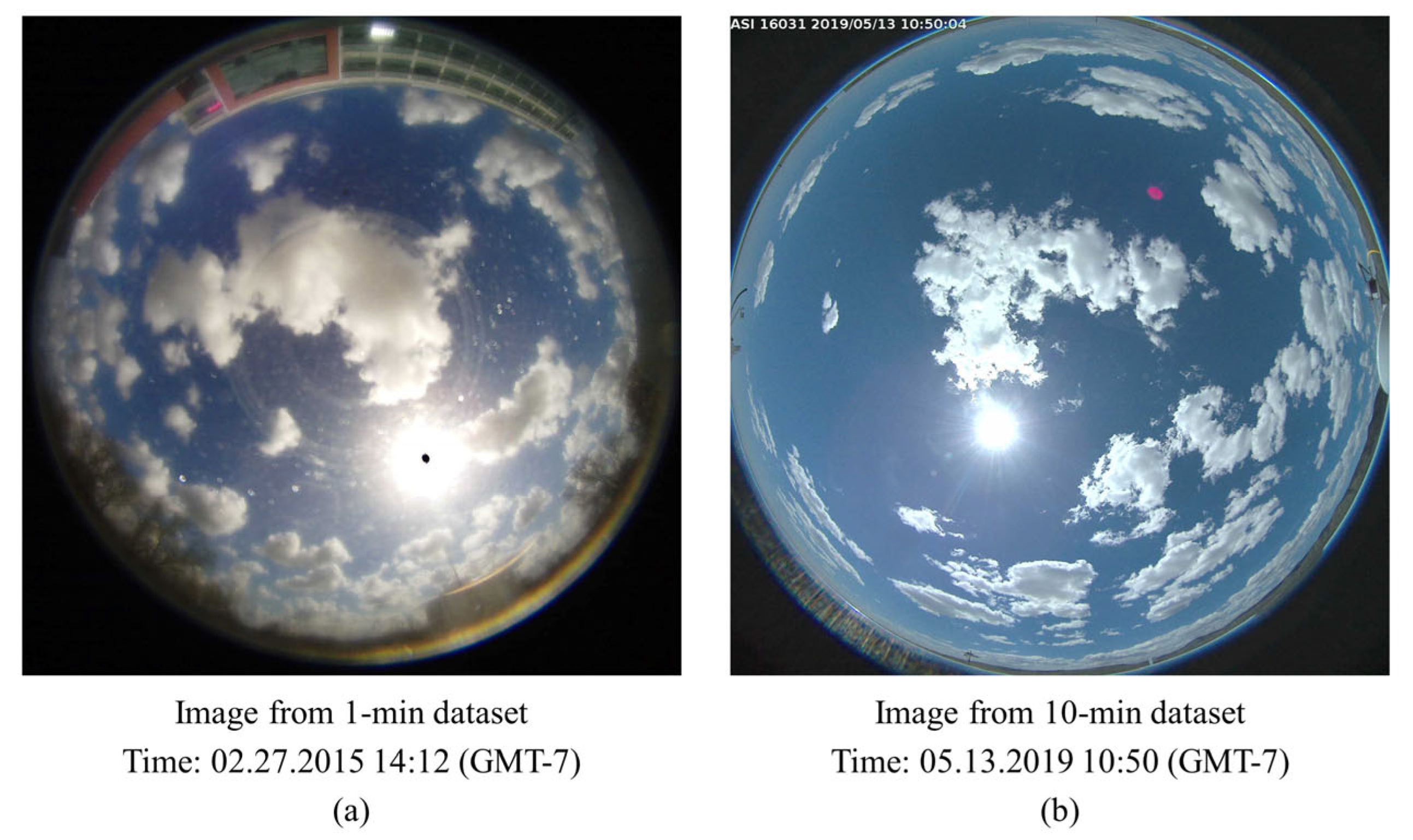
According to the temporal resolutions of the original images, two image sequence datasets were constructed. The 1-min dataset contained 300 image sequences from 2014 to 2016, and each sequence contained 10 consecutive images under cloudy conditions, as shown in Figure 1a. The 10-min dataset contained 300 image sequences from 2019 to 2021, and each sequence contained six consecutive images under cloudy conditions, as shown in Figure 1b.

Each image sequence was further converted into a 3D voxel cumulus cloud sequence [22]. During the modeling process, the ground-based sky images were first preprocessed to extract the cumulus cloud regions through lens distortion correction and solar glare removal. The 3D cumulus modeling parameters, including cloud-base height and cloud thickness, were then calculated based on the geographic location and imaging time of the ground-based sky imager. Finally, 3D voxel cumulus cloud models were constructed, and relative cloud-particle density was assigned to each voxel.

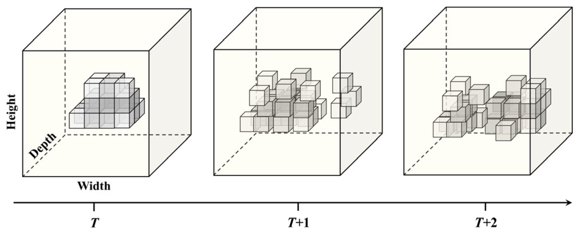
Based on this process, a 3D voxel cumulus cloud sequence dataset was constructed, as shown in Figure 2. The dataset contains both spatial and temporal information. The spatial information is represented by the position of each voxel in 3D space, namely the x, y, and z dimensions, whereas the temporal information is represented by consecutive observation time steps. The voxel value represents the estimated relative cloud-particle density.

The 3D voxel cumulus cloud sequences were organized as 6D tensors with the shape of (S, B, C, D, H, W) where S denotes the sequence length, B denotes the batch size, C denotes the number of channels, and D, H, and W denote the depth, height, and width of the voxel grid, respectively. Considering the large data volume of 3D voxel sequences and the computational cost of 3D recurrent networks, all voxel cloud models were uniformly resampled into 64 × 64 × 64 voxel blocks before model training. Here, 64 × 64 × 64 denotes the standardized input size for deep learning.

2.2. Wind Vector Dataset

To investigate the influence of horizontal wind on cumulus cloud motion and deformation, a wind-vector dataset was constructed from wind speed and wind direction data. The original wind data were obtained from the publicly available Derived Motion Wind (DMW) product of the GOES-16 satellite of the National Oceanic and Atmospheric Administration (NOAA). The DMW product is generated by tracking cloud features and water vapor gradients from sequences of visible or infrared spectral bands. It provides wind speed and wind direction information in netCDF-4 format with a temporal resolution of 30 min.

Because the DMW product has a temporal resolution of 30 min, whereas the 10-min cumulus cloud dataset has a finer temporal interval, each DMW wind record was matched to the corresponding 10-min cloud sequences within the same 30-min window. This study focuses on cumulus cloud evolution related to solar irradiance nowcasting, rather than precipitation systems, severe convective clouds, or storm-scale cloud processes. Accordingly, wind speed and wind direction were assumed to remain unchanged within each 30-min interval and were used as large-scale horizontal motion constraints for cumulus cloud advection.

The DMW product was matched with the spatial and temporal range of the 10-min cumulus cloud dataset. The 10-min dataset covers the sky-image observation range of 39.6417–39.8384° N and 105.0522–105.3079° W during 2019–2021. Because DMW retrieval points may be sparse within this area, the candidate spatial range was extended to 38–40° N and 104–106° W. Wind speed, wind direction, and geographic location information were then extracted from DMW records at the nearest observation times.

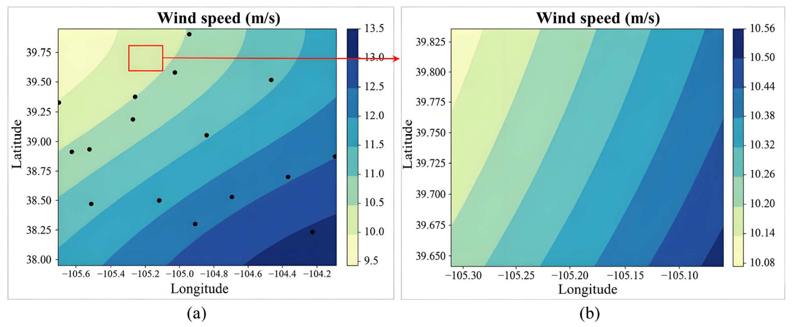
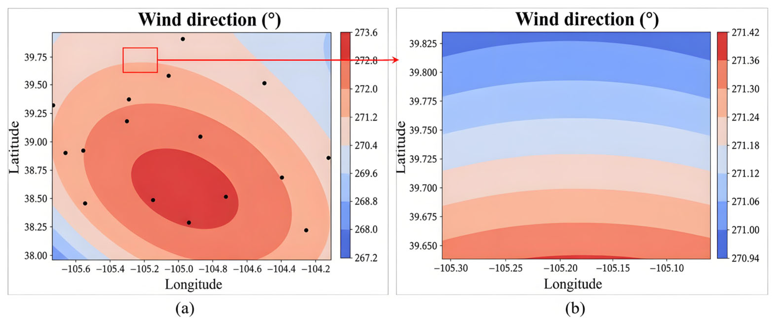
To obtain regional wind information, Kriging interpolation [25] was applied to the DMW point data within the candidate range. Figure 3 and Figure 4 show examples of the interpolated wind speed and wind direction at 14:10 (GMT-7) on May 5, 2019. The red boxes indicate the actual spatial extent of the 10-min cumulus cloud dataset. To construct a unified wind input for each 3D cumulus cloud sequence, the median wind speed and wind direction within the actual observation range were used to represent the wind conditions at the corresponding time step. For example, at 14:10 (GMT-7) on May 5, 2019, the representative wind speed and wind direction were 10.31 m/s and 271.18°, respectively.

Finally, wind speed and wind direction were matched with the time steps of the 3D voxel cumulus cloud sequences to form the wind input tensor (S, B, windSp, windDir) for WindGRU. Here, S denotes the sequence length, B denotes the number of sequences or batch size, and windSp and windDir denote wind speed and wind direction in the horizontal direction, respectively. Wind speed and wind direction were used because they are directly provided by the DMW product and were adopted as the native wind input variables in this study.

The input tensors used in this study are summarized in

Table 1. Summary of input tensors used in this study.

Input Data	Size/Tensor Form	Description/Unit
3D cumulus cloud sequence	(S, B, C, D, H, W), D = H = W = 64	Voxel value representing the reconstructed cloud distribution
Wind input	(S, B, windSp, windDir)	windSp: wind speed, m/s; windDir: wind direction, °

Note: S, B, C, D, H and W denote sequence length, batch size, channel number, depth, height, and width, respectively.

.

3. Methodology

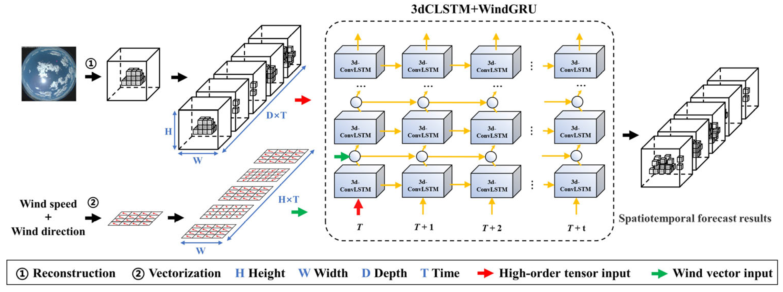
This study proposes an ultra-short-term spatiotemporal forecasting method for 3D cumulus clouds based on 3dCLSTM + WindGRU. The overall architecture is shown in Figure 5. The proposed model consists of two main components: a 3dCLSTM backbone for learning volumetric spatiotemporal features from 3D cumulus cloud sequences, and a WindGRU unit for incorporating wind speed and wind direction information into transient motion modeling.

The 3dCLSTM backbone is constructed using 3D convolutional LSTM units as the basic recurrent modules. It takes high-dimensional tensors composed of the height, width, depth, and temporal sequence of 3D cumulus clouds as input, and learns the motion and morphological changes of cumulus clouds through recurrent state transmission. On this basis, wind speed and wind direction are vectorized as supplementary meteorological inputs and introduced into the model through WindGRU. The WindGRU unit receives the hidden motion feature output from the upper 3D-ConvLSTM layer and the corresponding wind vector, and then generates a wind-corrected transient motion state for the next layer. In this way, the proposed model combines the long-term spatiotemporal evolution learned from historical 3D cloud sequences with the transient motion correction driven by wind information.

3.1. 3dCLSTM-Based Spatiotemporal Forecasting Network for 3D Cumulus Clouds

Spatiotemporal forecasting aims to predict future states by jointly modeling spatial and temporal information [26]. Ground-based sky images are usually acquired at intervals of 1–10 min to forecast cumulus cloud deformation over the following time steps. Similarly, ultra-short-term forecasting of 3D cumulus clouds uses reconstructed 3D cumulus cloud sequences as input. Therefore, this task can be regarded as a high-dimensional spatiotemporal sequence forecasting problem.

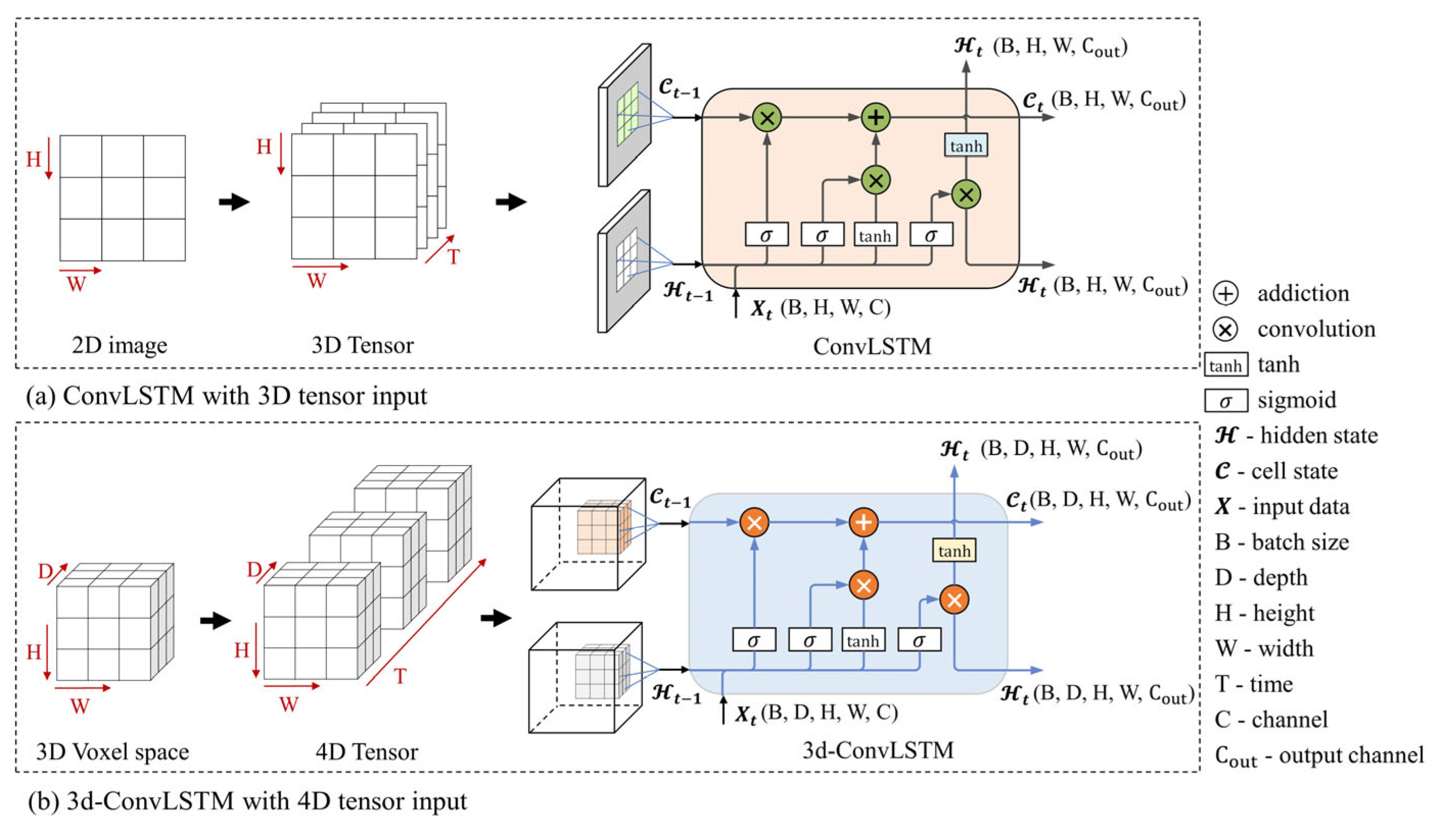
To forecast the motion and morphological changes of 3D cumulus clouds, this study constructs a multilayer recurrent network framework, termed 3dCLSTM, using 3D convolutional LSTM (3D-ConvLSTM) as the base unit. ConvLSTM [27] can effectively capture spatiotemporal correlations and has been widely used in image sequence prediction, including cloud image sequence forecasting [10,11,12]. However, conventional ConvLSTM is designed for 2D image sequences and generally accepts tensors composed of image height, image width, and channel information, as shown in Figure 6a. For 3D cumulus cloud sequences, the input contains an additional depth dimension. Therefore, ConvLSTM is extended to 3D-ConvLSTM to satisfy the input requirements of high-dimensional tensors composed of height, width, depth, and channel information, as shown in Figure 6b.

Using 3D-ConvLSTM as the basic recurrent unit, a multilayer recurrent network structure is constructed. Inspired by PredRNN [16], multiple 3D-ConvLSTM units are stacked to extract spatiotemporal features layer by layer, while memory states are transmitted horizontally along the temporal direction and vertically across network layers. This recurrent state transmission enables the model to learn the continuous evolution of 3D cumulus cloud morphology over time.

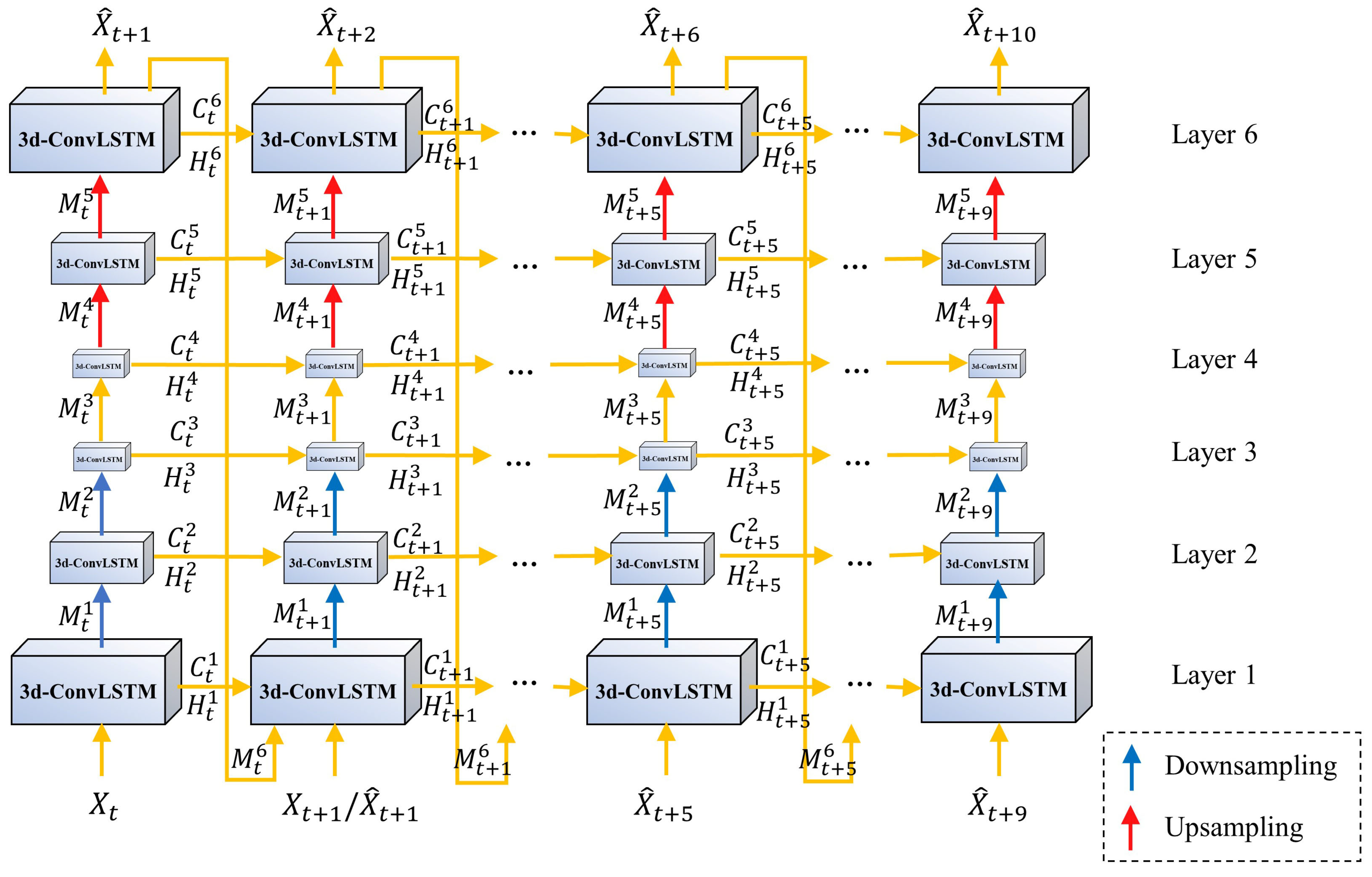
Considering the large data volume of 3D cumulus cloud sequences, direct recurrent learning on voxel data results in high computational cost and memory consumption. Therefore, a multiscale processing strategy is introduced into 3dCLSTM. As shown in Figure 7, max pooling is used for downsampling in lower layers to reduce spatial resolution and computational burden, while trilinear interpolation is used for upsampling in higher layers to restore the feature size. This structure allows the network to learn high-level volumetric features while maintaining the ability to output predicted cloud volumes at the original voxel resolution.

Figure 7 illustrates the main architecture of 3dCLSTM using a 10-step 3D cumulus cloud sequence as an example, where five historical time steps are used to predict the following five time steps. The network consists of six stacked 3D-ConvLSTM layers, in which recurrent states are transmitted both along the temporal direction and across network layers. The horizontal arrows represent the propagation of the cell state and hidden state to the next moment, while the vertical arrows indicate the transfer of memory states between adjacent layers. The memory state of the top layer is further passed to the bottom layer to the time step, while the vertical arrows represent the transfer of memory states between adjacent layers. The memory state from the top layer is further passed to the bottom layer at the next time step, forming a recurrent spatiotemporal memory flow. During training, scheduled sampling [28] is adopted, where the input at each prediction step is randomly selected from either the ground truth or the previously predicted output to improve model robustness.

In summary, 3dCLSTM extends ConvLSTM from 2D image sequence prediction to 3D voxel sequence prediction. By stacking 3D-ConvLSTM units and introducing multiscale downsampling and upsampling operations, the model can learn volumetric cloud motion and deformation while reducing the computational burden of high-dimensional sequence learning.

3.2. WindGRU-Based Wind-Aware Transient Motion Unit

The motion and shape of cumulus clouds change over time and are also influenced by external meteorological factors. In ultra-short-term forecasting, wind speed and wind direction are important factors affecting cloud displacement and deformation. Although 3dCLSTM can learn motion trends from historical 3D cloud sequences, it does not explicitly incorporate wind-driven motion information. Therefore, this study introduces a WindGRU unit to strengthen the transient motion modeling capability of the network.

The WindGRU unit is inspired by motion modeling in recurrent video prediction [19]. In this study, WindGRU is designed to fuse two types of information: the cloud motion feature learned from the hidden state of the 3D-ConvLSTM layer and the wind vector derived from wind speed and wind direction. The hidden state provides motion trend information learned from historical 3D cumulus cloud sequences, while the wind vector provides external directional and magnitude information related to cloud displacement. By fusing these two types of information, WindGRU generates a wind-corrected transient motion state and transmits it to the next recurrent layer.

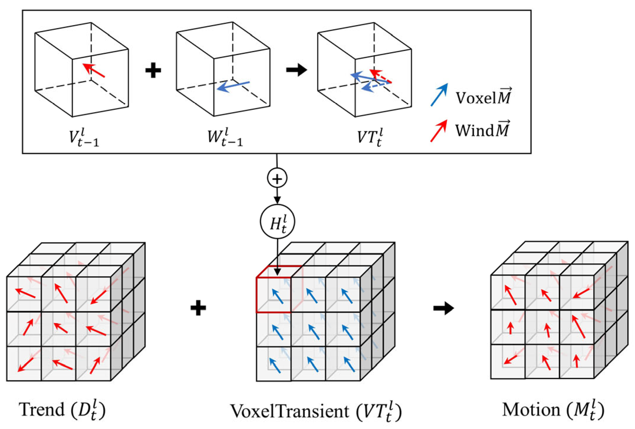
The wind-vector-driven transient motion feature is illustrated in Figure 8. In this process, the voxel motion vector derived from the displacement between two adjacent 3D cloud states is combined with the wind vector transformed from wind speed and wind direction. The resulting VoxelTransient feature is then added to the long-term motion trend to update the motion state transmitted in the recurrent network.

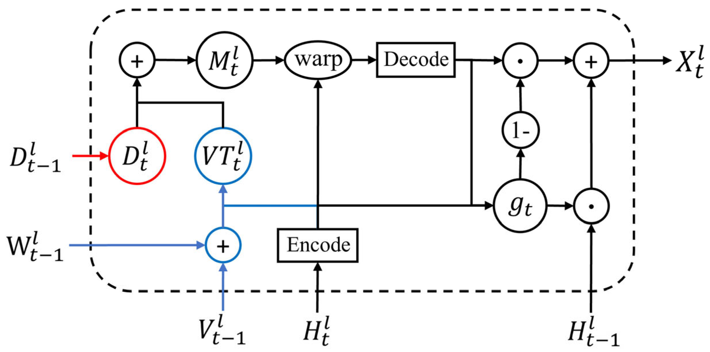
The structure of the WindGRU unit is shown in Figure 9. The unit adopts an encoder–decoder structure to reduce memory consumption and maintain feature consistency. The encoder compresses the hidden motion feature output from the preceding 3D-ConvLSTM layer. The wind vector is then broadcast and fused with the encoded motion feature to generate a wind-aware motion representation. Finally, the decoder restores the representation to the original hidden-state size and outputs the corrected transient motion state.

As shown in Figure 9, WindGRU updates the motion representation by integrating voxel transient motion, wind information, and motion trend. The voxel transient motion feature is corrected by the wind vector to obtain $V{T}_t^l$, and $V{T}_t^l$ is then combined with the motion trend $D_t^l$ to update the motion state $M_t^l$. The updated $M_t^l$ guides the warp operation on the encoded hidden feature. The warped feature is decoded and fused with the previous hidden feature through the output gate $g_t$ to generate $X_t^l$.

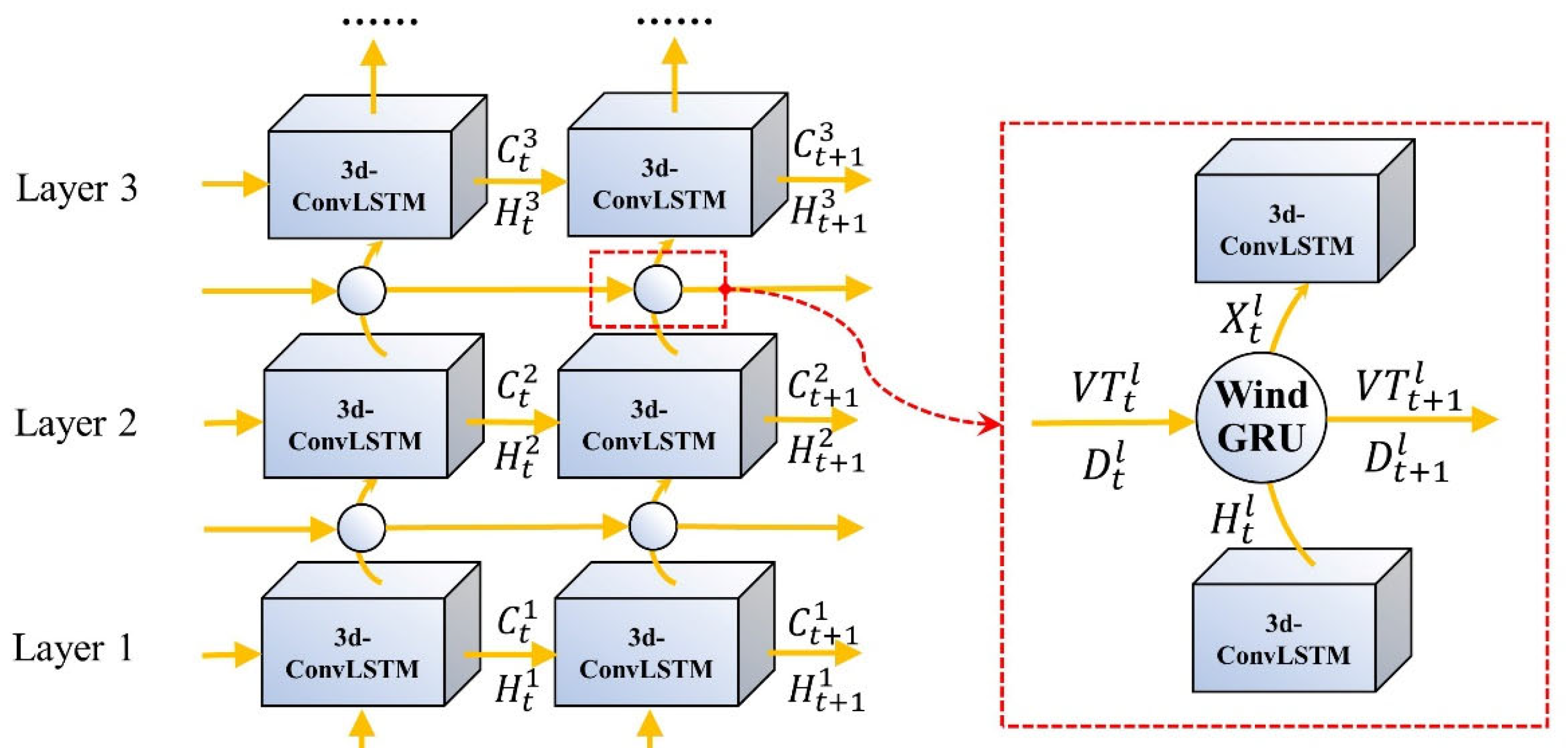
After being embedded between the layers of 3dCLSTM, WindGRU updates the transient motion state along the temporal direction and transfers the corrected motion state across network layers, as shown in Figure 10. In the vertical direction, the hidden state output from the preceding 3D-ConvLSTM layer is used as the input to WindGRU, and the wind-corrected motion state is passed to the next layer. In the horizontal direction, the transient motion state is continuously updated over time. Through this recurrent update mechanism, wind information is incorporated into the temporal evolution of 3D cumulus cloud motion.

In summary, WindGRU incorporates wind speed and wind direction as external motion constraints into the 3dCLSTM framework. The 3dCLSTM backbone learns the long-term volumetric evolution of cumulus clouds from historical sequences, while WindGRU corrects the transient motion state between adjacent time steps using wind information. The resulting 3dCLSTM + WindGRU model can therefore improve the representation of wind-driven cumulus cloud displacement and deformation in ultra-short-term 3D cloud forecasting.

4. Experiments

The proposed ultra-short-term spatiotemporal forecasting method for 3D cumulus clouds was evaluated from three aspects: the feasibility of 3dCLSTM for 3D cumulus cloud sequence forecasting, the effectiveness of incorporating WindGRU into 3dCLSTM, and the computational performance of the multiscale recurrent structure.

Six spatiotemporal forecasting models were compared, including ConvLSTM [27], PredRNN [16], PredRNN++ [17], single-scale 3dCLSTM, 3dCLSTM, and 3dCLSTM + WindGRU. ConvLSTM, PredRNN, and PredRNN++ were used as representative baseline models for spatiotemporal sequence prediction. Because these models were originally designed for 2D time-series data, their basic recurrent units were extended to 3D-ConvLSTM units according to the method described in Section 3, enabling them to accept high-dimensional 3D cumulus cloud sequence inputs. The single-scale 3dCLSTM was used to evaluate the effect of the multiscale structure, while 3dCLSTM without WindGRU was used as the baseline for evaluating the contribution of wind speed and wind direction information.

4.1. Implementation Details and Evaluation Metrics

This section summarizes the implementation environment, model hyperparameters, input-output settings, and evaluation metrics used for model training and testing.

To ensure a fair comparison, all forecasting models were trained using the same experimental settings. The batch size was set to 4, the convolutional kernel size was set to 3, and the hidden size was set to 130. Scheduled sampling [28] was adopted during training, and each model was trained for 300 epochs. These hyperparameters were determined by considering preliminary trial experiments, validation stability, and the memory constraints of 3D recurrent learning. The batch size of 4 was mainly constrained by the high GPU memory consumption of 3D voxel sequence forecasting. The hidden size of 130 was adopted as a balance between model capacity and memory usage, while the convolutional kernel size of 3 was used to capture local spatial features with controlled model complexity. All experiments were implemented in Python 3.9 using PyTorch with CUDA 10.2 support and conducted on four NVIDIA Tesla V100 GPUs with 16 GB memory. The implementation used CUDA-enabled multi-GPU distributed training, and the model modules were implemented based on PyTorch neural network components.

Two 3D cumulus cloud datasets with different temporal resolutions were used in the experiments, namely the 1-min and 10-min datasets described in Section 2. Each dataset was divided into training, validation, and test sets at a ratio of 7:1:2. Considering the computational cost and memory consumption of 3D recurrent learning, all voxel cloud data were resampled to a resolution of 64 × 64 × 64. The 1-min dataset contained 300 sequences, each consisting of 10 time steps. The first five time steps were used as historical inputs, and the following five time steps were used as prediction targets. The 10-min dataset contained 300 sequences, each consisting of six time steps. The first three time steps were used as historical inputs, and the following three time steps were used as prediction targets.

Because matched wind vector data were unavailable for the 1-min dataset, 3dCLSTM + WindGRU was evaluated only on the 10-min dataset. Accordingly, the 1-min dataset was used to assess the basic 3D spatiotemporal forecasting ability of 3dCLSTM, while the 10-min dataset was used to evaluate the effect of incorporating wind information into the forecasting model.

Based on these experimental settings, the evaluated models were organized into two groups. ConvLSTM, PredRNN, and PredRNN++ were used as baseline models to provide performance references for spatiotemporal sequence forecasting. Single-scale 3dCLSTM, 3dCLSTM, and 3dCLSTM + WindGRU were used for ablation-related comparison to examine the effects of the multiscale structure and wind information.

The models were optimized using a combination of L1 and L2 losses, corresponding to mean absolute error (MAE) and mean squared error (MSE), respectively. MSE and MAE were used to measure prediction errors, with smaller values indicating better performance. The structural similarity index measure (SSIM) and peak signal-to-noise ratio (PSNR) were further used to evaluate the structural similarity and reconstruction quality of the predicted 3D cloud volumes, with higher values indicating better performance.

4.2. Results

The quantitative evaluation results of the different models on the 1-min and 10-min cumulus cloud datasets are shown in

Table 2. Quantitative evaluation of different methods on the 1-min and 10-min cumulus cloud datasets.

		Sequence	1-min Dataset	10-min Dataset
	Method
SSIM	ConvLSTM		0.7744	0.3229
	PredRNN		0.7809	0.3195
	PredRNN++		0.7730	0.3180
	Single-scale 3dCLSTM		0.7791	0.3253
	3dCLSTM		0.7913	0.3351
	3dCLSTM + WindGRU		-	0.3512
PSNR	ConvLSTM		24.8582	17.7151
	PredRNN		25.1699	18.0071
	PredRNN++		24.9396	17.9490
	Single-scale 3dCLSTM		25.0730	18.0192
	3dCLSTM		25.4959	18.1162
	3dCLSTM + WindGRU		-	18.3625
MSE	ConvLSTM		16.9893	73.3438
	PredRNN		15.7707	68.9098
	PredRNN++		16.1258	69.5071
	Single-scale 3dCLSTM		16.1789	68.9715
	3dCLSTM		14.8906	67.4469
	3dCLSTM + WindGRU		-	67.0235
MAE	ConvLSTM		155.3853	375.4000
	PredRNN		147.3611	365.8554
	PredRNN++		151.5492	364.1609
	Single-scale 3dCLSTM		146.8905	360.7414
	3dCLSTM		140.3575	358.3522
	3dCLSTM + WindGRU		-	357.5698

Note: Bold values indicate the best performance for each metric.

. On the 1-min dataset, 3dCLSTM achieved the best performance among the models without wind information. Its SSIM reached 0.7913, which was 2.18%, 1.33%, and 2.37% higher than those of ConvLSTM, PredRNN, and PredRNN++, respectively. The PSNR of 3dCLSTM reached 25.4959, while the MSE and MAE decreased to 14.8906 and 140.3575, respectively. These results indicate that the 3dCLSTM framework can effectively support ultra-short-term forecasting of 3D cumulus cloud sequences.

On the 10-min dataset, incorporating wind speed and wind direction further improved the forecasting performance. The SSIM of 3dCLSTM + WindGRU reached 0.3512, which was 4.8% higher than that of 3dCLSTM without WindGRU. Compared with ConvLSTM, PredRNN, and PredRNN++, the SSIM increased by 8.77%, 9.93%, and 10.43%, respectively. The PSNR of 3dCLSTM + WindGRU reached 18.3625, and the MSE and MAE decreased to 67.0235 and 357.5698, respectively, which were the best results on the 10-min dataset. These results indicate that wind information can improve the forecasting accuracy of 3D cumulus cloud sequences at longer temporal intervals.

To further analyze forecasting performance at different prediction steps, the SSIM values at each step were compared, as shown in

Table 3. SSIM values at different prediction steps for different models.

		Sequence	t + 1	t + 2	t + 3	t + 4	t + 5
	Method
1-min dataset	ConvLSTM		0.8682	0.7559	0.6739	0.6205	0.5848
	PredRNN		0.8803	0.7640	0.6827	0.6335	0.5993
	PredRNN++		0.8622	0.7585	0.6876	0.6426	0.6087
	Single-scale 3dCLSTM		0.8786	0.7588	0.6781	0.6261	0.5908
	3dCLSTM		0.8907	0.7809	0.7009	0.6472	0.6076
	3dCLSTM + WindGRU		-	-	-	-	-
10-min dataset	ConvLSTM		0.3275	0.2995	0.3056	-	-
	PredRNN		0.3302	0.3027	0.3071	-	-
	PredRNN++		0.3222	0.3013	0.3057	-	-
	Single-scale 3dCLSTM		0.3386	0.3093	0.3052	-	-
	3dCLSTM		0.3310	0.2975	0.3022	-	-
	3dCLSTM + WindGRU		0.3512	0.3252	0.3126	-	-

Note: Bold values indicate the best SSIM at each prediction step.

. For the 1-min dataset, five historical time steps were used to predict five future time steps. For the 10-min dataset, three historical time steps were used to predict three future time steps. In general, the best forecasting performance was obtained at the first prediction step, and the accuracy decreased as the forecasting horizon increased.

For the 1-min dataset, 3dCLSTM achieved the highest SSIM values at most prediction steps. For the 10-min dataset, 3dCLSTM + WindGRU achieved the highest SSIM values at all three prediction steps. Compared with 3dCLSTM, incorporating WindGRU increased the SSIM from 0.3310 to 0.3512 at t + 1, from 0.2975 to 0.3252 at t + 2, and from 0.3022 to 0.3126 at t + 3. These results further indicate that wind information can improve step-wise forecasting performance.

To evaluate the influence of wind conditions on forecasting performance, 3dCLSTM and 3dCLSTM + WindGRU were compared using representative test samples selected from the 10-min dataset. As shown in

Table 4. Quantitative evaluation of wind effects on forecasting performance.

Wind Speed (m/s)	Wind Direction (°)	SSIM		PSNR
		3dCLSTM	3dCLSTM + WindGRU	3dCLSTM	3dCLSTM + WindGRU
3.698	270.606	0.3245	0.3332 (↑2.68%)	17.2151	17.1912 (↓0.14%)
4.913	299.809	0.3265	0.3326 (↑1.87%)	16.9245	16.8621 (↓0.37%)
5.268	319.088	0.3301	0.3236 (↓1.97%)	17.2355	17.2351 (-)
6.776	42.459	0.3198	0.3409 (↑6.60%)	16.8878	17.0355 (↑0.87%)
7.528	158.524	0.3292	0.3451 (↑4.83%)	16.9287	17.2115 (↑1.67%)
8.659	325.253	0.3224	0.3658 (↑13.46%)	17.0256	17.9812 (↑5.61%)
9.765	189.252	0.3186	0.3571 (↑12.08%)	16.8991	18.1454 (↑7.37%)
10.102	193.242	0.3199	0.3548 (↑10.91%)	16.6575	18.5183 (↑11.17%)

, each row corresponds to one representative test sample, and the listed wind speed and wind direction are the representative wind values matched to that sample. Eight test samples were selected, with wind speeds ranging from approximately 3 to 10 m/s. These samples were used to compare model performance under low-, medium-, and high-wind-speed conditions and to illustrate the sensitivity of the proposed model to wind speed. The values in parentheses indicate the relative changes in the results of 3dCLSTM + WindGRU compared with those of 3dCLSTM.

The results show that when the wind speed was relatively low, approximately 3–5 m/s, the improvement achieved by WindGRU was limited, and slight performance fluctuations occurred in some cases. As the wind speed increased, the advantage of 3dCLSTM + WindGRU became more evident. When the wind speed exceeded 8 m/s, SSIM increased by approximately 10.91–13.46%, and PSNR increased by approximately 5.61–11.17%. These results suggest that wind information contributes more strongly to 3D cumulus cloud forecasting under higher wind-speed conditions.

Finally, the computational performance of the evaluated models was analyzed in terms of parameter size and GPU memory usage, as shown in

Table 5. Comparison of training cost for the 10-min dataset.

Models	Params	Memory
ConvLSTM	152.07 M	18.69 GB
PredRNN	261 M	20.45 GB
PredRNN++	265.18 M	21.50 GB
Single-scale 3dCLSTM	1595.42 M	62.28 GB
3dCLSTM	1595.42 M	48.30 GB
3dCLSTM + WindGRU	1652.42 M	50.28 GB

. Because 3D spatiotemporal forecasting requires high memory consumption, the multiscale structure was introduced into 3dCLSTM to improve the computational feasibility of volumetric sequence learning.

Compared with ConvLSTM, PredRNN, and PredRNN++, the 3dCLSTM-based models had larger parameter sizes because they used 3D convolutional recurrent structures to process volumetric cloud sequences. The single-scale 3dCLSTM had the highest memory usage, reaching 62.28 GB during training. After the multiscale structure was introduced, the memory usage of 3dCLSTM decreased to 48.30 GB, corresponding to a reduction of approximately 22.45%. Although 3dCLSTM + WindGRU required slightly more parameters and memory than 3dCLSTM because of the additional WindGRU unit, its memory usage remained lower than that of the single-scale 3dCLSTM while it achieved better forecasting performance on the 10-min dataset. These results indicate that the proposed multiscale wind-aware structure improves 3D forecasting performance while maintaining computational feasibility.

In summary, the experimental results demonstrate the feasibility of 3dCLSTM for ultra-short-term 3D cumulus cloud forecasting and confirm the effectiveness of WindGRU in incorporating wind speed and wind direction information. The results also show that the multiscale structure can reduce memory consumption and improve the practicality of high-dimensional 3D sequence forecasting.

5. Discussion

The lower accuracy on the 10-min dataset indicates the difficulty of long-interval volumetric cloud forecasting. Compared with the 1-min dataset, the 10-min sequences contain larger displacement and morphological changes between adjacent cloud states, increasing the uncertainty of recurrent prediction. This result suggests that high-temporal-resolution observations are important for ultra-short-term 3D cumulus cloud forecasting. Therefore, the relatively low SSIM values on the 10-min dataset mainly reflect the increased difficulty of long-interval 3D voxel cloud forecasting, and the results on this dataset should be interpreted through comparisons among models under the same temporal-resolution setting.

The improvement achieved by 3dCLSTM + WindGRU suggests that wind speed and wind direction provide useful external motion constraints for 3D cloud forecasting. While 3dCLSTM learns motion trends from historical voxel sequences, WindGRU helps correct the transient motion state between adjacent time steps by introducing wind-related directional and magnitude information. The wind-speed sensitivity analysis further indicates that the improvement becomes more evident under relatively high wind-speed conditions, which is consistent with the physical understanding that wind is an important driver of low-altitude cumulus cloud displacement and deformation. The model complexity results also show that the multiscale structure is necessary for reducing the memory burden of 3D recurrent learning. This finding is consistent with recent advances in AI-based atmospheric nowcasting, where high-dimensional sequence learning, multi-source inputs, external physical variables, and computational efficiency are increasingly emphasized [20].

From the perspective of practical forecasting applications, the proposed method provides wind-aware 3D cloud evolution information to support subsequent solar irradiance nowcasting and PV power fluctuation analysis. Unlike 2D sky image prediction, the 3D voxel representation can describe volumetric cloud structure, cloud thickness, and density-related spatial variations, which are important for analyzing short-term variations in solar irradiance and PV power. More broadly, the proposed framework demonstrates the potential of combining high-dimensional spatiotemporal representation with external domain variables for complex atmospheric time series forecasting.

Although the proposed 3dCLSTM + WindGRU model demonstrates the feasibility of wind-aware 3D cumulus cloud forecasting, several aspects require further improvement. First, the 3D voxel clouds used in this study were reconstructed from ground-based sky images rather than directly measured by 3D atmospheric instruments, and reconstruction uncertainty may affect the forecasting results. Second, all voxel clouds were resampled to 64 × 64 × 64, which may lead to the loss of fine-scale cloud boundary and density information. In addition, the wind vector dataset was derived from DMW products with a temporal resolution of 30 min, and the current model mainly considered horizontal wind speed and wind direction. For the cumulus cloud forecasting task considered in this study, this setting provides useful large-scale motion constraints for cloud advection, but it may not fully capture high-frequency gusts, turbulence, or rapid local cloud deformation. Vertical wind speed may also affect cloud growth, dissipation, and morphological evolution. Future work will further explore higher-resolution 3D cloud representation, more complete meteorological constraints such as vertical wind speed, humidity, temperature, and NWP-based atmospheric variables, and validation with solar irradiance or PV power observations.

6. Conclusions

This study proposed a wind-aware ultra-short-term spatiotemporal forecasting model for 3D cumulus clouds, termed 3dCLSTM + WindGRU. The model uses a multiscale 3dCLSTM network to learn the four-dimensional spatiotemporal features of 3D voxel cumulus cloud sequences and introduces a WindGRU unit to incorporate wind speed and wind direction into transient motion modeling. By integrating volumetric sequence learning with wind-driven motion correction, the proposed model provides a forecasting framework for predicting the motion and deformation of 3D cumulus clouds.

Experiments were conducted on 1-min and 10-min 3D cumulus cloud datasets to evaluate the proposed method. On the 1-min dataset, 3dCLSTM achieved the best performance among the models without wind information, with an SSIM of 0.7913 and a PSNR of 25.4959. On the 10-min dataset, 3dCLSTM + WindGRU achieved the best performance after matched wind vector data were introduced, with an SSIM of 0.3512 and a PSNR of 18.3625. Compared with 3dCLSTM, incorporating WindGRU improved the SSIM by 4.8% on the 10-min dataset. The wind-speed sensitivity analysis further showed that the improvement was more evident under relatively high wind-speed conditions. In addition, the multiscale structure reduced memory usage by approximately 22.45% compared with the single-scale 3dCLSTM, indicating its effectiveness in reducing the computational burden of 3D recurrent learning.

The results indicate that wind-aware volumetric spatiotemporal modeling can improve ultra-short-term cumulus cloud forecasting and provide a useful technical basis for atmospheric sequence forecasting and solar irradiance nowcasting. Future work will focus on improving the spatial resolution of 3D cloud sequences, introducing more complete meteorological constraints, and validating the forecasting results with solar irradiance and PV power observations.

References

1. Ebad, M.; Grady, W.M. Cloud shadow model for analysis of solar photovoltaic power variability in high-penetration PV distribution networks. In Proceedings of the 2016 IEEE Power and Energy Society General Meeting (PESGM), Boston, MA, USA, 17–21 July 2016; pp. 1–5. [Google Scholar] [CrossRef] [Scilit]
2. Xia, P.; Zhang, L.; Min, M.; Li, J.; Wang, Y.; Yu, Y.; Jia, S. Accurate nowcasting of cloud cover at solar photovoltaic plants using geostationary satellite images. Nat. Commun. 2024, 15, 510. [Google Scholar] [CrossRef] [Scilit] [PubMed]
3. Reikard, G.; Haupt, S.E.; Jensen, T. Forecasting ground-level irradiance over short horizons: Time series, meteorological, and time-varying parameter models. Renew. Energy 2017, 112, 474–485. [Google Scholar] [CrossRef] [Scilit]
4. Zhang, C.; Du, Y.; Chen, X.; Lu, D.D.-C. Cloud motion tracking system using low-cost sky imager for PV power ramp-rate control. In Proceedings of the 2018 IEEE International Conference on Industrial Electronics for Sustainable Energy Systems (IESES), Hamilton, New Zealand, 31 January–2 February 2018; pp. 493–498. [Google Scholar] [CrossRef] [Scilit]
5. Li, M.; Chu, Y.; Pedro, H.T.C.; Coimbra, C.F.M. Quantitative evaluation of the impact of cloud transmittance and cloud velocity on the accuracy of short-term DNI forecasts. Renew. Energy 2016, 86, 1362–1371. [Google Scholar] [CrossRef] [Scilit]
6. Chow, C.W.; Belongie, S.; Kleissl, J. Cloud motion and stability estimation for intra-hour solar forecasting. Sol. Energy 2015, 115, 645–655. [Google Scholar] [CrossRef] [Scilit]
7. Marquez, R.; Coimbra, C.F.M. Intra-hour DNI forecasting based on cloud tracking image analysis. Sol. Energy 2013, 91, 327–336. [Google Scholar] [CrossRef] [Scilit]
8. Zhang, R.; Ma, H.; Saha, T.K.; Zhou, X. Photovoltaic nowcasting with bi-level spatio-temporal analysis incorporating sky images. IEEE Trans. Sustain. Energy 2021, 12, 1766–1776. [Google Scholar] [CrossRef] [Scilit]
9. Kong, W.; Jia, Y.; Dong, Z.Y.; Meng, K.; Chai, S. Hybrid approaches based on deep whole-sky-image learning to photovoltaic generation forecasting. Appl. Energy 2020, 280, 115875. [Google Scholar] [CrossRef] [Scilit]
10. Lu, Z.; Wang, Z.; Li, X.; Zhang, J. A method of ground-based cloud motion prediction: CCLSTM + SR-Net. Remote Sens. 2021, 13, 3876. [Google Scholar] [CrossRef] [Scilit]
11. Zhen, Z.; Zhang, X.; Mei, S.; Chang, X.; Chai, H.; Yin, R.; Wang, F. Ultra-short-term irradiance forecasting model based on ground-based cloud image and deep learning algorithm. IET Renew. Power Gener. 2022, 16, 2604–2616. [Google Scholar] [CrossRef] [Scilit]
12. Kellerhals, S.A.; De Leeuw, F.; Rodriguez Rivero, C. Cloud nowcasting with structure-preserving convolutional gated recurrent units. Atmosphere 2022, 13, 1632. [Google Scholar] [CrossRef] [Scilit]
13. Zhang, Y.; Long, M.; Chen, K.; Xing, L.; Jin, R.; Jordan, M.I.; Wang, J. Skilful nowcasting of extreme precipitation with NowcastNet. Nature 2023, 619, 526–532. [Google Scholar] [CrossRef] [Scilit] [PubMed]
14. Dai, K.; Li, X.; Fang, J.; Ye, Y.; Yu, D.; Su, H.; Xian, D.; Qin, D.; Wang, J. Four-hour thunderstorm nowcasting using a deep diffusion model for satellite data. Proc. Natl. Acad. Sci. USA 2025, 122, e2517520122. [Google Scholar] [CrossRef] [Scilit] [PubMed]
15. Cheng, Y.-S.; Wang, L.-P.; Scovell, R.W.; Wright, D. Exploring the use of 3D radar measurements in predicting the evolution of single-core convective cells. Atmos. Res. 2024, 304, 107380. [Google Scholar] [CrossRef] [Scilit]
16. Wang, Y.; Long, M.; Wang, J.; Gao, Z.; Yu, P.S. PredRNN: Recurrent neural networks for predictive learning using spatiotemporal LSTMs. Adv. Neural Inf. Process. Syst. 2017, 30, 879–888. [Google Scholar]
17. Wang, Y.; Gao, Z.; Long, M.; Wang, J.; Yu, P.S. PredRNN++: Towards a resolution of the deep-in-time dilemma in spatiotemporal predictive learning. In Proceedings of the 35th International Conference on Machine Learning (ICML 2018), Stockholm, Sweden, 10–15 July 2018; PMLR: Cambridge, MA, USA, 2018; pp. 5123–5132. [Google Scholar] [CrossRef] [Scilit]
18. Wang, Y.; Zhang, J.; Zhu, H.; Long, M.; Wang, J.; Yu, P.S. Memory in memory: A predictive neural network for learning higher-order non-stationarity from spatiotemporal dynamics. In Proceedings of the IEEE/CVF Conference on Computer Vision and Pattern Recognition (CVPR), Long Beach, CA, USA, 15–20 June 2019; pp. 9154–9162. [Google Scholar] [CrossRef] [Scilit]
19. Wu, H.; Yao, Z.; Wang, J.; Long, M. MotionRNN: A flexible model for video prediction with spacetime-varying motions. In Proceedings of the IEEE/CVF Conference on Computer Vision and Pattern Recognition (CVPR), Nashville, TN, USA, 20–25 June 2021; pp. 15435–15444. [Google Scholar] [CrossRef] [Scilit]
20. An, S.; Oh, T.-J.; Sohn, E.; Kim, D. Deep learning for precipitation nowcasting: A survey from the perspective of time series forecasting. Expert Syst. Appl. 2025, 268, 126301. [Google Scholar] [CrossRef] [Scilit]
21. Kosmopoulos, P.; Dhake, H.; Melita, N.; Tagarakis, K.; Georgakis, A.; Stefas, A.; Vaggelis, O.; Korre, V.; Kashyap, Y. Multi-Layer Cloud Motion Vector Forecasting for Solar Energy Applications. Appl. Energy 2024, 353, 122144. [Google Scholar] [CrossRef] [Scilit]
22. Chen, Y.; Chen, J.; Huang, W. 3D cumulus cloud scene modeling and shadow analysis method based on ground-based sky images. Int. J. Appl. Earth Obs. Geoinf. 2022, 109, 102765. [Google Scholar] [CrossRef] [Scilit]
23. Pedro, H.T.C.; Larson, D.P.; Coimbra, C.F.M. A comprehensive dataset for the accelerated development and benchmarking of solar forecasting methods. J. Renew. Sustain. Energy 2019, 11, 036102. [Google Scholar] [CrossRef] [Scilit]
24. Andreas, A.; Stoffel, T. NREL Solar Radiation Research Laboratory (SRRL): Baseline Measurement System (BMS), Golden, Colorado (Data); NREL Report No. DA-5500-56488; National Renewable Energy Laboratory: Golden, CO, USA, 1981.
25. Oliver, M.A.; Webster, R. Kriging: A method of interpolation for geographical information systems. Int. J. Geogr. Inf. Syst. 1990, 4, 313–332. [Google Scholar] [CrossRef] [Scilit]
26. Xu, L.; Chen, N.; Chen, Z.; Zhang, C.; Yu, H. Spatiotemporal forecasting in earth system science: Methods, uncertainties, predictability and future directions. Earth-Sci. Rev. 2021, 222, 103828. [Google Scholar] [CrossRef] [Scilit]
27. Shi, X.; Chen, Z.; Wang, H.; Yeung, D.-Y.; Wong, W.-K.; Woo, W.-C. Convolutional LSTM network: A machine learning approach for precipitation nowcasting. Adv. Neural Inf. Process. Syst. 2015, 28, 802–810. [Google Scholar]
28. Bengio, S.; Vinyals, O.; Jaitly, N.; Shazeer, N. Scheduled sampling for sequence prediction with recurrent neural networks. Adv. Neural Inf. Process. Syst. 2015, 28, 1171–1179. [Google Scholar]
Figure 1. Sample of ground-based cloud images.
Applsci 16 06856 g001
Figure 2. Sketch of the 3D voxel cumulus time-series dataset.
Applsci 16 06856 g002
Figure 3. Wind speed interpolation results at 14:10 (GMT-7) on 5 May 2019. (a) Wind speed interpolation within the candidate spatial range, with black points representing DMW retrieval points and the red box indicating the spatial extent of the 10-min cumulus cloud dataset; (b) enlarged interpolation results within the dataset coverage area.
Applsci 16 06856 g003
Figure 4. Wind direction interpolation results at 14:10 (GMT-7) on 5 May 2019. (a) Wind direction interpolation within the candidate spatial range, with black points representing DMW retrieval points and the red box indicating the spatial extent of the 10-min cumulus cloud dataset; (b) enlarged interpolation results within the dataset coverage area.
Applsci 16 06856 g004
Figure 5. Overall architecture of the proposed 3dCLSTM + WindGRU model.
Applsci 16 06856 g005
Figure 6. Sketch of the ConvLSTM and 3D-ConvLSTM inputs.
Applsci 16 06856 g006
Figure 7. Architecture of the 3dCLSTM. X t denotes the input 3D voxel cloud at time step t , and X ^ t + i denotes the predicted 3D voxel cloud at a future time step. H t l , C t l , and M t l denote the hidden state, cell state, and memory state of the l -th layer, respectively. Blue and red arrows indicate downsampling and upsampling, respectively.
Applsci 16 06856 g007
Figure 8. Sketch of the wind-vector-driven transient motion feature. Each 3D tensor represents a volumetric voxel cloud at a single time step with spatial dimensions (D, H, W).
Applsci 16 06856 g008
Figure 9. Architecture of the WindGRU unit.
Applsci 16 06856 g009
Figure 10. Main architecture of 3dCLSTM + WindGRU.
Applsci 16 06856 g010