Variable Forgetting Factor RLS Adaptive Algorithms Based on Line Search Methods

Abstract

Recursive least-squares (RLS) adaptive algorithms are capable of outperforming least-mean-square (LMS) methods for the identification of long-length impulse responses due to their ability to mitigate the high correlation properties of input signals, such as speech. Despite the encouraging results obtained in terms of tracking speed and accuracy, with respect to LMS methods, most RLS algorithms manifest numerical stability issues. Moreover, when an unknown system changes, the identification process needs to adapt to the new impulse response as soon as possible. The algorithm can require a significant amount of time to generate new accurate results in acoustic echo cancellation (AEC) scenarios. Due to the slow propagation speed of sound, acoustic echo paths are usually modeled using thousands of numerical coefficients, and adaptation energy remains relatively limited. A compromise is usually made between tracking capabilities and steady-state accuracy when choosing the forgetting factor (the most important parameter of the RLS algorithm). This paper analyzes a variable forgetting factor (VFF) RLS type of adaptive filter combined with the conjugate gradient (CG) line search method, which is designed to avoid the classical matrix inversion approach. This VFF-RLS-CG adaptive method is not susceptible to numerical stability issues and is designed to adapt its statistical estimates by determining whether a tracking situation occurs or whether the unknown system is not significantly different. Correspondingly, when necessary, the forgetting factor is decreased for faster adaptation to changes in the working environment. When the filter is estimated to work at steady-state, the above-mentioned parameter’s value is increased in order to boost the accuracy of the adaptive filter. The theoretical model is validated using simulations in AEC scenarios with tracking occurrences and relevant steady-state intervals.

1. Introduction

Adaptive algorithms are employed in system identification configurations, such as acoustic echo cancellation (AEC) setups, in order to continuously track acoustic impulse responses and estimate their corresponding outputs [1,2]. An acoustic echo causes the speaker to hear a delayed replica of their own voice, which is caused by acoustic reflections created in the environment in which the other interlocutors are located.

Least-mean-square (LMS) adaptive methods are strongly preferred for hardware implementation in the industry, due to their reduced associated computational costs [3,4,5]. However, they offer poor performance when working with highly correlated input signals, such as in the case of speech. Consequently, a lot of research resources are invested in other types of adaptive algorithms, which are more capable of mitigating the statistical properties of the input signals.

Least-squares (LS) methods represent an attractive alternative to LMS, due to their abilities to “decorrelate” the input signals and achieve superior tracking speeds [1,6,7,8,9]. For example, the exponentially weighted recursive least-squares (RLS) algorithm based on Woodbury’s inversion lemma is often employed as a reference in research works, and it can outperform the popular normalized LMS (NLMS) algorithm in terms of tracking speed and steady-state accuracy. The memory of RLS adaptive algorithms is adjusted using their main parameter, the forgetting factor $\lambda$, which is usually chosen as a fixed value in the numerical interval $0<\lambda \le 1$ [1,4,10]. As the name would suggest, when $\lambda$ has a lower value, the memory of the RLS is reduced, and it has the benefit of adapting faster to potential changes in the unknown system. When $\lambda$ is closer to 1, the memory of the algorithm favors the accuracy at steady-state, when no relevant changes happen in the unknown impulse response. In the standard approach, a compromise is made between the two capabilities through the choice of a fixed value of $\lambda$.

Many RLS variants have several flaws, which make them prohibitive in practice. They manifest occasional numerical stability issues and have high computational requirements for hardware implementations (the corresponding arithmetic complexity is proportional to the square of the adaptive filter’s length). Consequently, an important part of the mentioned research effort is invested in alternative versions of the RLS, which can preserve the performances associated with the Woodbury RLS approach. Such is the case of exponentially weighted RLS methods combined with line search methods (LSMs) [6,8,11]. The RLS-LSM approach employs an alternative solution for the classical associated matrix inversion problem and is designed to favor iterative methods, which exploit the statistical properties of the input signals.

In this paper, the forgetting factor is analyzed as a variable value for the combination between the RLS and the conjugate gradient (CG) LSM [12,13]. The purpose is to present a method for adjusting $\lambda$ depending on the circumstances in which the adaptive system is working. If the tracking capabilities of RLS-CG need to be increased, the value of $\lambda$ is set to a lower value. Vice versa, at steady-state, the value of $\lambda$ is expected to increase and be closer to the value 1. The proposed solution requires no extra adjustment of other parameters or control mechanisms, as in the cases of other similar methods, which are difficult to apply in real-world scenarios [14,15,16,17,18,19,20,21].

Section 2 of this paper comprises a general presentation of RLS-LSM adaptive algorithms. In Section 3, the value of $\lambda$ is theoretically developed as a function of the discrete time index n [i.e., as $\lambda \left(n\right)$] in order to match the general criteria mentioned above. The proposed variable forgetting factor (VFF) approach [22] is applied to RLS-CG in Section 4, while the simulation results are presented in Section 5, in order to validate the VFF-RLS-CG adaptive algorithm. These simulation results are shown for AEC scenarios using different types of input signals and tracking scenarios. Conclusions are described in Section 6 with respect to the theoretical information, simulation results, and the implications for hardware applications.

2. RLS Algorithm with Line Search Methods

In the system identification process for AEC scenarios, the adaptive filter’s purpose is to estimate the unknown system defined by an impulse response vector $\mathbf{h}$ of length L. The reference (or microphone) signal is obtained as

$$\begin{array}{cc}\hfill d\left(n\right)& ={\mathbf{x}}^T\left(n\right)\mathbf{h}+v\left(n\right)=y\left(n\right)+v\left(n\right),\hfill \end{array}$$

(1)

where $\mathbf{x}\left(n\right)$ is a buffer vector containing the most recent L samples of the input signal, the superscript ^T denotes the transposition, and $v\left(n\right)$ is a zero-mean additive noise signal corrupting the output $y\left(n\right)$ of the system [1,4]. The noise is considered to be uncorrelated with the samples comprising $\mathbf{x}\left(n\right)$. The a priori error signal is defined as the following difference:

$$\begin{array}{cc}\hfill e\left(n\right)& =d\left(n\right)-{\mathbf{x}}^T\left(n\right)\widehat{\mathbf{h}}(n-1),\hfill \end{array}$$

(2)

where $d\left(n\right)$ is the reference (i.e., microphone) signal, and $\widehat{\mathbf{h}}\left(n\right)$ is the set of coefficients used to estimate the unknown impulse response $\mathbf{h}$. The LS approach for estimating $\mathbf{h}$ is associated with the minimization of the cost function:

$$\begin{array}{c}\hfill \mathcal{J}\left[\widehat{\mathbf{h}}\left(n\right)\right]={\displaystyle \sum _{i=1}^n}{\lambda }^{n-i}{\left[d\left(i\right)-{\mathbf{x}}^T\left(i\right)\widehat{\mathbf{h}}\left(n\right)\right]}^2,\end{array}$$

(3)

where $\lambda$ controls the memory of the algorithm and is called the forgetting factor. Minimizing the cost function leads to the following system of linear equations:

$$\begin{array}{c}\hfill \mathbf{R}\left(n\right)\widehat{\mathbf{h}}\left(n\right)=\mathbf{p}\left(n\right),\end{array}$$

(4)

where $\mathbf{R}\left(n\right)$ is the estimated $L\times L$ positive definite covariance matrix associated with the samples of the input signal $x\left(n\right)$, and $\mathbf{p}\left(n\right)$ is the $L\times 1$ cross-correlation vector between the samples of $\mathbf{x}\left(n\right)$ and $d\left(n\right)$ [1,2,6]. The known quantities in (4) are $\mathbf{R}\left(n\right)$ and $\mathbf{p}\left(n\right)$, which can be recursively updated using $\lambda$ as

$$\begin{array}{c}\hfill \mathbf{R}\left(n\right)=\lambda \mathbf{R}(n-1)+\mathbf{x}\left(n\right){\mathbf{x}}^T\left(n\right),\end{array}$$

(5)

$$\begin{array}{c}\hfill \mathbf{p}\left(n\right)=\lambda \mathbf{p}(n-1)+\mathbf{x}\left(n\right)d\left(n\right).\end{array}$$

(6)

In order to avoid applying direct solutions for solving the system in (4), the associated expression can be reinterpreted in order to solve an auxiliary system of equations [6,23]. New notations are introduced to track the variations in the covariance matrix $\mathbf{R}\left(n\right)$ and the cross-correlation vector $\mathbf{p}\left(n\right)$ from consecutive time indices:

$$\begin{array}{cc}\hfill \mathsf{\Delta }\mathbf{R}\left(n\right)& =\mathbf{R}\left(n\right)-\mathbf{R}(n-1)=(\lambda -1)\mathbf{R}\left(n\right)+\mathbf{x}\left(n\right){\mathbf{x}}^T\left(n\right),\hfill \end{array}$$

(7)

$$\begin{array}{cc}\hfill \mathsf{\Delta }\mathbf{p}\left(n\right)& =\mathbf{p}\left(n\right)-\mathbf{p}(n-1)=(\lambda -1)\mathbf{p}\left(n\right)+d\left(n\right)\mathbf{x}\left(n\right),\hfill \end{array}$$

(8)

where $\mathsf{\Delta }\mathbf{R}\left(n\right)$ is an $L\times L$ matrix, and $\mathsf{\Delta }\mathbf{p}\left(n\right)$ is an L-valued vector. Moreover, the variation in the filter’s coefficients between consecutive time indices is denoted using the $L\times 1$ vector:

$$\begin{array}{cc}\hfill \mathsf{\Delta }\mathbf{h}\left(n\right)& =\mathbf{h}\left(n\right)-\widehat{\mathbf{h}}(n-1).\hfill \end{array}$$

(9)

The new purpose is to replace the direct determination of the estimate $\widehat{\mathbf{h}}\left(n\right)$ with the computation of the estimate $\mathsf{\Delta }\widehat{\mathbf{h}}\left(n\right)$, which is called the solution vector. By considering that at time index n, the estimate $\widehat{\mathbf{h}}(n-1)$ is already known, the expression in (9) can be used in (4) to obtain

$$\begin{array}{c}\hfill \mathbf{R}\left(n\right)\mathsf{\Delta }\mathbf{h}\left(n\right)={\mathbf{p}}_0\left(n\right),\end{array}$$

(10)

where the $L\times 1$ residual component ${\mathbf{p}}_0\left(n\right)$ is defined as

$$\begin{array}{c}\hfill {\mathbf{p}}_0\left(n\right)=\mathbf{p}\left(n\right)-\mathbf{R}\left(n\right)\widehat{\mathbf{h}}(n-1).\end{array}$$

(11)

The system of equations in (10) is the new problem, which requires a solution in order to perform the adaptive filter update [7,8]. After $\mathsf{\Delta }\widehat{\mathbf{h}}\left(n\right)$ is determined, the column vector of filter coefficients can be updated, yielding $\widehat{\mathbf{h}}\left(n\right)$ as

$$\begin{array}{c}\hfill \widehat{\mathbf{h}}\left(n\right)=\widehat{\mathbf{h}}(n-1)+\mathsf{\Delta }\widehat{\mathbf{h}}\left(n\right).\end{array}$$

(12)

Solving (10) is equivalent to finding the global minimum of the quadratic function

$$\begin{array}{c}\hfill f\left[\mathsf{\Delta }\widehat{\mathbf{h}}\left(n\right)\right]={\displaystyle \frac{1}{2}}\mathsf{\Delta }{\widehat{\mathbf{h}}}^T\left(n\right)\mathbf{R}\left(n\right)\mathsf{\Delta }\widehat{\mathbf{h}}\left(n\right)-{\mathbf{p}}_0\left(n\right)\mathsf{\Delta }\widehat{\mathbf{h}}\left(n\right),\end{array}$$

(13)

by computing its gradient and setting it equal to zero [7]. The concept of the residual vector is also used as

$$\begin{array}{c}\hfill \mathbf{r}\left(n\right)=\mathbf{p}\left(n\right)-\mathbf{R}\left(n\right)\widehat{\mathbf{h}}\left(n\right),\end{array}$$

(14)

which is computed at the end of the adaptive filter’s iteration. The residual vector can be seen as an error measure regarding the accuracy of the adaptive filter at time index n and is part of the adaptation process at the next time index. Moreover, the residual component can be recursively expressed using (7) and (8), then (14), in (11), in order to obtain

$$\begin{array}{cc}\hfill {\mathbf{p}}_0\left(n\right)& =\mathbf{r}(n-1)+\mathsf{\Delta }\mathbf{p}\left(n\right)-\mathsf{\Delta }\mathbf{R}\left(n\right)\widehat{\mathbf{h}}(n-1)\hfill \\ \hfill & =\mathbf{r}(n-1)+(\lambda -1)\mathbf{p}(n-1)+d\left(n\right)\mathbf{x}\left(n\right)\hfill \\ \hfill & -(\lambda -1)\mathbf{R}(n-1)\widehat{\mathbf{h}}(n-1)-\mathbf{x}\left(n\right){\mathbf{x}}^T\left(n\right)\widehat{\mathbf{h}}(n-1)\hfill \\ \hfill & =\lambda \mathbf{r}(n-1)+\mathbf{x}\left(n\right)e\left(n\right),\hfill \end{array}$$

(15)

where it can be noticed that the update for ${\mathbf{p}}_0\left(n\right)$ can be performed with the most recent input samples, the error signal, and the residual vector from the previous time index [6].

The framework based on the described auxiliary system of equations is summarized in

Table 1. The RLS-LSM adaptive algorithm.

Step	Actions
	$\mathrm{Initialization}:$
	$\widehat{\mathbf{h}}\left(0\right)={\mathbf{0}}_{\mathit{L}\times 1}$
	$\mathbf{r}\left(0\right)={\mathbf{0}}_{\mathit{L}\times 1}$
	$\mathbf{R}\left(0\right)=\mathsf{\Phi }{\mathbf{I}}_{\mathit{L}},\mathsf{\Phi }>0$
	$\mathrm{For}n=1,2,\dots$
1	Update $\mathbf{x}\left(n\right)$
2	Update $\mathbf{R}\left(n\right)$ using (5)
3	$y\left(n\right)={\widehat{\mathbf{h}}}^T(n-1)\mathbf{x}\left(n\right)$
4	$e\left(n\right)=d\left(n\right)-y\left(n\right)$
5	${\mathbf{p}}_0\left(n\right)=\lambda \mathbf{r}(n-1)+e\left(n\right)\mathbf{x}\left(n\right)$
6	$\mathbf{R}\left(n\right)\mathsf{\Delta }\mathbf{h}\left(n\right)={\mathbf{p}}_0\left(n\right)\stackrel{\mathrm{LSM}}{\to }\mathsf{\Delta }\widehat{\mathbf{h}}\left(n\right),\mathbf{r}\left(n\right)$
7	$\widehat{\mathbf{h}}\left(n\right)=\widehat{\mathbf{h}}(n-1)+\mathsf{\Delta }\widehat{\mathbf{h}}\left(n\right)$

. The constant $\mathsf{\Phi }$ multiplied by the $L\times L$ identity matrix ${\mathbf{I}}_{\mathit{L}}$ is used for the initialization of $\mathbf{R}\left(0\right)$ and ensures the non-singular property of the matrix in the initial stages of the algorithm. The vectors $\widehat{\mathbf{h}}\left(0\right)$ and $\mathbf{r}\left(0\right)$ are initialized using zero-valued $L\times 1$ column vectors (${\mathbf{0}}_{\mathit{L}\times 1}$). The algorithm is suitable for using LSMs, which perform two roles: they compute the estimate $\mathsf{\Delta }\widehat{\mathbf{h}}\left(n\right)$ and provide an updated version of the residual vector $\mathbf{r}\left(n\right)$ (step 6). The RLS-LSM combination can exploit the properties of the input signals and does not manifest the numerical stability issues specific to the RLS based on Woodbury’s identity.

3. Variable Forgetting Factor for RLS-LSM Algorithms

In most RLS versions, the forgetting factor is chosen as a constant with the following form:

$$\begin{array}{cc}\hfill \lambda & =1-{\displaystyle \frac{1}{KL}},\hfill \end{array}$$

(16)

where the constant K is usually chosen as a non-zero natural number [22]. Considering that an adaptive filter for AEC scenarios can perform the update of thousands of coefficients, the possibility of dynamically improving the adaptation energy in tracking intervals, with respect to increasing the accuracy level in steady-state intervals, can allow for a customized behavior of the RLS in accordance with the environmental conditions. The purpose of the VFF approach is to define a mechanism for adjusting $\lambda \left(n\right)$ in order to obtain a good balance between tracking capabilities and accuracy at steady-state, depending on the most important requirement at the moment of the computation [22]. Different VFF-based techniques can be found in the literature, in the framework of various applications, e.g., see [21,24,25,26,27,28,29] and the references therein. Nevertheless, most of the existing VFF-RLS algorithms require extra tuning parameters related to the evaluation of their forgetting factors and/or additional decision mechanisms (e.g., threshold-based), which are not easy to handle in practice, especially in real-time applications.

The development of the expression for $\lambda \left(n\right)$ takes into consideration the basic RLS algorithm, which determines the error signal in (2) and updates the filter coefficients (with an arithmetic complexity proportional to the cube of L) as

$$\begin{array}{cc}\hfill \widehat{\mathbf{h}}\left(n\right)& =\widehat{\mathbf{h}}(n-1)+{\mathbf{R}}^{-1}\left(n\right)\mathbf{x}\left(n\right)e\left(n\right).\hfill \end{array}$$

(17)

Considering that the RLS-LSM family of adaptive methods is designed to achieve the performances of the basic RLS, the following considerations can be applied to the former method, just as in the case of the latter.

The a posteriori error can be expressed after each update of the filter coefficients as

$$\begin{array}{cc}\hfill ϵ\left(n\right)& =d\left(n\right)-{\mathbf{x}}^T\left(n\right)\widehat{\mathbf{h}}\left(n\right),\hfill \end{array}$$

(18)

which can also be written using (2) and (17)

$$\begin{array}{cc}\hfill ϵ\left(n\right)& =\left[1-{\mathbf{x}}^T\left(n\right){\mathbf{R}}^{-1}\left(n\right)\mathbf{x}\left(n\right)\right]e\left(n\right),\hfill \end{array}$$

(19)

then rewritten considering the form of the reference signal in (1) as

$$\begin{array}{cc}\hfill ϵ\left(n\right)& ={\mathbf{x}}^T\left(n\right)\left[\mathbf{h}-\widehat{\mathbf{h}}\left(n\right)\right]+v\left(n\right).\hfill \end{array}$$

(20)

In an ideal situation, the a posteriori error is equal to the noise influencing the microphone signal, i.e., $ϵ\left(n\right)=v\left(n\right)$. The condition was replaced in [22] by

$$\begin{array}{c}\hfill E\left[{ϵ}^2\left(n\right)\right]={\sigma }_v^2,\end{array}$$

(21)

where $E[·]$ expresses the mathematical expectation, and ${\sigma }_v^2$ is the noise power, which is considered to be constant.

In order to develop (21), several approximations will be employed considering the statistical properties of the input signal. Firstly, the covariance matrix is considered to be close to a diagonal matrix so that we can write

$$\begin{array}{c}\hfill E\left[\mathbf{x}\left(n\right){\mathbf{x}}^T\left(n\right)\right]\approx {\sigma }_x^2{\mathbf{I}}_{\mathit{L}},\end{array}$$

(22)

where ${\sigma }_x^2$ is the variance in the input signal. This represents a key approximation for the upcoming development. Indeed, this assumption holds especially for white Gaussian signals or mild correlated inputs, when the covariance matrix is close to a diagonal one. The reason behind using this approximation is basically twofold: (A) It allows for an important simplification of the development related to the VFF design, which results in a practical and easy way to handle the formula for the time-dependent forgetting factor. (B) Even for highly correlated input signals (like speech), when this assumption is biased, the resulting RLS-type algorithm still uses the full estimate of the covariance matrix based on (5) so that information about the true character of the input signal is still available. This aspect will also be supported in Section 5, in terms of the simulation results, showing that the proposed VFF-type algorithm obtains good performance for various inputs, including highly correlated ones (e.g., autoregressive processes with a pole very close to 1 and speech sequences).

Secondly, after the algorithm has run for a reasonable amount of time (i.e., for n large enough), the covariance matrix can be expressed as

$$\begin{array}{c}\hfill \mathbf{R}\left(n\right)\approx {(1-\lambda )}^{-1}{\sigma }_x^2{\mathbf{I}}_{\mathit{L}}.\end{array}$$

(23)

By also taking into consideration that $L\gg 1$, we can write

$$\begin{array}{c}\hfill {\mathbf{x}}^T\left(n\right)\mathbf{x}\left(n\right)\approx L{\sigma }_x^2.\end{array}$$

(24)

The approximations can be used to rewrite $ϵ\left(n\right)$ by using (23), then (24), in (19), and we obtain

$$\begin{array}{c}\hfill ϵ\left(n\right)=\left[1-(1-\lambda )L\right]e\left(n\right).\end{array}$$

(25)

Consequently, when squaring (20) and applying the mathematical expectation operator, the condition in (21) is transformed into

$$\begin{array}{c}\hfill {\sigma }_e^2\left(n\right){\left[1-(1-\lambda )L\right]}^2={\sigma }_v^2,\end{array}$$

(26)

where ${\sigma }_e^2\left(n\right)=E\left[e^2\left(n\right)\right]$.

The process of developing a variable $\lambda \left(n\right)$ can be considered equivalent to rewriting the expression in (16) as

$$\begin{array}{cc}\hfill \lambda \left(n\right)& =1-{\displaystyle \frac{1}{K\left(n\right)L}},\hfill \end{array}$$

(27)

where the variable form $K\left(n\right)$ can be expressed as $\alpha \left(n\right)=1/K\left(n\right)$. Thus, the variable $\lambda \left(n\right)$ can also be written as

$$\begin{array}{cc}\hfill \lambda \left(n\right)& =1-{\displaystyle \frac{\alpha \left(n\right)}{L}}.\hfill \end{array}$$

(28)

The form in (28) and the developed condition in (26) lead to the following quadratic equation:

$$\begin{array}{c}\hfill {\sigma }_e^2\left(n\right){\alpha }^2\left(n\right)-2{\sigma }_e^2\left(n\right)\alpha \left(n\right)+{\sigma }_e^2\left(n\right)={\sigma }_v^2,\end{array}$$

(29)

where $\alpha \left(n\right)$ is considered the unknown quantity. The corresponding valid solution is

$$\begin{array}{c}\hfill \alpha \left(n\right)=1-{\displaystyle \frac{{\sigma }_v}{{\sigma }_e\left(n\right)}},\end{array}$$

(30)

where ${\sigma }_e^2\left(n\right)$ can be recursively determined using the exponential window

$$\begin{array}{c}\hfill {\sigma }_e^2\left(n\right)=\gamma {\sigma }_e^2(n-1)+(1-\gamma )e^2\left(n\right),\end{array}$$

(31)

with $0\ll \gamma <1$. In practice, the value of $\gamma$ can be chosen as (or similar to) $1-1/L$ [30].

It can be noticed that when the algorithm converges (i.e., it is at steady-state), the values of ${\sigma }_e\left(n\right)$ and ${\sigma }_v$ become similar, and the value of $\lambda \left(n\right)$ becomes closer to 1. Otherwise, ${\sigma }_e\left(n\right)$ increases considerably with respect to ${\sigma }_v$, the value of the forgetting factor decreases, and it favors an RLS behavior with smaller memory, suitable for tracking intervals. Although the value of $\alpha \left(n\right)$ should always be positive subunitary, the corresponding expression can be written to avoid potential numerical issues as

$$\begin{array}{c}\hfill \alpha \left(n\right)=min\left\{1,max\left[0,1-{\displaystyle \frac{{\sigma }_v}{\zeta +{\sigma }_e\left(n\right)}}\right]\right\},\end{array}$$

(32)

where $\zeta$ is a very small positive number employed to avoid division by zero.

Finally, the VFF-RLS-LSM adaptive algorithm is described in

Table 2. The VFF-RLS-LSM adaptive algorithm.

Step	Actions	’×’	’/’
	$\mathrm{Initialization}:$
	$\widehat{\mathbf{h}}\left(0\right)={\mathbf{0}}_{\mathit{L}\times 1}$
	$\mathbf{r}\left(0\right)={\mathbf{0}}_{\mathit{L}\times 1}$
	$\mathbf{R}\left(0\right)=\mathsf{\Phi }{\mathbf{I}}_{\mathit{L}},\mathsf{\Phi }>0$
	$\mathrm{For}n=1,2,\dots$
1	Update $\mathbf{x}\left(n\right)$	0	0
2	$y\left(n\right)={\widehat{\mathbf{h}}}^T(n-1)\mathbf{x}\left(n\right)$	L	0
3	$e\left(n\right)=d\left(n\right)-y\left(n\right)$	0	0
4	${\sigma }_e^2\left(n\right)=\gamma {\sigma }_e^2(n-1)+(1-\gamma )e^2\left(n\right)$	3	0
5	$\alpha \left(n\right)=min\left\{1,max\left[0,1-{\displaystyle \frac{{\sigma }_v}{\zeta +{\sigma }_e\left(n\right)}}\right]\right\}$	0	1
6	$\lambda \left(n\right)=1-{\displaystyle \frac{\alpha \left(n\right)}{L}}$	0	0
7	Update $\mathbf{R}\left(n\right)$ using $\lambda \left(n\right)$ and the time-shift property [6]	$2L$	0
8	${\mathbf{p}}_0\left(n\right)=\lambda \left(n\right)\mathbf{r}(n-1)+e\left(n\right)\mathbf{x}\left(n\right)$	$2L$	0
9	$\mathbf{R}\left(n\right)\mathsf{\Delta }\mathbf{h}\left(n\right)={\mathbf{p}}_0\left(n\right)\stackrel{\mathrm{LSM}}{\to }\mathsf{\Delta }\widehat{\mathbf{h}}\left(n\right),\mathbf{r}\left(n\right)$	${\mathcal{O}}_{\times ,\mathrm{LSM}}$	${\mathcal{O}}_{/,\mathrm{LSM}}$
10	$\widehat{\mathbf{h}}\left(n\right)=\widehat{\mathbf{h}}(n-1)+\mathsf{\Delta }\widehat{\mathbf{h}}\left(n\right)$	0	0

, with the corresponding arithmetic costs in terms of multiplications and divisions for each step of the adaptive filter iteration n. The most costly steps are the ones performing operations with vectors, as they require amounts of multiplications proportional to L. The computational complexity associated with step 9 depends on the employed LSM and cannot be specified in this generic form. The VFF portion of the algorithm is developed from (21) and is applied to the RLS-LSM general algorithm (steps 4 to 8). It requires a single division for step 5. For step 6, it was considered that the length of the adaptive filter is employed as a power of 2, and the corresponding division can be replaced by a bit-shift. This methodology is remarkable given the fact that it can be applied to RLS-based algorithms without following the conventional RLS version based on the matrix inversion lemma. It relies on assumptions made on the statistical properties of the input signal, which also impact the covariance matrix. However, the algorithm is expected to maintain good convergence and accuracy features even with strongly correlated signals, such as speech. The simulation results presented in this paper will demonstrate the validity of the theoretical model using the CG LSM for solving the auxiliary system of equations in (10).

4. VFF-RLS-CG

The CG iterative method can be employed in VFF-RLS-LSM to generate a solution for the system in (10) (i.e., at step 9 in Table 2). Similarly to other LSMs, it generates the solution vector $\mathsf{\Delta }\widehat{\mathbf{h}}\left(n\right)$ and the residual vector $\mathbf{r}\left(n\right)$. The RLS-CG combination can achieve performances comparable to the RLS based on Woodbury’s identity, with similar arithmetic complexity and without manifesting numerical stability issues. The former will be used as a benchmark for its VFF counterpart. The steps of the CG method are described in

Table 3. CG iterations.

Step	Actions	’×’	’/’
	$\mathrm{Initialization}:$
	$\mathsf{\Delta }\widehat{\mathbf{h}}\left(n\right)={\mathbf{0}}_{L\times 1}$
	$\mathbf{r}={\mathbf{p}}_0\left(n\right)$
	${\rho }_0={\mathbf{r}}^T\mathbf{r}$
	$\mathbf{d}=\mathbf{r}$
	For $k=1,2,\dots ,N_u$
1	If $k>1\Rightarrow \mathbf{d}=\mathbf{r}+{\displaystyle \frac{{\rho }_{k-1}}{{\rho }_{k-2}}}\mathbf{d}$	L	1
2	$\eta ={\displaystyle \frac{{\rho }_{k-1}}{{\mathbf{d}}^T\mathbf{R}\left(n\right)\mathbf{d}}}$	$L^2+L$	1
3	$\mathsf{\Delta }\widehat{\mathbf{h}}\left(n\right)=\mathsf{\Delta }\widehat{\mathbf{h}}\left(n\right)+\eta \mathbf{d}$	L	0
4	$\mathbf{r}=\mathbf{r}-\eta \mathbf{R}\left(n\right)\mathbf{d}$	$L^2+L$	0
5	${\rho }_k={\mathbf{r}}^T\mathbf{r}$	L	0

. For simplicity and fluency, the time index n is dropped in some places. Information regarding arithmetic complexity was also added, with respect to the numbers of multiplications and divisions for each step of the CG iterations. It can be noticed that steps 2 and 4 perform multiplications with the entire covariance matrix and require amounts of such operations proportional to the square of the adaptive filter’s length. Thus, the overall complexity of the RLS-CG is set to a value proportional to $L^2$. Moreover, a division is required for every value of $k>N_u$, and another one is employed for the computation of the term $\eta$.

The CG generates successive approximations for the solution vector $\mathsf{\Delta }\widehat{\mathbf{h}}\left(n\right)$ by exploiting the A-conjugacy property [6]. Two vectors $\mathbf{u}$ and $\mathbf{v}$, $\mathbf{u}\ne \mathbf{v}$, are said to be A-conjugate if ${\mathbf{uAv}}^{\mathit{T}}=\mathbf{0}$ and $\mathbf{A}$ is a symmetric and positive definite matrix (as is the case for the covariance matrix). The minimum of the quadratic function can be obtained by adding a single A-conjugated vector, with respect to all the previous ones, at every new iteration. Each new iteration is considered to bring the estimate $\mathsf{\Delta }\widehat{\mathbf{h}}\left(n\right)$ closer to the ideal solution.

The algorithm starts by initializing $\mathsf{\Delta }\widehat{\mathbf{h}}\left(n\right)$ with a zero-valued vector. Then it sets the residual vector as the value of ${\mathbf{p}}_{\mathbf{0}}\left(n\right)$. For the rest of the iterations, the solution vector is not zero-valued as in the initialization stage, and the values comprising the residual vector are determined as the difference between ${\mathbf{p}}_{\mathbf{0}}\left(n\right)$ and $\mathbf{R}\left(n\right)\widehat{\mathbf{h}}\left(n\right)$.

In step 1, the new form of the vector $\mathbf{d}$ can be seen as a direction vector that needs to go through a process similar to the Gramm–Schmidt method, in order to ensure it is A-conjugated to all the previous directions. The direction vector is also multiplied by the term $\eta$ calculated at step 2, which scales the estimate $\mathsf{\Delta }\widehat{\mathbf{h}}\left(n\right)$ in the direction of minimizing the function in (13). The update of the solution vector is then performed in step 3, and the residual vector is also changed (step 4) to reflect the new form of $\mathsf{\Delta }\widehat{\mathbf{h}}\left(n\right)$. The parameter $N_u$ controls the number of conjugate directions contained in the set of vectors. The overall arithmetic complexity of RLS-CG is proportional to the square of the adaptive filter’s length, which is similar to the RLS based on Woodbury’s method. Moreover, the extra operations necessary for the VFF portion of the algorithm are the same when being employed for any RLS variant, such as RLS-LSMs or the RLS based on the matrix inversion lemma.

5. Simulation Results

Simulations are performed in the AEC context in order to validate the theoretical content. Several scenarios are studied using various types of input signals and different real-world unknown acoustic impulse responses decimated in order to obtain the corresponding desired lengths, which are changed between scenarios.

The proposed VFF-RLS-CG algorithm is compared to RLS-CG variants using fixed values for the forgetting factor and $N_u=1$, which is enough to match the performances of the RLS based on the matrix inversion lemma. The initial convergence of the adaptive methods is not illustrated as it is not considered relevant [8]. The criterion for evaluating the performance of the adaptive algorithms is the normalized misalignment, which is measured in dB as

$$\begin{array}{c}\hfill \mathrm{NM}\left(n\right)=10{\log }_{10}{\displaystyle \frac{{∥\mathbf{h}-\widehat{\mathbf{h}}\left(n\right)∥}_2^2}{{∥\mathbf{h}∥}_2^2}}\left[\mathrm{dB}\right],\end{array}$$

(33)

where ${∥·∥}_2$ denotes the Euclidean norm.

For all simulations, the echo-to-noise ratio (ENR) is experimentally set to 20 dB, and the unknown impulse responses are changed one or two times per scenario in order to evaluate the tracking capabilities of the adaptive algorithms. The variance in the noise signal, $v\left(n\right)$, is considered known for VFF-RLS-CG unless otherwise specified.

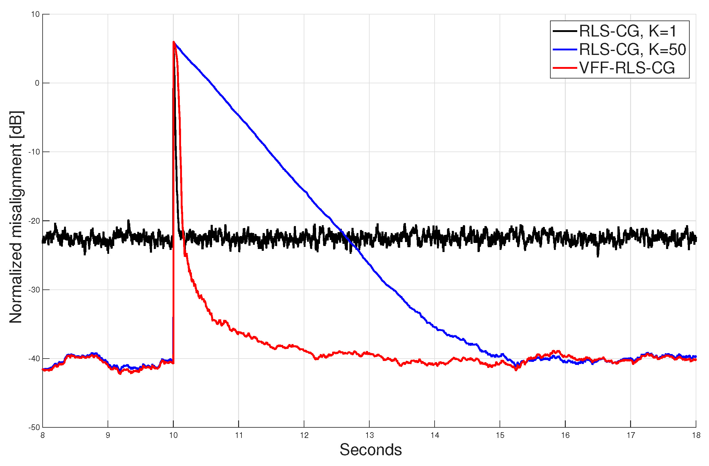
In the first scenario (Figure 1), the input signal is Gaussian noise, and the length of the echo path is set to $L=128$. Considering (16), the RLS-CG with $K=1$ is simulated as a reference method with high tracking capabilities. The echo path is changed after 10 s of simulation by switching the sign of all the corresponding coefficients.

It can be noticed that VFF-RLS-CG matches the tracking of RLS-CG with $K=1$ when the echo path changes. Moreover, at steady-state, the former adjusts the variable forgetting factor to increase its accuracy. The performances of the RLS-CG with $K=50$ are also added to the graphic in order to demonstrate the compromise made when the algorithm has a forgetting factor chosen to match the performances of VFF-RLS-CG at steady-state. When the tracking situation occurs, the RLS-CG with $K=50$ identifies the new impulse response much slower than the RLS-CG with $K=1$, namely VFF-RLS-CG. The scenario shows that a constant value for $\lambda$ cannot ensure the maximum efficiency for tracking and steady-state accuracy at the same time.

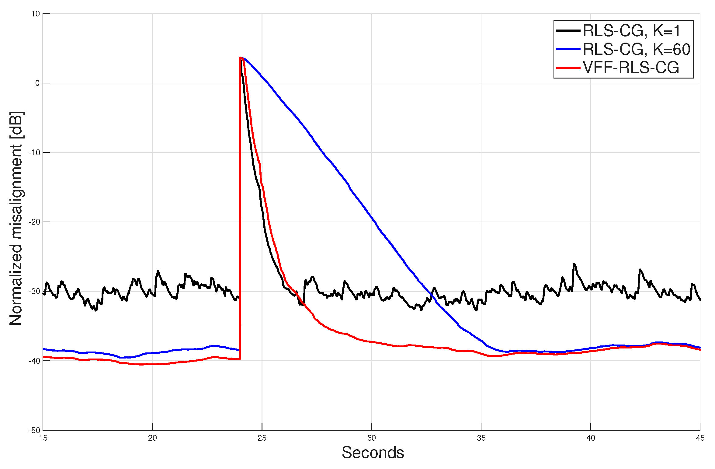
A tracking scenario is also simulated using (as input signal) a Gaussian noise filtered through an autoregressive system with a single pole [AR(1)] with the value $0.99$. The length of the echo path is set to $L=256$, and a tracking situation is obtained by shifting its coefficients by 25 positions at time index 24 s. VFF-RLS-CG is again compared with the RLS-CG with $K=1$, with respect to an RLS-CG variant matching VFF-RLS-CG accuracy at steady-state ($K=60$). The results in Figure 2 show that the VFF reproduces the desired behavior of its counterparts without manifesting their weaknesses. When the unknown impulse response changes, the value of $\lambda \left(n\right)$ decreases, and the tracking capabilities increase to match the performances of the RLS-CG with the lower forgetting factor value. Moreover, at steady-state, VFF-RLS-CG increases the value of $\lambda \left(n\right)$ to ensure improved accuracy. The classical compromise made when choosing the constant value of $\lambda$ is eliminated. The proposed algorithm demonstrates the mentioned performances despite working with a highly correlated input signal (see the approximation employed in Section 3).

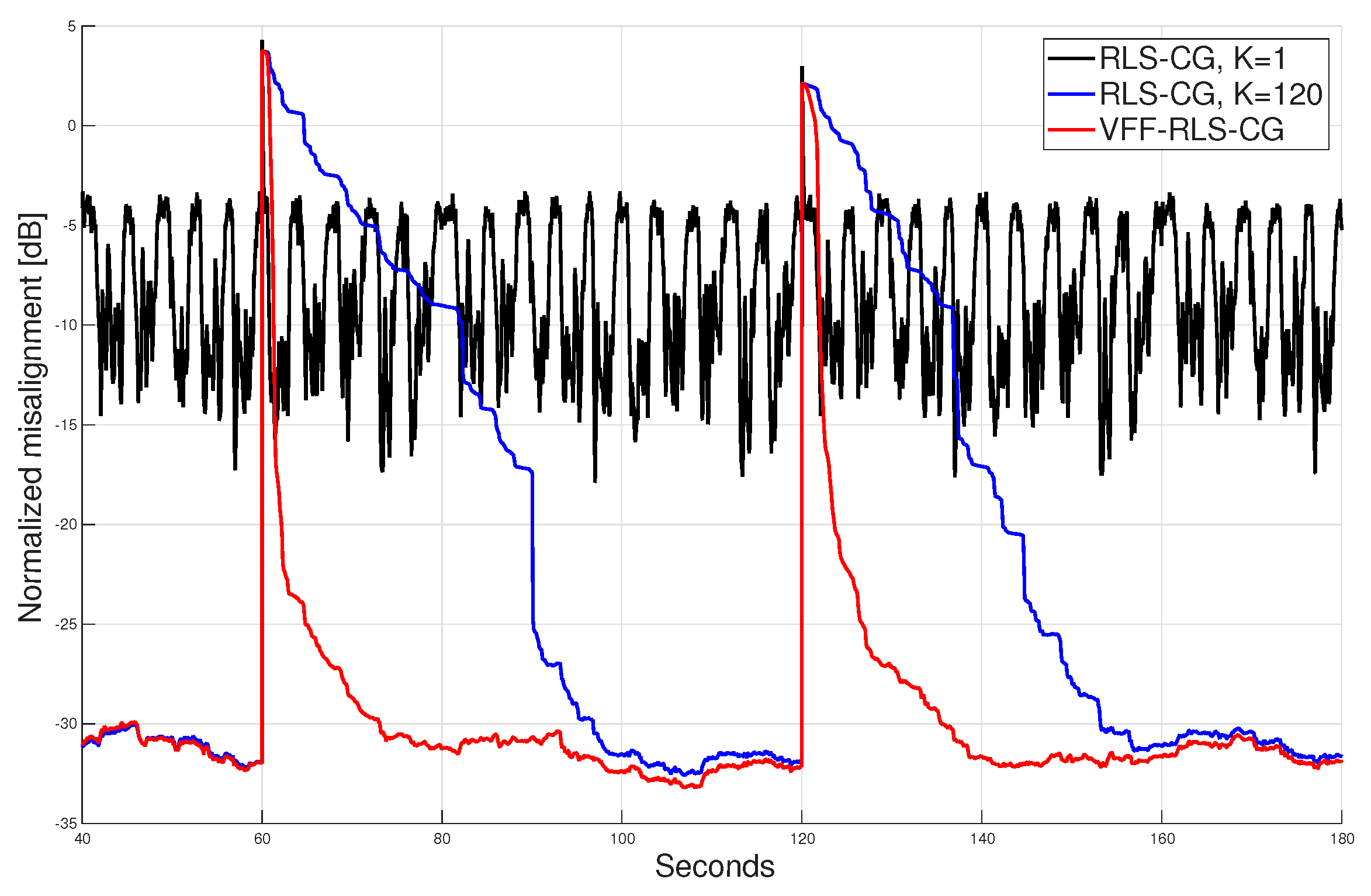
In the third experiment, the correlation properties of the input signal are further considered by employing a speech sequence, which is also non-stationary [31]. The length of the unknown system is set to a value closer to that in scenarios associated with real-world acoustic applications ($L=512$). The unknown system is changed twice by using both methods employed in the previous simulations. Tracking is expected to be more challenging for any adaptive algorithm performing AEC.

Furthermore, in order to demonstrate the practical value of VFF-RLS-CG, the variance in the noise signal, $v\left(n\right)$, is estimated in real time using an exponential window similar to (31) by determining ${\sigma }_v^2\left(n\right)$ as

$$\begin{array}{c}\hfill {\sigma }_v^2\left(n\right)=\beta {\sigma }_v^2(n-1)+(1-\beta )e^2\left(n\right),\end{array}$$

(34)

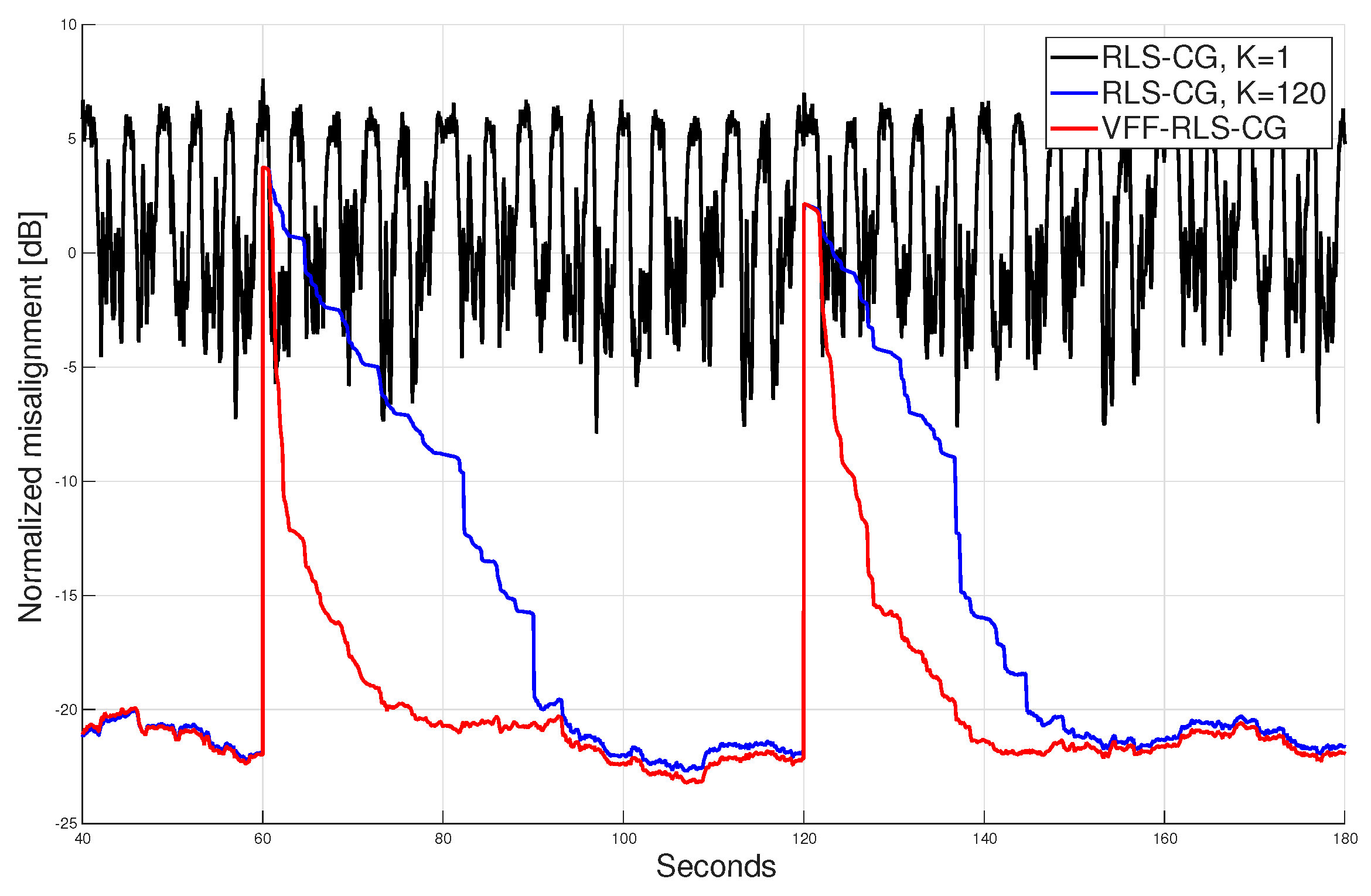
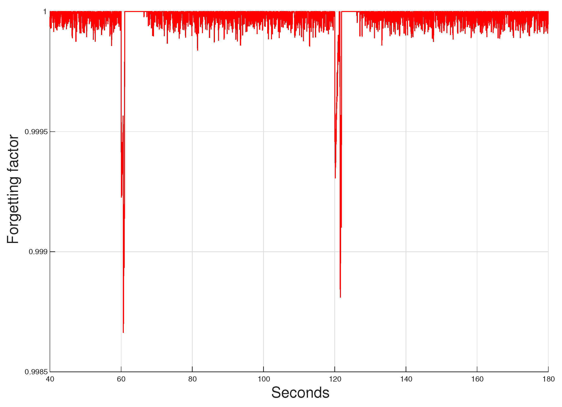
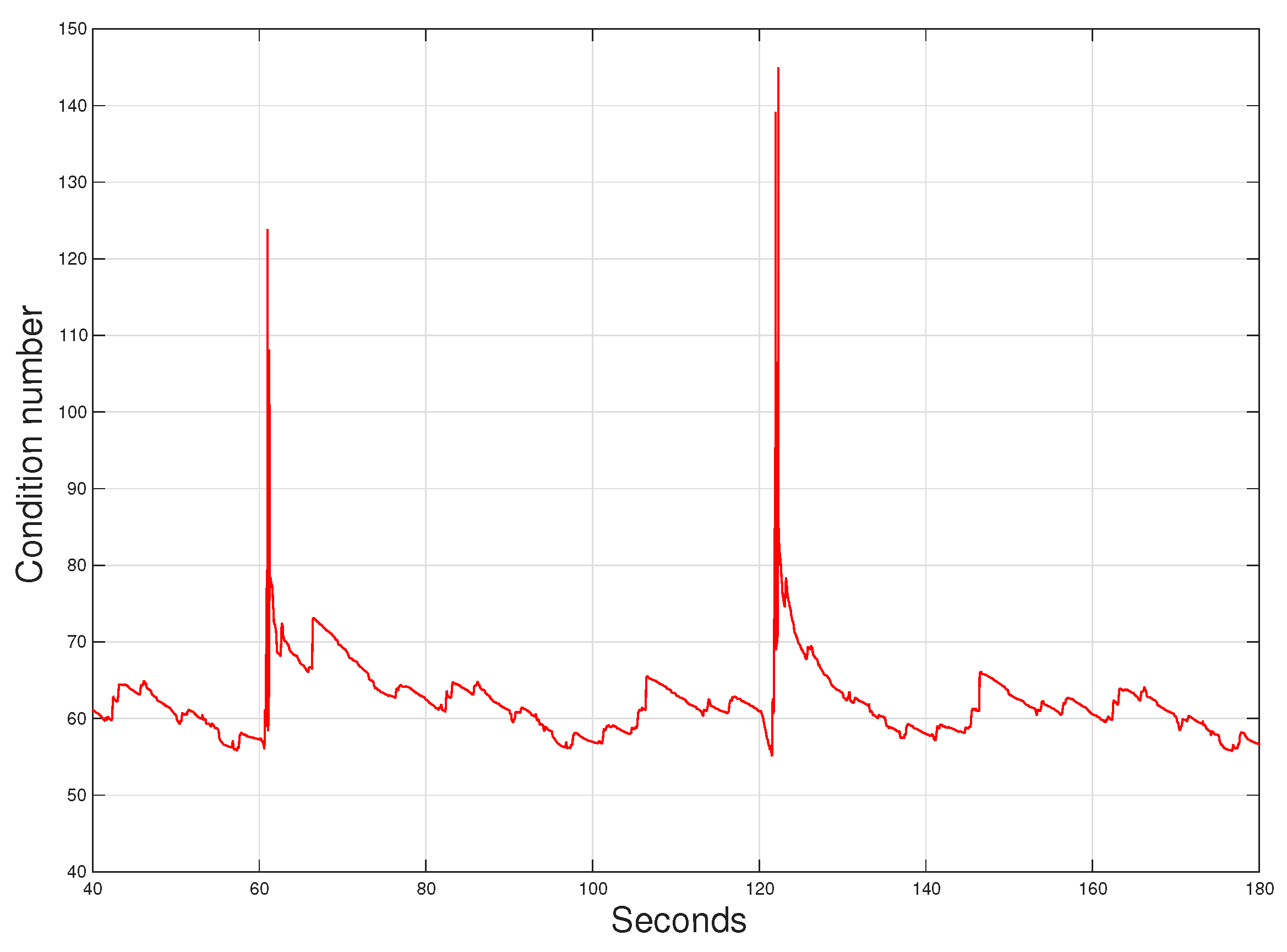
with $\beta >\gamma$ ensuring that the value of ${\sigma }_v^2\left(n\right)$ is estimated using a longer exponential window, with respect to the case of ${\sigma }_e^2\left(n\right)$ [22,30]. The corresponding results are displayed in Figure 3, while the evolution of the forgetting factor associated with VFF-RLS-CG is shown in Figure 4. Additionally, the variation in the condition number corresponding to the covariance matrix $\mathbf{R}\left(n\right)$ is depicted in Figure 5, showing a stable behavior [32].

It can be noticed that VFF-RLS-CG can match the tracking performances of the RLS-CG variant with reduced memory and the steady-state accuracy of the RLS-CG with the higher memory set through a higher value of $\lambda$. The evolution of the variable $\lambda \left(n\right)$ shown in Figure 4 indicates the corresponding values decreasing in the intervals in which the tracking should be optimized. When convergence is achieved, the values of $\lambda \left(n\right)$ oscillate closer to the value 1. In this context, we should outline that the additional control of $\alpha \left(n\right)$ from Equation (32) avoids numerical issues (which should be considered in practical implementations), while it could disrupt the continuity of the solution. Nevertheless, this truncation does not affect the algorithm’s performance, as indicated in Figure 4. As can be noticed, the lower limit (zero) is never reached, while the upper bound (one) is used for a short period of time, especially after the system changes (i.e., for tracking situations). However, using the maximum value of the forgetting factor does not affect but it rather favors the stability of the algorithm, which is a well-known conclusion reported in many convergence analyses of RLS-type algorithms [1,4,5].

The previous experiment was repeated in Figure 6 for ENR = 10 dB. Similar conclusions can be outlined. The RLS-CG variant with low (constant) $\lambda$ demonstrates poor performances, while the version with the higher constant forgetting factor demonstrates good accuracy at steady-state, with degradation in terms of tracking. However, VFF-RLS-CG demonstrates high tracking capabilities and the capacity to adjust its $\lambda \left(n\right)$ in order to attain accurate steady-state performances.

6. Conclusions

This paper presented a combination between the RLS adaptive algorithm and the CG LSM with the capability of adjusting its memory by computing the associated forgetting factor at every adaptive filter’s iteration. VFF-RLS-CG decreases the value of $\lambda \left(n\right)$ when the unknown impulse response is changed, and it increases $\lambda \left(n\right)$ at steady-state. The VFF part of the algorithm adds reduced arithmetical effort in terms of multiplications and divisions and eliminates the compromise made when choosing a fixed value for $\lambda$ in classical RLS methods.

Simulations demonstrated the validity of the theoretical VFF-RLS-CG model. It can match the performances of the RLS-CG optimized for tracking situations and for steady-state portions. The algorithm is numerically stable and suitable for working with AEC configurations and with highly correlated signals.

Future works will focus on studying low-complexity VFF-RLS-LSM variants by combining RLS with dichotomous coordinate descent (DCD) iterations [6,7,8]. The main benefits will be achieving the advantages of RLS methods with the VFF approach and obtaining a VFF-RLS-DCD version with an overall arithmetic complexity proportional to the adaptive filter’s length, which is attractive for real-time signal processing platforms.