Applications of the Kalman Filter in Physical Processes: A Review

Abstract

This article outlines various specialized adaptations of the Kalman Filter designed to address specific estimation challenges across different domains of Physics. The work demonstrates the significant potential of the Kalman filter to enhance the accuracy and reliability of measurements in Physics, providing robust, real-time, and adaptive estimation capabilities. The paper starts with an extensive introduction to the core of the Kalman filter. A clear description of the different filter categories follows, along with the conditions under which each is applied. Various Kalman filter variants address nonlinear, adaptive, continuous-time, large-scale, and uncertain systems. These include the Extended and Unscented Kalman Filters for nonlinear estimation, Adaptive and Kalman–Bucy filters for changing or continuous dynamics, and Ensemble or Schmidt–Kalman filters for large or reduced-order systems. Robust, Cubature, Probabilistic, and Particle Kalman filters further improve performance under outliers, strong nonlinearities, and non-Gaussian uncertainty. To illustrate the practical relevance, detailed applications in Physics are discussed, including thermodynamics, electromagnetism, high-energy physics, quantum physics, and astrophysics, highlighting how Kalman filtering enhances both predictive accuracy and measurement-informed decision-making.

1. Introduction

The estimation and prediction of dynamical systems in the presence of uncertainty constitute a central challenge in physics. In many physical processes, the quantities of interest cannot be directly observed and must instead be inferred from incomplete, noisy, or indirect measurements. These limitations arise from fundamental stochasticity, model simplifications, measurement imperfections, or constraints on experimental access. Kalman filtering provides a mathematically rigorous and computationally efficient framework to address this challenge by combining physical models with observational data in a statistically optimal manner.

Originally introduced by Rudolf E. Kalman as a recursive solution to the linear discrete-data filtering problem [1], the Kalman filter has since become a cornerstone of estimation theory. Its predictor–corrector structure enables the continuous refinement of state estimates by balancing model-based predictions against incoming measurements, while explicitly accounting for uncertainty. Beyond its classical derivation, the Kalman filter can also be interpreted through Bayesian inference and maximum likelihood estimation, highlighting its role as a fundamental information-extraction mechanism rather than a purely numerical algorithm [2,3,4].

In physics, uncertainty is not merely a technical inconvenience but an intrinsic feature of many systems. From macroscopic thermo-fluid flows governed by approximate closure models to electromagnetic and particle systems subject to sparse sensing, and down to quantum and stochastic processes constrained by measurement back-action, the accurate inference of system states is often the limiting factor in prediction, control, and interpretation. Kalman filtering addresses this limitation by providing a unified estimation framework that remains applicable across scales, physical regimes, and levels of model fidelity [5,6,7].

This review focuses on the role of Kalman-based methodologies as enabling tools for state estimation in diverse areas of physics. Rather than presenting a purely algorithmic overview, the emphasis is placed on how Kalman filtering interacts with physical modeling assumptions, uncertainty sources, and domain-specific constraints. The filter is examined not only as an estimator but also as a mechanism that reveals structure in physical systems by optimally integrating dynamics, measurements, and noise.

At the core of non-linear filtering theory lies the Kushner equation (also known as the Kushner–Stratonovich equation), which provides a rigorous mathematical framework for the evolution of the conditional probability density of a stochastic dynamical system’s state, given a stream of noisy observations [8,9,10,11,12]. While the classic Kalman Filter provides the exact solution for linear Gaussian systems, the Kushner equation generalizes this principle to non-linear dynamics, serving as the theoretical benchmark for the many Kalman-type approximations and generalizations discussed in this review.

The paper is organized as follows. Section 2 presents the theoretical foundations of the Kalman filter, including its formulation, assumptions, and mathematical structure [5,6]. Section 3 reviews the main classes and extensions of Kalman filtering, highlighting how modifications such as nonlinear, extended, and unscented variants address departures from idealized linear Gaussian conditions [13,14,15,16,17,18,19,20,21,22,23,24,25,26,27,28,29,30,31,32,33,34,35,36,37,38,39,40,41,42,43,44,45,46,47,48,49,50,51,52,53,54,55,56,57]. While this review specifically focuses on these core developments (Extended Kalman Filter (EKF) and Unscented Kalman Filter (UKF)), it is worth noting that the broader family of Kalman filters extends to advanced data assimilation techniques for coherent structures and complex non-linear phenomena [58]. From Section 4 onward, the focus shifts to applications in physics, illustrating how Kalman-based estimation strategies are adapted to distinct physical contexts.

Section 4 examines thermodynamic systems, where uncertainty, partial observability, and strong coupling between physical variables are inherent features [59,60,61,62,63,64,65,66,67,68,69,70,71,72,73,74,75,76]. Two complementary applications are reviewed: Kalman-based data assimilation in large-scale thermo-fluid dynamics, and Kalman–Bucy filtering in stochastic thermodynamics with measurement and feedback, revealing deep connections between estimation, information, and energetic performance. Section 5 addresses electromagnetic systems, including real-time inversion and field estimation from sparse measurements, demonstrating how Kalman filtering enables spatially extended inference from limited data [77,78,79,80,81,82,83,84,85,86,87,88,89,90,91,92,93,94,95]. Section 6 focuses on high-energy physics, where advanced Kalman filter variants improve the tracking of subatomic particles under nonlinear dynamics and severe measurement noise [96,97,98,99,100,101,102,103,104,105,106,107,108,109,110,111]. Section 7 explores quantum-scale applications, highlighting the use of Kalman filtering in atomic magnetometry and the formulation of quantum extended Kalman filters for open quantum systems [112,113,114,115,116,117,118,119,120,121,122,123,124,125,126,127,128,129,130]. Finally, Section 8 reviews applications in astrophysics, including interferometric control and particle tracking in large-scale detection experiments [131,132,133,134,135,136,137,138,139,140,141].

By examining these applications within a unified estimation framework, this review highlights how Kalman filtering serves as a cross-disciplinary bridge between physical modeling, uncertainty quantification, and information processing. Across all domains considered, a common theme emerges: Kalman-based approaches enable physically consistent, uncertainty-aware inference that enhances both predictive accuracy and interpretability. The conclusions summarize these insights and outline perspectives for future developments in Kalman-based methods for complex physical systems.

Despite its long-standing history, the Kalman filter remains a cornerstone of contemporary research, continuously evolving to address the complexities of modern technological applications. Recent literature highlights a significant shift toward hybridizing the filter with artificial intelligence and data-driven designs [142,143], while addressing challenges such as non-Gaussian measurement noises [144] and outlier robustness through kernel density estimation [145]. Furthermore, cutting-edge variations like the Inverse Unscented Kalman Filter [146], advanced adaptive schemes for structural identification [147,148], and its integration into autonomous UAV systems [149] demonstrate that the framework is being actively refined to meet the demands of high-dimensional, real-time sensing.

2. The Kalman Filter

2.1. Mean Squared Error

Many signals can be described in the following way:

$$y_k=a_k{x}_k+n_k$$

(1)

where $y_k$ is the time-dependent observed signal, $a_k$ is a gain term, $x_k$ is the information bearing signal and $n_k$ is the additive noise.

The overall objective is to estimate $x_k$. The difference between the estimate of ${\widehat{x}}_k$ and $x_k$ itself is termed the error:

$$f\left(e_k\right)=(x_k-{\widehat{x}}_k)$$

(2)

The particular shape of $f\left(e_k\right)$ is dependent upon the application, however it should be both positive and monotonically increasing. An error function that exhibits these characteristics is the squared error function:

$$f\left(e_k\right)={(x_k-{\widehat{x}}_k)}^2$$

(3)

Since it is necessary to consider the ability of the filter to predict many data over a period of time, a more meaningful statistical metric is the loss function $L$, defined as the expected value of the error function:

$$L=E\left(f\left(e_k\right)\right)$$

(4)

This results in the mean squared error (MSE) function:

$$ϵ\left(t\right)=E\left({e_k}^2\right)$$

(5)

2.2. Maximum Likelihood

The above derivation of mean squared error, although intuitive, is somewhat heuristic. A more rigorous derivation can be developed using maximum likelihood statistics. This is achieved by redefining the goal of the filter as finding the $\widehat{x}$ that maximises the probability or likelihood of y. That is:

$$\mathrm{m}\mathrm{a}\mathrm{x}\left[P\left(y\right|{\widehat{x}}_k\right)]$$

(6)

Assuming that the additive random noise is Gaussian-distributed with a standard deviation of ${\sigma }_k$ gives:

$$[P\left(y\right|{\widehat{x}}_k)]=K_k\mathrm{e}\mathrm{x}\mathrm{p}\left(-{\displaystyle \frac{{(y_k-a_k{\widehat{x}}_k)}^2}{{2{\sigma }_k}^2}}\right)$$

(7)

where $K_k={\displaystyle \frac{1}{\sqrt{2\pi }{\sigma }_k}}$ is the normalization constant. Consequently, the maximum likelihood function, denoted as $\mathcal{L}$, is rigorously defined as:

$$\mathcal{L}=\prod _k{K}_{k}exp\left(-{\displaystyle \frac{{(y_k-a_k{\widehat{x}}_k)}^2}{{2{\sigma }_k}^2}}\right)$$

(8)

Assuming a stationary noise process where the error covariance remains constant over time (${\sigma }_k=const$), it leads to:

$$\begin{array}{c}\log P\left(y\right|\widehat{x})={\displaystyle \sum _k}\mathrm{l}\mathrm{o}\mathrm{g}{K}_k+{\displaystyle \sum _k}\left({\displaystyle \frac{{-\left(y_k-a_k{\widehat{x}}_k\right)}^2}{{2{\sigma }_k}^2}}\right)\Rightarrow \\ \log P\left(y\right|\widehat{x})=-{\sum }_k\left({\displaystyle \frac{{\left(y_k-a_k{\widehat{x}}_k\right)}^2}{{2{\sigma }_k}^2}}\right)+constant\end{array}$$

(9)

The driving function of Equation (9) is the MSE, which may be maximised by the variation of ${\widehat{x}}_k$. Therefore, the mean squared error function is applicable when the expected variation of $y_k$ is best modelled as a Gaussian distribution. In such a case, the MSE serves to provide the value of ${\widehat{x}}_k$ that maximises the likelihood of the signal $y_k$.

2.3. Subsection Kalman Filter State Space Derivation

Before discussing the Kalman filter, the work of Norbert Wiener should first be acknowledged. Wiener described an optimal finite impulse response (FIR) filter in the mean squared error sense. His solution will not be discussed here even though it has much in common with the Kalman filter. Suffice to say that his solution uses both the autocorrelation and the cross-correlation of the received signal with the original data, to derive an impulse response for the filter (the filter coefficients).

Kalman’s approach to the optimal minimum mean square error (MSE) filter offers several advantages over the Wiener filter. Unlike the Wiener filter, which requires determining the impulse response—often challenging for numerical computations, Kalman’s filter uses state space techniques. This flexibility allows it to function as a smoother, filter, or predictor. Its predictive capability has made the Kalman filter particularly valuable in various tracking and navigation applications. Additionally, defining the filter with state space methods simplifies its implementation in the discrete domain, contributing to its popularity and widespread use.

2.3.1. The Problem Solved by the Linear Kalman Filter

The preceding derivation utilized scalar notations to intuitively introduce the core estimation principles, physical systems are generally multi-dimensional. To account for coupled dynamics and multiple variables, the scalar framework is now extended to a multi-variable state-space representation. Consequently, the state and measurement equations are generalized into the following vector-matrix form.

We want to know the value of a variable $x_k$ (in general a vector) as the time $t_k$ is evolving. The variable $x_k$ describes, in general, a physical system or phenomenon that is evolving in time. We have available two different sources of information for $x_k$

• The first source of information is the way that the system is physically governed and evolving described by the prediction matrix $A$ by means of the prediction equation

$$x_{k+1}=A{x}_k+w_k$$

(10)

where $x_k$ is the state vector of the prediction process of dimensions $\left(\mathrm{n}\mathrm{x}1\right)$ at time $t_k$. $A$ is the state transition (or prediction) matrix of the process transforming the state $x_k$ at time $t_k$ to the state $x_{k+1}$ at time $t_{k+1}$, and is assumed stationary over time. The dimensions of $A$ are $\left(\mathrm{n}✕\mathrm{m}\right).$ Finally, $w_k$ is the associated white process noise with known covariance, and dimensions $\left(\mathrm{n}✕1\right).$

b.

The second source of information is based on the observation process model, i.e., at time $t_k$ we acquire a measurement

$$z_k=H{x}_k+u_k$$

(11)

where $z_k$ is the actual measurement of $x_k$ at time $t_k$, (dimensions $m\times 1$). $H$ is the noiseless connection between the state vector $x_k$ and the measurement vector $z_k$ and is assumed stationary over time $\left(\mathrm{m}\mathrm{x}\mathrm{n}\right)$, while $u_k$ is the associated measurement error. This is again assumed to be a white noise process with known covariance and has zero cross-correlation with the process noise (dimensions $\mathrm{m}\times 1$). The observation process otherwise called estimation process is employed to acquire complementary information for $x_k$ by means of the measurement matrix $H$ and assign it onto $z_k$. The measure $z_k-H{x}_k$ is the additional (improved) information we obtained from the measurement to better estimate $x_k$.

It is very important to mention that we can consider the variable-state $x_k$ as being Normal distributed with mean ${\widehat{x}}_k$ and covariance $P_k$, i.e.,

$$x_k ~ N({\widehat{x}}_k, P_k)$$

(12)

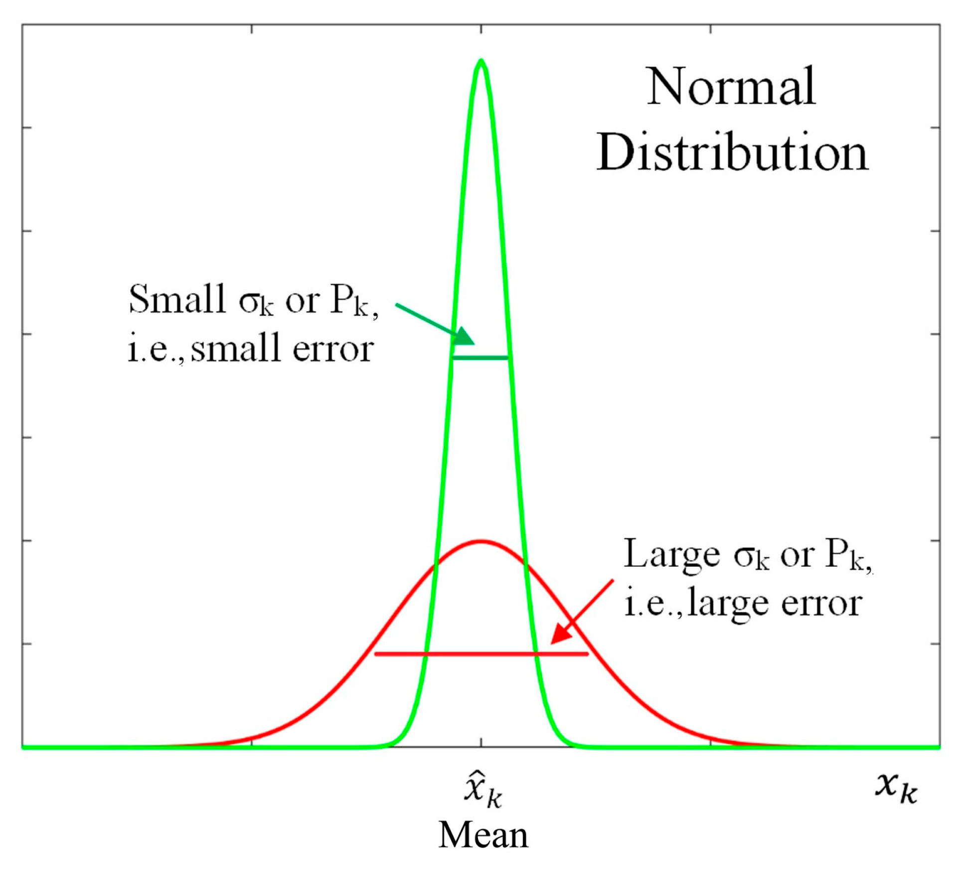
as shown in Figure 1.

For the minimisation of the MSE to yield the optimal filter it must be possible to correctly model the system errors using Gaussian distributions. The covariances of the two noise models are assumed stationary over time and are given by:

$$Q=E\left[w_k{w_k}^T\right]$$

(13)

$$R=E\left[u_k{u_k}^T\right]$$

(14)

The mean squared error is given by Equation (5). This is equivalent to:

$$E\left[e_k{e_k}^T\right]=P_k$$

(15)

where $P_k$ is the error covariance matrix ($nxn$) at time $t_k$.

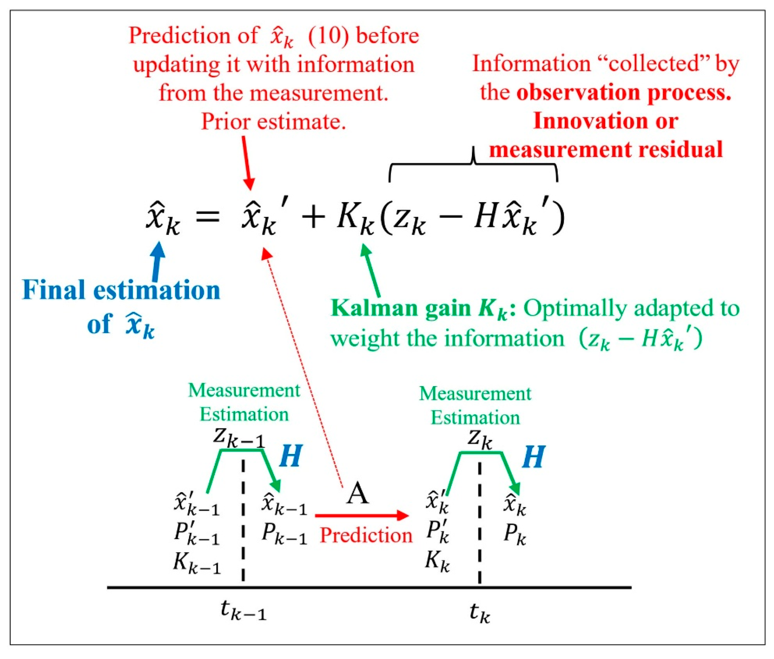
To intuitively understand how information is manipulated we need to dwell for a moment in symbolisms $x_k$, ${\widehat{x}}_k$ and ${{\widehat{x}}_k}^{\prime }$. A key point to understand the whole process of the linear Kalman filter is the idea to “improve” the prediction of ${\widehat{x}}_k$ obtained from Equation (10) just before “presenting” it and symbolizing this quantity as ${{\widehat{x}}_k}^{\prime }$ [7]. Figure 2 presents intuitively this procedure. The improvement of ${{\widehat{x}}_k}^{\prime }$ (obtained from Equation (10)) is achieved by correcting this quantity with information “collected” by the observation process Equation (11) modelled in the form $z_k-H{x}_k$ and weighted by the Kalman gain $K_k$:

$${\widehat{x}}_k={{\widehat{x}}_k}^{\prime }+K_k(z_k-H{{\widehat{x}}_k}^{\prime })$$

(16)

The Kalman gain $K_k$ is continuously adapted with time to optimally weight the information $z_k-H{{\widehat{x}}_k}^{\prime }$ (Innovation or measurement residual).

2.3.2. Steps to Follow to Complete the Procedure

In the following subsections, we must:

• Evaluate the prior estimate ${P_k}^{\prime }$ of $P_k$.
• This estimate contains the Kalman gain $K_k$, which is to be evaluated so that it is optimal in the sense that it optimally weights the correction of the Innovation or Measurement Residual in Equation (16).
• Determine the final form of $P_k$.
• Describe the whole Kalman Estimation Filter procedure.

2.3.3. The Prior Estimate ${P_k}^{\prime }$ of $P_k$

The error covariance matrix $P_k$ connected to the material expressed by Equation (2) to Equation (5) is as follows:

$$P_k=E\left[e_k{e_k}^T\right]=E\left[\right(x_k-{\widehat{x}}_k\left){(x_k-{\widehat{x}}_k)}^T\right]$$

(17)

Assuming the prior estimate of ${\widehat{x}}_k$ is called ${{\widehat{x}}_k}^{\prime }$ and was gained by knowledge of the system $A$ (see Figure 2), it is possible to write an update equation for the new estimate, combining the old estimate with measurement data. Thus, substituting Equation (11) into Equation (16) and given that, as mentioned previously, the term $z_k-H{{\widehat{x}}_k}^{\prime }$ is known as the innovation or measurement residual:

$$i_k=(z_k-H{{\widehat{x}}_k}^{\prime })$$

(18)

the following is obtained:

$${\widehat{x}}_k={{\widehat{x}}_k}^{\prime }+K_k(H{x}_k+u_k-H{{\widehat{x}}_k}^{\prime })$$

(19)

The error from Equation (2) is written based on Equation (19):

$$\begin{array}{c}{e}_k=x_k-{\widehat{x}}_k\Rightarrow \\ e_k=x_k-{[{\widehat{x}}_k}^{\prime }+K_k(H{x}_k+u_k-H{{\widehat{x}}_k}^{\prime })]\Rightarrow \\ e_k=x_k-[{{\widehat{x}}_k}^{\prime }+K_{k}H(x_k-{{\widehat{x}}_k}^{\prime })+K_k{u}_k]\Rightarrow \\ e_k=x_k-{{\widehat{x}}_k}^{\prime }-K_{k}H\left(x_k-{{\widehat{x}}_k}^{\prime }\right)-K_k{u}_k\Rightarrow \\ e_k=(I-K_{k}H)\left(x_k-{{\widehat{x}}_k}^{\prime }\right) -K_k{u}_k\end{array}$$

(20)

where I is the identity matrix.

Substitution of Equation (20) into Equation (17) gives the error covariance matrix $P_k$:

$$\begin{array}{cc}\hfill P_k& =E\left[e_k{e_k}^T\right]\hfill \\ & =E\left[\left[\right(I-K_{k}H\left)\right(x_k-{{\widehat{x}}_k}^{\prime })-K_k{u}_k)]{\left[\right(I-K_{k}H\left)\right(x_k-{{\widehat{x}}_k}^{\prime })-K_k{u}_k]}^T\right]\hfill \\ \hfill P_k& =E\left[\left[\left(I-K_{k}H\right)\left(x_k-{{\widehat{x}}_k}^{\prime }\right)\right]{\left[\left(I-K_{k}H\right)\left(x_k-{{\widehat{x}}_k}^{\prime }\right)\right]}^T\right]\hfill \\ & -E\left[\left(I-K_{k}H\right)\left(x_k-{{\widehat{x}}_k}^{\prime }\right){{(K}_k{u}_k)}^T\right]\hfill \\ & -E\left[K_k{u}_k\right[{\left(x_k-{{\widehat{x}}_k}^{\prime }\right)}^T{\left(I-K_{k}H\right)]}^T]\hfill \\ & +E\left[K_k{u}_k\right[K_k{u_k]}^T]\hfill \end{array}$$

(21)

In this quantity the second and third terms are each equal to zero since the error of the prior estimate $x_k-{{\widehat{x}}_k}^{\prime }$ is uncorrelated with the measurement noise $u_k$. Accordingly

$$\begin{array}{cc}\hfill P_k& =E\left[\left(I-K_{k}H\right)\left(x_k-{{\widehat{x}}_k}^{\prime }\right){\left(x_k-{{\widehat{x}}_k}^{\prime }\right)}^T{\left(I-K_{k}H\right)}^T\right]+E\left[K_k{u}_k{u}_k^T{K}_k^T\right]\hfill \\ & =\left(I-K_{k}H\right)E\left[\left(x_k-{{\widehat{x}}_k}^{\prime }\right){\left(x_k-{{\widehat{x}}_k}^{\prime }\right)}^T\right]{\left(I-K_{k}H\right)}^T+K_{k}E\left[u_k{u_k}^T\right]{K_k}^T\hfill \end{array}$$

(22)

and thus, having in mind Equations (14) and (15), we obtain the error covariance update equation:

$$P_k=\left(I-K_{k}H\right){P_k}^{\prime }{\left(I-K_{k}H\right)}^T+K_{k}R{K_k}^T$$

(23)

where ${P_k}^{\prime }$ is the prior estimate of $P_k$.

2.3.4. Evaluation of the Kalman Gain $K_k$

The diagonal of the error covariance matrix contains the mean squared errors as derived by:

$$P_{kk}=Cov\left(e_k\right)=E\left[e_k{e_k}^T\right]$$

(24)

If $e_k=\left[\begin{array}{c}{e}_{k-1}\\ e_k\\ e_{k+1}\end{array}\right]$ and ${e_k}^T=\left[\begin{array}{ccc}{e}_{k-1}& e_k& e_{k+1}\end{array}\right]$,

$$P_{kk}=\left[\begin{array}{ccc}{E[e}_{k-1}{e}_{k-1}]& {E[e}_{k-1}{e}_k]& {E[e}_{k-1}{e}_{k+1}]\\ E\left[e_k{e}_{k-1}\right]& {E[e}_k{e}_k]& {E[e_{k}e}_{k+1}]\\ {E[e_{k+1}e}_{k-1}]& {E[e_{k+1}e}_k]& {E[e}_{k+1}{e}_{k+1}]\end{array}\right]$$

(25)

The sum of the diagonal elements of a matrix is called its trace. In the case of the error covariance matrix the trace is the sum of the mean squared errors. Therefore, the mean squared error may be minimised by minimising the trace of $P_k$, which, in turn, will minimise the trace of $P_{kk}$:

$$\begin{array}{cc}\hfill tr\left(P_{kk}\right)& =tr\left({E[e}_{k-1}{e}_{k-1}\right]+tr{E[e}_k{e}_k]+tr{E[e}_{k+1}{e}_{k+1}])\hfill \\ & =E\left[{‖e_{k-1}‖}^2\right]+E\left[{‖e_k‖}^2\right]+E\left[{‖e_{k+1}‖}^2\right]\hfill \end{array}$$

(26)

The MSE is the sum divided by the number of factors and becomes minimum when $tr\left(P_k\right)$ is minimized, means also when $tr\left(P_{kk}\right)$ becomes minimum.

From Equation (23) we have:

$$\begin{array}{c}{P}_k=\left(I-K_{k}H\right){P_k}^{\prime }{\left(I-K_{k}H\right)}^T+K_{k}R{K_k}^T\hfill \\ P_k={P_k}^{\prime }-K_{k}H{P_k}^{\prime }-{P_k}^{\prime }{H}^T{K}_k^T+K_k{{(H{{P_k}^{\prime }H}^T+R)K}_k}^T\hfill \end{array}$$

(27)

The trace of $P_k$ is first differentiated with respect to $K_k$ and the result set to zero to find the conditions of this minimum.

Note that:

• Covariances of real processes are symmetric;
• Therefore, they are equal to their transpose;
• Therefore, the trace of a symmetric matrix is equal to the trace of its transpose; therefore, it can be written as:

$$tr\left(P_k\right)=tr\left({P_k}^{\prime }\right)-tr\left(K_{k}H{P_k}^{\prime }\right)-tr\left({K_k}^T{H}^T{P_k}^{\prime }\right)+tr\left[K_k{{(H{P_k}^{\prime }{H}^T+R)K}_k}^T\right]$$

(28)

Differentiating with respect to $K_k$ we have:

$${\displaystyle \frac{dT\left[P_k\right]}{d{K}_k}}=-2{\left(H{P_k}^{\prime }\right)}^T+2K_k(H{P_k}^{\prime }{H}^T+R)$$

(29)

Setting the derivative equal to zero and rearranging gives:

$${\left(H{P_k}^{\prime }\right)}^T=K_k(H{P_k}^{\prime }{H}^T+R)$$

(30)

Now solving for $K_k$ and noting that the matrix ${P_k}^{\prime }$ is symmetric, we have:

$$K_k{={P_k}^{\prime }H}^T {(H{P_k}^{\prime }{H}^T+R)}^{-1}$$

(31)

Equation (31) is the Kalman gain equation.

2.3.5. Final Form of the Error Covariance Matrix $P_k$

Taking into consideration that the innovation $i_k=(z_k-H{{\widehat{x}}_k}^{\prime })$ from (19) has an associated measurement prediction covariance defined as

$$S_k=H{P_k}^{\prime }{H}^T+R$$

which is symmetric, and substituting Equation (27) gives:

$$\begin{array}{cc}\hfill P_k& ={P_k}^{\prime }-{{K_{k}HP}_k}^{\prime }-{P_k}^{\prime }{H}^T{K_k}^T+K_k{S}_k{K_k}^T\hfill \\ & ={P_k}^{\prime }-{P_k}^{\prime }{H}^T{\left(S_k\right)}^{-1}H{P_k}^{\prime }\hfill \\ & -{P_k}^{\prime }{H}^T{{[{P_k}^{\prime }H}^T{\left(S_k\right)}^{-1}]}^T\hfill \\ & +\left[{{P_k}^{\prime }H}^T{\left(S_k\right)}^{-1}\right]S_k[{P_k}^{\prime }{H}^T{{[{P_k}^{\prime }H}^T{\left(S_k\right)}^{-1}]}^T\hfill \\ & ={P_k}^{\prime }-{P_k}^{\prime }{H}^T{S_k}^{-1}H{P_k}^{\prime }-{P_k}^{\prime }{H}^T{{[{P_k}^{\prime }H}^T{(S_k}^{-1}\left)\right]}^T\hfill \\ & +\left[{{P_k}^{\prime }H}^T{(S_k}^{-1})\right]S_k[{P_k}^{\prime }{H}^T{{[{P_k}^{\prime }H}^T{(S_k}^{-1}\left)\right]}^T\hfill \end{array}$$

We know that $P_k$ and $S_k$ are symmetric matrices, so:

$$\begin{array}{cc}\hfill P_k& ={P_k}^{\prime }-{P_k}^{\prime }{H}^T{S_k}^{-1}H{P_k}^{\prime }-{P_k}^{\prime }{H}^T{S_k}^{-1}H{P_k}^{\prime }+{P_k}^{\prime }{H}^T{S_k}^{-1}{S}_k{S_k}^{-1}H{P_k}^{\prime }\hfill \\ & ={P_k}^{\prime }-{{2P}_k}^{\prime }{H}^T{S_k}^{-1}H{P_k}^{\prime }+{P_k}^{\prime }{H}^T{S_k}^{-1}H{P_k}^{\prime }\hfill \\ & ={P_k}^{\prime }-{P_k}^{\prime }{H}^T{S_k}^{-1}H{P_k}^{\prime }\hfill \\ & ={P_k}^{\prime }-K_{k}H{P_k}^{\prime }\Rightarrow \hfill \\ \hfill P_k& =(I-K_{k}H){P_k}^{\prime }\hfill \end{array}$$

(32)

Equation (32) is the update equation for the error covariance matrix with optimal gain $K_k$.

2.4. Final Expression of Kalman Estimation Filter

The three Equations (16), (31) and (32) provide an estimate of the variable $x_k$. By employing Equation (10) the state projection is achieved:

$${{\widehat{x}}_{k+1}}^{\prime }=A{\widehat{x}}_k$$

(33)

To complete the recursion, it is necessary to find an equation that projects the error covariance matrix into the next time interval $k+1$. This is achieved by first forming an expression for the prior error:

$$\begin{array}{cc}\hfill {e_{k+1}}^{\prime }& =x_{k+1}-{{\widehat{x}}_{k+1}}^{\prime }\hfill \\ & =A{x}_k+w_k-A{\widehat{x}}_k\hfill \\ & =\left(A{x}_k+w_k\right)-A{\widehat{x}}_k\hfill \\ & =A{e}_k+w_k\hfill \end{array}$$

(34)

Extending Equation (15) to time $k+1$:

$$P_{k+1}^{\prime }=E\left[{e_{k+1}}^{\prime }{{e_{k+1}}^{\prime }}^T\right]=E\left[(A{e}_k{+w_k)\left(A{e}_k+w_k\right)}^T\right]$$

(35)

Note that $e_k$ and $w_k$ have zero cross-correlation because the noise $w_k$ accumulates between $k$ and $k+1$ whereas the error $e_k$ is the error up until time $k$. Therefore:

$$\begin{array}{c}{ P}_{k+1}^{\prime }=E\left[{e_{k+1}}^{\prime }{{e_{k+1}}^{\prime }}^T\right]=E\left[A{e}_k{\left(A{e}_k\right)}^T\right]+E\left[w_k{w_k}^T\right]=E\left[A{e}_k{e_k}^T{A}^T\right]+Q⟹\\ P_{k+1}^{\prime }=AE\left[e_k{e_k}^T\right]A^T+Q=A{P}_k{A}^T+Q\end{array}$$

(36)

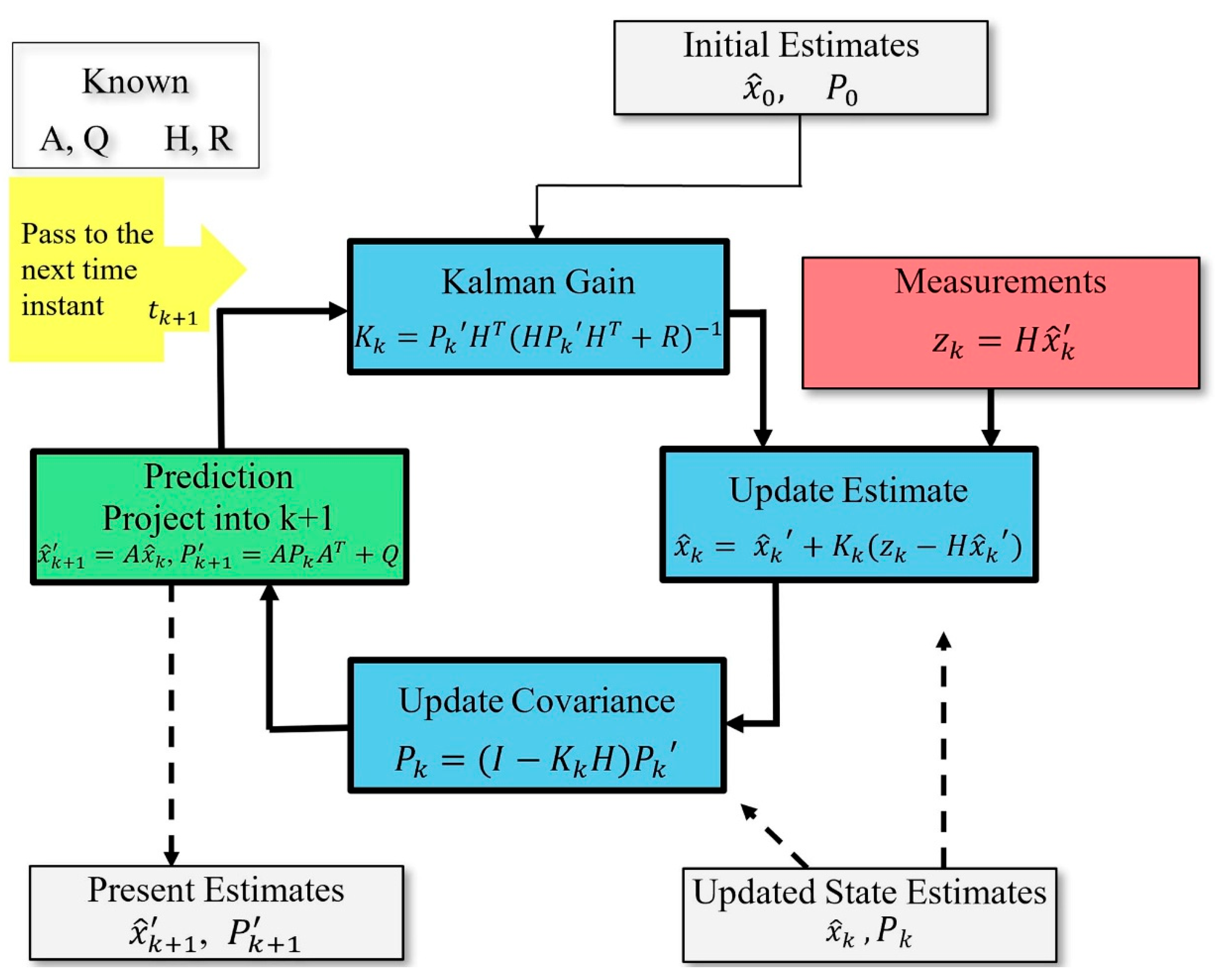
This completes the recursive filter. The algorithmic loop is summarised in the diagram of Figure 3.

3. The Evolution of the Kalman Filter

The Kalman Filter (KF) is a fundamental recursive algorithm designed for the optimal estimation of system states by synthesizing mathematical process models with stochastic physical measurements. In its fundamental form, the KF is tailored for linear systems; however, its inability to accurately track the behavior of more intricate and inherently non-linear systems has led to the development of several sophisticated variants. To bridge this gap, the EKF and the UKF were introduced, representing first-order and higher-order approximation strategies, respectively [15,16]. While the EKF remains a popular choice due to its relative simplicity in linearization, it often encounters convergence issues or implementation difficulties when faced with extreme system complexity. Consequently, the UKF emerged as a more robust alternative, offering a more robust framework for managing non-linearities without the degradation often seen in EKF performance.

Beyond standard non-linearity, the challenge of model uncertainty necessitated the design of the Robust Kalman Filter (RKF) for discrete-time systems. Furthermore, as modern engineering problems often involve high-dimensional state spaces, the Cubature Kalman Filter (CKF) was developed to provide a systematic and mathematically sound solution for non-linear filtering. A significant leap in estimation reliability has been achieved through the adoption of parallel filtering architectures. By assigning specific estimations to multiple filters operating in tandem, methods such as Multiple Model Adaptive Estimation (MMAE) and the Interacting Multiple Model (IMM) have become the industry standard for complex model sets [13].

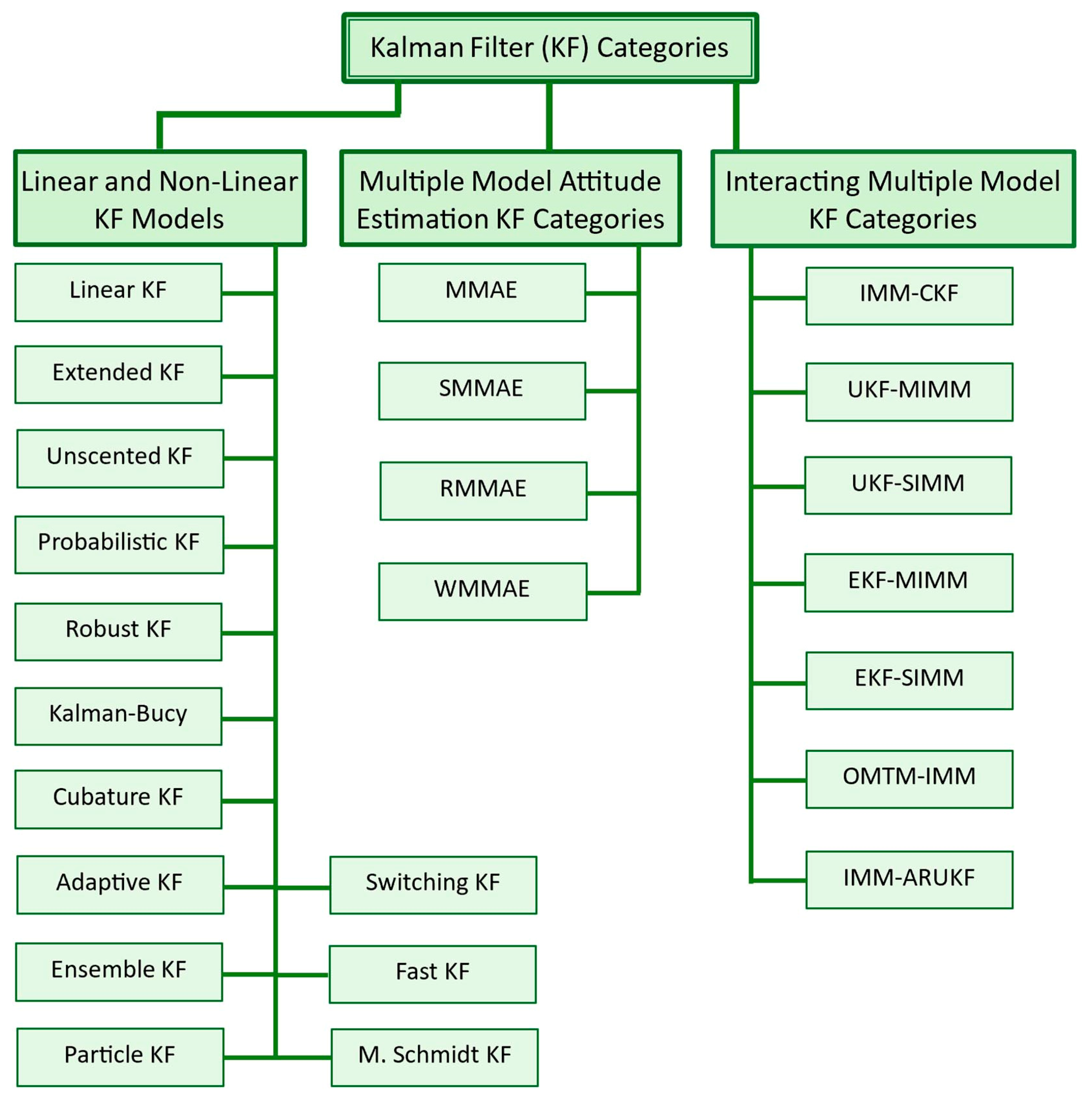
The diverse landscape of these filters is visually summarized in Figure 4. The diagram is organized to guide the reader from basic linear and non-linear observers in the left column, through the specialized MMAE configurations in the center, to the advanced IMM variants on the right. To facilitate further academic inquiry, all corresponding literature and foundational studies for each category are meticulously mapped within the figure [17,18,19,20,21,22,23,24,25,26,27,28,29,30,31,32,33,34,35,36,37,38,39,40,41,42,43,44,45,46,47,48,49,50].

Modeling complex system behavior is challenging, motivating the use of Multiple Model (MM) filters, where several filters representing different system models operate in parallel, and their outputs are combined for more reliable state estimation. Traditional MM filters struggle when system dynamics change, leading to the development of the Interacting Multiple Model (IMM) approach, which enables accurate transitions between models. Nevertheless, challenges such as parameter uncertainty, convergence issues, and high computational costs remain, driving ongoing research into improved model designs [51].

The MMAE algorithm is a widely used method for addressing model uncertainty. In MMAE, a set of discrete models approximates the uncertain system, with finer discretization requiring more models and thus higher computational cost [44,46]. MMAE has been successfully applied in applications including target tracking [52], error detection [53], and calibration bias correction [54]. Three generations of MMAE algorithms have been identified: the standard KF [55], the IMM [56], and the Variable-Structure Multiple Model (VSMM) [57]. While MMAE improves robustness to model uncertainty, poorly chosen or unstable model sets can still introduce residual errors.

To illustrate the adaptability of the KF framework, the following sections present three representative linear and non-linear filter models, highlighting their scalability and evolution over the decades.

A.

Extended Kalman Filter

The Extended Kalman Filter (EKF) serves as the primary non-linear extension of the traditional KF framework. Its core functionality revolves around the linearization of the system’s state space by approximating the mean and covariance through the current state estimates [17,18,19]. In an EKF setting, the state transition f and observation h models are expressed as non-linear, yet differentiable, functions of the state:

$$x_k=f(x_{k-1},u_{k-1}) w_{k-1}$$

(37)

$$z_k=h\left(x_k\right)+u_k$$

(38)

Here, $w_k$ and $u_k$ represent the process and observation noise vectors, assumed to be zero-mean multivariate Gaussian distributions with covariances $Q_k$ and $R_k$. Since non-linear functions cannot directly propagate uncertainties, the EKF calculates a Jacobian matrix—a matrix composed of partial derivatives—at each discrete time interval. These linearized matrices are then substituted into the standard KF update equations. This methodology has established EKF as the benchmark for navigation and GPS-based applications where transition models are analytically well-defined. Detailed applications of EKF within the realms of Electromagnetism, Quantum Physics, and Astrophysics are explored in subsequent chapters.

B.

Unscented Kalman Filter

In scenarios where system dynamics or observation models exhibit high degrees of non-linearity, the first-order linearization of the EKF often results in significant estimation errors or filter instability. The Unscented Kalman Filter (UKF) addresses these shortcomings by utilizing a deterministic sampling strategy known as the Unscented Transformation (UT) [20,21]. Instead of approximating the non-linear function, the UKF focuses on approximating the probability distribution. It selects a minimal set of sample points, termed sigma points, which are strategically positioned around the state mean. These points are then propagated directly through the actual non-linear equations, allowing for a more precise reconstruction of the posterior mean and covariance. This approach not only enhances accuracy for complex systems but also removes the computational and analytical burden of calculating Jacobians, which is particularly advantageous for non-differentiable models. The specific utility of UKF in High Energy Physics is detailed in the relevant section.

C.

Kalman–Bucy Filter

The Kalman–Bucy filter, named in honor of Richard Snowden Bucy, serves as the continuous-time analogue to the discrete-time KF [27,28]. This variant is built upon a continuous state-space representation that accounts for process and observation white noise:

$${\displaystyle \frac{d}{dt}}x\left(t\right)=F\left(t\right)x\left(t\right)+B\left(t\right)u\left(t\right)+w\left(t\right)$$

(39)

$$z\left(t\right)=H\left(t\right)x\left(t\right)+v\left(t\right)$$

(40)

In this context, $Q\left(t\right)$, Q(t) and $R\left(t\right)$, denote the power spectral densities of the white noise processes $w\left(t\right)$, w(t) and $v\left(t\right)$. Unlike the discrete KF, which strictly alternates between “predict” and “update” phases, the Kalman–Bucy filter operates through a continuous evolution described by two primary differential equations. The state estimate is governed by:

$${\displaystyle \frac{d}{dt}}\widehat{x}\left(t\right)=F\left(t\right)\widehat{x}\left(t\right)+B\left(t\right)u\left(t\right)+K\left(t\right)(z\left(t\right)-H\left(t\right)\widehat{x}\left(t\right))$$

(41)

while the error covariance $P\left(t\right)$ is determined by the following Riccati differential equation:

$${\displaystyle \frac{d}{dt}}P\left(t\right)=F\left(t\right)P\left(t\right)+P\left(t\right)F^T\left(t\right)+Q\left(t\right)-K\left(t\right)R\left(t\right)K^T\left(t\right)$$

(42)

The Kalman gain $K\left(t\right)$ is subsequently derived as:

$$K\left(t\right)=P\left(t\right)H^T\left(t\right)R^{-1}\left(t\right)$$

(43)

This filter is particularly significant in the study of electromagnetic fields, a topic further analyzed in the sections that follow.

4. Kalman Filtering in Thermodynamic Systems

Thermodynamic systems are inherently characterized by uncertainty, partial observability, and strong coupling between physical variables. Whether arising from modeling approximations, stochastic fluctuations at small scales, or noisy and incomplete measurements, these uncertainties fundamentally limit predictive accuracy and control performance. Within this context, Kalman filtering provides a unifying estimation framework that enables the systematic integration of physical models with observational data, allowing thermodynamic states to be inferred in a statistically optimal way.

This section reviews two distinct yet conceptually connected applications of Kalman filtering in thermodynamics. The first addresses large-scale thermo-fluid systems, where Kalman-based data assimilation is embedded into computational fluid dynamics solvers to mitigate model-form uncertainty and improve predictions of velocity and temperature fields. The second focuses on stochastic thermodynamic systems under continuous measurement and feedback, where the Kalman–Bucy filter emerges as the optimal estimator governing both information extraction and energetic performance. Despite their differences in scale and formulation, both approaches illustrate how Kalman filtering acts as a bridge between dynamics, uncertainty, and thermodynamic consistency.

4.1. Kalman-Based Data Assimilation in Thermo-Fluid Dynamics

A Kalman filter algorithm for computational thermo-fluid dynamics is proposed in [59] to improve thermodynamic systems evolution. As it is well known, in computational thermo-fluid dynamics (CFD), predictive accuracy is often constrained by the need to balance physical fidelity against computational cost [60]. Turbulence modelling, conjugate heat transfer, and complex boundary conditions introduce uncertainties that cannot be fully eliminated within practical Reynolds-Averaged Navier–Stokes (RANS) frameworks [61,62]. Kalman-based data assimilation offers a principled strategy, as shown in [59], to address these limitations by continuously correcting numerical solutions using experimental or real-time measurements.

Within this approach, the discretized conservation equations for momentum and energy are interpreted as a stochastic dynamic system. At each time step, the numerical solver provides a priori estimate of the velocity and temperature fields, along with an associated uncertainty. When observations become available, a Kalman update is performed, yielding a posteriori estimate that minimizes the estimation error in the Bayesian sense. This recursive structure aligns naturally with segregated finite-volume (FV) algorithms commonly employed in CFD, enabling the assimilation procedure to be incorporated without disrupting the solver’s architecture [63,64,65,66].

A particularly important feature of the methodology proposed in [59] is its explicit treatment of model uncertainty. Rather than assuming the numerical model is exact, uncertainties arising from turbulence closure, discretization, and unresolved physics are encoded through process noise, allowing measurements to systematically correct biased or incomplete predictions inherent so far in related calculations [67]. To preserve physical consistency, additional constraints are imposed to ensure mass conservation after each assimilation step, guaranteeing that the corrected velocity field remains divergence-free and compatible with the pressure and temperature solutions.

One of the most notable outcomes is the ability of the method to improve the estimation of both velocity and temperature fields even when only thermal measurements are available. Through the intrinsic coupling of the governing equations, corrections in the temperature field propagate to the momentum equations, leading to a globally improved flow prediction. From a computational standpoint, the added cost of Kalman-based assimilation remains moderate and is significantly lower than that required to achieve comparable accuracy through mesh refinement alone.

Overall, this application demonstrates how Kalman filtering can extend the practical limits of thermo-fluid simulations, transforming lower-fidelity CFD models into adaptive, measurement-informed predictors capable of robust performance in realistic heat transfer scenarios.

4.2. Kalman–Bucy Filtering, Information, and Thermodynamic Inequalities

In work [68], the traditional second law of thermodynamics is replaced by a family of second-law-like inequalities that explicitly incorporate information-theoretic quantities. Specifically, as established in [68], the traditional second law is generalized as ${\dot{S}}_{tot}\ge 0$, where the entropy production rate is expanded to include an information-theoretic term $\dot{I}$, leading to the relation ${\dot{S}}_{sys}+{\dot{S}}_{env}\ge -\dot{I}$. Here, $\dot{I}$ represents the information flow rate provided by the Kalman–Bucy filter, which is mathematically related to the reduction in the system’s uncertainty as captured by the filter’s covariance matrix. This formulation demonstrates that information acts as a thermodynamic resource, allowing for a consistent interpretation of entropy production and energetic balances in systems subject to continuous measurement and feedback. Within the broader context of stochastic thermodynamics, the Kalman–Bucy filter serves as a physical ‘benchmark’ that saturates the fundamental limits of information-to-energy conversion. This is possible because the Kalman approach provides advanced filtering capabilities and plays a fundamental role in stochastic thermodynamics, where systems are subject to continuous measurement and feedback. In such cases, thermodynamic evolution is no longer governed solely by energy exchanges but is intrinsically linked to information acquisition, processing, and control [69,70].

This perspective is illustrated through feedback cooling of a Brownian particle, a paradigmatic model for studying nonequilibrium thermodynamics with measurement and feedback [71]. In [68], the family of second-law-like inequalities incorporates information-theoretical quantities to quantify how measurement and feedback modify entropy production and energetic balances [72].

Recasting the feedback cooling problem within optimal control theory reveals that, under linear dynamics and Gaussian noise, the Kalman–Bucy filter provides the optimal estimate of the system’s state based on noisy observations. Importantly, this optimality is fundamental: no alternative estimation strategy can achieve a lower estimation error. The Kalman–Bucy filter thus represents the maximal achievable information extraction mechanism compatible with the system’s dynamics and noise statistics [73,74]. A key insight is that, when feedback control is based on the Kalman–Bucy estimate, distinct information measures—such as information flow and transfer entropy rate—coincide [75]. This equivalence arises because the Kalman–Bucy estimate constitutes a sufficient statistic, encapsulating all information relevant for predicting the system’s future evolution. As a result, the rate of information acquisition becomes uniquely defined and directly linked to thermodynamic quantities.

This convergence enables consistent thermodynamic interpretation of information: it establishes a unique lower bound on the energetic cost of measurement and feedback, clarifies the entropy production associated with information storage, and provides a rigorous definition of work extraction efficiency. In this framework, the Kalman–Bucy filter is not merely a mathematical tool but a thermodynamic benchmark that saturates fundamental bounds linking estimation, control, and energy.

The two applications reviewed in this section highlight complementary roles of Kalman filtering in thermodynamic systems. In large-scale thermo-fluid dynamics, Kalman-based data assimilation enhances predictive accuracy by systematically correcting model deficiencies using sparse measurements. In stochastic thermodynamics with feedback, the Kalman–Bucy filter defines the optimal mechanism for information extraction and reveals deep connections between estimation, entropy production, and energetic efficiency. Despite operating at different scales and addressing different physical questions, both approaches underscore a common principle: Kalman filtering provides a unifying framework for incorporating uncertainty and information into thermodynamic modelling. This perspective extends naturally to other classes of thermodynamic and energy systems, including reactive flows, phase-change processes, thermal management systems, and energy conversion devices. As will be shown in subsequent sections, Kalman-based methodologies continue to play a central role across a wide range of applications, offering both practical computational advantages and fundamental theoretical insights.

Overall, the synthesis of these applications reveals that Kalman filtering serves as a bridge between macroscopic data assimilation and microscopic stochastic thermodynamics. While Section 4.1 emphasizes practical predictive accuracy in fluid dynamics, Section 4.2 establishes the KF as a theoretical benchmark for information-to-energy conversion. Compared to traditional thermostatistics, the Kalman framework provides a dynamic advantage by explicitly accounting for the energetic cost of information acquisition.

5. Electromagnetism

The first work presented in this section proposes and assesses an inversion method based on Kalman Filters (KFs) and Extended Kalman Filters (EKFs) for the real-time detection and characterization of unexploded ordnance using electromagnetic induction dynamic data. A second study focuses on the estimation of electric and magnetic fields using the Kalman filter. The main idea centres on leveraging the Kalman filter’s capabilities as an optimal, real-time estimator to determine electromagnetic fields across an entire space, even when only sparse, discrete spatial measurements are available.

5.1. Real-Time Processing of Electromagnetic Induction Dynamic Data

The main idea of the work in [77] is to propose and validate an inversion method based on KFs and EKFs for the real-time detection and characterization of unexploded ordnance (UXO) using electromagnetic induction (EMI) dynamic data [78,79]. The conventional method for detecting UXO with EMI sensors involves two stages. In the first stage, large areas are surveyed in a dynamic mode to flag locations of interest based on the strength of the measured magnetic field while in the second stage sensors return to these flagged areas for more detailed examination [80,81]. A significant drawback of this amplitude-based flagging is that deeply buried UXOs might not produce a strong magnetic field response due to the rapid ${\displaystyle \frac{1}{R^6}}$ decay of the magnetic field with range, yet they can still pose a hazard.

To overcome this limitation, the authors in [77] introduce an iterative algorithm that combines KFs and EKFs. This method is designed to process dynamic data, in real time, acquired during rapid surveys and to provide estimates of both the UXO’s position and its polarizability (intrinsic features that aid in classification). KFs are stochastic signal processing techniques that use Bayes’ rule to estimate the state of a system from noisy measurements. While KFs are generally applied to estimate dynamic parameters, the work in [79] demonstrates their applicability in estimating stationary parameters like UXO position $\left(\overline{r^{\prime }}\right)$ and orientation $(\theta , \phi )$ [82], although the UXO itself is stationary. The algorithms work by recursively estimating a conditional probability density function in two steps: predict and update. In this specific application KFs are employed to estimate linear parameters, primarily the dipole moment $\left(\overline{m}\right(t\left)\right)$, from which the time-dependent polarizabilities can be derived. The dipole moment is considered a linear function of the magnetic field within the dipole approximation [83,84,85]. EKFs are used to estimate nonlinear parameters, specifically the UXO’s position $\left(\overline{r^{\prime }}\right)$ and orientation $(\theta , \phi )$. EKFs linearize the state and measurement equations to handle these nonlinearities.

The two types of filters (KF for polarizabilities, EKF for position and orientation) iteratively feed their estimates to each other until convergence is reached. Data are processed sequentially as they become available, whether by sweeping receiver positions, time channels, or transmitter positions. To enhance numerical stability, a Joseph-stabilized version of the EKF covariance matrix update equation is used. Additionally, a memory scheme is implemented to prevent solution divergence due to noisy dynamic measurements, retaining newly estimated parameters only if they result in a lower field mismatch.

The method in [79] was validated using two different EMI sensors, the Man Portable Vector (MPV-II) and the Metal Mapper, in various dynamic survey settings. The MPV-II was used in a handheld mode over a limited area with a single target, while the Metal Mapper was driven over long lanes containing multiple targets and clutter items. Despite the lower signal-to-noise ratio (SNR) characteristic of dynamic data collection, the KF-EKF algorithm consistently converged to accurate estimates, confirmed by comparison with a Gauss–Newton reference algorithm and ground truth data. Although the 2.7 ms data collection window in dynamic mode is typically insufficient for precise classification, the information provided by the KF-EKF algorithm, namely, position, depth, and limited polarizabilities, is often sufficient to identify a subsurface anomaly as a potential UXO. The dynamic data were processed by “G&G Sciences Inc.” using a technique based on a matched filter optimized for a spherical response, which enables a direct comparison of the results with our KF–EKF approach. This enables real-time target mapping and helps operators decide whether to proceed with more detailed cued interrogations at flagged locations. Finally, it should be noted that the paper points out the limitation that the algorithm assumes a Markov process of order 1 [86], meaning the current state depends only on the previous state. While this is a simplification for stationary targets where all past measurements could be used, it is a reasonable assumption for sensors like the Metal Mapper that continuously move across large areas.

While the first approach exploits Kalman-based inversion to estimate discrete object parameters from electromagnetic induction data, a complementary perspective is to treat the electromagnetic field itself as a dynamical state and reconstruct its spatio-temporal evolution directly from sparse measurements.

5.2. Stochastic Filtering in Electromagnetics

The authors in [87] focus on the estimation of electric and magnetic fields using the KF. The main idea is to leverage the KF’s capabilities as an optimal, real-time estimator to determine electromagnetic fields across an entire space, even when only sparse, discrete spatial measurements are available. The research presented in this paper introduces a method for estimating electric and magnetic fields throughout a given space. This estimation is crucial for various applications, including vehicle guidance, motion control, mobile communication base stations, medical diagnostic and therapeutic devices like transcranial magnetic stimulation (TMS), pedestrian dead reckoning, mine detection, power transmission fields, pipelines, and telecommunication lines [88,89,90].

The core of the proposed method in [87] involves the KF, which is a stochastic filtering technique. KF is used to estimate electric and magnetic fields by first estimating their underlying scalar and vector potentials. To apply the KF, the authors derive a state-space model based on the wave equations for these potentials, which include source terms (current and charge densities) and account for noise. Maxwell’s equations [91,92], which describe electromagnetic fields, are initially time-dependent first-order differential equations. They are reduced to two second-order wave equations for the scalar potential (Φ) and vector potential (A) [93]. These wave equations are then transformed into a finite-dimensional linear state variable model by discretising the spatial variables into pixels. The state vector includes the vector potential, its time derivative, the scalar potential, and its time derivative. To handle the discretised fields and partial differential operators efficiently, the Kronecker product is employed [94], allowing for a compact representation of the fields as vectors and operators as matrices. The electric and magnetic fields are expressed in terms of these potentials, and a measurement model is established. This model relates sparse discrete measurements of the electromagnetic field (e.g., from p pixels, where p is much less than the total number of discretised points $N^3$) to the state vector, including measurement noise.

The main advantage of the KF, which is a computationally efficient real-time algorithm, is its ability to directly account for both process noise (noise in the system dynamics, like in current and charge density) and measurement noise (noise in the observed field values). This makes it an optimal estimator that minimizes the mean square of the estimation error. This is crucial for applications requiring immediate field estimation. The proposed KF method is specifically implemented and tested on a Hertzian dipole antenna, a fundamental antenna element. The time-dependent current and volume charge densities of the dipole are used as source terms in the state-space equations. The KF algorithm involves an iterative process of initialization, time update (prediction of state and error covariance), and measurement update (calculation of Kalman gain and updating state and error covariance estimates).

The authors compare the KF with the Recursive Least Squares (RLS) method. While RLS is also a real-time algorithm, it primarily focuses on parameter estimation and uses only the measurement model, whereas KF considers the dynamics of the state and parameters, along with both process and measurement noise. The simulations demonstrate that the Kalman filter provides better estimation results than RLS, exhibiting lower Root Mean Square Error (RMSE) for both magnitude and phase estimation of electric and magnetic fields in both near-field and far-field scenarios. Ultimately, the paper highlights a significant contribution: the ability to estimate the entire (infinite-dimensional) electromagnetic field in space-time from only discrete spatial measurements, on a real-time basis. This is achieved by incorporating the a priori dynamics of Maxwell’s equations (even with noise) into the KF framework, opening new possibilities for field estimation, including in complex nonlinear media.

In the field of electromagnetics, the general lesson is that KF-based methods outperform traditional batch inversion (like Tikhonov regularization) in terms of real-time adaptability. Unlike batch methods that incur a heavy computational overhead by requiring full matrix inversions for each new data set, the recursive nature of the KF allows for efficient, sequential updates. The transition from induction data processing (Section 5.1) to broader stochastic filtering (Section 5.2) shows that while EKF is computationally efficient, its primary limitation remains the linearization error in highly non-linear EM fields, a challenge that is increasingly addressed by ensemble or unscented variations.

6. High Energy Physics

The article “Improving the Tracking of Subatomic Particles Using the Unscented Kalman Filter with Measurement Redundancy in High Energy Physics Experiments” presents an approach for improving particle tracking accuracy in high-energy physics (HEP) experiments, arguing that the UKF offers superior performance in handling non-linear dynamics and measurement uncertainties.

In a related study, the authors propose and evaluate a Non-Linear Kalman Filter (NLKF) for charged particle trajectory estimation, highlighting the limitations of the standard KF when its assumptions of linearity and Gaussian noise are violated in realistic tracking conditions.

6.1. Improving the Tracking of Subatomic Particles Using the Unscented Kalman Filter

The article [96] entitled “Improving the Tracking of Subatomic Particles Using the Unscented Kalman Filter with Measurement Redundancy in High Energy Physics Experiments” presents a method to enhance particle tracking accuracy in high-energy physics (HEP) experiments. The main idea of the article, focusing on the use of KFs, is that the UKF offers a superior solution for tracking subatomic particles in high-energy physics experiments [97] compared to the traditionally used EKF and non-linear filters like the CKF or Particle Filter (PF) [29,98,99,100,101], especially when dealing with high non-linearity and relative observability issues, and its performance can be further significantly improved by incorporating measurement redundancy.

The paper addresses the critical challenge of accurately determining the position and momentum of subatomic particles in HEP experiments where factors like multiple scattering and ionization energy loss complicate tracking [102]. These complexities lead to non-linear dynamics and relative (marginal) observability, causing the existing track reconstruction algorithm (EKF) to underperform or even diverge. The article proposes and investigates the UKF as an advanced alternative to the EKF.

While the EKF has been widely implemented in HEP experiments for particle trajectory reconstruction and detector alignment, it linearizes the non-linear system, leading to inaccuracies, particularly when dynamics are discontinuous. This linearization causes large errors in the posterior mean and covariance estimates, making the EKF suboptimal and prone to divergence due to factors like multiple scattering and weak observability from ionization energy loss. In contrast, the UKF avoids these linearization approximations. It employs a deterministic sampling approach, generating “sigma points” to capture the posterior mean and covariance more accurately (to the third order of a Taylor series expansion). This makes the UKF more robust to strong non-linearities originating from particles moving in strong magnetic fields and multiple scattering effects within detectors, as seen in the Muon Ionization Cooling Experiment (MICE) [103,104]. The UKF is also preferred over other non-linear filters like the CKF or PF because it balances accuracy with computational efficiency, which is crucial for processing the vast amounts of data generated by millions of particles in HEP experiments.

The paper specifically designs and analyzes the UKF for particle tracking in MICE, where an EKF is currently in use. It demonstrates that the UKF outperforms the EKF in terms of accuracy, achieving lower MSE in state estimates, especially under varying levels of non-linearity caused by process noise in strong magnetic fields. A significant contribution of the paper is the investigation into how measurement redundancy can further improve the UKF’s performance. Measurement redundancy is naturally incorporated into the UKF framework without requiring additional projection techniques.

The Kalman gain matrix contains more information, analogous to weighted averaging, when redundancy is introduced. The article examines two scenarios for introducing redundancy. The first one is duplicate measurements. This involves taking multiple measurements of the same quantity. Although often unrealistic in MICE due to hardware constraints, it generally leads to a significant reduction in MSE for the specific state being measured, especially if that state is affected by high noise. The second scenario is independent measurements. This more realistic approach involves using measurements of another variable, not necessarily part of the original state vector, as a redundant measurement. For example, the “Time of Flight” (TOF) of a particle, typically used for particle identification, is introduced as an independent redundant measurement. TOF significantly improves the estimates of longitudinal momentum (${\widehat{p}}_z$) and position ($z$) because it contains crucial information about the particle’s longitudinal path. Crucially, measurement redundancy is shown to improve the UKF’s performance from the perspective of relative observability and convergence.

Relative observability refers to the degree of accuracy with which a “weakly observable state” (a state estimated with significantly less accuracy than others) is determined relative to normal states. Ionization energy loss, for instance, can lead to weak observability, causing particles to drift or decay, thus providing inaccurate or no data. When a system becomes weakly observable, the condition number of the Fisher information matrix (FIM) (inverse of the error covariance) [105] or the updated covariance increases, potentially leading to filter divergence. By strategically introducing redundant measurements, especially those related to the weak state itself (duplicate measurements) or independent measurements that contribute information about it (like TOF for $p_z$ and $z$), the quality of these weak state estimates improves. In conclusion, this reduces the condition number of the covariance, enhances the system’s relative observability, and consequently improves the convergence and overall robustness of the UKF.

While the UKF with measurement redundancy significantly enhances robustness against non-linear dynamics and weak observability, further improvements can be achieved by explicitly reformulating the Kalman framework to handle strongly non-linear measurement models beyond linearization assumptions.

6.2. A Non-Linear Kalman Filter for Track Parameters Estimation in High Energy Physics

The researchers in [106] introduce, design and evaluate a NLKF to improve the estimation of charged particle trajectories (tracks) in high-energy physics experiments. The core idea of the article is that while the KF is a widely adopted and generally optimal algorithm for reconstructing charged particle trajectories in high-energy physics, its fundamental assumptions of linear dynamic systems and Gaussian noise distributions are often violated in real-world track reconstruction applications [107]. To overcome these limitations, the paper proposes and demonstrates an NLKF, which, unlike the commonly used EKF that linearizes the system, utilizes a set of representative sample points to directly account for non-linearities. This approach significantly improves the accuracy and precision of track parameter estimates, particularly in situations with high incidence angles where non-linear effects are pronounced, making it a promising solution for applications requiring high-precision track parameters.

The paper begins by establishing the KF as a cornerstone algorithm in nuclear and particle physics for the reconstruction of charged particle trajectories, also known as tracks. The KF, processes discrete measurements to determine the internal state of a dynamical system, minimizing the impact of random perturbations (noise). It is used both in track finding (identifying measurements belonging to a single particle) and track fitting (determining trajectory parameters) [108,109].

Typically, KF algorithms start with a “track seed” and progressively add measurements, followed by a smoothing operation. However, a significant limitation of the standard KF, and even its extension, the EKF, lies in their assumptions of linear models for the system and measurements, and Gaussian distributions for process and measurement noise. These assumptions are frequently violated in high-energy physics due to complex factors like inhomogeneous magnetic fields, detector material interactions, and non-linear dependencies of measurement positions on track direction. While the EKF attempts to linearize the system using a first-order Taylor expansion, it proves insufficient when particles hit detector surfaces at large incidence angles. Other extensions like the Gaussian Sum Filter (GSF) address non-Gaussian process noise (e.g., radiative energy loss for electrons) but do not tackle non-linear measurement models) [110].

To address these non-linear challenges, the authors of the paper introduce an implementation of a NLKF within the ACTS track reconstruction toolkit. This NLKF is based on the UKF, which handles non-linearity by using a set of “sample points” to parameterize the mean and covariance during the projection of the track state to the measurement, rather than relying on linearization. The NLKF considers 2N + 1 sample points around the mean of the track state, where N is the dimension of the track state vector (e.g., 8 for global track parameters), with each point assigned a weight. These sample points are propagated and projected through the non-linear track and measurement models and then used to calculate the mean and covariance of the projected state. The performance of the NLKF was evaluated using a simulated Open Data Detector (ODD) [111].

The results show that the NLKF consistently outperforms the EKF in terms of accuracy and precision. Specifically, The NLKF eliminates biases in the mean of residuals for perigee track parameters observed with the EKF, especially at higher pseudo rapidity $\left(\right|\eta \left|\right)$ regions where non-linear effects are significant. Additionally, it improves the resolution of impact parameters by up to 80% in high $\left|\eta \right|$ bins compared to the EKF. Furthermore, the Root-Mean-Square (RMS) of the pull distributions for track parameters (which ideally should be one) is significantly closer to one across a wider range of $\left|\eta \right|$ when using the NLKF, indicating a more accurate estimation of parameter uncertainties. This improvement is particularly pronounced for tracks with larger transverse momentum ($pT$). While the NLKF does incur an increased computational cost, with track fitting time rising by a factor of approximately 1.6 to 1.8 compared to the EKF, this increase is considered negligible for overall track reconstruction time in most applications, as track fitting is typically not the most time-consuming step.

In conclusion, the article demonstrates that the NLKF is a promising approach for charged particle track reconstruction in high-energy physics.

Synthesizing the developments in high-energy physics, it is evident that the shift from standard KF to non-linear variants like UKF is driven by the extreme precision required in subatomic particle tracking. Unlike classic least-squares fitting, the recursive nature of the UKF allows for the integration of non-Gaussian noise and complex trajectory constraints, making it the superior choice for modern collider data reconstruction where computational speed and track resolution are equally critical.

7. Quantum Physics

The application of the KF in measurements regarding quantum physics and physical phenomena laying at the atomic scale is discussed in this section by means of two representative manuscripts. The first concerns the application of the KF in Atomic Magnetometry so that the Heisenberg limit is achieved as far as the reduction in the shot-noise is concerned. The other one regards the introduction and formulation of a quantum EKF, which is designed to efficiently estimate the state of nonlinear open quantum systems subject to noisy measurements.

We must briefly elucidate the essential differences between quantum systems and classical systems in filtering problems at a high level. Specifically, in classical filtering the system evolves independently of observation while in quantum filtering, we must account for the fact that observing the system alters its future evolution. Classical filtering is governed by deterministic or stochastic differential equations however quantum filtering is governed by operator equations. In classical filtering standard probability theory applies whereas in quantum filtering you cannot simultaneously estimate all quantities precisely while the order of measurements matters. Theoretically, in classical filtering we estimate a hidden variable from noisy data on the contrary in quantum filtering, we estimate a state that is both uncertain and is altered by the act of estimation itself.

7.1. Quantum Kalman Filtering and the Heisenberg Limit in Atomic Magnetometry

The central theme of article [112] is the development of an optimal parameter-estimation method in atomic magnetometry that surpasses the traditional shot-noise limit of ${\displaystyle \frac{1}{\sqrt{N}}}.$ This is achieved by integrating continuous quantum measurements with a Quantum Kalman Filter (QKF). This approach achieves the enhanced ${\displaystyle \frac{1}{N}}$ field sensitivity characteristic of the Heisenberg limit [113]. A key challenge in reaching sub-shot-noise performance is to take advantage of conditional spin squeezing, which naturally arises through the continuous monitoring of an atomic ensemble [114]. The QKF provides the optimal strategy for extracting information from this squeezed state.

Magnetometry is presented as a fundamental parameter estimation process where the strength of a magnetic field must be derived from its effect on a detector such as an atomic spin ensemble. In high-precision magnetometers the detection limit is determined by the shot noise, which has a limit determined by the occurrence of quantum fluctuations for a set of N atoms and scales to ${\displaystyle \frac{1}{\sqrt{{\rm N}}}}$. This limit is derived from the projection noise, which is equal to ${\displaystyle \frac{J}{2}}$ when measuring ${\widehat{J}}_z$ for a spin state ($〈{\widehat{J}}_t〉$ is the Bloch vector).

The procedure followed in this work combines continuous measurement and quantum Kalman filtering to overcome this conventional limit and achieve a ${\displaystyle \frac{1}{{\rm N}}}$ field sensitivity that is characteristic of the Heisenberg limit. To do this, it exploits the creation of conditional spin squeezing that is automatically generated by the observation of the atomic sample. It should be noted here that the ${\displaystyle \frac{1}{{\rm N}}}$ field sensitivity is the reference limit that signals the achievement of the Heisenberg limit, which represents the maximum possible sensitivity that can be achieved when measuring a physical quantity such as the magnetic field when a set of N atoms is used.

Accordingly, this is achieved by

• Developing the spin compression process called spin squeezing.
• Continuous measurement and filtering with a QKF.

The QKF allows high bandwidth magnetometry to reach the Heisenberg limit and the linear regression method achieves ${\displaystyle \frac{1}{J}}$ (or ${\displaystyle \frac{1}{N}}$) scaling for long times. On the other hand, spin squeezing decreases the projection noise of the measured spin component ${\widehat{J}}_z$ below the standard quantum limit [115]. However, the process of continuous observation generates a stochastic transient that can localize the conditional expectation value ${〈 {\widehat{J}}_z〉}_c$ around a random offset. This produces noise in the measured photocurrent even when no magnetic field is applied making it difficult to separate true Larmor precession from measurement-induced fluctuations. The QKF resolves this problem. Built from quantum trajectory theory [116], the QKF provides the optimal estimate of the magnetic field by correctly interpreting the continuously evolving conditional spin state. In doing so, it utilizes the spin squeezing [117] while avoiding confusion between genuine Larmor precession and stochastic Bloch-vector fluctuations. As a result, the method enables Heisenberg-limited magnetometric precision despite the presence of optical shot noise and transient measurement effects. For fixed atom number (N) and measurement time (t), the QKF delivers greater precision than standard steady state magnetometry.

The implementation relies on a recursive estimation procedure that incorporates the probabilistic nature of quantum measurements and consists of the following steps:

a. Modelling Conditional Quantum Dynamics

The atomic sample undergoes a continuous quantum nondemolition (QND) measurement of ${\widehat{J}}_z$. Its conditional density operator ${\widehat{\rho }}_c$ evolves according to a stochastic master equation containing three elements:

The first one is a Hamiltonian term producing the Larmor precession that encodes the magnetic field (B), the second one is a measurement-induced decoherence, which reduces the Bloch vector length, and the last one is a stochastic term representing optical shot noise. Under a Gaussian approximation, only the mean ${〈{\widehat{J}}_z〉}_c$ and variance $〈\Delta {\widehat{J}}_z^2〉$ are needed to describe the atomic state. Their dynamics capture deterministic precession, stochastic diffusion, and the reduction in variance associated with conditional squeezing.

b. Determining the Optimal Estimator

The aim is to evaluate the conditional probability distribution $p\left(B\right|I_{0,t})$, the likelihood of a field value (B) given the measurement record $I$. Updating this distribution optimally requires Bayesian inference, applied iteratively as measurement data accumulate.

c. Applying the Recursive Quantum Kalman Filter (RQKF)

This iterative Bayesian update is efficiently carried out through a recursive KF. The QKF tracks the state vector $\tilde{x}={({\tilde{J}}_z,\tilde{B})}^T$, where ${\tilde{J}}_z$ is the estimated conditional spin component and $\tilde{B}$ is the estimated magnetic field. The estimation accuracy is described by a covariance matrix $V\left(t\right)$, which evolves according to a matrix Riccati equation. Spin squeezing and Bloch vector decay influence this evolution, ultimately yielding optimal estimates of both the field $\tilde{B}$ and its uncertainty.

d. Relation to Linear Regression

For static (time-independent) magnetic fields, the optimal QKF strategy can be closely approximated by simple linear regression. While the QKF performs better at short times, the two approaches converge once the measurement duration exceeds roughly $t\ge {\left(JM\right)}^{-1}$. At this stage, the regression fit absorbs the initial stochastic transient into its intercept, and both methods achieve the Heisenberg-scaling ${\displaystyle \frac{1}{J}}$ (or ${\displaystyle \frac{1}{N}}$) precision. This observation suggests that linear regression may offer a practical and experimentally simple pathway to sub-shot-noise sensitivity.

While the QKF enables Heisenberg-limited performance in a specific sensing application under effectively linearized quantum dynamics, more general quantum systems exhibit intrinsic nonlinearities that require extensions beyond the standard Kalman filtering framework.

7.2. A Quantum Extended Kalman Filter

The main idea of article [118] is the introduction and formulation of a quantum extended Kalman filter (quantum EKF), which is designed to efficiently estimate the state of nonlinear open quantum systems subject to noisy measurements. This filter is presented as a computationally efficient recursive alternative to methods presented in the past for quantum filtering [119,120,121]. The ability to effectively measure and control complex quantum systems requires a method, known as filtering in control engineering, to infer the expectations and variances of unknown observables from noisy measurements using a dynamic model.

In quantum physics, the optimal filter in the Schrödinger picture is commonly known as the stochastic master equation (SME) [122,123], which estimates the state (density operator) of a quantum system. However, the real-time application of the SME for general quantum systems is computationally difficult because the computation time scales exponentially with the size of the Hilbert space basis, making it hard to implement in real-time.

The Role of the Classical KF is to be a computationally efficient recursive dynamic state estimator. When classical dynamics are linear and noise covariances are known, the KF is the optimal linear filter [124]. The EKF generalizes the KF to handle nonlinear systems by using linearization (specifically, first-order Taylor approximations), maintaining computational efficiency, even though it is no longer an optimal filter [125,126,127].

For quantum systems where the dynamics are described by linear quantum stochastic differential equations (QSDEs) subject to linear measurements and Gaussian noise, the quantum filter already simplifies to a QKF. The central contribution of this article is the development of the quantum EKF, which adapts the EKF structure for systems governed by nonlinear QSDEs. This adaptation involves applying a commutative approximation and a time-varying linearization. The main challenge in quantum filtering is that the system’s observables generally consist of non-commuting operators. The implementation of the quantum EKF relies on the assumption that the estimated state belongs to a commutative von Neumann algebra [128]. This property is crucial because it allows the filter dynamics to be transformed into a standard ordinary stochastic differential equation (SDE), like the classical EKF. This transformation enables the quantum EKF to be implemented as a recursive filter in a digital signal processor.

By leveraging the computational structure of the EKF, the quantum EKF achieves immense efficiency gains compared to the SME. For example, in estimating the quadrature of two cavity modes, the SME required nearly 200 times the computational time of the quantum EKF. This ratio increases dramatically up to 170,000 times if the number of modes is increased to three. The article establishes a sufficient condition under which the quantum EKF maintains local quadratic exponential convergence in the estimation error, guaranteeing boundedness. Furthermore, the authors introduced a modification, the robust quantum EKF (rqEKF), to handle cases common in quantum systems, such as when variance matrices for process and measurement noises are state-dependent (functions of the system observables). In the final analysis, the effectiveness of the quantum EKF is demonstrated through applications, including the estimation of quadrature in multiple cavity modes with Kerr nonlinearities, and systems subject to simultaneous homodyne detection and photon counting measurements (which involve state-dependent covariances) [129].

A cross-study analysis in quantum physics highlights that the QKF is not merely an estimation tool but a necessity for reaching the Heisenberg limit. The studies reviewed indicate that while the Extended QKF handles the inherent non-linearity of quantum measurements, the fundamental strength of the Kalman approach lies in its ability to maintain optimal state estimation under continuous weak measurements, providing a more robust framework than traditional project-based quantum state tomography.

8. Astrophysics

An important application of the KF in astrophysics is reviewed in this section, which focuses on the development and application of Kalman filter-based control techniques to optimize fringe tracking in optical interferometers. Furthermore, elementary particle tracking using the KF approach is the main idea of the second method described, which presents approaches based on the KF for the critical task of track reconstruction in high-energy underwater Cherenkov neutrino telescopes.

Together, these two applications illustrate how Kalman filtering enables optimal state estimation in astrophysical systems characterized by sparse observations, strong noise, and stringent real-time constraints.

8.1. Kalman Filter-Based Control Techniques to Optimize Fringe Tracking in Optical Interferometers

An important application of the KF in astrophysics is the one presented in article [131], which focuses on the development and application of Kalman filter-based control techniques to optimize fringe tracking in optical interferometers. This methodology is specifically designed for GRAVITY [132], a future four-telescope near-infrared beam combiner intended for the Very Large Telescope Interferometer (VLTI). Implementing fringe tracking in optical interferometers becomes essential when aiming to fully optimize the instrument’s performance. By enabling continuous fringe monitoring, fringe tracking greatly enhances the sensitivity of the interferometric setup. Beyond compensating for atmospheric path-length variations, an effective control system must also correct disturbances caused by mechanical vibrations within the instrument and handle additional errors that arise along the optical paths. In this context, fringe tracking can be naturally formulated as a state estimation and control problem, making Kalman filtering particularly well suited for this application.

The main idea is that constructing control schemes based on KFs allows for an improvement upon existing fringe-tracking control [133], particularly in dealing with instrumental vibrations [134], and provides the capability to maximize tracking performance. The KF is used to track and correct observed systems in a statistically optimal way, meaning it minimizes the norm of the residual signal for linear systems operating under Gaussian noise statistics. In many physical problems, including this one, the experimental setup inherently contains certain sources that introduce errors into the measurements. Since the problem is parametric, parameter identification is required. By using the KF algorithm, these errors can be reduced or even eliminated by combining the actual experimental measurements with the optimal estimation provided by the filter. In this way, the obtained result is based both on the experimental data and on the optimization of the error factors that arise in the measurements.

A crucial requirement for using the KF is an a priori model that describes the perturbations of fringe phases, such as turbulence and vibrations. This model allows the filter to optimize tracking based on the prevailing disturbances. The perturbations are described by the evolution of the observed system, which is cast into a time-invariant state-space representation consisting of a recursive equation of state and an observation equation [135]. First, the KF estimates the system’s hidden state vector from the observations. The filter updates the estimate of the disturbance state based on the current measurement and then predicts the state at the subsequent moment. After that, the matrix known as the Kalman gain determines the weight given to the new measurement when updating the state estimate. The last step is that the optimal command sent to the Optical Path Difference correcting actuators is calculated based on the predicted next state to minimize the residual optical path difference [136].

The use of Kalman filtering offers several advantages over classical control strategies (e.g., integrator control) in the context of fringe tracking. It is a statistically optimal control method because it incorporates all information on disturbances means of the a priori model. Another advantage is that it allows turbulence and longitudinal vibrations to be controlled coherently and equivalently and that also decomposes the contribution of different perturbation components. Finally, an important parameter is that it has a predictive nature, which allows the control scheme to deal with the loss of observables, such as short-time signal absence due to flux problems (flux dropouts). Moreover, the study extended the basic two-telescope KF scheme to handle four-telescope interferometry, which measures six Optical Path Differences but uses only four actuators. To ensure robustness against issues like low signal-to-noise baselines and flux dropouts, both schemes include mechanisms to adapt to variable observation quality.

The effectiveness of the Kalman-filter-based control strategy is ultimately assessed through end-to-end simulations under realistic disturbance and noise conditions. The simulations for GRAVITY aiming for a residual Optical Path Difference specification of 300 nm, demonstrated that the KF scheme provided the best results for the Optical Path Difference. This scheme achieved an average residual rms Optical Path Difference of about 240 nm. On the other hand, the modal scheme performed slightly worse (average of 290 nm), possibly because all vibration parameters must be extracted simultaneously during identification, which is more difficult than fitting individual Optical Path Difference periodograms, but ultimately, it turns out that both schemes showed performance compatible with the 300 nm stability required for GRAVITY’s principal science case. The simulations also indicated that the KF control schemes are rather unaffected by the considered flux perturbations, as there was no significant difference in performance between fixed and instantaneous gains for the sequences tested. Evidently, the KF based control schemes are likely to become the next standard for fringe tracking. The results of this study are being incorporated into the final design of GRAVITY.

While the previous application focuses on Kalman filtering as a predictive control tool for optical interferometry, the following subsection examines its role as a sequential reconstruction and filtering framework in high-energy neutrino astronomy.

8.2. A Kalman Filter Approach for Track Reconstruction in a Neutrino Telescope

Elementary particle tracking using the KF approach is the main idea of article [137]. In this case, Kalman filtering is employed not only as a fitting tool, but as a probabilistic framework for disentangling signal from background in a highly noisy measurement environment. This work presents methods based on the KF approach for the critical task of track reconstruction in high-energy underwater Cherenkov neutrino telescopes [138]. The track reconstruction process in neutrino telescopes is complex because the environment introduces significant measurement noise and non-linearities. Neutrino telescopes detect neutrinos indirectly through Cherenkov light produced by secondary leptons (muons). However, several factors complicate the accurate measurement of the muon track, such as, electromagnetic showers accompanying high-energy muons generate Cherenkov light [139,140], photon scattering in the water introduces non-Gaussian measurement noise and environmental background, primarily the isotropic background of photons resulting from the beta-decay of the potassium isotope causes a large noise counting rate. These factors lead to a non-linear problem with non-Gaussian measurement noise that must be resolved for accurate track identification.

The KF is utilized as an efficient algorithm for track filtering and fitting that is particularly adapted to sequential measurements. The KF approach treats the track as a dynamic system described by a state vector $x$, working through a two-step recursive process. The prediction step, which estimates the true unknown values and the measurement step, where once the measurement outcome is observed, these estimates are updated using a weighted average. The KF allows for the track parameters to be progressively evaluated, improving knowledge of the track iteratively with each measurement. Furthermore, the KF technique is effective at rejecting uncorrelated noise signals, such as the optical background from $\beta$-decay of potassium isotope ${}^{40}K$, by associating a probability to each hit belonging to a track. Because of its recursive nature, the filter can potentially run in real time.

In high energy neutrino telescopes, the detection principle relies on the detection of Cherenkov light emitted from an up-going muon induced by nm that have penetrated the Earth. In the muon energy range of interest for astro physical searches (namely, from about 100 GeV to about 1 PeV), the electromagnetic showers accompanying the muon track generate Cherenkov light emitted within a few degrees of the cone associated with the primary particle. Furthermore, because of photon scattering in the water, the measurement is affected by non-Gaussian noise. Consequently, track reconstruction in underwater Cherenkov neutrino telescopes is strongly complicated. Moreover, environmental background originates large noise counting rates. In an undersea neutrino detector, in fact, the decay of radioactive elements, mainly the b-decay of potassium isotope 40K, generates electrons that produce Cherenkov light leading anisotropic background of photons. Therefore, the hit pattern identification of neutrino induced event is non-trivial and the track reconstruction has to deal with a non-linear problem due to this non-Gaussian measurement noise. This motivates the use of advanced Kalman-based strategies capable of handling non-linearity and non-Gaussian noise beyond the assumptions of the standard KF. In the paper under examination, a method based on the Gaussian Sum Filter algorithm to consider non-Gaussian process noise for track reconstruction in a km3 underwater neutrino telescope is presented. To specifically address the difficulty of the non-Gaussian measurement noise [141], article [137] proposes and studies two sophisticated methods based on the KF strategy:

The first method utilizes the EKF approach, which is suitable for the non-linear relationship between track parameters and the measurement (hit-time) in neutrino telescopes. The EKF recognizes that photons that have scattered or originated from secondary electrons are often delayed compared to the prompt photons that carry the most precise timing information. To account for these delays, the residual distribution is approximated using a Gaussian distribution, but its mean is shifted to an appropriate value ($r>0$).

The other method is the Gaussian Sum Filter [110]. In this case, more accurately accounts for the non-Gaussian distributions of measurement errors. The measurement error distribution is approximated by a sum of several Gaussian distributions (a Gaussian mixture), where the core corresponds to the principal component and the tails are modelled by additional Gaussians. The Gaussian Sum Filter effectively resembles a set of KFs running in parallel, with each filter corresponding to one component of the state vector mixture. While a strict application of the Gaussian Sum Filter leads to a prohibitively large number of components, a re-sampling algorithm is used to reduce the components, keeping about 50 for good performance.

Both the KF and the Gaussian Sum Filter approaches are based on the KF Strategy. Comparisons of the performance of the methods show that the Gaussian Sum Filter provided superior results in estimating track coordinate and angle parameters compared to the KF Strategy method, as shown by lower median values and Gaussian sigma for angular and coordinate residuals. In

Table 1. Performance Comparison of Gaussian Sum Filter and Kalman Filter Strategy. $m_{\theta }$ is the median of the distribution of space angle deviation between the reconstructed and the simulated muon track (mrad), ${\sigma }_{\theta }$ is the Gaussian sigma for parameter $\theta$ residuals (mrad), and ${\sigma }_X$ is the Gaussian sigma for X-coordinate parameter residuals (m).

Method	${\mathit{m}}_{\mathit{\theta }}$	${\mathit{\sigma }}_{\mathit{\theta }}$	${\mathit{\sigma }}_{\mathit{X}}$
Gaussian Sum Filter	2.00	0.96	0.53
Kalman Filter Strategy	12.3	6.90	4.08

(according to [68]) the comparison of the performances of the Gaussian Sum Filter method and the KF.

In astrophysics, the common thread between optical interferometry and neutrino detection is the management of extremely low signal-to-noise ratios. The synthesis of these applications suggests that the KF’s ability to provide real-time optimal control (fringe tracking) and efficient track reconstruction (neutrino telescopes) offers a significant advantage over static filtering. The KF framework proves indispensable for handling the sparse and noisy data streams typical of deep-space observation.

9. Conclusions

The KF has long been regarded as the optimal solution to the analysis of many tracking, data prediction and physical problems. The filter is constructed as a mean squared error minimizer, but an alternative derivation of the filter is related to maximum likelihood statistics. How well a filter performs this task can be measured using a cost or loss function, the minimization of which defines the goal of the filter. In this work, before reviewing the KF applications in Physics, we explained the KF algorithm analytically. After that, we elaborated on the categories of KF and explained the operation of each one, as well as 10 special example cases for better understanding KF application in Physics were presented. However, the KF has several advantages; it bypasses the need to determine the impulse response of the filter, something that is poorly suited to numerical computation. Kalman described his filter using state space techniques, which enables the filter to be used as either a smoother, a filter or a predictor. For the latter of these three, the ability of the KF to be used to predict data has been applied to a wide range of tracking, visual motion tasks and navigation problems, some of which were presented in this work.

The purpose of filtering is to extract the required information from a signal, ignoring everything else. How well a filter performs this task can be measured using a cost or loss function. Indeed, we may define the goal of the filter to be the minimization of this loss function.

The present work has investigated Kalman filtering as a unifying framework for state estimation across a broad spectrum of physical systems characterized by uncertainty, partial observability, and noisy measurements. By surveying applications ranging from thermodynamic and electromagnetic systems to high-energy, quantum, and astrophysical contexts, we have highlighted how Kalman-based methodologies surpass their original role as estimation algorithms and instead function as principled mechanisms for integrating physical models with information extracted from data.

This review demonstrates that the KF serves as a profound unifying framework that bridges physical modeling, uncertainty quantification, and real-time information processing across highly diverse domains. By comparing its applications from thermodynamics to astrophysics, a key insight emerges: the filter’s success in physics does not stem merely from its algorithmic efficiency, but from its unique ability to enforce physical consistency (such as conservation laws or thermodynamic constraints) within a stochastic estimation loop. When developing these filters for physical and mechanical systems, a critical trade-off arises between the EKF and the UKF. EKF is based on first-order linearization, making it computationally frugal and ideal for high-dimensional systems or real-time applications with limited processing power. However, it is prone to drift in strongly nonlinear environments. In contrast, UKF captures higher-order nonlinearities using a deterministic set of sigma points without requiring complex Jacobian calculations. This gives the UKF superior robustness and higher accuracy (critical for quantum or high-energy physics applications), albeit at a higher computational cost. Therefore, EKF is preferable for mild nonlinearities and time-critical loops, while UKF is chosen when the accuracy and stability of the filter outweigh the processing time.

A central insight emerging from this review is that the effectiveness of Kalman filtering in physics is not solely determined by algorithmic sophistication, but by the alignment between the filter structure and the underlying physical assumptions. Across all domains considered, successful implementations explicitly encode system dynamics, noise statistics, and measurement constraints in a manner consistent with physical laws and experimental realities. In this sense, Kalman filtering serves not only as a tool for estimation, but also as a lens through which model inadequacies, dominant uncertainty sources, and information bottlenecks can be systematically identified and addressed.

Moreover, the presented fields of Physics are given in the appropriate order since they can be seen to be related if we treat the KF as a universal tool for estimating hidden states from noisy measurements. Consequently, in Thermodynamics, the KF infers evolving macroscopic states (e.g., temperature fields) from sparse/noisy sensors. Here uncertainty arises from many-body averaging. In Electromagnetism, the system becomes more structured, and fields obey deterministic equations (Maxwell’s equations) while noise now comes from sensors, environment, or modeling errors. In High-energy physics, we track particles through detectors. Here, KFs reconstruct particle trajectories (e.g., in colliders), so we shift from continuous fields to discrete, probabilistic event reconstruction. In Quantum physics, uncertainty is no longer just practical, but it is fundamental (Heisenberg uncertainty principle). Classical KFs are extended into “quantum filters” (e.g., stochastic Schrödinger equations). Noise is not just measurement error; it is intrinsic to reality. Finally, in Astrophysics, we may combine all previous elements. All uncertainties combine across scales and physical laws.

The reviewed applications further demonstrate that Kalman-based approaches are particularly powerful in regimes where uncertainty is intrinsic rather than incidental. In thermo-fluid and stochastic thermodynamic systems, filtering frameworks reveal deep connections between estimation, irreversibility, and information flows. In electromagnetic and astrophysical applications, they enable spatially and temporally extended inference from sparse data, effectively compensating for limited sensor access. In high-energy and quantum-scale systems, advanced Kalman variants merge nonlinear dynamics and measurement back-action with real-time state reconstruction, underscoring the adaptability of the framework across physical scales.

Looking forward, several promising research directions emerge. First, the integration of Kalman filtering with data-driven and machine-learning-based models offers a pathway toward hybrid estimation frameworks that combine physical interpretability with enhanced representational power. Such approaches may be particularly impactful for complex systems where first-principles models are incomplete or computationally prohibitive. Second, the extension of Kalman-based methods to strongly nonlinear, non-Gaussian, and non-Markovian schemes remains an open challenge with significant relevance for turbulence, quantum many-body systems, and nonequilibrium statistical physics. Third, increasing experimental demands for real-time inference and control call for scalable, adaptive filtering strategies capable of operating under stringent computational and latency constraints.

More broadly, the continued relevance of Kalman filtering in modern physics reflects its foundational role at the intersection of dynamics, uncertainty quantification, and information theory. As experimental systems become more complex and data-rich, yet remain fundamentally constrained by noise and partial observability, Kalman-based methodologies are poised to remain essential components of the physicist’s inference toolkit. Future developments that further tighten the coupling between estimation theory and physical modeling are likely to not only improve predictive performance but also deepen our understanding of how information is acquired, processed, and utilized in physical systems.