Integrating SVR Optimization and Machine Learning-Based Feature Importance for TBM Penetration Rate Prediction

Abstract

In this study, a Support Vector Regression (SVR) model was developed to predict the rate of penetration (ROP) during tunnel excavation, and its hyperparameters were optimized using Grid Search (GS), Random Search (RS), and Bayesian Optimization (BO). The results indicate that BO reached the optimal parameter set with only 30–50 evaluations, whereas GS and RS required approximately 1000 evaluations. In addition, BO achieved the highest predictive accuracy (R² = 0.9625) while reducing the computational time from 25.83 s (GS) to 17.31 s. Compared with the baseline SVM model, the optimized SVR demonstrated high accuracy (R² = 0.9610–0.9625), strong stability (NSE = 0.9194–0.9231), and low error levels (MAE = 0.0927–0.1099), clearly highlighting the critical role of hyperparameter optimization in improving model performance. To enhance interpretability, a feature importance analysis was conducted using four machine learning methods: Random Forest (RF), Bagged Trees (BT), Support Vector Machines (SVM), and the Generalized Additive Model (GAM). The relative contributions of BI, UCS, ALPHA, and DPW to ROP were evaluated, providing clearer insight into the model’s decision-making process and enabling more reliable engineering interpretation. Overall, integrating hyperparameter optimization with feature importance analysis significantly improves both predictive performance and model explainability. The proposed approach offers a robust, generalizable, and scientifically sound framework for TBM operations and geotechnical modeling applications.

1. Introduction

Modern transportation, energy, and infrastructure projects rely on tunnels to ensure the continuity of intercity and regional transportation, as well as to support water supply, wastewater management, and energy transmission. Tunnel Boring Machine (TBM) modeling is a critical engineering discipline that enables the practical implementation of governmental directives on infrastructure planning, urban development, environmental protection, and resource management. The realization of safe, economical, rapid, and environmentally efficient tunnel projects demanded by public authorities depends on the scientific modeling of TBM performance, early prediction of risks, and the optimization of energy and material use. In this context, TBM modeling aligns with sustainable development goals and governmental policies such as low-carbon infrastructure and urban resilience by making tunneling processes more efficient, environmentally safer, and technically more predictable.

Optimizing energy consumption, cutter wear, and project duration reduces resource use while lowering the carbon footprint; accurate prediction of ground behavior helps mitigate environmental risks such as surface settlements and groundwater impacts. All these improvements directly contribute to the development of sustainable, resilient, and environmentally compatible infrastructure by reducing costs, enhancing occupational safety, and minimizing adverse social impacts.

However, since tunneling operations are performed under complex geotechnical conditions and variable ground properties, significant costs, safety risks, and technical challenges emerge during the design, construction, and operation phases. Therefore, the efficient and safe excavation of tunnels depends directly on the accurate prediction of Tunnel Boring Machine (TBM) performance. Reliable estimation of the TBM rate of penetration (ROP) is of critical importance for planning excavation operations and controlling project costs.

Early research on TBM penetration rate prediction [1] began with empirical models based on rock strength, followed by studies focusing on TBM performance in sedimentary environments [2]. The first statistical regression model establishing the relationship between rock properties (UCS, PSI, DPW, α) and penetration rate was proposed by [3]. The brittleness index (BI), the mean distance between weak planes (DPW), and the angle between the tunnel axis and weak planes (α) are among the most significant variables influencing TBM performance. When evaluated together with other factors, these three parameters enable a holistic modeling of sustainable penetration capacity by accounting for the applied cutting load and cutter wear.

Thanks to advanced regression analysis, this model achieved a high correlation (r = 0.82) and provided an empirical estimation equation based on measured rock parameters [3]. However, these early approaches were mostly limited to simple correlations and were insufficient for capturing complex geotechnical interactions.

Heuristic optimization algorithms were first applied to TBM performance prediction by Yağiz and Karahan [4], who developed a particle swarm optimization (PSO)-based model aimed at minimizing the error between measured and predicted ROP values. Later studies [5] extended this approach using Harmony Search (HS), Differential Evolution (DE), and Gray Wolf Optimization (GWO) algorithms, demonstrating the applicability of heuristic methods to TBM performance prediction. Although these models offer interpretability through their analytical structure, they remain limited in capturing ground heterogeneity and complex interactions.

To overcome these limitations, artificial intelligence-based methods such as Artificial Neural Networks (ANN) [6,7,8], Support Vector Machines (SVM) [9,10,11], and fuzzy logic [12,13,14] have been increasingly used in TBM modeling. These methods can accurately predict penetration rates under multivariable and highly complex geotechnical conditions, effectively capturing nonlinear relationships and complex interactions among parameters. They can even produce reliable results with small or noisy datasets, although interpretability may sometimes be limited.

Support Vector Machine (SVM) and Support Vector Regression (SVR) are methods derived from Vapnik’s Statistical Learning Theory and share the same mathematical foundation [15,16,17]. Both use the maximum-margin principle and can model nonlinear relationships through kernel functions. Their main difference lies in the type of problem they solve: while SVM aims to separate two classes with the widest margin in classification problems, SVR seeks to find the best-fitting function in regression problems using the ε-insensitive loss function [16,17,18,19,20,21]. Therefore, SVR can be considered a version of SVM adapted for continuous output prediction; both methods share the same mathematical structure and learning mechanisms, enabling effective modeling of nonlinear relationships, reduction in uncertainties, and reliable predictions across various engineering and scientific applications. While SVM is used for classification, SVR is employed for regression problems. In this study, SVR was used because the model training utilized sequential samples collected along the tunnel alignment.

Accurate prediction of TBM penetration rate is critical for planning and optimizing tunneling projects. In recent years, AI-based models have been widely used for this purpose [22,23]. For example, study [22] developed an SVR model under challenging rock conditions and achieved high predictive accuracy. Similarly, Afradi and Ebrahimabadi [23] compared ANN, SVR, and GEP models for the Chamshir water transfer tunnel in Iran and reported that the GEP model produced relatively lower errors. These studies emphasize the influence of dataset size and geological variability on model performance.

A more recent study [24] compared MLR, ANN, and SVR techniques for predicting TBM penetration rate in the Kerman and Gavoshan tunnels. The models used variables such as RQD, UCS, BTS, density, Poisson’s ratio, joint angle, and joint spacing as inputs. Although all methods achieved high accuracy, SVM predictions were found to be more precise and realistic than those of the other techniques.

The accuracy and generalization capability of SVM and SVR models critically depend on the proper selection of hyperparameters. In particular, the C parameter controls model fit to the training data, γ determines the influence of the kernel function, and ε defines the tolerance band in SVR [15,16,17]. If these parameters are not optimized properly, the model either becomes overly simplistic (underfitting) or overly complex (overfitting), resulting in reduced predictive accuracy and poor generalization. Dependence on hyperparameter optimization and data preprocessing steps can make modeling time-consuming and computationally expensive for ANN, SVM, and similar methods, especially with large datasets [25,26,27,28]. For SVM, partitioning the dataset into training and testing subsets or applying cross-validation plays a critical role in reducing overfitting risks [29]. Previous studies [22,23,24,30,31,32] have conducted extensive trial-and-error procedures to identify appropriate parameter values and achieve high model performance.

In this study, an SVR-based model was developed for predicting TBM penetration rate (ROP), and its performance was systematically enhanced using Grid Search, Random Search, and Bayesian Optimization strategies. Furthermore, a comprehensive comparison was conducted using several widely applied machine learning algorithms—including Random Forest (RF), Bagged Trees (BT), Support Vector Machines (SVM), and the Generalized Additive Model (GAM)—on the same dataset to benchmark the SVR results. In addition, the relative influence of the input variables on ROP was examined through a unified assessment of feature importance obtained from these four methods, providing the first holistic evaluation of variable contributions within this context. This dual focus on prediction accuracy and model interpretability demonstrates that combining an optimized SVR framework with feature-importance-based insights substantially enhances the reliability, consistency, and process-oriented understanding of ROP forecasting in TBM projects.

2. Materials and Methods

2.1. Study Area and Data Collection

This study is based on field and laboratory measurements obtained from a tunnel construction project located in the southwestern part of New York City, in the Queens area [3]. The dataset used in the analysis [4,5] has also been widely employed in subsequent TBM performance modeling studies [7,8]. It contains the key parameters required for predicting TBM rate of penetration (ROP). The measured parameters include uniaxial compressive strength (UCS), Brazilian tensile strength (BTS), brittleness index (BI), mean distance between weak planes (DPW), and the angle (α) between the tunnel axis and the weak planes. The data used in the study are provided as Supplementary Material.

These data were used to model TBM performance and predict penetration rates, reliably representing field conditions and providing a practical reference for both academic research and real-world tunneling applications.

2.2. Input and Output Parameters

Five fundamental input parameters influencing TBM performance were selected for the prediction models: UCS, BTS, BI, DPW, and α°. The target output of the model was defined as the TBM rate of penetration (ROP, m/h). The correlation relationships between these input variables and ROP are presented in Figure 1.

As shown in Figure 1, the strongest correlations with ROP are observed with BI, UCS, α, and BTS parameters, respectively, whereas DPW exhibits a negative correlation of −0.465 with ROP. The correlation matrix clearly illustrates the relationships between ROP and the other variables, providing a crucial foundation for constructing the network architectures of SVM and ANN models. This information enables the identification of which input variables exert the most significant influence on the output.

The variation in the model input variables and the measured ROP values along the tunnel length is presented in Figure 2. In this figure, the first five parameters represent the model inputs, while the last parameter corresponds to the target ROP to be predicted. It is evident that the relationship between the model inputs and ROP is highly variable and complex along the tunnel length. Consequently, conventional regression methods or empirically derived relationships optimized through heuristic approaches exhibit limited success in accurately capturing these intricate patterns.

To more accurately model the complex and nonlinear relationships illustrated in Figure 2, and to enable a performance comparison across different ML approaches, advanced machine learning methods such as RF, BT, SVM, and GAM were employed. During the parameter optimization and modeling stages, the dataset was divided into training and test subsets to minimize the risks of overfitting and underfitting and to enhance the model’s generalization capability.

In the SVM model, the hyperparameters C, γ, and ε were optimized using three different strategies: Grid Search, Random Search, and Bayesian Optimization. Subsequently, the predictive performance of the model was evaluated in a comparative manner to determine the most effective configuration among these optimization methods.

2.3. Evaluation of Model Performance

The performance of the models was assessed using several statistical indicators commonly adopted in the literature, including the coefficient of determination (R²), mean squared error (MSE), root mean squared error (RMSE), mean absolute error (MAE), and the Nash–Sutcliffe efficiency coefficient (NSE). The R² value represents the proportion of the measured ROP variance explained by the model and reflects its overall explanatory capability. MSE and RMSE quantify the prediction accuracy, with lower values indicating a higher level of precision. MAE defines the average magnitude of the prediction errors, providing insight into the model’s overall error distribution. The NSE coefficient measures the agreement between predicted and observed values, where values approaching unity denote excellent predictive performance. Collectively, these metrics offer a comprehensive evaluation of model accuracy, robustness, and generalization capacity, enabling a meaningful comparison of the effects of different hyperparameter optimization strategies.

3. Methodology

3.1. General Approach

In this study, an SVR-based model was developed to predict the performance parameters of Tunnel Boring Machines (TBMs). SVR was selected as the modeling technique due to its strong generalization capability and its effectiveness in handling nonlinear and multivariate data structures, making it particularly suitable for TBM performance prediction.

To enhance model performance, the key SVR hyperparameters—the penalty parameter (C), kernel parameter (γ), and epsilon (ε)—were optimized using three different techniques: Grid Search, Random Search, and Bayesian Optimization. These methods were chosen based on their distinct strategies for exploring the hyperparameter space and their potential to identify the global optimum.

This comprehensive framework enabled a comparative evaluation of each optimization method in terms of prediction accuracy, computational cost, and model stability. Accordingly, the study aims to identify the most effective optimization strategy for TBM performance prediction, demonstrate the effectiveness of SVR-based modeling, and investigate the relative importance of input variables on model outputs.

In this study, a Support Vector Machine (SVM)-based model was developed to predict the performance parameters of a Tunnel Boring Machine (TBM). SVM was selected as the modeling technique due to its strong generalization capability in handling nonlinear and multivariate data structures, which makes it a suitable approach for TBM performance prediction.

To optimize the model performance, the main hyperparameters of SVM—namely the penalty parameter (C), kernel parameter (γ), and epsilon (ε)—were tuned using three different optimization techniques: Grid Search, Random Search, and Bayesian Optimization. These methods were chosen considering their distinct strategies for exploring the hyperparameter space and their potential to achieve a global optimum.

Through this approach, the effects of each optimization technique on model prediction accuracy, computational cost, and stability were comparatively evaluated. Consequently, the study aimed to identify the most suitable optimization strategy for TBM performance prediction and to demonstrate the effectiveness of SVM-based modeling in this context.

3.2. Dataset and Preprocessing

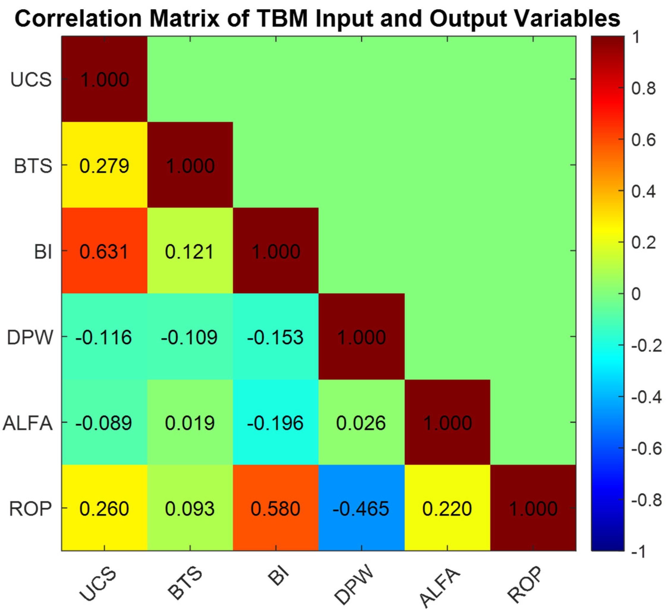
In the modeling process, BI, UCS, α, BTS, and DPW parameters were considered as independent variables, while the rate of penetration (ROP), representing the excavation performance, was designated as the dependent variable.

Although outlier removal is commonly applied to enhance model performance, in this study, extreme values were deliberately retained. Eliminating these data points could weaken the representation of natural excavation behavior in both hard and soft ground conditions. Therefore, the dataset was preserved in its entirety to ensure a more realistic reflection of actual field performance.

Additionally, the dataset was divided into two subsets, with 70% used for training and 30% for testing. In contrast to the commonly adopted 80–20 split in the literature, this study intentionally trained the model with a smaller portion of the data. This approach aimed to evaluate the model’s generalization capability under limited training conditions and to obtain a performance assessment that better reflects real-world scenarios. Remarkably, despite being trained with less data, the proposed model achieved superior predictive accuracy compared to studies employing larger training ratios, demonstrating its strong generalization ability and the effectiveness of the adopted methodology. This confirms that the SVM-based approach can effectively capture underlying patterns and maintain robust predictive power even when trained on a reduced dataset.

3.3. SVM Model

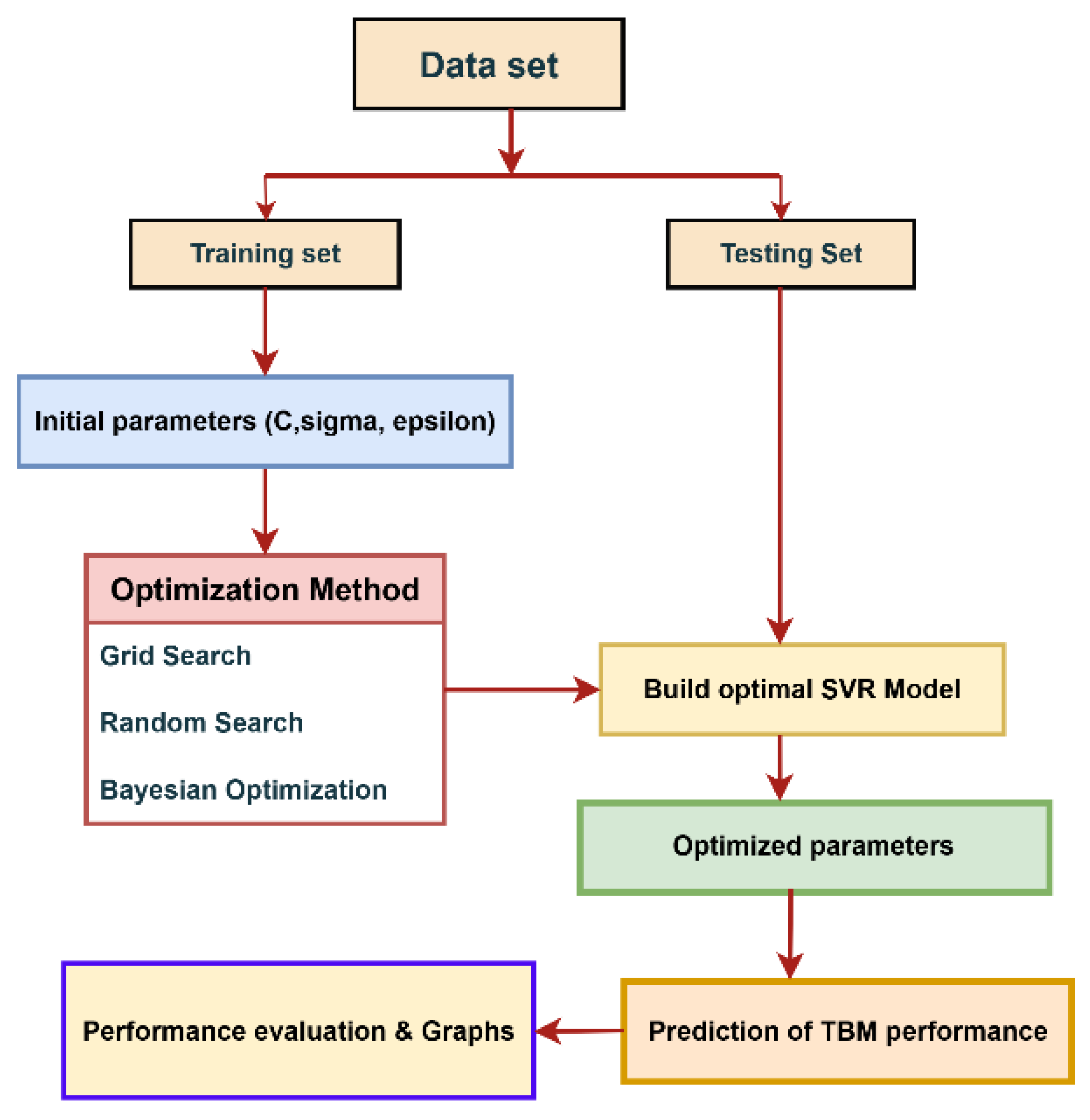
SVM is a powerful regression and classification technique capable of modeling both linear and nonlinear relationships. Since this study does not involve classification, SVR was employed to predict the TBM performance parameters. The flowchart of the SVR model is presented in Figure 3.

The SVR model illustrated in Figure 3 was configured using the Radial Basis Function (RBF) kernel, which enables effective learning by mapping nonlinear patterns into a high-dimensional feature space. The RBF kernel evaluates the similarity between data points based on Euclidean distance, allowing the model to capture complex structural relationships within the data. The performance of the SVR model is highly dependent on the proper selection of its key hyperparameters—C (penalty parameter), γ (gamma), and ε (epsilon).

Specifically, C governs the balance between model complexity and error tolerance, where higher values enforce stricter minimization of deviations and lower values offer greater model flexibility. The γ parameter determines the influence radius of the RBF kernel; smaller values yield smoother decision surfaces, whereas larger values create more localized and sharply defined regions. The ε parameter defines the width of the error-insensitive tube within which deviations are not penalized.

Because predictions in the SVR framework rely solely on support vectors, the model remains computationally efficient, requires relatively low memory, and maintains strong generalization capability. Additionally, the margin-maximization principle helps reduce the risk of overfitting.

In this study, the modeling procedure was conducted in three main stages. First, the SVR model was trained using the training dataset. Subsequently, the hyperparameters were optimized using Grid Search, Random Search, and Bayesian Optimization techniques. Finally, the optimal parameter combination was applied to the test dataset, and the predictive performance of the model was comprehensively evaluated.

3.4. Hyperparameter Optimization

The performance of an SVM model depends on three key parameters: the penalty parameter (C), the RBF kernel parameter (γ), and epsilon (ε) [15,19].

In this study, the hyperparameter ranges used in the SVR model were determined based on recommendations from previous research as well as preliminary experiments. The parameter C was defined within the range of 0.1–10,000 to balance model complexity and generalization capability, while γ, which controls the influence of individual training samples in capturing nonlinear relationships, was restricted to the interval between 1 × 10⁻⁶ and 0.1. The ε parameter, representing the tolerance for prediction errors, was explored within the range of 1 × 10⁻³ to 0.2. These ranges guided the hyperparameter search across the three optimization methods.

Hyperparameter optimization was performed using three different search strategies. Grid Search systematically evaluated all possible parameter combinations arranged on a logarithmically spaced grid within the selected ranges. Random Search tested 1000 randomly selected parameter combinations, enabling exploration of a broader parameter space with lower computational cost [33]. Bayesian Optimization was implemented as a probabilistic optimization technique that dynamically explores the parameter domain using a Gaussian Process-based surrogate model and selects new candidate combinations via the Expected Improvement (EI) acquisition function [34,35]. The performance of the SVM model depends on three key parameters: the penalty parameter (C), the RBF kernel parameter (γ), and epsilon (ε) [22,23].

4. Model Implementation

4.1. Machine Learning Algorithms

Machine learning is an artificial intelligence discipline that aims to mathematically represent complex processes and to generalize from past observations without requiring any predefined functional form, equation, or parametric structure. Instead, it derives patterns and relationships directly from data. This capability allows computer systems to learn how to perform a given task without being explicitly programmed to do so [36,37]. Machine learning algorithms are commonly categorized as supervised, unsupervised, or semi-supervised learning, and they can be applied to a wide range of problems, including regression, classification, clustering, and dimensionality reduction. Today, owing to their high predictive performance, flexibility, and minimal dependence on strict model assumptions, they have become essential analytical tools across numerous fields—from engineering and hydrology to medicine and financial modeling.

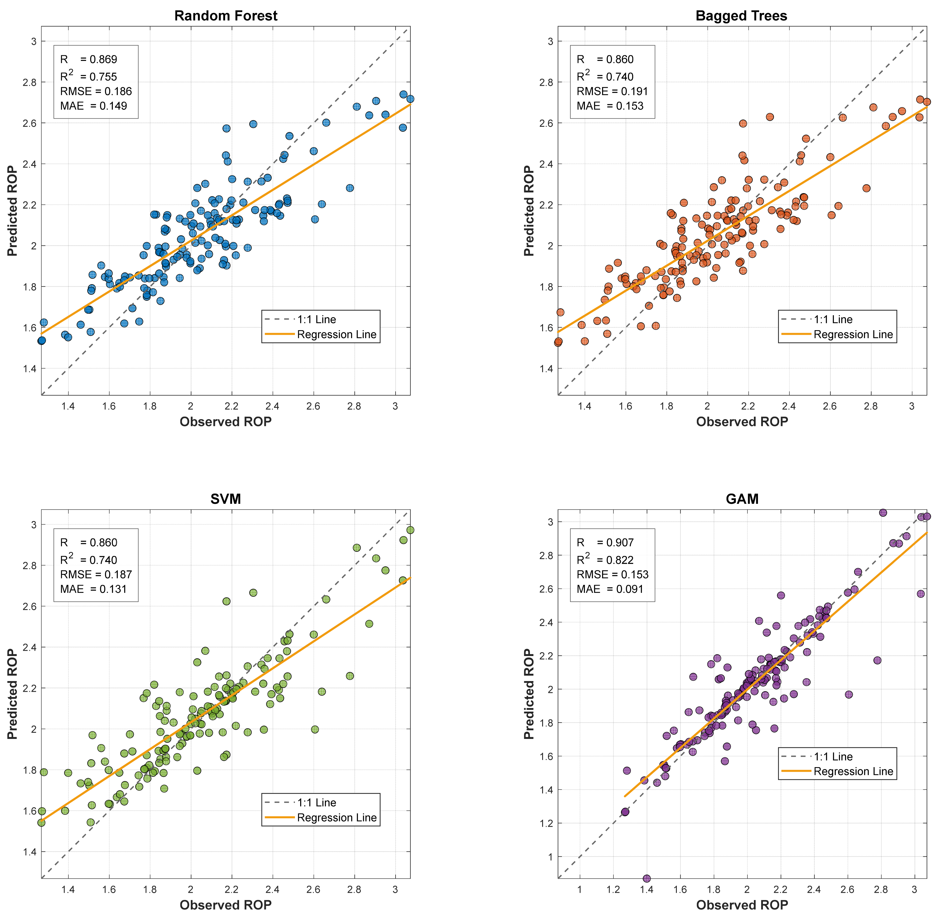
In this study, the predictive performance of the Support Vector Regression (SVR) method in estimating TBM penetration rate was evaluated through a comparative modeling framework using the same dataset. The SVR model was benchmarked against several classical machine learning algorithms, namely Random Forest (RF) [38,39], Bagged Trees (BT) [40], and the Generalized Additive Model (GAM) [41,42]. The quantitative performance indicators of these ML models are presented in

Table 1. Model Performance Comparison of Machine Learning Methods.

Model	R2	RMSE	MAE	RSR	NSE
RF	0.731	0.186	0.149	0.517	0.731
BT	0.717	0.191	0.153	0.531	0.717
SVM	0.728	0.187	0.131	0.520	0.728
GAM	0.819	0.153	0.091	0.425	0.819

, while Figure 4 illustrates scatter plots showing the relationships between observed and predicted values.

According to Table 1, the GAM outperforms the other methods across all performance metrics and achieves the highest predictive accuracy. RF and SVM models show comparable and moderately high performance, whereas BT ranks below them with a relatively lower level of accuracy. These findings are also clearly reflected in Figure 4, where the positions of the 1:1 and regression lines, together with the distribution of the scatter points, visually confirm the relative performance differences.

Sensitivity Analysis of Machine Learning Algorithms

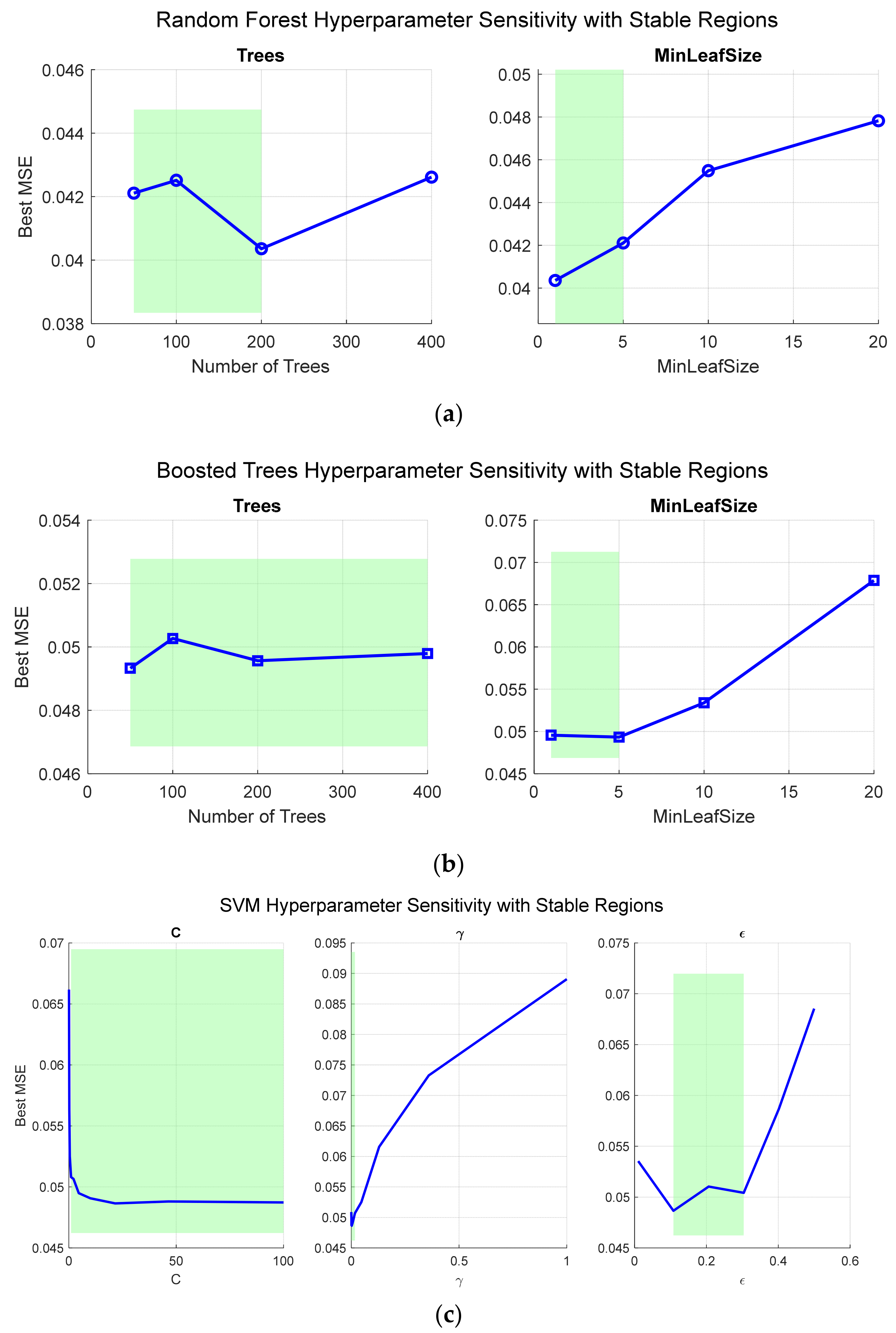
In this study, the developed code aims to systematically evaluate regression models based on Support Vector Machine (SVM), Random Forest (RF), Boosted Trees (BT), and Generalized Additive Model (GAM) using the same dataset. For the SVM model, the penalty parameter (C), kernel function parameter (γ), and error tolerance parameter (ε) were defined over different ranges, and each hyperparameter combination was assessed using five-fold cross-validation, with the corresponding mean squared error (MSE) values calculated. Similarly, for the RF and BT models, the effects of the number of trees and the minimum leaf size on model performance were investigated, and prediction errors were obtained for each hyperparameter combination using the test dataset.

Through this approach, the optimal hyperparameters for each model were identified, and the relative influence of individual hyperparameters on predictive performance was quantified. In addition, a computational cost analysis was conducted for all models by separately measuring and comparing training and prediction times. Consequently, not only prediction accuracy but also computational efficiency and practical applicability of the models were evaluated, and the results are presented in Figure 5.

The stability region analyses presented in Figure 5 reveal the hyperparameter sensitivities and performance tolerances of different machine learning models. In SVM, the γ parameter of the RBF kernel exhibits a narrow stable range with high performance sensitivity; even small changes can significantly affect the mean squared error (MSE). In contrast, the C parameter has a broader stable range, and ε shows an intermediate range, making γ tuning critical while providing more tolerance for C and ε. In Random Forest and Boosted Trees models, the number of trees is relatively tolerant, whereas the MinLeafSize parameter requires careful adjustment.

GAM was primarily evaluated for interpretability, with partial dependence functions directly visualizing the effect of each input on ROP. Some variables display linear relationships, while others exhibit nonlinear and saturation effects. Computationally, SVM and GAM offer shorter training times, whereas Boosted Trees require the longest; prediction times are fast across all models. These findings enable a comparative assessment of the models in terms of both performance and computational efficiency, supporting their applicability in decision-making processes.

4.2. Optimized SVR Model

In this study, the developed SVM model was implemented using three different optimization strategies after splitting the dataset into 70% training and 30% testing, as illustrated in Figure 3. The predictive performance of the model was comprehensively evaluated using several performance indicators, including Mean Absolute Error (MAE), Mean Squared Error (MSE), Root Mean Squared Error (RMSE), the Coefficient of Determination (R²), and the Nash–Sutcliffe Efficiency Coefficient (NSE).

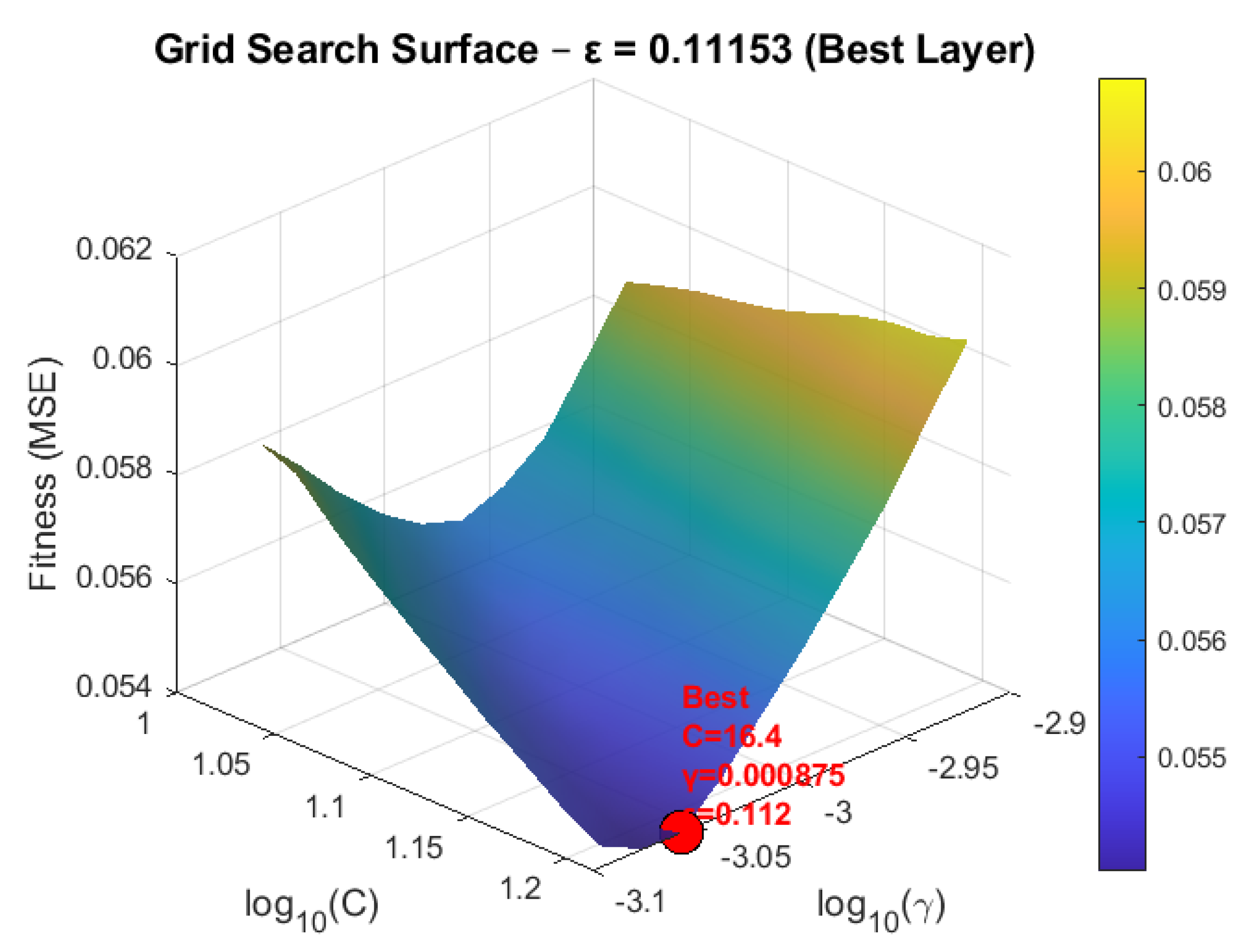
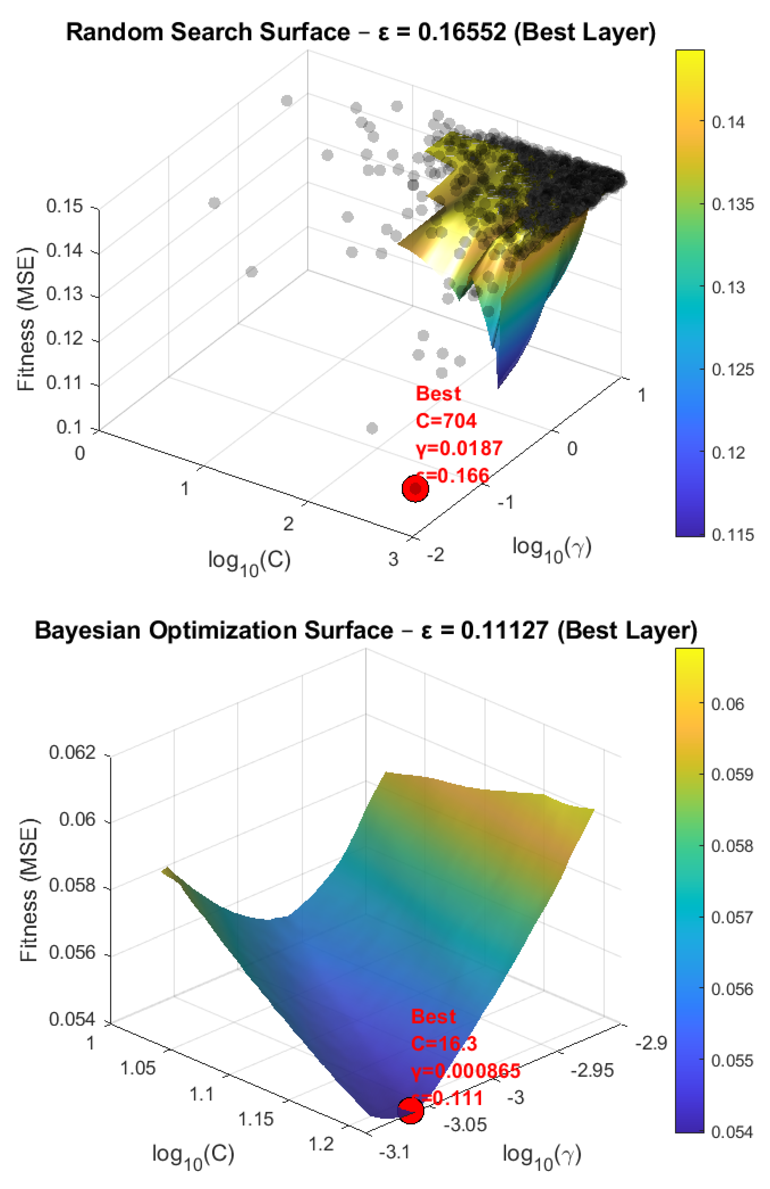
During the hyperparameter optimization phase, Grid Search, Random Search, and Bayesian Optimization techniques were employed. Among these methods, Bayesian Optimization demonstrated a clear advantage in terms of computational efficiency by achieving high prediction accuracy with significantly fewer evaluations. The optimal values of C and γ obtained from each technique reflected the distinct search behaviors of the optimization methods, and the impact of these variations on model performance was visualized through the three-dimensional hyperparameter search surfaces shown in Figure 6.

These visualizations clearly indicate that Bayesian Optimization reaches optimal performance with a limited number of evaluations and provides more efficient hyperparameter tuning compared with Grid Search and Random Search. While Grid Search yielded results close to those of Bayesian Optimization, Random Search exhibited greater deviations from the optimal region.

Although reducing grid density in Grid Search or increasing the number of iterations in Random Search could potentially enhance model performance, both approaches substantially increase computational time and memory requirements. In contrast, Bayesian Optimization offers a distinct advantage by delivering high predictive accuracy and computational efficiency with far fewer evaluations.

Overall, the predictions derived from the measured data demonstrate that the developed model exhibits high accuracy and stability. Furthermore, the comparative analysis of the optimization strategies highlights the critical role of hyperparameter selection in model performance and provides a practical methodology for engineering applications that aim to achieve effective results under limited computational resources.

As shown in Figure 6, the optimal SVR parameters obtained through Bayesian Optimization were determined as C = 16.322462, γ = 0.000865, and ε = 0.111265. To examine the effect of these parameters on model performance, SVR models constructed using parameter sets obtained from the Grid Search and Random Search methods were evaluated and compared using the MSE, RMSE, MAE, NSE, and R² metrics. All computations were performed on a 64-bit computer running the Windows operating system, equipped with a 12th-generation Intel Core i7-12700H processor (2.30 GHz) and 32 GB of RAM. The results for the training, test, and entire datasets are presented in

Table 2. Comparison of SVR parameter optimization methods and model performance.

Opt. Method	Opt. Parameters	Dataset	CPU (s)	MSE	MAE	RMSE	R2	NSE
Bayesian	C = 16.32	Training	17.31	0.0096	0.0927	0.0981	0.9610	0.9194
	γ = 0.000865	Testing		0.0121	0.1099	0.1100	0.9625	0.9231
	ε = 0.111	All		0.0101	0.0961	0.1006	0.9607	0.9213
Random Search	C = 704	Training	19.19	0.0197	0.1301	0.1404	0.9277	0.8534
	γ = 0.0187	Testing		0.0214	0.1409	0.1462	0.8709	0.7951
	ε = 0.166	All		0.0201	0.1323	0.1416	0.9183	0.8440
Grid Search	C = 16.4	Training	25.83	0.0102	0.0967	0.1010	0.9558	0.9159
	γ = 0.000875	Testing		0.0106	0.0974	0.1030	0.9726	0.9268
	ε = 0.112	All		0.0103	0.0968	0.1014	0.9600	0.9200

. In addition, Table 2 reports the number of function evaluations (NFE) required during model training, as well as the required CPU time in seconds.

As presented in Table 2, the R² values for the training and test datasets were obtained as 0.9610 and 0.9625, respectively, while the NSE values were 0.9164 and 0.9231, and the MAE values were 0.0927 and 0.1099. These results indicate minimal prediction errors and demonstrate that the SVM model exhibits high accuracy and strong predictive capability. In addition, the comparatively lower-performing Random Search and Grid Search results still fall within the range of 0.75 ≤ NSE (0.9231, 0.7951, 0.9275) ≤ 1, corresponding to the “Very good” classification according to the criteria reported in reference [43]. While the performance of Grid Search was found to be close to that of Bayesian Optimization, Random Search yielded comparatively lower predictive accuracy.

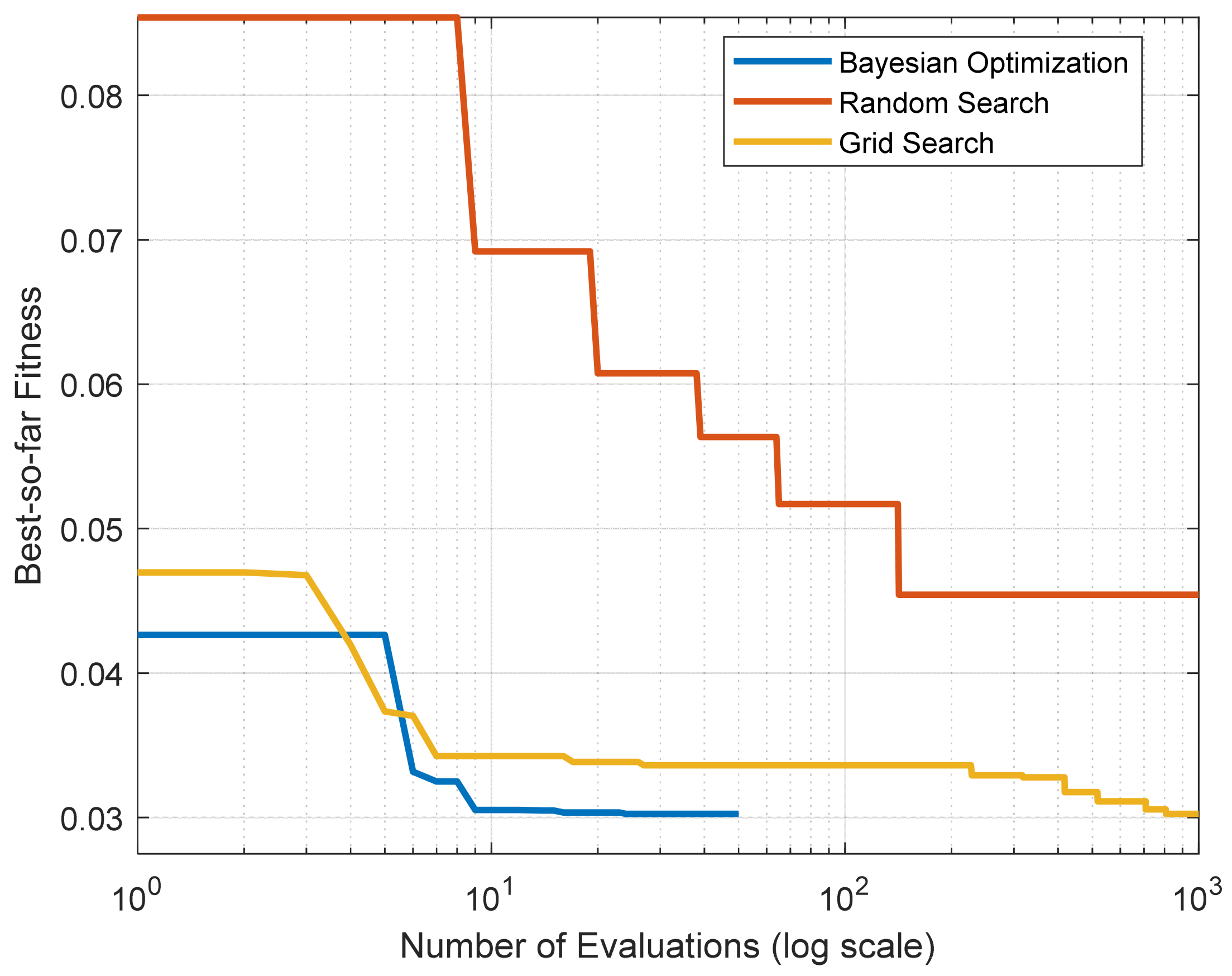
The convergence curves of the three optimization strategies used for SVR parameter tuning, with respect to the number of function evaluations, are presented in Figure 7. As shown in Figure 7, the Bayesian optimization algorithm reaches a stable solution after approximately 30 evaluations, whereas the Grid Search algorithm requires about 1000 function evaluations to achieve similar performance, and Random Search generally exhibits lower performance than the other two methods even after 1000 trials. These results indicate that the proposed Bayesian optimization approach is highly efficient for the SVR model, achieving optimal parameters with a limited number of iterations (30–50). In terms of computational time, as shown in Table 2, Grid Search requires 25.83 s, while Bayesian optimization completes in 17.31 s. In other words, Bayesian optimization is more advantageous in terms of model performance, number of iterations, and CPU time.

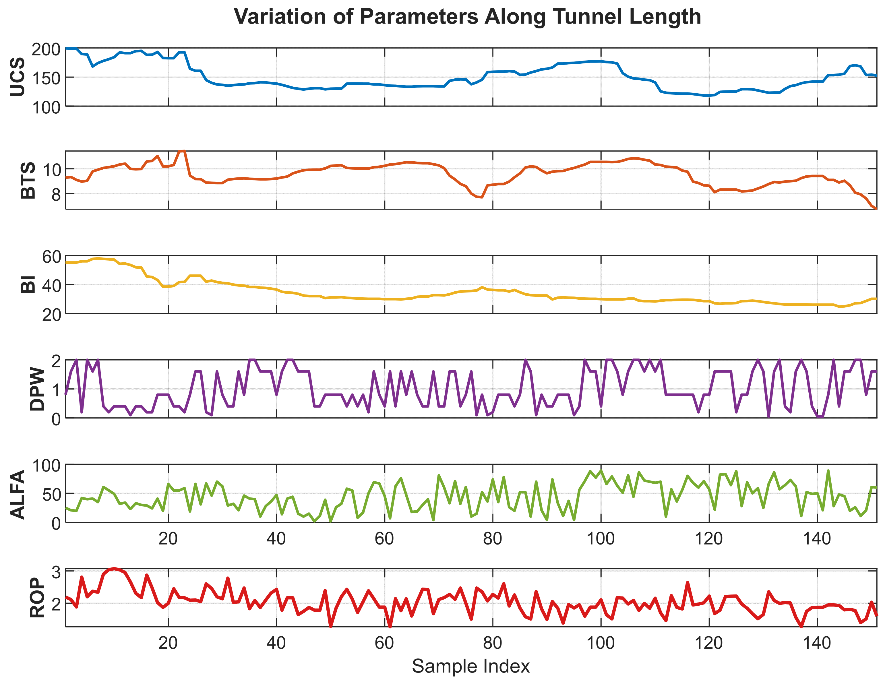
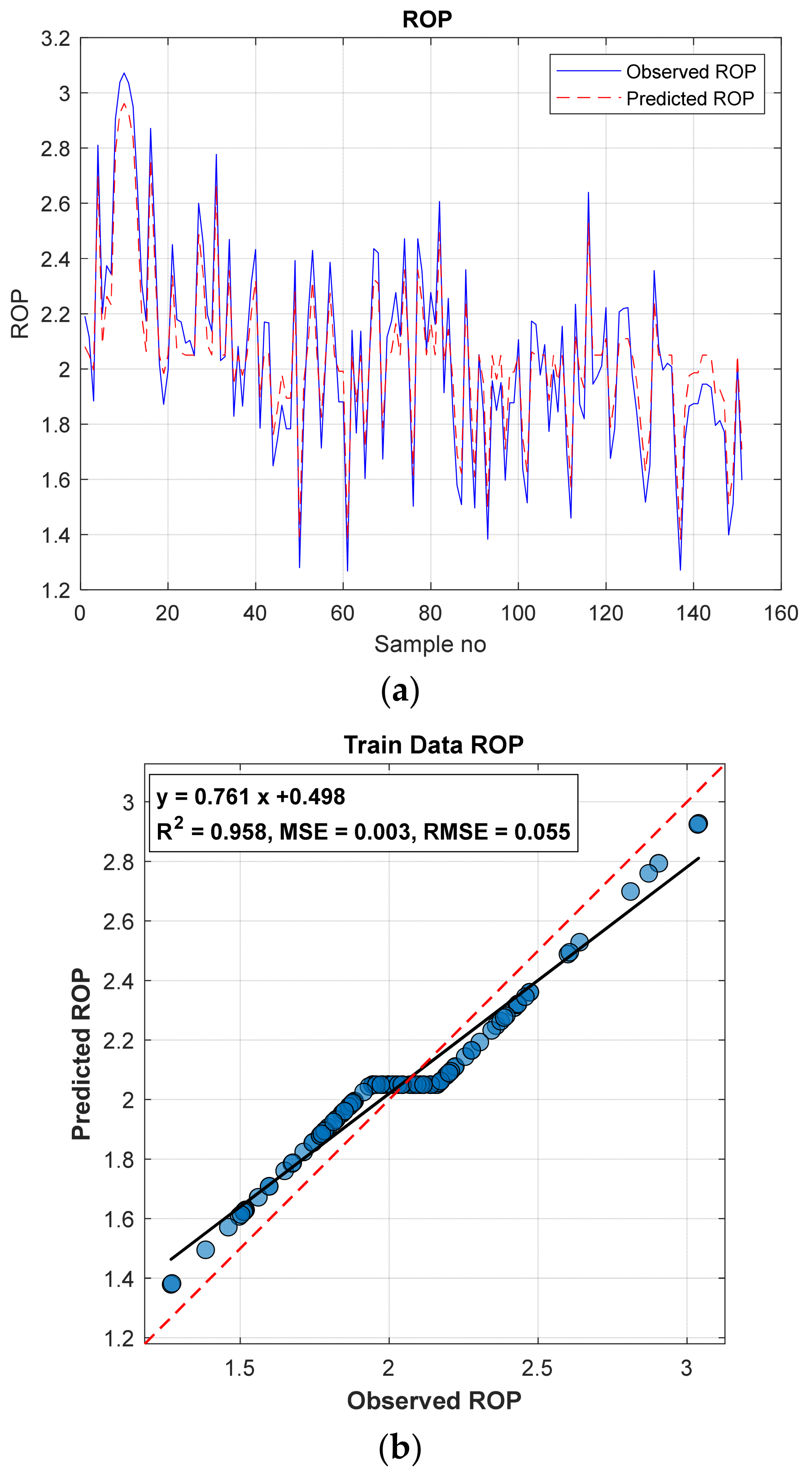
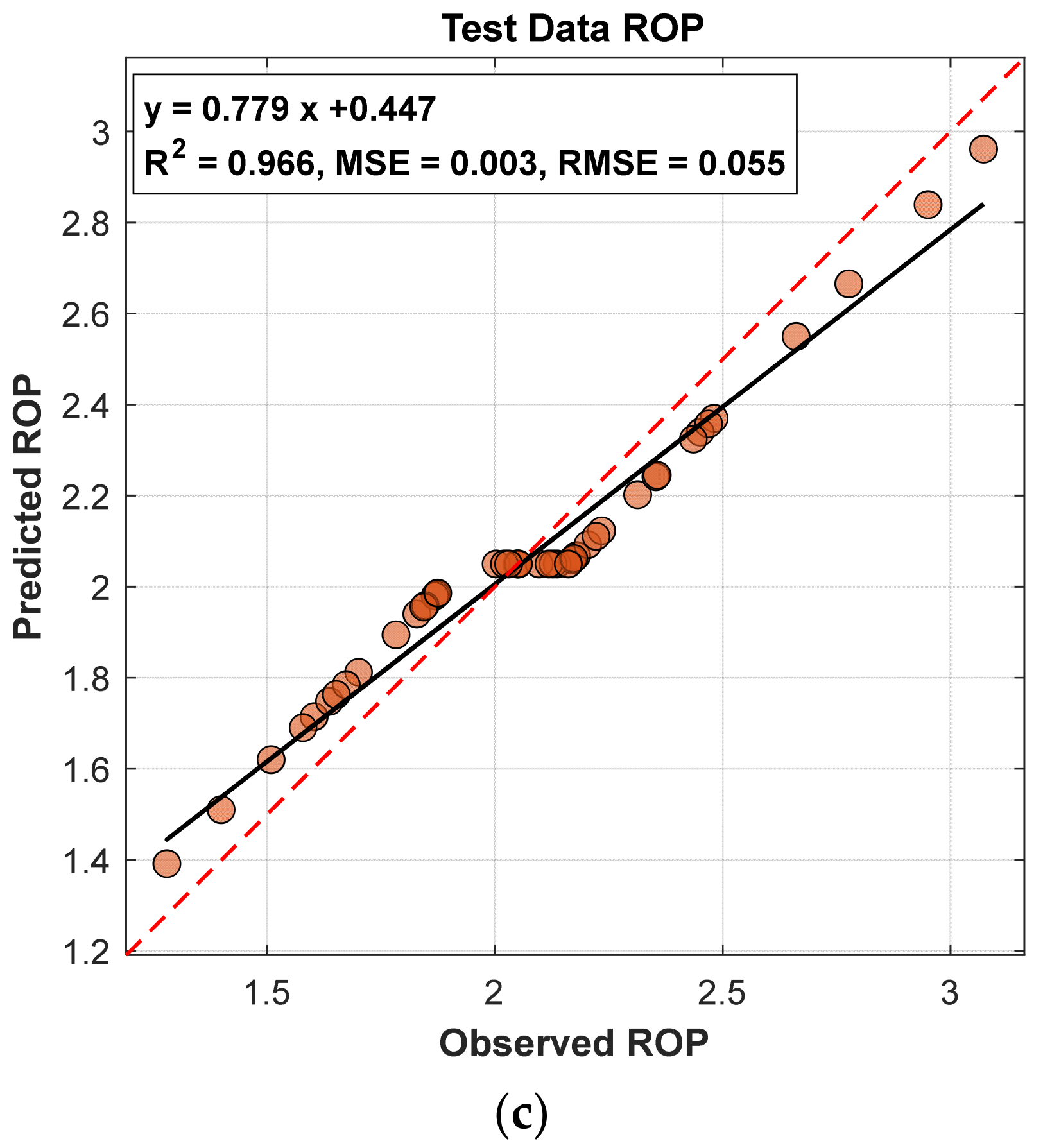
Figure 8 illustrates (a) the ROP predictions along the tunnel, (b) the distribution of the training data, and (c) the distribution of the test data.

When Table 2 and Figure 8 are evaluated together, it is evident that the model maintains high accuracy and stability across both datasets, and the predictions exhibit a strong agreement with the observed values.

4.3. Feature Importance Analysis

Feature importance analysis is a fundamental explainability approach that reveals the extent to which a machine learning model relies on each input variable when predicting the target output. In scientific studies, this analysis is crucial not only for demonstrating how well a model performs but also for identifying which variables contribute to this performance. The literature emphasizes that feature importance—particularly in tree-based methods such as Random Forest and Gradient Boosting—is a powerful tool for understanding a model’s decision-making mechanism and plays an essential role in interpretability, reliability, and decision-support processes [38,40].

The primary objective of determining feature importance is to clarify the relative impact of the variables in the dataset and enhance the transparency of the model’s internal operations. Through this analysis, it becomes evident which inputs the model relies on most and which variables contribute most significantly to prediction accuracy. As a result, the model moves away from being a “black box” and becomes more interpretable to users. Since not all inputs contribute equally in multivariate data structures, identifying truly informative variables and separating them from noise becomes possible only through such analyses.

Feature importance analysis also offers substantial advantages in terms of dimensionality reduction and model simplification. Removing variables with low contribution, redundancy, or high collinearity leads to a more concise model structure, shortens training time, reduces computational cost, and improves generalization performance. The literature indicates that effective feature selection reduces the risk of overfitting and makes models more robust against independent test data [44].

Additionally, evaluating feature importance facilitates comparisons across different models. Observing which variables receive higher emphasis in different algorithms applied to the same dataset enables an understanding of the learning dynamics and sensitivities of each model. When a specific physical or biophysical variable exhibits high importance in a model, it indicates that the model is more responsive to that process. This not only enables statistical interpretation but also offers process-based insights, providing valuable scientific contributions, particularly in disciplines such as remote sensing, geosciences, hydrology, and environmental modeling.

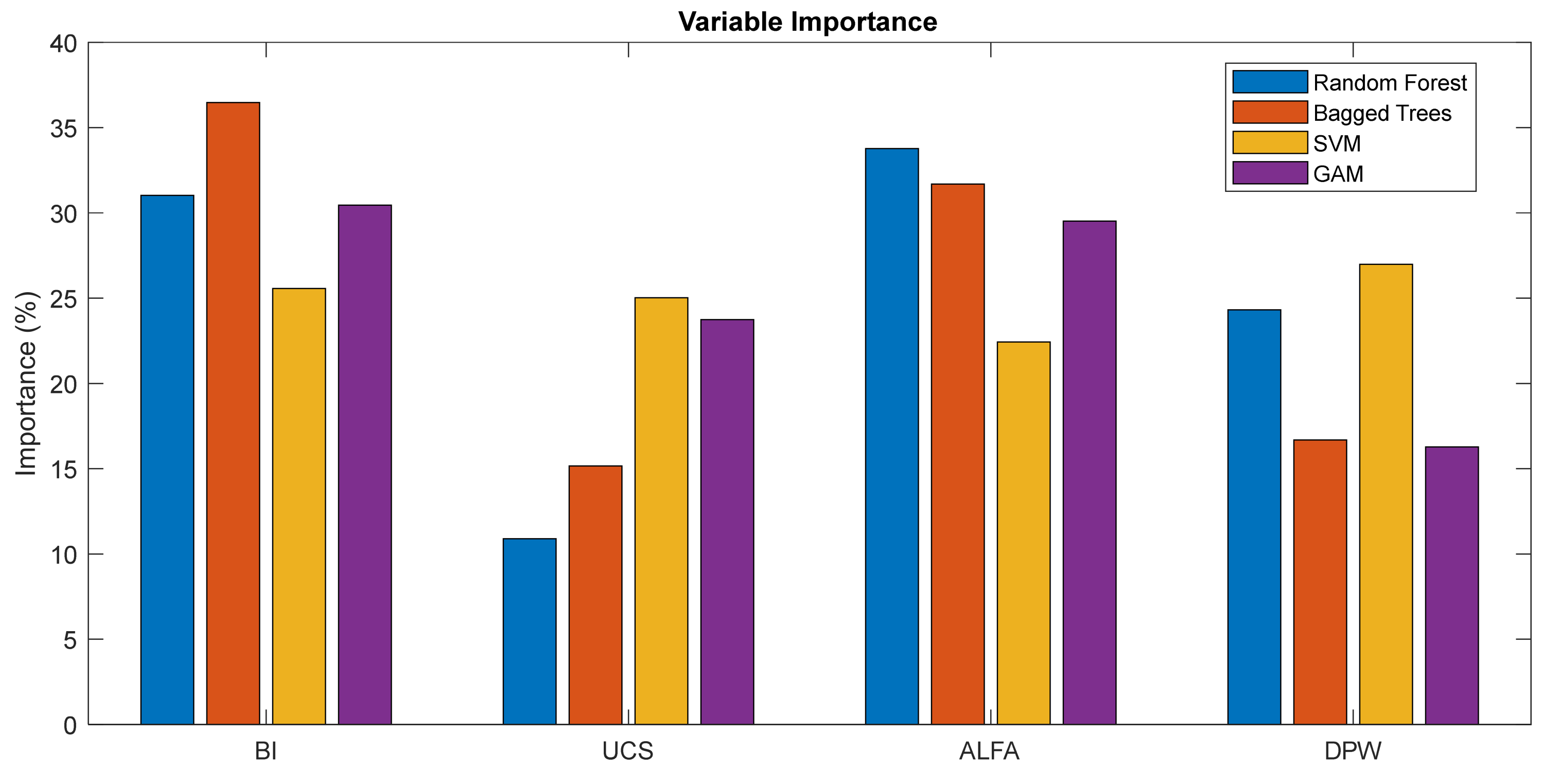
For these reasons, this study presents—for the first time in TBM performance modeling—a detailed investigation of the influence of input variables on ROP using four different machine learning approaches. The analysis results are presented in

Table 3. Model-Based Variable Importances for ROP Prediction.

ML Method	Variable
	BI	UCS	ALPHA	DPW
RF	31.03	10.89	33.77	24.31
BT	36.47	15.17	31.68	16.68
SVM	25.56	25.03	22.43	26.98
GAM	30.45	23.74	29.52	16.28

and Figure 9.

Table 3 presents a comparative overview of the relative importance of the input variables across four different machine learning methods used for ROP prediction (RF, BT, SVM, and GAM). The results indicate that variable importance varies distinctly between models, reflecting the differing sensitivities of each algorithm to the underlying data structure.

Tree-based methods (RF and BT) identified BI and ALPHA as the most influential variables. In the RF model, ALPHA (33.77%) and BI (31.03%) emerged as the dominant predictors, whereas BT highlighted BI (36.47%) as the primary variable. This suggests that tree-based methodologies are particularly sensitive to physical and geometric parameters related to penetration in the context of ROP prediction.

Unlike the tree-based algorithms, the SVM model distributed variable importance more evenly among the inputs, with BI, UCS, ALPHA, and DPW showing comparable contributions. Notably, the relatively high importance of UCS in SVM (25.03%) indicates that nonlinear, kernel-based approaches tend to assign greater relevance to strength-related properties of the rock mass.

The GAM, on the other hand, assigned similar importance levels to BI (30.45%), ALPHA (29.52%), and UCS (23.74%), while attributing lower importance to DPW. This pattern highlights GAM’s semi-parametric flexibility in capturing smooth and gradual variations in predictor effects, consistently emphasizing the BI–ALPHA–UCS trio.

Overall, the findings show that BI and ALPHA are dominant predictors of ROP across all four models, whereas the importance of DPW varies considerably between methods. UCS, meanwhile, plays a more substantial explanatory role in GAM and SVM. These differences arise from the distinct ways in which each algorithm perceives and interprets relationships within the data, reinforcing that ROP prediction is a multidimensional problem sensitive to interactions among multiple parameters.

In conclusion, feature importance analysis is not merely a model performance assessment tool; it is a comprehensive approach that enhances model interpretability, supports performance optimization, provides deeper insight into variable–target relationships, and strengthens the scientific reliability of the results. The motivation behind conducting this analysis is not only to evaluate model accuracy but also to elucidate the foundations on which the model operates—thereby contributing meaningfully to both practical applications and the academic literature.

5. Discussion

The SVM model developed in this study demonstrated both high accuracy and remarkable stability in predicting the rate of penetration (ROP) during tunnel excavation. The performance metrics presented in Table 2 clearly indicate strong agreement between the predicted and observed values for both the training and test sets: the R² values were 0.9610 and 0.9625, NSE values were 0.9194 and 0.9231, and MAE values were 0.0927 and 0.1099, respectively. The training and test MSE values (0.0096 and 0.0121) are both very low and close to each other, providing strong evidence of the model’s high generalization capability and absence of overfitting.

Fattahi and Babanouri [45] also employed a similar SVR model; however, they optimized the model parameters using a hybrid framework incorporating heuristic algorithms such as Differential Evolution (DE) [46], Artificial Bee Colony (ABC) [47], and the Gravitational Search Algorithm (GSA) [48]. In contrast, the present study performed hyperparameter tuning as a sequential search procedure, applying Grid Search, Random Search, and Bayesian Optimization consecutively, and selecting the optimal parameters obtained from the best-performing method. The SVR model trained with these optimized parameters exhibited significant improvements in test performance and enhanced consistency between training and test predictions. Therefore, compared to [45], the performance difference largely stems from the optimization strategy employed, indicating a stronger generalization capacity in the current model.

When comparing the two SVR configurations developed using the same dataset, the optimized parameter set obtained through the Grid–Random–Bayesian sequence in this study (C = 16.32, γ = 0.000865, ε = 0.111) provides a lower complexity structure with a broader influence range, making it more robust to noise and yielding superior generalization capability. On the other hand, the parameter set reported in [45] (C = 2605.86, γ ≈ 0.067, ε = 0.214) contains an excessively large C value and a comparatively higher γ, which makes the model overly sensitive to the training data, increases the risk of overfitting, and ultimately limits its generalization performance.

Meanwhile, studies such as [22,23] and Afradi et al. [24] used different datasets and methodologies; therefore, performance comparisons can only be interpreted at a methodological level rather than directly. For instance, the SVR model developed in [22] using the Queens Water Tunnel dataset achieved high R² values of 0.99 for training and 0.95 for testing. However, the limited sample size and the use of eight input variables restricted the model’s ability to generalize across varying geological conditions. Similarly, [23] compared ANN, SVM, and GEP models, reporting relatively lower performance for SVM. In these studies, SVR parameters were set as C = 1000, σ = 0.5 (γ = 2), and ε = 0.1 in [23,24], while in [22], ε was set to 0.1 and the other two parameters were determined through 10-fold cross-validation via trial-and-error. In other words, none of these studies employed a systematic optimization procedure for determining SVR hyperparameters.

To evaluate the impact of optimal SVR parameter selection on model performance, the parameter set reported in [45] (C = 2605.86, γ = 0.067, ε = 0.111) was applied to the same dataset using the SVR algorithm of the present study, and the resulting performance metrics were recalculated. A summary of the results is presented in

Table 4. Comparative results demonstrating the impact of optimal SVR parameters on model performance.

Reference	Opt. Method	Dataset	MSE	MAE	RMSE	R2	NSE
[45]	SVR-DE	Training	0.0302	0.1600	0.1737	0.8599	0.7549
		Testing	0.0299	0.1540	0.1730	0.9100	0.7836
		All	0.0301	0.1588	0.1736	0.8728	0.7655
This study	Bayesian	Training	0.0102	0.1008	0.0968	0.9164	0.9583
		Testing	0.1016	0.1008	0.0950	0.9292	0.9664
		All	0.0102	0.1008	0.0963	0.9209	0.9605

.

Examination of Table 4 shows that the optimal SVR parameters obtained through Bayesian optimization provide substantial improvements over those used in [45] across all performance metrics for the training, test, and complete datasets. In particular, the reductions in MSE, MAE, and RMSE, together with the increases in R² and NSE, clearly demonstrate that hyperparameter optimization significantly enhances the predictive capability of the SVR model.

Bayesian optimization reached the optimal parameter set within approximately 30–50 function evaluations, whereas Grid Search required nearly 1000 evaluations to achieve comparable results. Moreover, Bayesian optimization improved the test performance to R² = 0.97 while demonstrating superior efficiency in terms of the number of function evaluations and CPU time compared to the RS and GS algorithms. Consequently, the three optimization algorithms were applied sequentially, their results compared, and the optimal parameters yielding the highest model performance were selected for the final SVR model.

Although the influence of SVR hyperparameters may vary depending on the characteristics of the dataset, general tendencies are well established: γ strongly affects model complexity by controlling the effective radius of the RBF kernel; C adjusts the penalty for errors, thereby governing the model’s flexibility; and ε defines the width of the insensitive zone, affecting the number of support vectors to a limited extent.

A key contribution of this study is the integrated treatment of the dataset, model inputs, and hyperparameter optimization strategy. The high R² and NSE values, along with very low RMSE and MAE values, demonstrate the model’s robustness and strong generalization capability. Future studies may further enhance generalization performance by applying k-fold cross-validation.

As shown in Table 1, although baseline SVM performance is comparable to RF and BT, the SVR model exhibits significant improvements across all metrics once its hyperparameters are optimized using the proposed strategies. For example, the R² value increases from 0.728 to 0.966, while the MAE decreases from 0.131 to 0.095, clearly illustrating that carefully tuned hyperparameters are critical for improving model accuracy and stability.

A detailed examination of hyperparameter effects not only provides methodological insight for academic research but also facilitates the development of more reliable and computationally robust SVM models for TBM applications.

In conclusion, the comprehensive analysis of feature importance demonstrates that the contribution of this study extends beyond predictive performance, providing significant value for understanding underlying physical processes and for developing interpretable, engineering-relevant prediction frameworks. The findings offer both a methodological reference for future research and a practical basis for more reliable, computationally efficient, and physically meaningful TBM performance predictions.

6. Conclusions and Future Work

In this study, an SVM-based model was developed to predict the rate of penetration (ROP) during tunnel excavation, and hyperparameter optimization was systematically carried out using Grid Search (GS), Random Search (RS), and Bayesian Optimization (BO). The results indicate that BO reached the optimal parameter set with only 30–50 evaluations, whereas GS and RS required approximately 1000 evaluations. In addition, BO achieved the highest predictive accuracy (R² = 0.9625) while reducing the computational time from 25.83 s (GS) to 17.31 s. Compared with the baseline SVM model, the optimized SVR demonstrated high accuracy (R² = 0.9610–0.9625), strong stability (NSE = 0.9194–0.9231), and low error levels (MAE = 0.0927–0.1099), clearly highlighting the critical role of hyperparameter optimization in improving model performance.

One of the key contributions that distinguishes this study from previous work in the literature is not only the systematic execution of hyperparameter optimization but also the detailed examination of Model-Based Feature Importances. The variable importance values presented in Table 3 consistently indicate that BI, ALPHA, and DPW are the most influential parameters on ROP. This finding aligns with the physical processes governing the excavation mechanism and demonstrates that the model successfully captures the causal relationships within the data. Moreover, the relatively higher importance of UCS in the SVM and GAM highlights the deterministic influence of strength parameters. The similarity of feature importance trends across different models confirms that the prediction process is both mathematically and physically coherent.

Therefore, this study demonstrates that combining hyperparameter optimization with feature importance analysis enables the development of more reliable and interpretable models for TBM penetration rate prediction. This holistic approach not only provides a methodological reference for academic research in geotechnical engineering but also establishes a robust predictive framework for practical applications.

Future studies will aim to enhance the generalization capacity of the model by using larger and more up-to-date datasets representing different geological conditions and excavation machines. In addition, investigating how variable importances change across different geological environments will further strengthen the interpretability of SVM and other machine learning models.