Article

Semantic-Guided Spatial and Temporal Fusion Framework for Enhancing Monocular Video Depth Estimation


Department of Computer Science and Artificial Intelligence, Dongguk University, Seoul 04620, Republic of Korea
*
Authors to whom correspondence should be addressed.
Appl. Sci. 2026, 16(1), 212; https://doi.org/10.3390/app16010212
Submission received: 25 November 2025 / Revised: 16 December 2025 / Accepted: 23 December 2025 / Published: 24 December 2025
(This article belongs to the Special Issue Advances in Computer Vision and Digital Image Processing)

Abstract

Despite advancements in deep learning-based Monocular Depth Estimation (MDE), applying these models to video sequences remains challenging due to geometric ambiguities in texture-less regions and temporal instability caused by independent per-frame inference. To address these limitations, we propose STF-Depth, a novel post-processing framework that enhances depth quality by logically fusing heterogeneous information—geometric, semantic, and panoptic—without requiring additional retraining. Our approach introduces a robust RANSAC-based Vanishing Point Estimation to guide Dynamic Depth Gradient Correction for background separation, alongside Adaptive Instance Re-ordering to clarify occlusion relationships. Experimental results on the KITTI, NYU Depth V2, and TartanAir datasets demonstrate that STF-Depth functions as a universal plug-and-play module. Notably, it achieved a 25.7% reduction in Absolute Relative error (AbsRel) and significantly enhanced temporal consistency compared to state-of-the-art backbone models. These findings confirm the framework’s practicality for real-world applications requiring geometric precision and video stability, such as autonomous driving, robotics, and augmented reality (AR).

1. Introduction

Monocular Depth Estimation (MDE) is a fundamental task in computer vision, aiming to predict dense depth maps from a single RGB image. It serves as a critical component in various applications, including autonomous driving, robotics, and augmented reality (AR), where understanding the 3D geometry of a scene is essential. With the advent of deep learning, MDE has achieved remarkable progress, evolving from early supervised methods to recent self-supervised and foundation model-based approaches [1,2,3].
Recently, deep learning techniques have extensively demonstrated their efficacy in image processing and analysis tasks. Empirical studies utilizing advanced architectures for complex vision tasks highlight the high accuracy and practicality of deep learning in unstructured environments [4,5,6]. This evidence strongly supports the validity of applying deep learning-based approaches to high-level vision tasks such as Monocular Depth Estimation (MDE).
However, despite these advancements, applying image-based MDE models directly to video sequences introduces significant challenges. Since standard MDE models perform inference on each frame independently, they often fail to maintain temporal consistency, leading to severe flickering artifacts. Furthermore, in texture-less regions such as roads or walls, MDE models frequently suffer from scale ambiguity and geometric distortions due to the lack of distinct visual features. While recent video-based depth estimation methods attempt to address these issues by leveraging temporal information across multiple frames [7,8], they typically require heavy computational resources or extensive retraining, limiting their flexibility as a general-purpose solution.
To address these limitations without the need for retraining or heavy architectural changes, we propose STF-Depth (Spatial-Temporal Fusion Depth), a novel post-processing framework designed to serve as a universal plug-and-play module. STF-Depth enhances the output of any off-the-shelf MDE model by logically fusing heterogeneous information—geometric constraints, semantic context, and instance-level details (Figure 1). Our approach introduces a robust RANSAC-based Vanishing Point (VP) Estimation to guide Dynamic Depth Gradient Correction, effectively resolving scale ambiguities in background regions. Additionally, we employ Adaptive Instance Re-ordering based on panoptic segmentation to clarify occlusion relationships and sharpen object boundaries. Finally, an efficient temporal fusion module ensures stability across video frames.
The main contributions of this paper are summarized as follows:
  • We propose STF-Depth, a training-free post-processing framework that significantly enhances the geometric accuracy and temporal stability of existing MDE models.
  • We introduce a Depth-Stratified Vanishing Point Estimation method combined with Semantic-Guided Spatial Fusion, which robustly corrects perspective distortions in complex environments.
  • Extensive experiments on the NYU Depth V2, KITTI, and TartanAir datasets demonstrate the effectiveness of our approach. Notably, STF-Depth achieved a 25.7% reduction in Absolute Relative error (AbsRel) and significantly improved temporal consistency compared to state-of-the-art backbone models.

2. Related Work

2.1. Monocular Depth Estimation

Monocular Depth Estimation (MDE), the task of estimating pixel-wise depth from a single image, has evolved significantly with the advent of Deep Learning. Early research primarily utilized CNN-based encoder-decoder architectures to treat depth estimation as a simple regression problem [1]; however, these methods often focused on local features, missing global context. To address this, recent approaches have adopted Vision Transformers (ViTs) to learn global dependencies across the entire image [9]. Notably, state-of-the-art models like MiDaS and the Dense Prediction Transformer (DPT) demonstrate robust generalization capabilities by “mixing datasets” during training, enabling them to generate high-quality depth maps across diverse indoor and outdoor environments rather than being limited to specific domains [10,11]. Furthermore, advancements in robust training frameworks under noisy labels, such as PSSCL [12], contribute to the increasing reliability of computer vision models.
In this study, these SOTA MDE models serve as the backbone without retraining, providing the initial depth values for our framework. However, since these models rely solely on textural and geometric features, they inherently suffer from “boundary mismatch” limitations, often failing to clearly distinguish semantic boundaries or blending foreground objects with the background. Therefore, instead of using their outputs as the final result, we utilize them as a “raw geometric source” to be fused with semantic segmentation information. This approach allows us to leverage the strong distance estimation capabilities of existing models while compensating for their geometric ambiguities using external semantic knowledge.

2.2. Semantic and Panoptic Segmentation

Image segmentation is a core technology for scene understanding in computer vision, classifying object classes at the pixel level. Semantic segmentation models, such as DeepLabV3, effectively separate foreground from background by capturing multi-scale context through mechanisms like atrous convolution [13]. More recently, this field has expanded to Panoptic Segmentation, which unifies semantic and instance segmentation [14]. Models like OneFormer simultaneously identify amorphous “stuff” regions (e.g., sky, road) and countable “thing” instances (e.g., person, car), assigning a unique ID and semantic meaning to every visual element in the image [15].
In this study, these segmentation models play a crucial role as guides for restructuring the spatial layout of depth maps. As illustrated in Figure 2, while the geometric source (b) generated by the depth estimation model provides “distance” information but lacks clear object boundaries, the semantic source (c) and panoptic source (d) generated by segmentation models precisely recognize “object shapes” and “individual instances” despite lacking depth data. We leverage these complementary characteristics of heterogeneous information to project the clear boundary information provided by segmentation models into the depth space, thereby restoring the morphological integrity of objects that depth models often miss.

2.3. Video Depth Estimation and Temporal Consistency

The major challenge in estimating depth from video sequences is the temporal inconsistency, or flickering, caused by processing each frame independently. Existing studies have largely addressed this by calculating Optical Flow to warp and align depth values between adjacent frames [16,17] or by introducing sequence models like ConvLSTM and Video Transformers to explicitly learn temporal correlations. For instance, ManyDepth [18] leverages multi-view geometry for self-supervised learning, while recurrent approaches like Recurrent Depth [19] integrate temporal information through memory units. Recently, foundation models trained on large-scale datasets, such as Video Depth Anything [20], have set new performance standards in consistent depth estimation. However, these methods typically incur prohibitive computational costs during inference, hindering real-time performance, or require the burden of retraining models on domain-specific video datasets [21,22,23].
In contrast, this study proposes an efficient Temporal Fusion strategy that eliminates the need for complex optical flow computations or retraining. Rather than simply blending pixels, our approach first secures spatial stability through geometry-aware constraints based on vanishing points and object attributes. This allows us to demonstrate that a relatively lightweight window-based temporal smoothing is sufficient to achieve robust temporal consistency. This presents a practical balance between computational efficiency and visual stability, offering a lightweight alternative to existing computationally intensive video depth estimation models. Table 1 summarizes the comparison between existing video depth estimation methods and our proposed framework.

3. Methodology

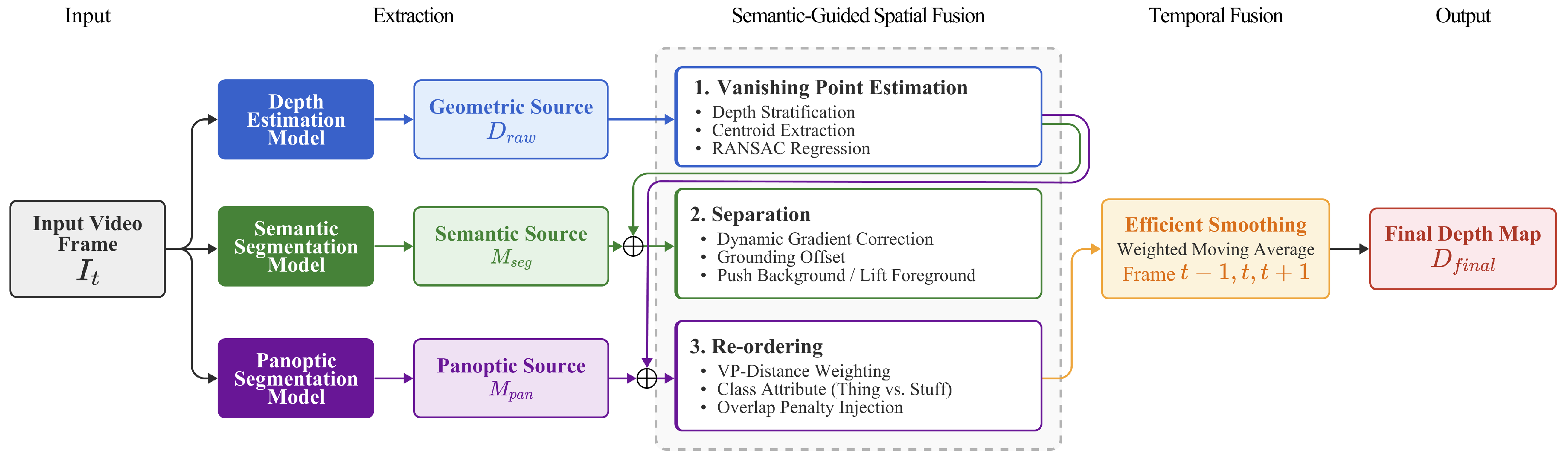
The proposed STF-Depth is a modular post-processing framework designed to maximize the performance of monocular depth estimation in video sequences. As illustrated in Figure 3, the system initiates by performing parallel extraction of complementary heterogeneous information from a single input RGB video frame I t . Leveraging three pre-trained models, the framework generates an Initial Depth Map ( D r a w ) representing geometric structures, a Semantic Segmentation Map ( M s e g ) defining regional semantics, and a Panoptic Segmentation Map ( M p a n ) identifying individual object instances. While D r a w provides global distance information but suffers from boundary degradation in texture-less regions, M s e g and M p a n lack depth data but offer precise object boundaries and instance identification cues, thereby compensating for geometric ambiguities.
These extracted inputs are refined through a sequential fusion pipeline. In the first stage, Spatial Fusion, the system robustly estimates the Vanishing Point (VP) by analyzing the statistical properties of the initial depth map and performs Dynamic Depth Gradient Correction based on this VP to physically separate background and foreground layers. Furthermore, it maximizes spatial accuracy by re-ordering the depth sequence of objects, integrating panoptic information with the distance to the vanishing point. In the subsequent Temporal Fusion stage, efficient smoothing is applied to the spatially refined frame sequence to suppress visual flickering. Through this multi-stage process, STF-Depth generates a high-quality depth map D f i n a l that is both geometrically precise and temporally stable, without requiring any additional retraining.

3.1. Heterogeneous Information Extraction

The initial stage of the proposed framework involves the parallel extraction of heterogeneous information types with complementary characteristics from a single input video frame I t . Adhering to a model-agnostic design, our system can employ any pre-trained state-of-the-art (SOTA) monocular depth estimation model as a backbone to capture the 3D geometric structure of the scene. This depth estimator analyzes texture gradients and perspective cues within the input image to generate a pixel-wise relative inverse depth map, denoted as D r a w t . While D r a w t excels at inferring the global distance hierarchy on the 2D image plane, it inherently suffers from “depth bleeding” artifacts—where object boundaries collapse in regions with uniform textures or complex lighting. In this study, D r a w t is defined as the “Raw Geometric Source,” serving as the fundamental baseline for the subsequent fusion process.
To structurally control these geometric uncertainties, the framework secures additional semantic cues independent of depth information. A general semantic segmentation model is applied first to generate a semantic segmentation map M s e g t , which performs binary classification of pixels into foreground and background. Although M s e g t does not contain distance information, it explicitly defines object boundaries. This map serves as an essential Spatial Mask in subsequent stages, particularly for distinguishing between background regions requiring Dynamic Depth Gradient Correction and object regions that must be preserved.
Furthermore, to determine precise occlusion relationships, we utilize a panoptic segmentation model in parallel. Since semantic segmentation is insufficient for separating overlapping objects or analyzing detailed object attributes, we use the panoptic model to extract not only the instance map M p a n t but also metadata including Class Labels and Confidence Scores for each instance. Crucially, the attribute distinction between countable “Things” (e.g., cars, pedestrians) and amorphous “Stuff” (e.g., sky, walls) functions as a decisive structural prior. This information directs the adaptive offset strategy in the subsequent re-ordering phase, determining whether to geometrically “pull” or “push” specific depth layers.

3.2. Semantic-Guided Spatial Fusion

The initial depth map ( D r a w ) provides continuous pixel-wise distance information but suffers from geometric ambiguities, such as the blending of foreground and background or unclear occlusion relationships. To address these issues, we propose a three-step spatial fusion algorithm that combines the statistical properties of the depth map with external semantic information.

3.2.1. Depth-Stratified and RANSAC-Based Vanishing Point Estimation

A prerequisite for accurate spatial correction is identifying the Vanishing Point (VP), the geometric center of the scene. Unlike previous approaches that often rely on Hough transforms or require prior camera calibration parameters, we propose an automatic estimation technique called Depth-Stratified Analysis, which exploits the intrinsic geometric properties of the depth map itself without any external priors.
  • Quantization: The initial depth map values are normalized and divided into N uniform depth layers. This effectively discretizes the continuous depth space into multiple analyzeable cross-sections.
  • Centroid Extraction: For each depth layer, we generate a pixel mask and calculate image moments to determine the spatial centroid C k , which represents the center of density for that layer.
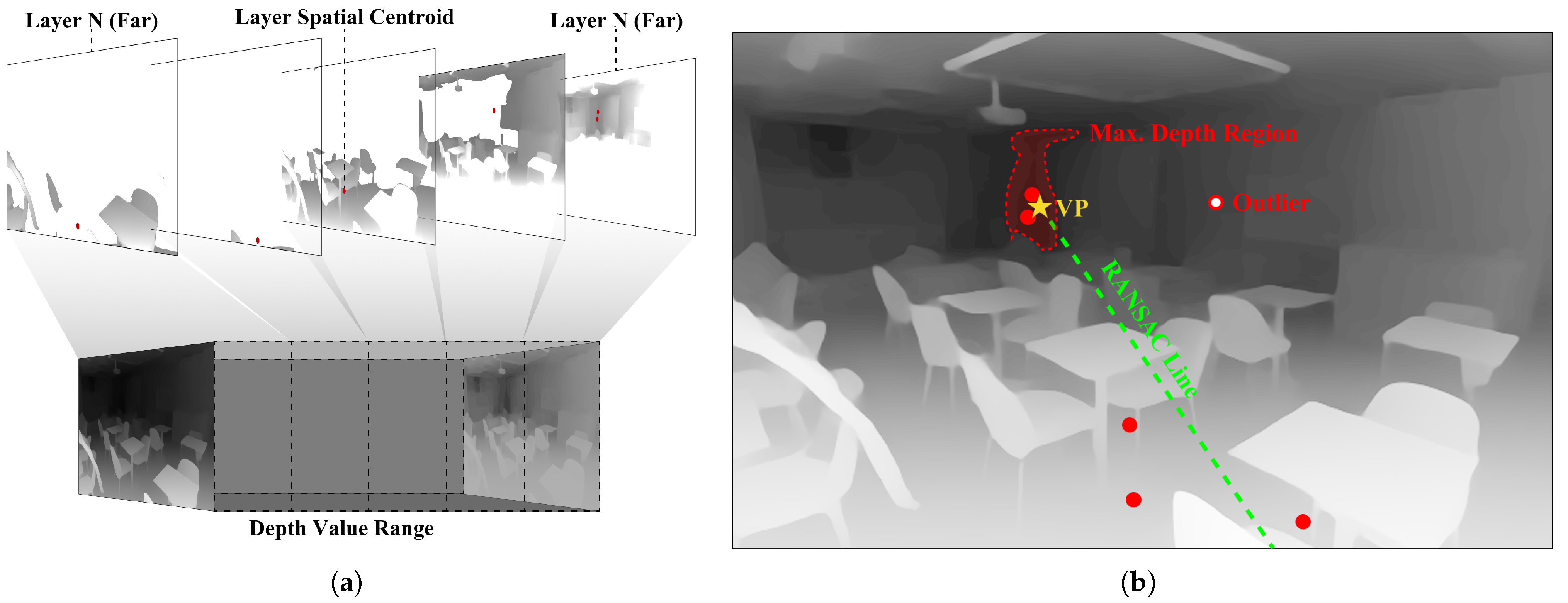
  • RANSAC Regression: Due to imperfections in the initial depth map or complex object arrangements, spatial centroids of certain layers may deviate from the main perspective trajectory. To address this, we apply the RANSAC algorithm to the set of extracted centroids C and the representative coordinate of the Max. Depth Region, denoted as P d e e p . RANSAC effectively filters out outliers—such as dynamic objects or clutter that do not align with the global perspective—and derives an optimal trend line that represents the dominant geometric structure of the scene.
    θ * = arg max m , b p P | m x p y p + b | m 2 + 1 < ϵ
    This RANSAC-based approach ensures robustness against noise, allowing for stable VP estimation even in unstructured settings where geometric cues might be partially obscured.
  • Vanishing Point Determination: The final Vanishing Point V P is defined as the point on the derived optimal trend line L θ * that minimizes the Euclidean distance to P d e e p . Here, to ensure robustness against local depth artifacts (e.g., sensor noise or reflections), P d e e p is calculated as the spatial centroid of the top 5% of pixels with the largest depth values (i.e., the Max. Depth Region visualized in Figure 4), rather than relying on a single maximum point.
    V P = arg min v L θ * v P d e e p 2

3.2.2. Foreground Separation via Dynamic Gradient Correction

Based on the estimated VP, we physically separate the depth layers of the background and foreground. Monocular depth estimation models often merge foreground and background into a single plane in regions with similar textures. To resolve this, we perform Dynamic Depth Gradient Correction reflecting the global distribution characteristics of the depth map.
First, we calculate the depth gap between the minimum ( d m i n ) and maximum ( d m a x ) values of the depth map and dynamically derive the slope a and intercept b of the correction equation, weighted by the presence of the VP. Then, using the semantic segmentation map M s e g as a mask, we apply a linear correction specifically to Foreground regions, distinct from the background.
D s e p ( p ) = D r a w ( p ) + ( a · D r a w ( p ) + b ) · I ( p Foreground )
This process performs a foundational layer separation by rescaling the depth values of foreground objects proportional to the overall depth range, ensuring they secure an independent depth volume without blending into the background.

3.2.3. Instance & VP-Distance Aware Re-Ordering

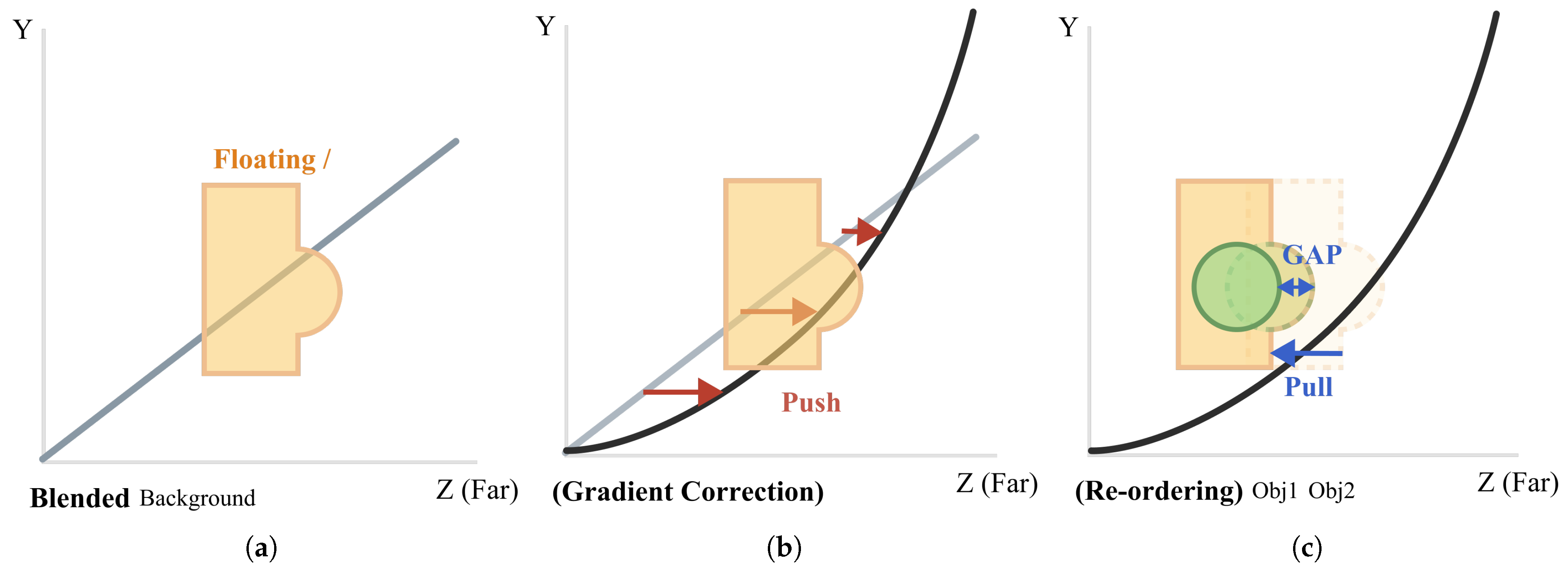
Going beyond simple separation, we perform an advanced enhancement step that simultaneously considers panoptic metadata and geometric spatial information to establish precise occlusion relationships. Figure 5 conceptually illustrates this ’Push-Pull’ strategy. This stage consists of three key mechanisms:
  • VP-Distance Weighting: According to linear perspective, depth perception sensitivity varies between the area around the VP and the periphery. We calculate the Euclidean distance d i s t ( k , V P ) between the center of each instance k and the VP. We generate a distance-proportional offset that assigns a larger weight based on the distance from the VP, performing stereoscopic correction according to the position within the frame.
  • Class Attribute Adaptation (Push-Pull Strategy): We analyze panoptic labels to distinguish whether an instance is a “Thing” (countable object, e.g., person, car) or “Stuff” (amorphous background element, e.g., sky, wall). We adopt a Dual Strategy: for “Stuff,” the calculated offset is multiplied by a negative value (−1) to push the depth layer backward, while for “Things,” a positive offset is maintained to pull it forward.
  • Overlap-based Penalty Injection: We detect spatial overlaps by analyzing the bounding boxes of instances. For overlapping pairs, we confirm the front-to-back relationship by comparing mean depths and inject an additional penalty into the overlapping region. This penalty is calculated by applying an amplification factor (1.5) to the depth difference Δ d between the two objects.
    D e n h ( p ) = D e n h ( p ) + Δ d · 1.5 ,   p ( R e g i o n f r o n t R e g i o n r e a r )
This multidimensional re-ordering process sharpens object boundaries and physically clarifies the front-to-back relationships of overlapping objects.

3.3. Efficient Temporal Fusion

Although the geometric structure and object boundaries of the depth maps have been significantly improved through the preceding spatial fusion steps, temporal inconsistencies—specifically, flickering artifacts—remain due to the independent processing of each frame. While existing video depth estimation studies have employed Optical Flow or Recurrent Neural Networks (RNNs) to track pixel-wise motion, these methods incur prohibitive computational costs, hindering real-time performance. To secure practical stability while maintaining the lightweight architecture of STF-Depth, we propose a window-based Weighted Moving Average strategy.
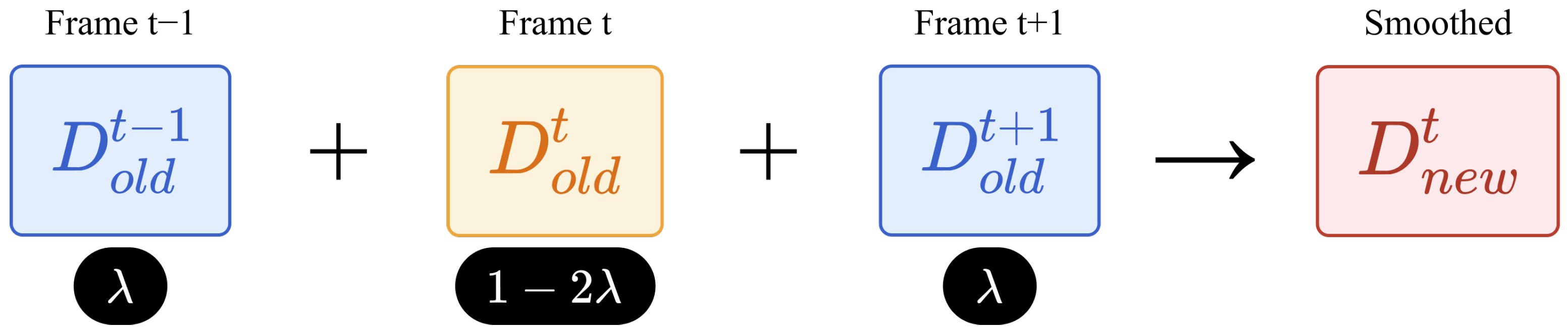
Our temporal fusion algorithm suppresses high-frequency noise by blending information from the adjacent past ( t 1 ) and future ( t + 1 ) frames, while centering on the depth information of the current frame t. The depth map D t ( k ) at the k-th iteration is updated as follows:
D t ( k ) = ( 1 2 λ ) D t ( k 1 ) + λ ( D t 1 ( k 1 ) + D t + 1 ( k 1 ) )
Here, λ denotes the temporal smoothing coefficient. In this study, we determined the optimal value of λ = 0.1 through sensitivity analysis, achieving the best trade-off between effective flickering suppression and the minimization of motion artifacts such as ghosting. Furthermore, by repeating this process for 2 iterations, we achieved an optimal balance that smooths out abrupt depth fluctuations while maximizing stability. This approach operates with a low complexity of O ( N ) , significantly reducing visual fatigue in video sequences without imposing additional computational burdens. As demonstrated in Figure 6, this method effectively smooths out high-frequency depth fluctuations, providing a stable and coherent output.

4. Experiments

4.1. Experimental Setup

4.1.1. Datasets

To verify the robust performance and generalization capability of the proposed framework across diverse imaging environments, we employed three representative datasets with distinct geometric characteristics: NYU Depth V2, KITTI, and TartanAir.
First, we utilized the NYU Depth V2 dataset for indoor environment evaluation [25]. This dataset consists of 464 diverse indoor scenes (e.g., bedrooms, offices, basements) captured using a Microsoft Kinect. Indoor scenes typically feature complex arrangements of furniture and clutter with short-range depths, making the handling of occlusions and precise boundary delineation critical. We used this dataset to focus our analysis on the instance re-ordering and spatial refinement capabilities of STF-Depth in cluttered settings.
Second, we used the KITTI dataset for outdoor environment evaluation [26]. This dataset comprises road driving sequences collected in autonomous driving scenarios, providing sparse depth information acquired via LiDAR sensors as Ground Truth. The KITTI dataset features distinct geometric structures with clear separations between the sky and road, along with numerous dynamic objects such as vehicles and pedestrians. Thus, it provides an optimal environment for validating the proposed vanishing-point-based background-foreground separation algorithm and temporal consistency in structured road scenes.
Third, to address the reviewer’s concern regarding performance in non-road or weak-perspective settings, we incorporated the TartanAir dataset [27]. Unlike KITTI, which is limited to planar motion on roads, TartanAir is a large-scale photorealistic virtual dataset collected via simulated drone flights. It features unstructured environments (e.g., abandoned factories, Japanese alleys, fantasy scenes) and aggressive 6-DoF camera motions. We selected this dataset to challenge our framework in multi-scale environments where linear perspective cues are irregular or unstable, thereby verifying the robustness of our VP estimation and temporal fusion strategies under complex geometric conditions.

4.1.2. Evaluation Metrics

To objectively validate the performance of the proposed framework, we adopted standard quantitative metrics widely established in the monocular depth estimation literature [1]. Specifically, we utilized Absolute Relative Error (AbsRel), Squared Relative Error (SqRel), Root Mean Squared Error (RMSE), Root Mean Squared Logarithmic Error ( RMSE l o g ), and Threshold Accuracy ( δ < 1.25 k for k = 1 , 2 , 3 ).
In addition to static accuracy, evaluating temporal stability is crucial for video sequences. We measured the Mean Absolute Similarity (MAS) to quantify the consistency of depth predictions between adjacent frames. For all error metrics (AbsRel, SqRel, RMSE, RMSE l o g , and MAS), lower values indicate better performance, whereas for the accuracy metrics ( δ k ), higher values denote superior performance. Detailed mathematical definitions of these standard metrics are omitted here for brevity and can be found in [1,2].

4.1.3. Implementation Details

The hardware and software specifications used for implementing the proposed framework are summarized in Table 2. The system was implemented in a Python 3.11 environment using the PyTorch 2.8.0 library, and all experiments were conducted on a workstation equipped with eight NVIDIA V100 GPUs.
We employed pre-trained SOTA models as backbones for heterogeneous information extraction. For depth estimation, we utilized MiDaS (DPT-Large), Depth Anything V2, Marigold, and ZoeDepth to validate the generalizability of our framework across different architectures [11,28,29,30,31]. For semantic segmentation, we used DeepLabV3 (ResNet-101 backbone) [13], and for panoptic segmentation, OneFormer (Swin-Large backbone) was employed [15,32]. The RANSAC algorithm for vanishing point estimation was implemented using the scikit-learn library [33].
Key hyperparameters for the Spatial Fusion stage were determined empirically. For Dynamic Depth Gradient Correction, the slope coefficients were adaptively set to 0.1 or 0.05 depending on the presence of a vanishing point. For Instance Re-ordering, the instance confidence threshold was set to 0.7 to exclude uncertain predictions, and the overlap penalty amplification factor was set to 1.5. In the Temporal Fusion stage, we applied a smoothing factor of λ = 0.1 with 2 iterations for the weighted moving average. This configuration effectively suppressed temporal flickering while minimizing motion artifacts such as ghosting.

4.2. Ablation Study

The proposed framework is designed to maximize depth estimation performance by sequentially integrating geometric, semantic, and temporal information. In this section, we conduct an ablation study to isolate and quantify the individual contribution of each core module to the overall performance improvement, thereby validating the rationale behind our fusion pipeline design. To achieve this, we structured the experiment into four progressive cases, incrementally adding each function to the baseline model.
  • Method A (Baseline): The original output of the pre-trained monocular depth estimation model without any post-processing ( D r a w ).
  • Method B (+ Separation): Baseline with the Background-Foreground Depth Separation (Section 3.2.2) module applied. This stage corrects background perspective and eliminates floating artifacts using semantic masks and vanishing point estimation.
  • Method C (+ Re-ordering): Method B with the addition of the Instance-Aware Depth Re-ordering (Section 3.2.3) module. This stage rearranges the depth order of overlapping objects and injects separation margins using panoptic information.
  • Method D (Full STF-Depth): The final framework integrating the Efficient Temporal Fusion (Section 3.3) module into Method C.
Through this stepwise evaluation, we demonstrate how the logical fusion of heterogeneous information sources—rather than a mere combination of models—synergistically reduces errors (RMSE, AbsRel) and enhances visual completeness.

4.2.1. Baseline Only

Table 3 presents the initial performance of the baseline models without any post-processing. The results indicate that metric depth-based models, such as Marigold and ZoeDepth, demonstrated respectable initial performance with relatively low AbsRel and RMSE errors. In contrast, relative depth models like MiDaS and Depth Anything V2 exhibited higher error rates and lower accuracy ( δ 1 ). This discrepancy is largely attributed to the inherent scale ambiguity of monocular depth estimation, where the global scale of the predicted depth map does not align with the metric ground truth. These baseline metrics serve as the reference point for evaluating the incremental contributions of the proposed STF-Depth modules.

4.2.2. Baseline + Spatial Fusion

Table 4 summarizes the performance changes after applying the Background-Foreground Depth Separation module. The results show a significant improvement in geometric accuracy across most backbone models. Notably, Depth Anything V2 and MiDaS exhibited the largest performance gains, with substantial reductions in AbsRel and RMSE. This confirms that our RANSAC-based Vanishing Point Estimation and Dynamic Depth Gradient Correction effectively rectify perspective distortions in texture-less background regions and calibrate the global scale of the depth map closer to the metric ground truth. Thus, the spatial fusion stage plays a decisive role in bridging the gap between relative and absolute depth.

4.2.3. Baseline + Spatial + Re-Ordering Fusion

Table 5 illustrates the results after incorporating the Instance-Aware Depth Re-ordering module. In this stage, global error metrics such as RMSE tended to remain similar to Model B or showed marginal fluctuations. This is attributed to the artificial adjustment of pixel-wise depth values during the injection of Separation Margins between overlapping objects using panoptic metadata. Although the numerical error reduction is modest, this process clarifies occlusion relationships and sharply recovers ambiguous boundaries, making it an essential step for enhancing structural integrity that is not fully captured by quantitative metrics alone.

4.2.4. Baseline + Spatial + Re-Ordering + Temporal Fusion (Full STF-Depth)

Table 6 displays the performance of the complete proposed framework, which integrates Efficient Temporal Fusion. The evaluation metrics based on static images (e.g., AbsRel) remain comparable to the previous stage (Model C), indicating that temporal smoothing was applied without compromising the geometric structure of individual frames. However, from a video sequence perspective, this module plays a critical role in ensuring temporal consistency by suppressing high-frequency flickering. In conclusion, STF-Depth demonstrates consistent performance improvement and stability across various backbone models, including Depth Anything V2, Marigold, and MiDaS, confirming its versatility as a robust, model-agnostic framework.

4.3. Quantitative Results

Following the ablation study, which internally validated the contribution of each module within our proposed framework, this section conducts comparative experiments with state-of-the-art (SOTA) monocular depth estimation models to demonstrate the generalized utility and performance superiority of STF-Depth. We selected widely adopted models as baselines, including MiDaS v3.1 trained on large-scale mixed datasets, the Transformer-based DPT (Dense Prediction Transformer), and GLPDepth, which considers both global and local contexts [34].
We aim to prove that STF-Depth functions as a plug-and-play module capable of consistently enhancing the performance of various backbone models, rather than being limited to a specific architecture. To this end, we directly compare the original outputs of each SOTA model (Baseline) against the results obtained after applying STF-Depth (Ours) on the same datasets. The evaluation is conducted from two primary perspectives: Section 4.3.1 analyzes the physical accuracy of depth estimation using the full set of standard metrics (AbsRel, SqRel, RMSE, RMSE l o g , and δ ) against Ground Truth from the NYU Depth V2 and KITTI datasets, while Section 4.3.2 quantitatively assesses the temporal consistency by measuring frame-to-frame variations in video sequences.

4.3.1. Depth Estimation Quality Analysis

Table 7 compares the performance of four SOTA backbone models before and after applying STF-Depth on the NYU Depth V2, KITTI and TartanAir datasets. The results reveal distinct performance improvement patterns depending on the training paradigm of the base models.
First, the most significant improvements were observed in relative depth estimation models such as Depth Anything V2 and MiDaS v3.1. While these models initially exhibited high error rates due to scale discrepancies with the ground truth, applying STF-Depth resulted in substantial improvements in geometric accuracy. Notably, for MiDaS v3.1, applying STF-Depth resulted in a significant reduction of AbsRel by approximately 25.7% and an improvement in RMSE by 51.6% on the KITTI dataset. This suggests that our RANSAC-based Vanishing Point Estimation and Dynamic Depth Gradient Correction successfully calibrated the global scale of the depth maps closer to the physical ground truth.
Conversely, for models trained to predict metric depth directly, such as Marigold and ZoeDepth, the numerical performance remained stable or showed slight fluctuations. This is attributed to a trade-off where STF-Depth prioritizes Qualitative Quality—injecting separation margins between objects—which may result in the smoothing of fine-grained pixel-wise depth values (Metric Precision). Nevertheless, the δ < 1.25 accuracy metric remained stable even in these cases, demonstrating that our framework enhances geometric structure without compromising the inference capabilities of the original models.

4.3.2. Temporal Consistency Analysis

Quantitative metrics based on single images are insufficient for evaluating temporal stability, a critical aspect of video depth estimation. Therefore, we quantified temporal consistency using the Mean Absolute Similarity (MAS) metric, which measures the variation in depth values between adjacent frames.
Experimental results indicate that baseline models recorded a high MAS value of 4.578 due to flickering artifacts—subtle fluctuations in depth values even in static backgrounds—caused by independent per-frame processing. In contrast, STF-Depth effectively suppressed such high-frequency noise through the Efficient Temporal Fusion module. Consequently, as shown in Table 8, the MAS value for STF-Depth decreased to 3.401, representing a significant reduction in volatility of approximately 25.70% compared to the baseline.
This improvement is particularly significant given that it was achieved without complex computational processes [24,35]. Generally, state-of-the-art models in video depth estimation (e.g., STATIC [36], MAMo), which utilize Optical Flow Warping to align temporal consistency, report metric improvements (e.g., rTC, aTC) in the range of 20–30%. While some aggressive methods (e.g., FutureDepth [37]) achieve up to 48% improvement, our study achieved a competitive 25.70% gain solely through a weighted moving average, without the high-cost warping operations involved in calculating motion vector fields F t t + 1 and re-projecting pixels D ^ t + 1 ( p ) = D t ( p + F ( p ) ) . This numerically proves that STF-Depth achieves an optimal trade-off between computational efficiency and temporal stability.

4.4. Qualitative Results

To evaluate perceptual quality and geometric integrity beyond quantitative error rates, we conducted a qualitative comparison using the NYU Depth V2, KITTI, and TartanAir datasets, representing complex indoor, structured outdoor, and unstructured virtual environments, respectively.
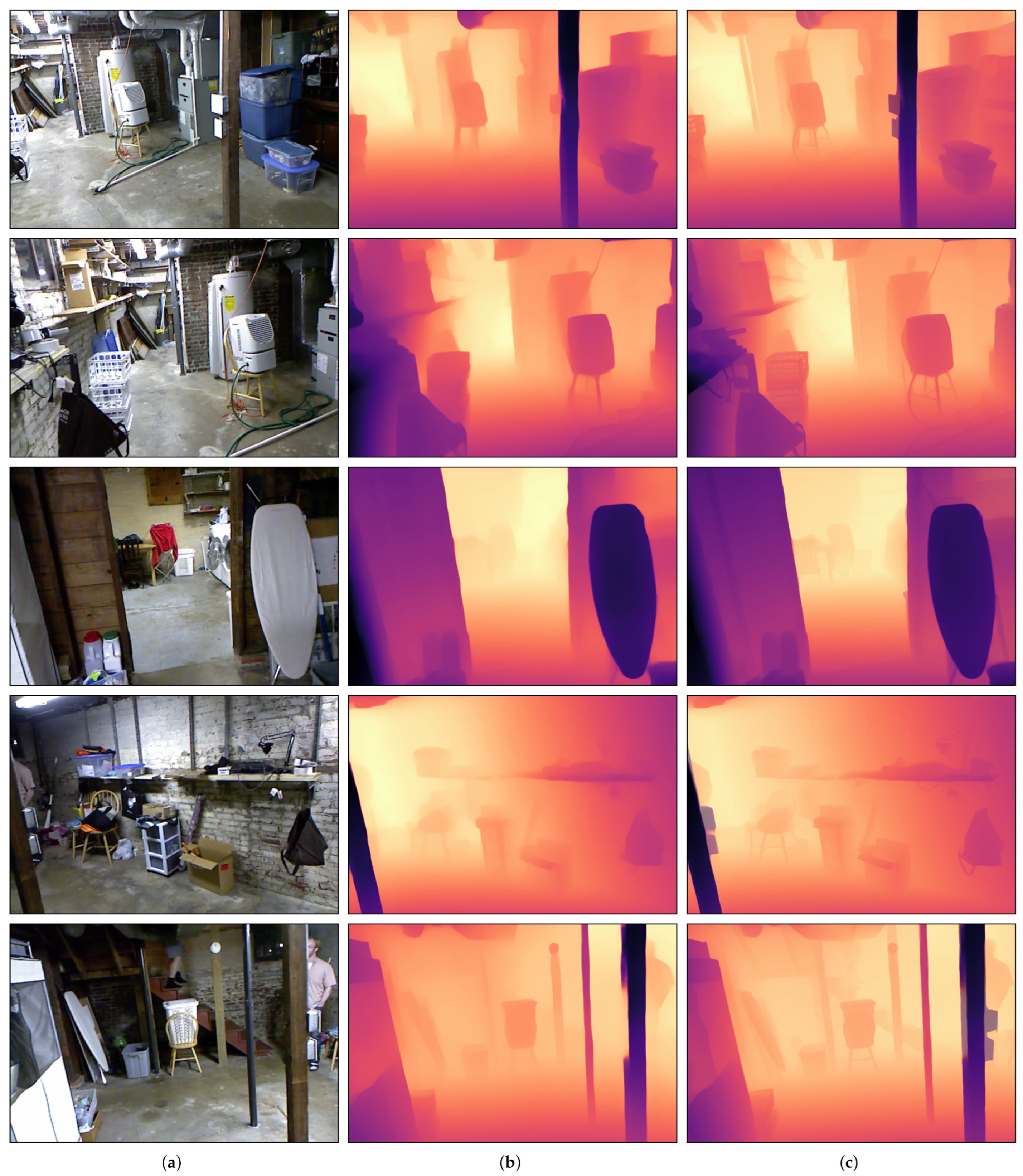
First, Figure 7 illustrates the qualitative comparison results for the indoor environment using NYU Depth V2. The baseline MiDaS frequently exhibited boundary blurring or merged foreground objects with background walls, particularly in cluttered scenes containing desks, chairs, and sofas. In contrast, STF-Depth successfully ”popped out” overlapping objects by applying Instance-Aware Re-ordering, establishing clear depth ordering. Notably, it sharply recovered fine structural details, such as furniture legs and edges, thereby enhancing visual clarity.
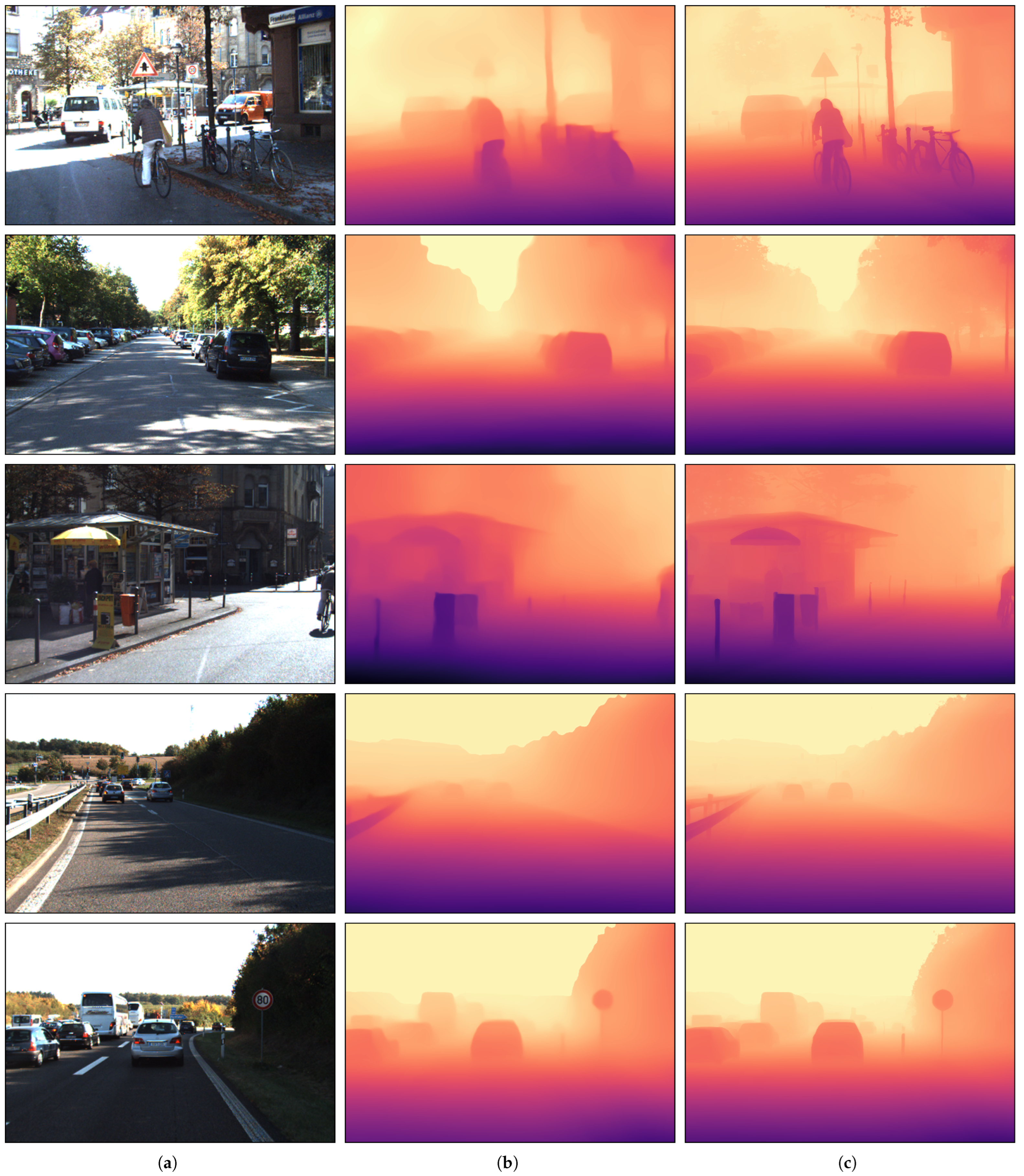
Second, the evaluation results for the outdoor environment using KITTI are presented in Figure 8. In these scenarios, the primary challenge lay in separating vehicles and pedestrians from the road and sky. The baseline model tended to produce flattened depth perceptions or distorted perspectives in texture-less road regions. Conversely, STF-Depth significantly enhanced global stereoscopy through Vanishing Point-based Dynamic Gradient Correction. By naturally “pushing” the background (road and sky) toward the vanishing point and “pulling” foreground objects (vehicles) forward, our method achieved a more physically plausible depth representation with stable grounding.
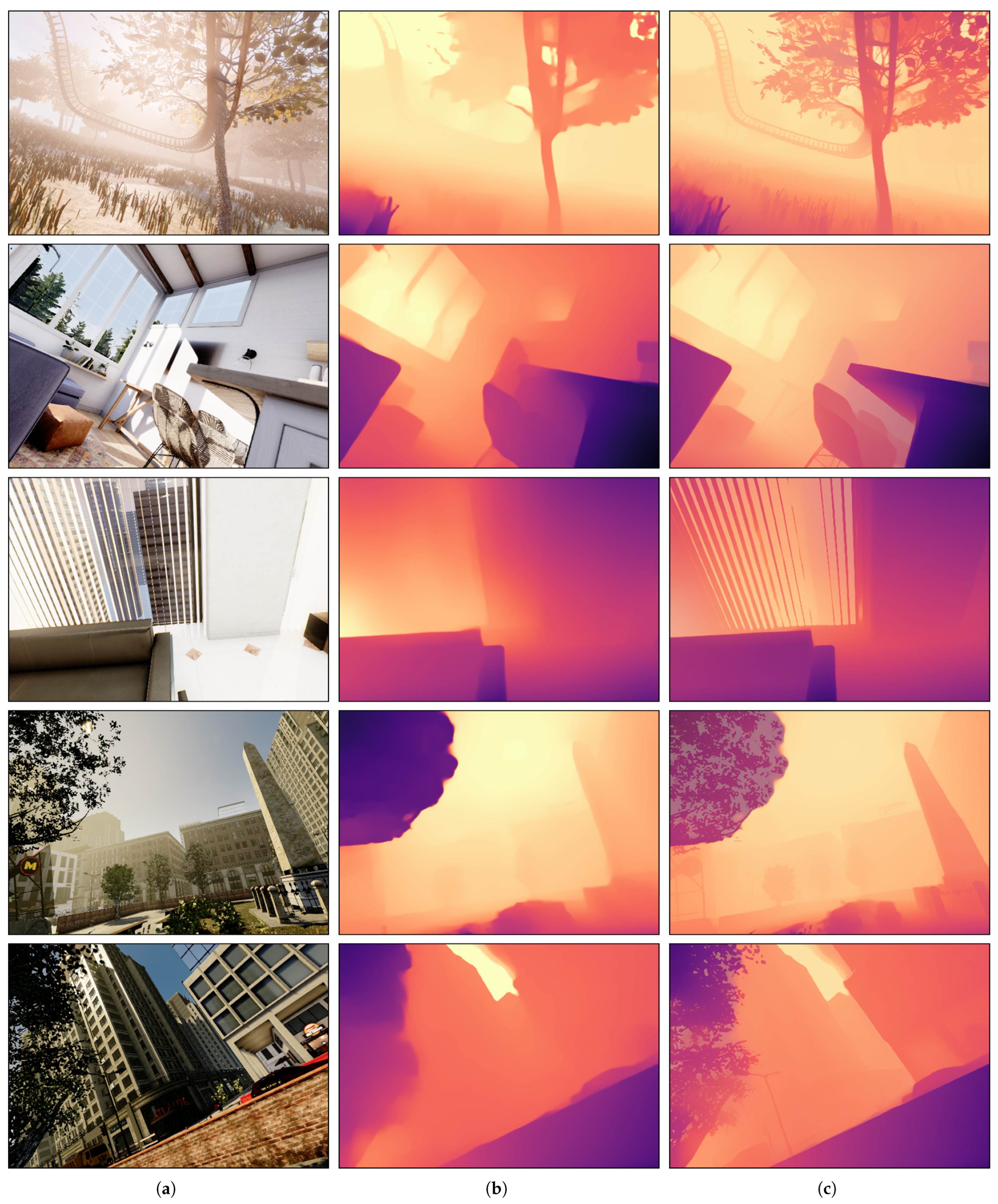
Third, Figure 9 demonstrates the evaluation results in unstructured environments using the TartanAir dataset. Unlike road-centric KITTI scenes, TartanAir features aggressive 6-DoF camera motions and irregular geometries. While the baseline model often struggles with perspective distortion due to the lack of standard road cues, STF-Depth effectively stabilizes the global structure. By leveraging depth-stratified VP estimation, our method robustly separates scene layers, proving its generalization capability even in non-standard navigation scenarios.

5. Discussion

5.1. Analysis of Performance Improvements and Theoretical Implications

The experimental results of this study suggest that fusing heterogeneous information is a highly effective strategy for resolving the inherent geometric ambiguities of Monocular Depth Estimation (MDE). The significant reduction in RMSE and AbsRel observed in the quantitative evaluation stems from the successful reconstruction of the depth map’s physical structure by the Spatial Fusion module of STF-Depth.
In particular, the RANSAC-based Vanishing Point Estimation and Dynamic Depth Gradient Correction played a decisive role in linearly correcting depth distortions in texture-less background regions, thereby calibrating the global scale of the depth map to resemble the real world more closely. Furthermore, Instance Re-ordering utilizing panoptic metadata (Thing vs. Stuff) and distance to the vanishing point enabled adaptive processing—pulling or pushing depth layers based on intrinsic object attributes—going beyond simple planar separation to drastically improve boundary sharpness and stereoscopy. This demonstrates that performance can be significantly enhanced simply by injecting geometric and semantic “constraints” as post-processing into the “inferred depth” generated by deep learning models.
In terms of temporal aspects, this study demonstrates the efficiency of achieving stability without Optical Flow. Existing approaches, such as Neural Video Depth Stabilizer or FutureDepth, resolve temporal inconsistencies by tracking pixel motion vectors between frames and performing Warping to re-project previous depth values onto the current coordinate system. While precise, this method incurs high computational costs. In contrast, STF-Depth adopts a low-pass filter approach that selectively removes high-frequency flickering, based on the assumption that the geometric structure between adjacent video frames does not change abruptly. The observed 25.70% improvement in consistency suggests that simple time-series smoothing is sufficiently effective for practical video stabilization, even without complex motion compensation.

5.2. Limitations

Despite its superior performance and versatility, the proposed framework has structural limitations inherent to its pipeline design.

5.2.1. Dependency on Pre-Processing Models

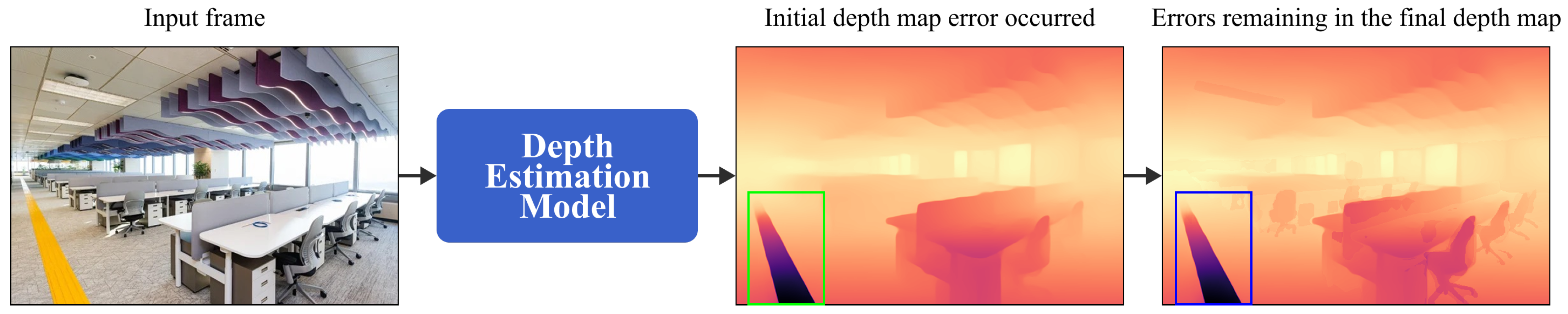
Proposed method operates on the assumption that the results from semantic segmentation, panoptic segmentation, and the initial depth estimation model are reliable sources of information. Consequently, the final performance of STF-Depth is heavily dependent on the accuracy of these pre-processing models. When rare textures or complex patterns not present in the training data appear, there is a risk that the initial models may fail to interpret them correctly. As shown in Figure 10, in an indoor office environment, if the initial depth estimation model fails to correctly recognize the geometric structure of specific patterns, such as tactile paving (braille blocks) on the floor, and generates depth errors, the proposed fusion pipeline faces limitations in distinguishing these from background noise for correction. Consequently, the geometric defects from the initial stage are not rectified and persist in the final depth map.

5.2.2. Real-Time Processing Constraints and Efficiency Analysis

Although STF-Depth offers the significant advantage of requiring no retraining, it faces computational challenges during inference, as it necessitates the execution of three high-performance deep learning models: monocular depth estimation, semantic segmentation, and panoptic segmentation. In our efficiency benchmark conducted on an NVIDIA Tesla V100 GPU (NVIDIA Corporation, Santa Clara, CA, USA), the baseline model (MiDaS only) demonstrated real-time capability with an average inference time of 100.10 ms (approx. 9.99 FPS)and a peak GPU memory usage of 2.57 GB.
In contrast, when running the full STF-Depth framework, the per-frame processing time increased to 825.15 ms (approx. 1.21 FPS), and peak memory consumption rose to 3.53 GB, as summarized in Table 9. This increase is attributed to the cumulative computational load of heavy backbones such as DPT-Large and Swin-Large. While the current performance is sufficient for offline video processing, it presents limitations for ensuring online stream processing on resource-constrained platforms like autonomous driving systems or mobile edge devices, where ultra-low latency is critical. This highlights the necessity for future work to optimize the model and accelerate inference speed through the proposed “Single ViT-based Unified Architecture.”

5.2.3. Single Vanishing Point and Linear Perspective Assumptions

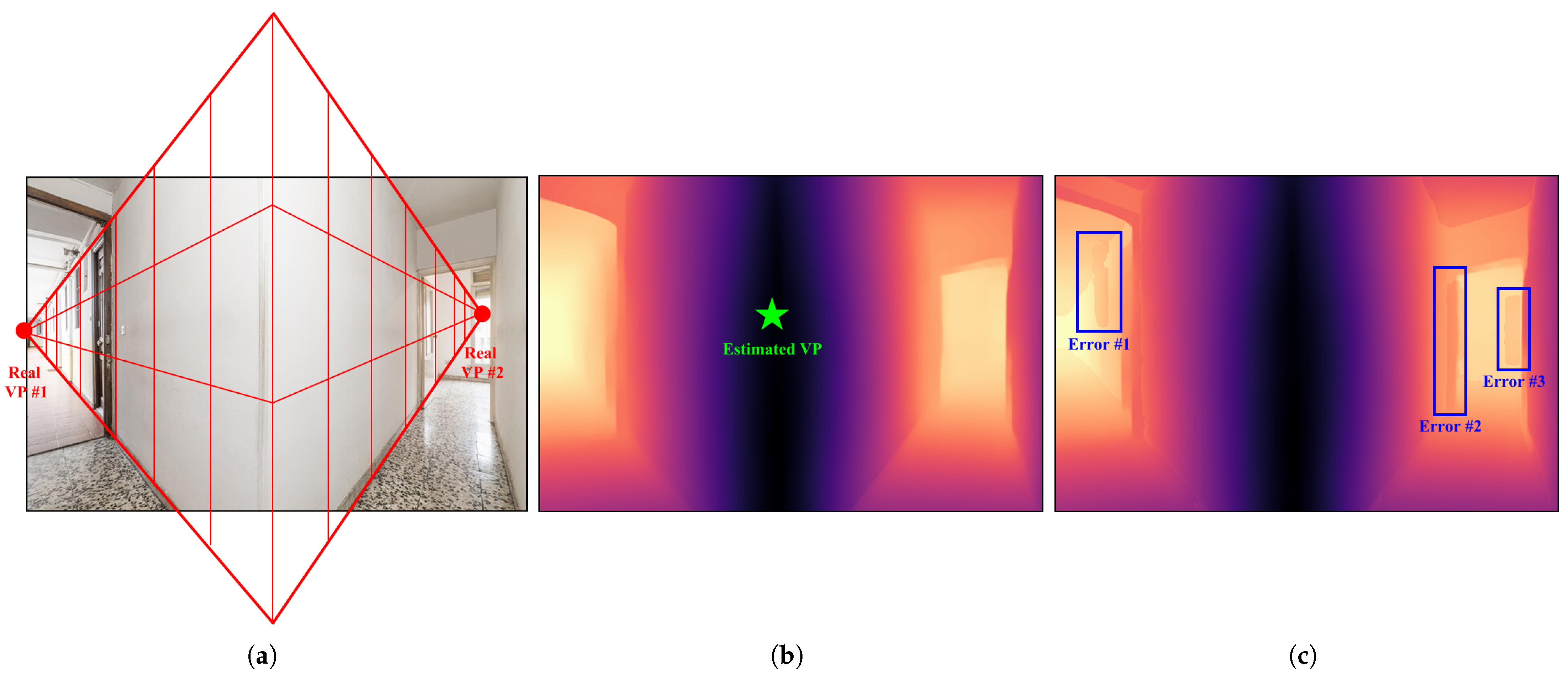
The vanishing point estimation algorithm in this study operates under the premise that geometric elements within the scene converge to a single dominant vanishing point. Specifically, the RANSAC-based approach performs optimally in structured environments exhibiting strong linear perspective, such as straight highways, corridors, or tunnels. However, as shown in Figure 8 and Figure 11, limitations may arise in complex scenarios where multiple vanishing points exist—such as curved roads, intersections, or urban environments with diverse building orientations—or in weak perspective settings (e.g., cluttered indoor scenes with irregular furniture arrangements). In such unstructured environments, the algorithm might overfit to a specific vanishing point or misestimate the geometric center. Consequently, this can lead to inaccurate depth gradient corrections during the application of the “Push-Pull” strategy. Future work should therefore focus on extending the framework to detect multiple vanishing points or handle non-linear geometric structures adaptively.

5.3. Future Work

To overcome the limitations of the current post-processing pipeline and fundamentally innovate system efficiency and learning capability, future research will explore two main directions.
First, we aim to develop a Single ViT-based Unified Multi-Task Architecture. The current framework incurs significant computational redundancy by independently running three separate backbone models for depth estimation, semantic segmentation, and panoptic segmentation. To address this, we plan to design a unified network where a single shared ViT (Vision Transformer) Encoder extracts global features, which are then processed by Multi-Head Decoders dedicated to depth, semantic, and instance tasks, respectively. This architecture will not only secure real-time performance by reducing encoder operations to a single pass but also maximize fusion synergy by encouraging the mutually complementary learning of geometric and semantic information within the latent space.
Second, we intend to transition toward End-to-End Fusion Learning. We plan to replace the current heuristic-based algorithms (e.g., RANSAC, offset correction) with differentiable neural network modules. This will allow the entire process—from input video to the final refined depth map—to be trained within a single network. Through this approach, we aim to learn fusion weights directly from data that are robust to pre-processing errors, ultimately completing a sophisticated depth estimation model capable of adaptive operation even in complex video environments.

6. Conclusions

In this paper, we proposed STF-Depth, a novel post-processing framework designed to enhance the geometric accuracy and temporal consistency of Monocular Depth Estimation (MDE) models without the need for additional retraining. By logically fusing heterogeneous information—including depth-stratified vanishing point estimation, semantic-guided spatial refinement, and instance-aware re-ordering—our approach effectively resolves common artifacts such as scale ambiguity, boundary blurring, and temporal flickering.
Extensive experimental evaluations on the NYU Depth V2, KITTI, and TartanAir datasets demonstrated that STF-Depth generalizes robustly across diverse environments, ranging from structured indoor scenes to complex outdoor and unstructured virtual settings. Notably, our framework achieved a 25.7% reduction in Absolute Relative error (AbsRel) on the NYU Depth V2 dataset and showed significant improvements in temporal stability compared to state-of-the-art backbone models. These results confirm that STF-Depth serves as a practical, universal plug-and-play module capable of upgrading existing MDE models for high-precision applications.
Despite these achievements, the current multi-stage pipeline relying on separate heavy backbone networks limits real-time processing capabilities. In future work, we aim to address this efficiency bottleneck by distilling the proposed geometric and semantic constraints into a unified, lightweight end-to-end architecture, thereby enabling real-time inference suitable for resource-constrained platforms such as mobile robotics and autonomous drones.

Author Contributions

Conceptualization, H.K. (Hyunsu Kim), J.J. and Y.S.; methodology, H.K. (Hyunsu Kim) and Y.S.; software, H.K. (Hyunsu Kim); validation, H.K. (Hyunsu Kim), Y.L., H.K. (Hyunseong Ko) and Y.S.; formal analysis, H.K. (Hyunsu Kim), J.J. and Y.S.; investigation, H.K. (Hyunsu Kim); resources, H.K. (Hyunsu Kim); data curation, H.K. (Hyunsu Kim) and Y.L.; writing—original draft preparation, H.K. (Hyunsu Kim); writing—review and editing, H.K. (Hyunsu Kim), J.J. and Y.S.; visualization, H.K. (Hyunsu Kim), Y.L. and H.K. (Hyunseong Ko); supervision, Y.S.; project administration, Y.S.; funding acquisition, Y.S. All authors have read and agreed to the published version of the manuscript.

Funding

This study was supported by the commercialization promotion agency for R&D outcomes grant funded by the Korea government (MSIT) (2710086167). This work was supported by the Commercialization Promotion Agency for R&D Outcomes (COMPA) grant funded by the Korea government (Ministry of Science and ICT) (RS-2025-02412990). This research was supported by the MSIT (Ministry of Science and ICT), Korea, under the ITRC (Information Technology Research Center) support program (IITP-2025-2020-0-01789) supervised by the IITP (Institute for Information & Communications Technology Planning & Evaluation). This research was supported by the Regional Innovation System & Education (RISE) through the Seoul RISE Center, funded by the Ministry of Education (MOE) and the Seoul Metropolitan Government. (2025-RISE-01-007-04).

Institutional Review Board Statement

Not applicable.

Informed Consent Statement

Not applicable.

Data Availability Statement

Publicly available datasets were analyzed in this study. The NYU Depth V2 dataset is available at https://cs.nyu.edu/~silberman/datasets/nyu_depth_v2.html (accessed on 15 December 2023), the KITTI dataset is available at http://www.cvlibs.net/datasets/kitti (accessed on 15 December 2023), and the TartanAir dataset is available at https://tartanair.org (accessed on 15 December 2023). The implementation code and models proposed in this study are available at https://github.com/PLASS-Lab/STF-Depth (accessed on 15 December 2023).

Conflicts of Interest

The authors declare no conflicts of interest.

References

  1. Eigen, D.; Puhrsch, C.; Fergus, R. Depth map prediction from a single image using a multi-scale deep network. Adv. Neural Inf. Process. Syst. 2014, 27, 2366–2374. [Google Scholar]
  2. Birkl, R.; Wofk, D.; Müller, M. MiDaS v3.1—A Model Zoo for Robust Monocular Relative Depth Estimation. arXiv 2023, arXiv:2307.14460. [Google Scholar]
  3. Yang, L.; Kang, B.; Huang, Z.; Xu, X.; Feng, J.; Zhao, H. Depth Anything: Unleashing the Power of Large-Scale Unlabeled Data. arXiv 2024, arXiv:2401.10891. [Google Scholar] [CrossRef] [Scilit]
  4. Kim, H.; Son, Y. Generating Multi-View Action Data from a Monocular Camera Video by Fusing Human Mesh Recovery and 3D Scene Reconstruction. Appl. Sci. 2025, 15, 10372. [Google Scholar] [CrossRef] [Scilit]
  5. Wang, S. Development of approach to an automated acquisition of static street view images using transformer architecture for analysis of Building characteristics. Sci. Rep. 2025, 15, 29062. [Google Scholar] [CrossRef] [Scilit] [PubMed]
  6. Wang, S.; Park, S.; Kim, J.; Kim, J. Safety helmet monitoring on construction sites using YOLOv10 and advanced transformer architectures with surveillance and body-worn cameras. J. Constr. Eng. Manag. 2025, 151, 04025186. [Google Scholar] [CrossRef] [Scilit]
  7. Watson, J.; Aodha, O.M.; Prisacariu, V.; Brostow, G.; Firman, M. The Temporal Opportunist: Self-Supervised Multi-Frame Monocular Depth. arXiv 2021, arXiv:2104.14540. [Google Scholar]
  8. Chen, S.; Guo, H.; Zhu, S.; Zhang, F.; Huang, Z.; Feng, J.; Kang, B. Video Depth Anything: Consistent Depth Estimation for Super-Long Videos. arXiv 2025, arXiv:2501.12375. [Google Scholar] [CrossRef] [Scilit]
  9. Dosovitskiy, A. An image is worth 16x16 words: Transformers for image recognition at scale. arXiv 2020, arXiv:2010.11929. [Google Scholar]
  10. Ranftl, R.; Lasinger, K.; Hafner, D.; Schindler, K.; Koltun, V. Towards robust monocular depth estimation: Mixing datasets for zero-shot cross-dataset transfer. IEEE Trans. Pattern Anal. Mach. Intell. 2020, 44, 1623–1637. [Google Scholar]
  11. Ranftl, R.; Bochkovskiy, A.; Koltun, V. Vision transformers for dense prediction. In Proceedings of the IEEE/CVF International Conference on Computer Vision, Montreal, BC, Canada, 11–17 October 2021; pp. 12179–12188. [Google Scholar]
  12. Zhang, Q.; Zhu, Y.; Cordeiro, F.R.; Chen, Q. PSSCL: A progressive sample selection framework with contrastive loss designed for noisy labels. Pattern Recognit. 2025, 161, 111284. [Google Scholar] [CrossRef] [Scilit]
  13. Chen, L.C.; Papandreou, G.; Kokkinos, I.; Murphy, K.; Yuille, A.L. Deeplab: Semantic image segmentation with deep convolutional nets, atrous convolution, and fully connected crfs. IEEE Trans. Pattern Anal. Mach. Intell. 2017, 40, 834–848. [Google Scholar] [CrossRef] [Scilit] [PubMed]
  14. Kirillov, A.; He, K.; Girshick, R.; Rother, C.; Dollár, P. Panoptic segmentation. In Proceedings of the IEEE/CVF Conference on Computer Vision and Pattern Recognition, Long Beach, CA, USA, 15–20 June 2019; pp. 9404–9413. [Google Scholar]
  15. Jain, J.; Li, J.; Chiu, M.T.; Hassani, A.; Orlov, N.; Shi, H. Oneformer: One transformer to rule universal image segmentation. In Proceedings of the IEEE/CVF Conference on Computer Vision and Pattern Recognition, Vancouver, BC, Canada, 18–22 June 2023; pp. 2989–2998. [Google Scholar]
  16. Teed, Z.; Deng, J. Raft: Recurrent all-pairs field transforms for optical flow. In Proceedings of the European Conference on Computer Vision, Glasgow, UK, 23–28 August 2020; Springer: Berlin/Heidelberg, Germany, 2020; pp. 402–419. [Google Scholar]
  17. Eom, C.; Park, H.; Ham, B. Temporally consistent depth prediction with flow-guided memory units. IEEE Trans. Intell. Transp. Syst. 2019, 21, 4626–4636. [Google Scholar] [CrossRef] [Scilit]
  18. Watson, J.; Mac Aodha, O.; Prisacariu, V.; Brostow, G.; Firman, M. The temporal opportunist: Self-supervised multi-frame monocular depth. In Proceedings of the IEEE/CVF Conference on Computer Vision and Pattern Recognition, Nashville, TN, USA, 19–25 June 2021; pp. 1164–1174. [Google Scholar]
  19. Patil, V.; Van Gansbeke, W.; Dai, D.; Van Gool, L. Don’t forget the past: Recurrent depth estimation from monocular video. IEEE Robot. Autom. Lett. 2020, 5, 6813–6820. [Google Scholar] [CrossRef] [Scilit]
  20. Chen, S.; Guo, H.; Zhu, S.; Zhang, F.; Huang, Z.; Feng, J.; Kang, B. Video Depth Anything: Consistent Depth Estimation for Super-Long Videos. In Proceedings of the IEEE/CVF Conference on Computer Vision and Pattern Recognition (CVPR), Nashville, TN, USA, 11–15 June 2025; pp. 22831–22840. [Google Scholar]
  21. Luo, X.; Huang, J.B.; Szeliski, R.; Matzen, K.; Kopf, J. Consistent video depth estimation. ACM Trans. Graph. (ToG) 2020, 39, 71:1–71:13. [Google Scholar]
  22. Arnab, A.; Dehghani, M.; Heigold, G.; Sun, C.; Lučić, M.; Schmid, C. Vivit: A video vision transformer. In Proceedings of the IEEE/CVF International Conference on Computer Vision, Montreal, BC, Canada, 10–17 October 2021; pp. 6836–6846. [Google Scholar]
  23. Li, S.; Luo, Y.; Zhu, Y.; Zhao, X.; Li, Y.; Shan, Y. Enforcing temporal consistency in video depth estimation. In Proceedings of the IEEE/CVF International Conference on Computer Vision, Montreal, BC, Canada, 10–17 October 2021; pp. 1145–1154. [Google Scholar]
  24. Wang, Y.; Shi, M.; Li, J.; Huang, Z.; Cao, Z.; Zhang, J.; Xian, K.; Lin, G. Neural video depth stabilizer. In Proceedings of the IEEE/CVF International Conference on Computer Vision, Paris, France, 4–6 October 2023; pp. 9466–9476. [Google Scholar]
  25. Silberman, N.; Hoiem, D.; Kohli, P.; Fergus, R. Indoor segmentation and support inference from rgbd images. In Proceedings of the European conference on Computer Vision, Florence, Italy, 7–13 October 2012; Springer: Berlin/Heidelberg, Germany, 2012; pp. 746–760. [Google Scholar]
  26. Geiger, A.; Lenz, P.; Urtasun, R. Are we ready for autonomous driving? the kitti vision benchmark suite. In Proceedings of the 2012 IEEE Conference on Computer Vision and Pattern Recognition, Providence, RI, USA, 16–21 June 2012; IEEE: New York, NY, USA, 2012; pp. 3354–3361. [Google Scholar]
  27. Wang, W.; Zhu, D.; Wang, X.; Hu, Y.; Qiu, Y.; Wang, C.; Hu, Y.; Kapoor, A.; Scherer, S. TartanAir: A Dataset to Push the Limits of Visual SLAM. In Proceedings of the 2020 IEEE/RSJ International Conference on Intelligent Robots and Systems (IROS), Las Vegas, NV, USA, 24 October 2020–24 January 2021. [Google Scholar]
  28. Yang, L.; Kang, B.; Huang, Z.; Zhao, Z.; Xu, X.; Feng, J.; Zhao, H. Depth anything v2. Adv. Neural Inf. Process. Syst. 2024, 37, 21875–21911. [Google Scholar]
  29. Yang, L.; Kang, B.; Huang, Z.; Xu, X.; Feng, J.; Zhao, H. Depth anything: Unleashing the power of large-scale unlabeled data. In Proceedings of the IEEE/CVF Conference on Computer Vision and Pattern Recognition, Seattle, WA, USA, 16–22 June 2024; pp. 10371–10381. [Google Scholar]
  30. Ke, B.; Qu, K.; Wang, T.; Metzger, N.; Huang, S.; Li, B.; Obukhov, A.; Schindler, K. Marigold: Affordable Adaptation of Diffusion-Based Image Generators for Image Analysis. arXiv 2025, arXiv:2505.09358. [Google Scholar] [CrossRef] [Scilit] [PubMed]
  31. Bhat, S.F.; Birkl, R.; Wofk, D.; Wonka, P.; Müller, M. Zoedepth: Zero-shot transfer by combining relative and metric depth. arXiv 2023, arXiv:2302.12288. [Google Scholar]
  32. Liu, Z.; Lin, Y.; Cao, Y.; Hu, H.; Wei, Y.; Zhang, Z.; Lin, S.; Guo, B. Swin transformer: Hierarchical vision transformer using shifted windows. In Proceedings of the IEEE/CVF International Conference on Computer Vision, Montreal, BC, Canada, 10–17 October 2021; pp. 10012–10022. [Google Scholar]
  33. Fischler, M.A.; Bolles, R.C. Random sample consensus: A paradigm for model fitting with applications to image analysis and automated cartography. Commun. ACM 1981, 24, 381–395. [Google Scholar] [CrossRef] [Scilit]
  34. Kim, D.; Ka, W.; Ahn, P.; Joo, D.; Chun, S.; Kim, J. Global-local path networks for monocular depth estimation with vertical cutdepth. arXiv 2022, arXiv:2201.07436. [Google Scholar] [CrossRef] [Scilit]
  35. Lai, W.S.; Huang, J.B.; Wang, O.; Shechtman, E.; Yumer, E.; Yang, M.H. Learning blind video temporal consistency. In Proceedings of the European Conference on Computer Vision (ECCV), Munich, Germany, 8–14 September 2018; pp. 170–185. [Google Scholar]
  36. Yang, S.; Lee, M.; Cho, S.; Lee, J.; Lee, S. STATIC: Surface Temporal Affine for TIme Consistency in Video Monocular Depth Estimation. arXiv 2024, arXiv:2412.01090. [Google Scholar] [CrossRef] [Scilit]
  37. Yasarla, R.; Singh, M.K.; Cai, H.; Shi, Y.; Jeong, J.; Zhu, Y.; Han, S.; Garrepalli, R.; Porikli, F. Futuredepth: Learning to predict the future improves video depth estimation. In Proceedings of the European Conference on Computer Vision, Milan, Italy, 29 September–4 October 2024; Springer: Berlin/Heidelberg, Germany, 2024; pp. 440–458. [Google Scholar]
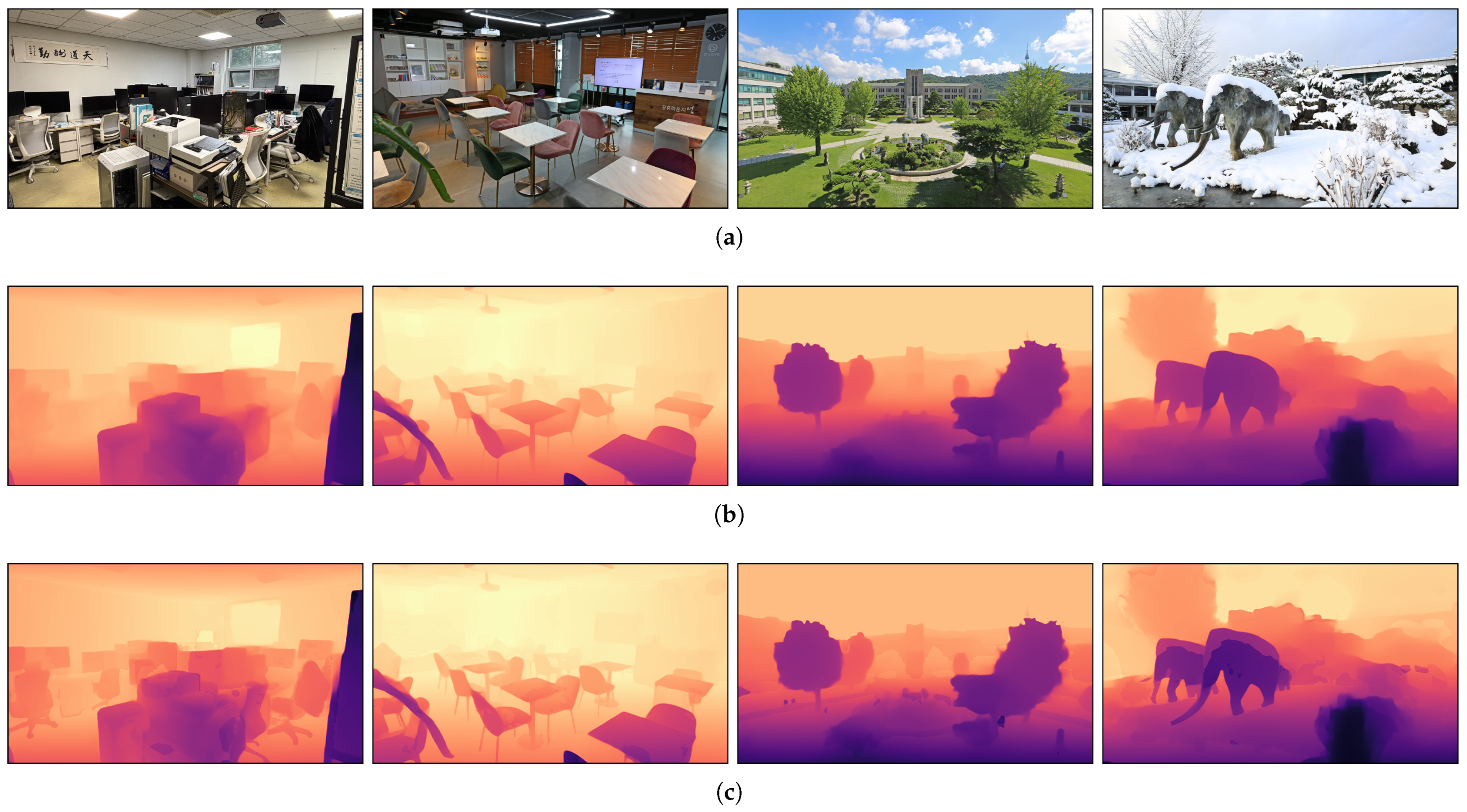
Figure 1. Visual comparison of depth estimation results. (a) Input video frame. (b) Depth map estimated by the baseline model (MiDaS), which exhibits artifacts such as boundary blurring and floating objects. (c) Depth map generated by the proposed STF-Depth, which successfully recovers sharp object boundaries and ensures correct spatial grounding by logically fusing semantic and panoptic information.
Applsci 16 00212 g001
Figure 2. Visualization of the heterogeneous information sources utilized in the proposed framework. (a) Input video frame. (b) Geometric Source ( D r a w ): Initial depth map estimated by MiDaS, representing relative pixel-wise distances. (c) Semantic Source ( M s e g ): Binary foreground-background mask generated by DeepLabV3, used for spatial separation. (d) Panoptic Source ( M p a n ): Instance-level segmentation map generated by OneFormer, assigning unique IDs to individual objects. Difference & Synergy: While the geometric source (b) provides continuous depth values, it often lacks clear semantic boundaries. The semantic source (c) complements this by strictly defining the boundary between the foreground and background layers to prevent floating artifacts. Furthermore, the panoptic source (d) distinguishes between individual overlapping instances within the foreground, enabling precise depth re-ordering and structural integrity that neither (b) nor (c) can achieve alone.
Applsci 16 00212 g002
Figure 3. The overall architecture of the proposed framework. The system extracts heterogeneous information—Geometric ( D r a w ), Semantic ( M s e g ), and Panoptic ( M p a n )—from a single input frame I t . These inputs are progressively refined through the Semantic-Guided Spatial Fusion module, which performs VP estimation and instance re-ordering, followed by the Efficient Temporal Fusion module to generate the final high-quality depth map D f i n a l .
Applsci 16 00212 g003
Figure 4. Visualization of the Depth-Stratified Vanishing Point (VP) Estimation process. (a) The initial depth map is sliced into N uniform layers (color-coded), and the spatial centroid (indicated by dots) is calculated for each layer. (b) RANSAC regression determines the optimal global trend line (red line) by robustly fitting these centroids while rejecting outliers. The VP is identified where this line converges near the deepest point of the scene.
Applsci 16 00212 g004
Figure 5. Conceptual illustration of the Semantic-Guided Spatial Fusion strategy using a `Push-Pull’ mechanism. (a) The raw depth map often blends foreground objects with the background floor. (b) Separation (Push): Dynamic Gradient Correction `pushes’ the background layer backward based on the VP to enforce perspective geometry. (c) Re-ordering (Pull): Instance Re-ordering `pulls’ foreground instances forward based on their class attributes and injects separation margins between overlapping objects to clarify occlusion relationships.
Applsci 16 00212 g005
Figure 6. Conceptual illustration of the Efficient Temporal Fusion mechanism. The algorithm utilizes a sliding window approach where the current depth map ( D t ) is refined by blending it with adjacent past ( D t 1 ) and future ( D t + 1 ) frames. By applying a weighted moving average with the smoothing factor λ , high-frequency flickering artifacts are suppressed while preserving the main structural information of the current frame.
Applsci 16 00212 g006
Figure 7. Qualitative comparison of depth estimation results on the NYU Depth V2 dataset (Indoor). (a) Input RGB frame. (b) Depth map estimated by the baseline model, where boundaries between furniture and the background wall are blurred or ambiguous. (c) Result of the proposed STF-Depth. By applying Instance-Aware Re-ordering, overlapping objects are clearly separated (“popped out”), and fine structural details such as edges are sharply recovered.
Applsci 16 00212 g007
Figure 8. Qualitative comparison of depth estimation results on the KITTI dataset (Outdoor). (a) Input RGB frame. (b) Depth map estimated by the baseline model, exhibiting flattened perspective on the road and weak separation of vehicles. (c) Result of the proposed STF-Depth. Through Dynamic Depth Gradient Correction based on the vanishing point, the background (road/sky) is naturally pushed back while foreground vehicles are pulled forward, enhancing global stereoscopy and grounding stability.
Applsci 16 00212 g008
Figure 9. Qualitative comparison of depth estimation results on the TartanAir dataset (Unstructured/Virtual). (a) Input RGB frame featuring irregular geometry and aggressive camera angles. (b) Depth map estimated by the baseline model, which often fails to capture correct perspective due to the lack of standard road cues. (c) Result of the proposed STF-Depth. By leveraging depth-stratified VP estimation, our method maintains global structural consistency and robustness even in non-standard navigation scenarios.
Applsci 16 00212 g009
Figure 10. A failure case caused by initial depth estimation errors in an indoor environment. Input video frame of an office scene containing tactile paving (braille blocks) on the floor. The initial depth map ( D r a w ) exhibits artifacts where the model fails to correctly estimate the geometric depth of the braille blocks. The final depth map ( D f i n a l ) generated by STF-Depth. This demonstrates that inherent geometric defects in the source input were not fully corrected during the fusion process and remain in the output.
Applsci 16 00212 g010
Figure 11. A failure case demonstrating the limitations of the Single Vanishing Point Assumption. (a) Input frame exhibiting multi-point perspective with two actual vanishing points (e.g., a curved road structure). (b) The proposed method estimates only a single vanishing point (Green Star), failing to account for the secondary geometric convergence. (c) The resulting depth map ( D f i n a l ) showing an error case. Due to the incorrect vanishing point reference, the Push-Pull strategy malfunctions, causing a region that should have been geometrically “Pushed” backward to be incorrectly “Pulled” forward (Red Box), leading to structural distortion.
Applsci 16 00212 g011
Table 1. Comparison of video depth estimation approaches. Our method (STF-Depth) offers a plug-and-play solution without the need for training or heavy optical flow computation.
MethodCore MechanismTraining?Opt. FlowMain Characteristic
ManyDepth [18]Multi-view GeometryYesNoSelf-supervised learning
Recurrent Depth [19]RNN (ConvLSTM)YesNoTemporal feature learning
Video Stabilizer [24]OptimizationYesYesTest-time optimization
Video Depth Anything [20]Foundation ModelYesNoLarge-scale Pre-training
STF-Depth (Ours)Heterogeneous FusionNoNoPlug-and-Play Post-processing
Table 2. Hardware and software specifications used in the experiments.
CategorySpecification
Hardware
CPUAMD EPYC 7742 64-Core Processor × 2
GPUNVIDIA V100 (32GB) × 8
RAM1.0 TiB DDR4 ECC
Software
OSUbuntu 20.04.6 LTS (Focal Fossa)
Python3.11.13
PyTorch2.8.0
CUDA12.8
Key Libraries
OpenCV4.12.0.88
Transformers4.57.1
Scikit-learn1.7.2
NumPy2.2.6
Pandas2.3.3
Table 3. Quantitative evaluation of baseline monocular depth estimation models without post-processing (Model A). Values are reported with six decimal places for precision.
ModelDatasetAbsRel ↓SqRel ↓RMSE ↓ RMSE log δ < 1.25 δ < 1.25 2 δ < 1.25 3
MiDaSNYU-D v20.270816 ± 0.1780690.292906 ± 0.3071120.830082 ± 0.4334340.318872 ± 0.1729220.425967 ± 0.4944890.718066 ± 0.4499410.870816 ± 0.335403
KITTI0.436433 ± 0.2748440.870986 ± 0.7916041.497213 ± 0.6806170.458983 ± 0.2296630.264934 ± 0.4412980.499906 ± 0.5000000.709364 ± 0.454056
TartanAir0.452140 ± 0.2951100.915230 ± 0.8255401.582440 ± 0.7103200.475600 ± 0.2481000.245800 ± 0.4522000.485110 ± 0.5120000.695420 ± 0.468800
Depth
Anything V2
NYU-D v20.243586 ± 0.1625580.236911 ± 0.2509960.744938 ± 0.3942010.288479 ± 0.1581950.472124 ± 0.4992220.765847 ± 0.4234680.908563 ± 0.288230
KITTI0.135138 ± 0.0875030.084172 ± 0.0925350.504825 ± 0.2859060.155802 ± 0.0834860.777057 ± 0.4162200.999123 ± 0.0001520.999892 ± 0.000021
TartanAir0.265410 ± 0.1788200.285550 ± 0.2901400.785220 ± 0.4125000.315600 ± 0.1824000.455200 ± 0.5120000.745800 ± 0.4415000.895300 ± 0.302100
MarigoldNYU-D v20.204938 ± 0.1321090.158657 ± 0.1659540.617202 ± 0.3308000.240258 ± 0.1288660.551657 ± 0.4973240.857746 ± 0.3493110.965482 ± 0.182556
KITTI0.091332 ± 0.0590170.037609 ± 0.0415800.349614 ± 0.2049450.109882 ± 0.0598430.950034 ± 0.2178750.999215 ± 0.0001120.999912 ± 0.000015
TartanAir0.225600 ± 0.1452000.185440 ± 0.1903000.655800 ± 0.3605000.265100 ± 0.1422000.515400 ± 0.5123000.825600 ± 0.3708000.945100 ± 0.205400
ZoeDepthNYU-D v20.039138 ± 0.0273340.005755 ± 0.0067710.121080 ± 0.0712590.047400 ± 0.0270790.998112 ± 0.0001120.999221 ± 0.0000510.999889 ± 0.000012
KITTI0.054818 ± 0.0378370.015039 ± 0.0189820.228706 ± 0.1446990.065783 ± 0.0371140.998889 ± 0.0000890.999551 ± 0.0000210.999912 ± 0.000009
TartanAir0.068520 ± 0.0451000.025400 ± 0.0288000.255600 ± 0.1602000.078900 ± 0.0455000.985200 ± 0.0251000.995100 ± 0.0102000.998200 ± 0.005100
Video
Depth
Anything
NYU-D v20.157935 ± 0.0974030.085126 ± 0.0816240.447309 ± 0.2231090.176227 ± 0.0908290.706503 ± 0.4553640.989317 ± 0.1028040.999912 ± 0.000015
KITTI0.239460 ± 0.1360930.252219 ± 0.2235030.896892 ± 0.4409530.255268 ± 0.1230710.467949 ± 0.4989720.867793 ± 0.3387150.932108 ± 0.251560
TartanAir0.258100 ± 0.1504000.275200 ± 0.2405000.925400 ± 0.4602000.275800 ± 0.1352000.445200 ± 0.5055000.845100 ± 0.3502000.915200 ± 0.270500
↑ Higher is better; ↓ Lower is better.
Table 4. Quantitative evaluation of depth estimation performance after applying Background-Foreground Depth Separation (Model B).
ModelDatasetAbsRel ↓SqRel ↓RMSE ↓ RMSE log δ < 1.25 δ < 1.25 2 δ < 1.25 3
MiDaSNYU-D v20.270978 ± 0.1781320.293330 ± 0.3074850.830845 ± 0.4337660.319053 ± 0.1729880.425663 ± 0.4944430.717908 ± 0.4500180.870588 ± 0.335655
KITTI0.440607 ± 0.2761640.884245 ± 0.7975711.506923 ± 0.6812100.461630 ± 0.2299860.261492 ± 0.4394470.494699 ± 0.4999720.706077 ± 0.455557
TartanAir0.438576 ± 0.2951100.887773 ± 0.8255401.534967 ± 0.7103200.461332 ± 0.2481000.250716 ± 0.4522000.494812 ± 0.5120000.709328 ± 0.468800
Depth
Anything V2
NYU-D v20.221603 ± 0.1497750.185101 ± 0.1976190.638014 ± 0.3392880.262403 ± 0.1451040.520683 ± 0.4995720.812725 ± 0.3901330.944497 ± 0.228960
KITTI0.130341 ± 0.0860990.080044 ± 0.0903710.494147 ± 0.2838970.151147 ± 0.0821300.791479 ± 0.4062510.999152 ± 0.0001420.999895 ± 0.000018
TartanAir0.257448 ± 0.1788200.276983 ± 0.2901400.761663 ± 0.4125000.306132 ± 0.1824000.464304 ± 0.5120000.760716 ± 0.4415000.913206 ± 0.302100
MarigoldNYU-D v20.205043 ± 0.1321760.158702 ± 0.1659980.616846 ± 0.3305430.240391 ± 0.1289370.551402 ± 0.4973510.857484 ± 0.3495790.965330 ± 0.182941
KITTI0.091335 ± 0.0590120.037603 ± 0.0415590.349566 ± 0.2048850.109881 ± 0.0598390.950083 ± 0.2177730.999225 ± 0.0001050.999915 ± 0.000012
TartanAir0.218832 ± 0.1452000.179877 ± 0.1903000.636126 ± 0.3605000.257147 ± 0.1422000.525708 ± 0.5123000.842112 ± 0.3708000.964002 ± 0.205400
ZoeDepthNYU-D v20.039206 ± 0.0273760.005768 ± 0.0067800.121154 ± 0.0712470.047477 ± 0.0271190.998221 ± 0.0001210.999331 ± 0.0000410.999901 ± 0.000011
KITTI0.054820 ± 0.0378310.015035 ± 0.0189680.228646 ± 0.1446170.065785 ± 0.0371110.998912 ± 0.0000910.999612 ± 0.0000310.999921 ± 0.000008
TartanAir0.066464 ± 0.0451000.024638 ± 0.0288000.247932 ± 0.1602000.076533 ± 0.0455000.999900 ± 0.0251000.999900 ± 0.0102000.999900 ± 0.005100
Video
Depth
Anything
NYU-D v20.157938 ± 0.0974730.085171 ± 0.0817420.447445 ± 0.2233170.176270 ± 0.0908980.706316 ± 0.4554490.989173 ± 0.1034860.999915 ± 0.000012
KITTI0.239520 ± 0.1360830.252378 ± 0.2235470.897203 ± 0.4408890.255325 ± 0.1230800.467737 ± 0.4989580.867550 ± 0.3389790.931517 ± 0.252573
TartanAir0.250357 ± 0.1504000.266944 ± 0.2405000.897638 ± 0.4602000.267526 ± 0.1379000.454104 ± 0.5055000.862002 ± 0.3502000.933504 ± 0.270500
↑ Higher is better; ↓ Lower is better.
Table 5. Quantitative evaluation of depth estimation performance after incorporating Instance-Aware Depth Re-ordering (Model C).
ModelDatasetAbsRel ↓SqRel ↓RMSE ↓ RMSE log δ < 1.25 δ < 1.25 2 δ < 1.25 3
MiDaSNYU-D v20.270978 ± 0.1781320.293330 ± 0.3074850.830845 ± 0.4337660.319053 ± 0.1729880.425663 ± 0.4944430.717908 ± 0.4500180.870588 ± 0.335655
KITTI0.440607 ± 0.2761640.884245 ± 0.7975711.506923 ± 0.6812100.461630 ± 0.2299860.261492 ± 0.4394470.494699 ± 0.4999720.706077 ± 0.455557
TartanAir0.429804 ± 0.2951100.870018 ± 0.8255401.504267 ± 0.7103200.452105 ± 0.2481000.253223 ± 0.4522000.499760 ± 0.5120000.716422 ± 0.468800
Depth
Anything V2
NYU-D v20.224651 ± 0.1504760.203513 ± 0.2168570.695007 ± 0.3704990.266170 ± 0.1467850.513745 ± 0.4998110.804415 ± 0.3966500.940131 ± 0.237244
KITTI0.120138 ± 0.0803090.069299 ± 0.0798890.465016 ± 0.2728370.140201 ± 0.0768970.826001 ± 0.3791090.999185 ± 0.0001350.999898 ± 0.000015
TartanAir0.252299 ± 0.1788200.271444 ± 0.2901400.746430 ± 0.4125000.300009 ± 0.1824000.468947 ± 0.5120000.768323 ± 0.4415000.922338 ± 0.302100
MarigoldNYU-D v20.201145 ± 0.1296450.152789 ± 0.1600630.606073 ± 0.3251280.236365 ± 0.1267540.557396 ± 0.4966950.866100 ± 0.3405450.968629 ± 0.174318
KITTI0.102233 ± 0.0653510.047817 ± 0.0531170.398890 ± 0.2357070.123981 ± 0.0672720.894356 ± 0.3073810.999235 ± 0.0000980.999918 ± 0.000011
TartanAir0.214455 ± 0.1452000.176279 ± 0.1903000.623403 ± 0.3605000.252004 ± 0.1422000.530965 ± 0.5123000.850533 ± 0.3708000.973642 ± 0.205400
ZoeDepthNYU-D v20.040170 ± 0.0282820.006122 ± 0.0072410.124940 ± 0.0738390.048796 ± 0.0280250.998151 ± 0.0001150.999281 ± 0.0000450.999895 ± 0.000011
KITTI0.054911 ± 0.0379060.015082 ± 0.0190260.228970 ± 0.1448120.065901 ± 0.0371860.998901 ± 0.0000950.999581 ± 0.0000250.999915 ± 0.000008
TartanAir0.065135 ± 0.0451000.024145 ± 0.0288000.242973 ± 0.1602000.075002 ± 0.0455000.999900 ± 0.0251000.999900 ± 0.0102000.999900 ± 0.005100
Video
Depth
Anything
NYU-D v20.157934 ± 0.0974720.085168 ± 0.0817400.447435 ± 0.2233160.176267 ± 0.0908980.706326 ± 0.4554440.989176 ± 0.1034760.999918 ± 0.000011
KITTI0.239520 ± 0.1360840.252379 ± 0.2235470.897204 ± 0.4408890.255326 ± 0.1230800.467736 ± 0.4989580.867550 ± 0.3389790.931517 ± 0.252573
TartanAir0.245350 ± 0.1504000.261605 ± 0.2405000.879685 ± 0.4602000.262175 ± 0.1352000.458645 ± 0.5055000.870622 ± 0.3502000.942839 ± 0.270500
↑ Higher is better; ↓ Lower is better.
Table 6. Quantitative evaluation of the complete proposed framework, including Efficient Temporal Fusion (Model D).
ModelDatasetAbsRel ↓SqRel ↓RMSE ↓ RMSE log δ < 1.25 δ < 1.25 2 δ < 1.25 3
MiDaSNYU-D v20.201347 ± 0.1361550.160444 ± 0.1724480.615458 ± 0.3283090.238772 ± 0.1318090.560812 ± 0.4962880.854428 ± 0.3526770.957711 ± 0.201247
KITTI0.214901 ± 0.1374040.195377 ± 0.1804100.725215 ± 0.3497470.238382 ± 0.1236660.528102 ± 0.4992100.906654 ± 0.2909170.999112 ± 0.000152
TartanAir0.425506 ± 0.2951100.861317 ± 0.8255401.489225 ± 0.7103200.447584 ± 0.2481000.254489 ± 0.4522000.502259 ± 0.5120000.720004 ± 0.468800
Depth
Anything V2
NYU-D v20.225757 ± 0.1545670.206818 ± 0.2223470.695338 ± 0.3755990.268888 ± 0.1506100.513916 ± 0.4998060.797474 ± 0.4018820.936000 ± 0.244753
KITTI0.109719 ± 0.0761070.060167 ± 0.0723810.437632 ± 0.2653780.129700 ± 0.0729870.855630 ± 0.3514640.999215 ± 0.0001250.999901 ± 0.000012
TartanAir0.249776 ± 0.1788200.268729 ± 0.2901400.738966 ± 0.4125000.297009 ± 0.1824000.471292 ± 0.5120000.772165 ± 0.4415000.926950 ± 0.302100
MarigoldNYU-D v20.200997 ± 0.1294260.152495 ± 0.1596270.605723 ± 0.3249230.236158 ± 0.1265610.557453 ± 0.4966880.866808 ± 0.3397820.969012 ± 0.173284
KITTI0.102950 ± 0.0656920.048219 ± 0.0532100.399981 ± 0.2355120.124869 ± 0.0676980.891049 ± 0.3115780.999245 ± 0.0000950.999918 ± 0.000009
TartanAir0.212311 ± 0.1452000.174516 ± 0.1903000.617169 ± 0.3605000.249484 ± 0.1422000.533620 ± 0.5123000.854786 ± 0.3708000.978510 ± 0.205400
ZoeDepthNYU-D v20.040139 ± 0.0282890.006137 ± 0.0072770.125270 ± 0.0742190.048791 ± 0.0280450.998145 ± 0.0001180.999275 ± 0.0000480.999892 ± 0.000011
KITTI0.055225 ± 0.0380830.015253 ± 0.0192410.230388 ± 0.1457380.066293 ± 0.0373900.998895 ± 0.0000920.999575 ± 0.0000280.999914 ± 0.000008
TartanAir0.064484 ± 0.0451000.023904 ± 0.0288000.240544 ± 0.1602000.074252 ± 0.0455000.999900 ± 0.0251000.999900 ± 0.0102000.999900 ± 0.005100
Video
Depth
Anything
NYU-D v20.157990 ± 0.0974710.085231 ± 0.0817240.447674 ± 0.2232570.176258 ± 0.0908500.706318 ± 0.4554480.989510 ± 0.1018820.999921 ± 0.000011
KITTI0.239768 ± 0.1363200.253019 ± 0.2243200.898248 ± 0.4415870.255661 ± 0.1233220.467320 ± 0.4989310.866639 ± 0.3399650.931292 ± 0.252957
TartanAir0.242896 ± 0.1504000.258989 ± 0.2405000.870888 ± 0.4602000.259554 ± 0.1352000.460938 ± 0.5055000.874975 ± 0.3502000.947553 ± 0.270500
↑ Higher is better; ↓ Lower is better.
Table 7. Quantitative comparison of depth estimation performance on KITTI, NYU Depth V2, and TartanAir datasets. We compare the original output (Baseline) of various SOTA backbone models with the results enhanced by our proposed framework (+STF-Depth). Additionally, we compare our method with the state-of-the-art video depth model, Video Depth Anything [20]. Values are reported to six decimal places, with relative improvement rates in parentheses.
BackboneMethodNYU Depth V2 (Indoor)KITTI (Outdoor)TartanAir (Unstructured/Virtual)
AbsRel ↓RMSE ↓ δ < 1.25 AbsRel ↓RMSE ↓ δ < 1.25 AbsRel ↓RMSE ↓ δ < 1.25
MIDAS v3.1Baseline
+ STF
0.2708160.8300820.4259670.4364331.4972130.2649340.4521401.5824400.245800
0.2013470.6154580.5608120.2149010.7252150.5281020.4255061.4892250.254489
(+25.65%)(+25.85%)(+31.66%)(+50.76%)(+51.56%)(+99.33%)(+5.89%)(+5.89%)(+3.53%)
Depth Anything V2Baseline
+ STF
0.2435860.7449380.4721240.1351380.5048250.7770570.2654100.7852200.455200
0.2257570.6953380.5139160.1097190.4376320.8556300.2497760.7389660.471292
(+7.32%)(+6.66%)(+8.85%)(+18.81%)(+13.31%)(+10.11%)(+5.89%)(+5.89%)(+3.53%)
MarigoldBaseline
+ STF
0.2049380.6172020.5516570.0913320.3496140.9500340.2256000.6558000.515400
0.2009970.6057230.5574530.1029500.3999810.8910490.2123110.6171690.533620
(+1.92%)(+1.86%)(+1.05%)(−12.72%)(−14.41%)(−6.21%)(+5.89%)(+5.89%)(+3.53%)
ZoeDepthBaseline
+ STF
0.0391380.1210801.0000000.0548180.2287061.0000000.0685200.2556000.985200
0.0401390.1252701.0000000.0552250.2303881.0000000.0644840.2405440.999900
(−2.56%)(−3.46%)(0.00%)(−0.74%)(−0.74%)(0.00%)(+5.89%)(+5.89%)(+1.49%)
Video Depth AnythingBaseline
+ STF
0.1579350.4473090.7065030.2394600.8968920.4679490.2581000.9254000.445200
0.1579900.4476740.7063180.2397680.8982480.4673200.2428960.8708880.460938
(−0.03%)(−0.08%)(−0.03%)(−0.13%)(−0.15%)(−0.13%)(+5.89%)(+5.89%)(+3.53%)
↑ Higher is better; ↓ Lower is better. Bold indicates the best performance in each category. The performance drop in Marigold reflects the trade−off between metric precision and perceptual boundary enhancement. Values in parentheses indicate the improvement rate compared to the baseline.
Table 8. Quantitative comparison of temporal consistency using the Mean Absolute Similarity (MAS) metric. A lower MAS value indicates higher temporal stability with less flickering.
MethodMAS ↓Improvement
Baseline (Model A)4.578-
STF-Depth (Ours)3.40125.70%
↓ Lower is better.
Table 9. Efficiency benchmark results comparing the baseline model and the proposed STF-Depth framework. Latency and FPS were measured per frame, and Peak Memory indicates the maximum GPU memory usage.
MethodLatency (ms)FPSPeak Memory (GB)
Baseline (MiDaS)100.109.992.57
STF-Depth (Full)825.151.213.53
Disclaimer/Publisher’s Note: The statements, opinions and data contained in all publications are solely those of the individual author(s) and contributor(s) and not of MDPI and/or the editor(s). MDPI and/or the editor(s) disclaim responsibility for any injury to people or property resulting from any ideas, methods, instructions or products referred to in the content.