Article

Honey Bee Lifecycle Activity Prediction Using Non-Invasive Vibration Monitoring

1
Department of Acoustics, Multimedia and Signal Processing, Wrocław University of Science and Technology, 27 Wybrzeże Stanisława Wyspiańskiego St., 50-370 Wrocław, Poland
2
Division of Apiculture, Wrocław University of Environmental and Life Sciences, Norwida 25 St., 50-375 Wrocław, Poland
*
Author to whom correspondence should be addressed.
Appl. Sci. 2026, 16(1), 188; https://doi.org/10.3390/app16010188
Submission received: 17 November 2025 / Revised: 4 December 2025 / Accepted: 23 December 2025 / Published: 24 December 2025
(This article belongs to the Special Issue The World of Bees: Diversity, Ecology and Conservation)

Abstract

Honey bees are essential both for many global ecosystems and apicultural production. The management of bee colonies remains labour-intensive, which drives a need for automated solutions. This work presents a proof-of-concept system to monitor honey bee activity by identifying the yearly lifecycle stages exhibited by the colony. A non-invasive vibration monitoring system was developed and placed on top of brood frames in Warsaw-type beehives to collect vibration data over a full apicultural season. The recorded vibration signals were analyzed using both Convolutional Neural Networks (CNNs) and classical machine learning approaches such as the extra trees method. Recursive Feature Elimination with Cross-Validation (RFECV) was performed to isolate the most important frequency bins for lifecycle period identification. The results demonstrate that the critical frequencies for recognizing yearly honey bee activity are concentrated below 1 kHz. The proposed machine learning models achieved a weighted accuracy score of over 95%. These findings have significant implications for future bee monitoring hardware design, indicating that sampling frequencies may be reduced to as low as 2 kHz without significantly compromising model accuracy.

1. Introduction

The honey bee colony is a superorganism, exhibiting complex behaviour dependent on many factors ranging from the environment to the state of the colony itself. Bee products such as honey, pollen and propolis are used widely both in consumer goods and in the industry in many use-cases. Bees are also important pollinators, crucial to many ecosystems around the world. Bees are tended to by beekeepers, who use specialised tools and techniques for the upkeep of their colonies, including monitoring the state of the colony.
Monitoring honey bee colonies can be performed using many techniques, starting with the simplest practice of manual inspection. Manual inspection of bee colonies allows for an overview of the overall colony’s state, strength, honey reserves and brood status. In classical apiculture, in large apiaries, this is the preferred way of managing large numbers of bee colonies. This approach, however, is labour intensive and requires expert beekeepers to perform inspections for best results, which comes with great costs. One of the solutions to improve upon the manual nature of beekeeping is automation, specifically automated honey bee colony monitoring via Internet of Things (IoT) applications [1,2].
The growing availability of digital tools does not straightforwardly translate to their adoption in apicultural practice. According to some reports around 71% [3] to 79% [4] of beekeepers do not use any digital tools, while those utilising such techniques, most often simply use an apiary scale. IoT, combined with artificial intelligence (AI), allows for the non-invasive monitoring of bee colony conditions by integrating different sensors such as those measuring temperature, humidity, CO2, and colony weight, and can even include video surveillance of the beehive entrance [5,6]. Using such data, the real-time tracking of the internal colony microclimate as well as early threat detection become possible [7,8]. Data collected during such monitoring can aid in decision-making and allow for a reduction in manual inspections. The crucial aspect of bee monitoring is monitoring the bees in a non-invasive way, to allow for natural behavioural patterns to occur [5].
Automated bee colony monitoring with sound and vibration signals recorded inside the beehive has shown great promise as an expanding field bordering on machine learning, the natural sciences and engineering. The relationship between bees and sound has been studied for decades, with seminal works including those authored by Dreller and Kirchner et al., who provide information regarding the response of the Johnston’s organ to sound excitation [9,10]. Vibration has also been investigated, with works showing that the waggle dance contains informative vibroacoustic data, which is interpretable by honey bees [11]. More recently, it has been found that active worker bees produce low-frequency vibration, which does not transfer well to hive structures [12]. The honey bee thorax has also been analysed numerically to locate the important fundamental frequencies, as they may be connected with the wing beat frequency of bees ventilating the hive and in bee flight [13].
Recent works regarding bee colonies produced by Ramsey et al., focused on monitoring the bee colony with high-precision acceleration sensors, have provided insight into the trends of the honey bee whooping signal over extended time periods [14]. The team’s analyses have also found that it may be possible to identify bee swarming based on the vibration signals recorded inside beehives, as well as the prediction of swarming behaviours using similar techniques [15]. Vibration produced by bees when preparing for greater activity is known as Dorso-Ventral Abdominal Vibration (DVAV). Such signals were studied by Ramsey et al. and have been shown to be present in multiple bee colonies located in multiple countries, and can also be understood to be a swarming event predictor [16].
In addition to vibration signals, sounds are also of interest to automated monitoring tasks, with multiple works focusing on different aspects of bee health and wellbeing. Often such works incorporate machine learning methods, providing classifiers for different classification problems. Such problems include detecting the presence of the queen bee [17,18], identifying swarming events [19,20], making distinctions between bee and non-bee signals [21] and differentiating between worker bees and drones [22]. In the field, microphones are placed both inside and outside the beehive, with internal microphone placement having the main drawback of propolis and beeswax build-up on instruments, which impacts the effectiveness of the research and the results of measurements [23,24] and may be one of the causes limiting large-scale adoption of such systems [25].

1.1. Honey Bee Colony Lifecycle

Honey bees live in diverse environments with different climates. In a temperate climate, the lifecycle of the bee colony can be divided into several stages that can be differentiated by the physiological state of the colony as well as bee activity [26]. Knowledge of the biology of the colony during specific phases of the cycle is key to correct decision-making in apiary management.
From the last autumn flight to the first spring flight, the colony is considered to be in a state of wintering. During this time, the hive is empty of brood and bees clump together to form a cluster and lower the temperature inside the cluster to around 20 °C, which causes a significant slow-down of the bee metabolism. During this time bees are somewhat protected from certain threats, as Varroa destructor mites do not multiply due to a lack of a brood in the hive. In the second half of the winter, when environmental temperatures reach around 4 °C [26], the temperature inside the cluster rises to 34 °C and the queen begins laying a new brood, which will be reared for spring. When the temperature reaches and stays at around 10 °C to 12 °C during the day, bees leave the hive and perform a cleansing spring flight, which marks the start of the second stage in the colony lifecycle—the change from wintering bees to spring bees.
In the early spring the queen intensively lays new eggs and the colony changes its composition, with old bees dying and young workers taking over. This can cause the size of the colony to fluctuate, even possibly causing it to decrease. This stage takes around 6 weeks from the first spring flight. When the family is clear of overwintered bees, and the brood laying speed of the queen does not slow, the number of bees in the colony rises and reaches its peak in the middle of spring. This is the growth stage of the honey bee colony, which leads directly to the main production stage.
In the production stage, the colony’s strength, as well as the age structure of bees in the colony, is of great significance. Optimally, the colony should have as many young forager bees and worker bees focusing on processing the materials gathered by foragers. In this stage, if forage becomes poor (gaps in forage), the colony may perform swarming. Such a situation is unfortunate, as the honey yields from swarming colonies drop drastically, which impacts the apicultural economy negatively. During significant production, the queen lowers the brooding rate, which leads to a lowered colony strength after the production stage ends.
At the end of summer, the colony again starts rising in numbers in preparation for overwintering. Around the middle of September, the queen bee should stop laying new eggs, and in mid-October, the colony should be brood-free, so the workers can physiologically prepare for overwintering, which starts when the average daily temperature falls below 9 °C [27].
Identification of bee colony lifecycle periods is a crucial part of managed, proactive beekeeping practices. One of the possible avenues for automation in such a case would be a decision-assisting method providing insight into the bee colony’s state based on measurable parameters such as sound or vibration.

1.2. Our Approach

Due to the difficulties of invasive measurement techniques, our approach in this work was to develop a prototype IoT-enabled system for honey bee vibration monitoring designed from the ground up to be wholly non-invasive as well as universal in its construction. The system was built specifically to record the year-round vibration of the beehive structure in order to verify the feasibility of using such a device for monitoring bee behaviour. For this purpose, we elected to monitor the vibration for a period of nine months, divide the lifecycle of the bee colony into five distinct stages and use machine learning methods to perform the classification of the honey bee lifecycle based on measurements from two bee colonies. Additionally, we performed signal origin classification to differentiate between signals recorded in both hives in order to verify the viability of such a task and to locate potential issues that may affect further work.
In our experiment, we verified the importance of given frequencies for both stated tasks to locate potential savings in sampling frequency for non-invasive monitoring. To this end we utilised state-of-the-art feature selection methods as well as verification on a filtered dataset. The specific contributions of this work are as follows:
1.
The creation of a honey bee vibration dataset spanning a whole apicultural season, recorded using wholly non-invasive techniques with accelerometers positioned on top of brood frames.
2.
Performance of lifecycle period identification using convolutional neural networks along with logistic regression and extra trees methods.
3.
Feature importance analysis of honey bee-produced vibration for the task of lifecycle period classification and hive identification; verification of the conclusions using a band-filtered dataset.
4.
An analysis of possible difficulties affecting further experiments regarding bee colony identification using vibration signals recorded in beehives.
The following sections are structured as follows. Section 2 describes the measurement station design, dataset preparation and both the classification methods used and the feature importance analysis process. Section 3 contains the results of the experiment, while Section 4 shows the discussion of the results and Section 5 describes the conclusions and future work to be conducted in the field.

2. Materials and Methods

To achieve the stated goal of lifecycle period recognition, a measurement set-up was devised. Then, measurements were performed over the course of the year in two bee colonies placed in the same type of beehive and at the same apiary. Subsequently, data features were extracted and classification was performed using convolutional neural networks, Perceptron-Based Neural Networks as well as extra trees classifiers. Feature importance analysis was carried out using the RFECV method with an extra trees classifier as the test model. Additionally, the analysis was also performed for the task of hive identification. All analyses were repeated on a filtered dataset.

2.1. Measurement Set-Up

The measurement set-up used in the experiment was a dedicated IoT-enabled device made specifically for monitoring beehive vibration. The device, called the Bee Activity Detector, is based on the ESP32-WROOM-32 module, and is a prototype meant specifically for the verification of the possibility for honey bee colony state monitoring based on a low-cost acceleration sensor.
A diagram of the device is shown in Figure 1. The power supply for the station was positioned at a distance of 30 m from the beehives, in a utility building. This distance was necessitated by the higher supply voltage and the inclusion of a step-down board in the device to ensure a sufficiently stable power supply for measurements. Communication between the ESP32 and the SD card, as well as the ADXL355 accelerometer is performed using the SPI protocol at a speed of 40 MHz for stability. Both devices are placed on separate SPI buses, as the communication is performed concurrently to both devices during measurement. Communication with the DS3231 RTC module is realised via the I2C protocol.
The measurement station is implemented using FreeRTOS with two programmed tasks. The first task is responsible for handling the communication with ADXL355, setting up the sensor and reading the data from FIFO queue on the accelerometer. The second task handles the file saving, as well as the RTC module for timestamping. Communication between tasks is performed using a Queue system passing structural objects with vibration data, as well as control information. Each buffer passed through the queue contains 32 signal frames, each of which contains 16 24-bit samples of X, Y and Z vibration. The files are saved to a custom, headless C-struct-defined binary format with the extension .bzz, containing the tri-axis measurement and temperature data for sensitivity correction and timestamping, as well as a FIFO overflow flag in case of errors with data reads from ADXL resulting in a FIFO queue overflow and lost samples. A Python 3.11 script was developed for reading these files and was used for data extraction in this experiment.
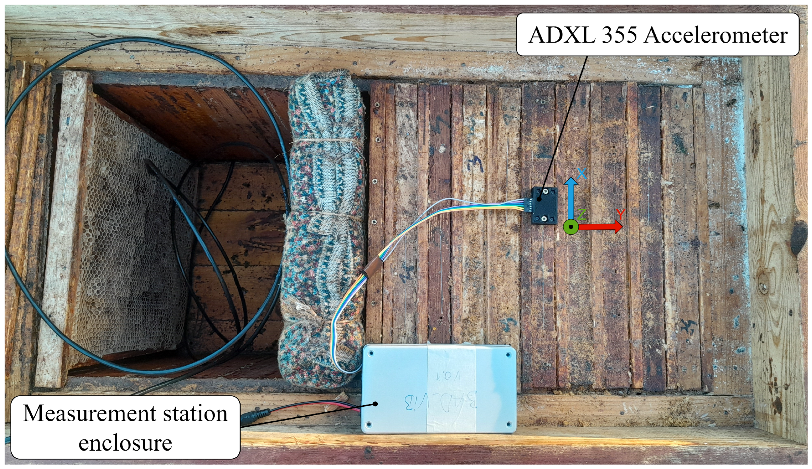
Measurement stations were mounted on bee colonies in late January 2025, with measurements starting on 1 February 2025. The positioning of acceleration sensors was identical in both colonies with sensors placed off-centre on a brood frame, where the highest temperature was detected. Figure 2 shows the measurement set-up mounted on hive 1. The Z axis is positioned in the normal direction of the frame-top plane, with the X and Y axes being orthogonal and parallel to the bee frame stacking direction, respectively. Measurements were made with a sampling frequency of 4 kHz. Measurements were performed for periods of 20 s, beginning at the start of each minute, with measurements performed in both hives simultaneously.

2.2. Dataset Preparation

The dataset used for training classification methods was composed of vibration recordings made between the 1 February 2025 and 25 October 2025, comprising a full apicultural season and bee colony lifecycle.
The recordings, due to ongoing developmental work and issues with power delivery to the apiary, were not fully continuous, with maintenance and power delivery causing gaps between them. The gaps in the recording, while not evenly spaced in time, were not correlated with any local natural phenomena and, as such, are unlikely to introduce significant bias into the dataset. The only category significantly affected by the outages is the winter preparation category, as significant measurement outages occurred between 17 August and 31 August as well as between 14 September and 4 October, and were caused by equipment failures affecting both measurement stations. A partial outage was also present during the growth phase (6 April to 13 April) and the early production phase (18 May to 23 May). Figure 3 shows all lifecycle periods used for the classification problem along with highlights showing weeks during which outages occurred. Outage periods provided no data that could be used in this experiment. The overall dataset is composed of 146,182 recordings, with 75,506 originating from the first studied colony and 70,676 originating from the second colony. In this experiment, both measured beehives contained apparently healthy Apis mellifera carnica colonies.
Throughout the year, notes made on the availability of bee sustenance sources and colony health. Colony health over the measurement period was judged to be good, and both measured colonies exhibited expected behavioural patterns over the year, with the greatest activity levels exhibited in late spring, as the greatest nectar yields can be found between early May and late June at the location where the apiary is situated. The colonies were isolated from adverse vibroacoustic stressors, as the orchard in which they were located was far from agricultural and industrial sources of vibroacoustic excitation. The season during which the measurements were performed did not show any signs of significant deviation from meteorological expectations for the region, with the meteorological considerations discussed in Appendix A. Queens were exchanged during the season in both colonies in early June, with new queens being accepted by the colonies without issue. Varroa treatments applied via smoking were performed in the spring and autumn according to standard beekeeping practice with two Apiwarol (Amitraz) treatments applied in March and three treatments in September. No treatments were performed during production stages, as it was not deemed necessary. The effect on vibration signals produced by the colonies during and after treatments was short-term, and as such was not considered to be a factor in this analysis. Figure 4 shows the approximate plant blooming and nectar yield periods through the year in the vicinity of the apiary, as observed in the apiary notes.
For the task of colony state estimation, the yearly lifecycle of the honey bee colonies in the context of this work was divided into five distinct phases, which were the classes used in the classification problem. The category definitions can be seen in Table 1. The dates used for determining the classification labels were provided by the beekeeper tending to the apiary based on manual observation of the brood count, colony strength, nectar store status and the number of dead bees at the hive entrances. The beekeeper informed the categorical split unaware of the results achieved in the measurements. The classification categories were also impacted by the forage availability in the area around the apiary, informing the split of the production phase into early and late production. Events categorising the lifecycle period of honey bees informing the categorical split are described in greater detail in Section 1. Each category begins and ends at midnight of the respective boundary day. There are no overlapping classification periods.
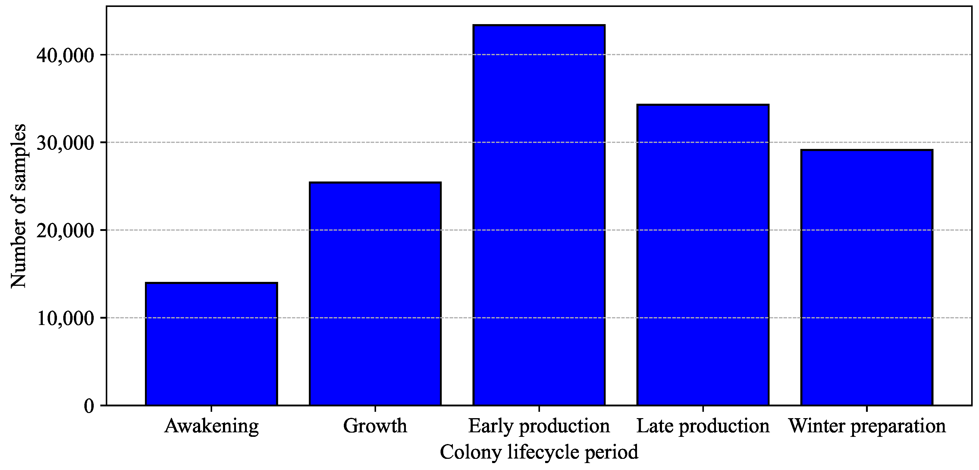
Categorisation of the dataset into five classes provided a machine learning dataset with uneven class counts stemming from the different lengths of each lifecycle period as well as maintenance breaks. Figure 5 shows the category count for each class used in the experiment. In all following work, care was taken to account for this uneven class distribution.
As a first step in analysis, the vibration data was analysed using fundamental frequency recognition based on signal autocorrelation. The features were extracted for each recorded sample per channel, with the signal filtered using a 10th-order bandpass Butterworth filter with the low cut-off frequency being 100 Hz and the upper cut-off frequency being 550 Hz. The fundamental frequency, a method often used in speech analysis [28], can be calculated as seen in Equation (1), where τ z m a x is the time delay required to achieve the maximum autocorrelation value, excluding the trivial τ = 0 , in a continuous signal, while k z m a x is the equivalent for discrete signals—the sample delay required for the maximum autocorrelation function value. For discrete signals f s is the sampling frequency. In this analysis, parabolic interpolation was used to increase the frequency resolution of the method by approximating non-integer k z m a x values.
F 0 = 1 τ z m a x = f s k z m a x
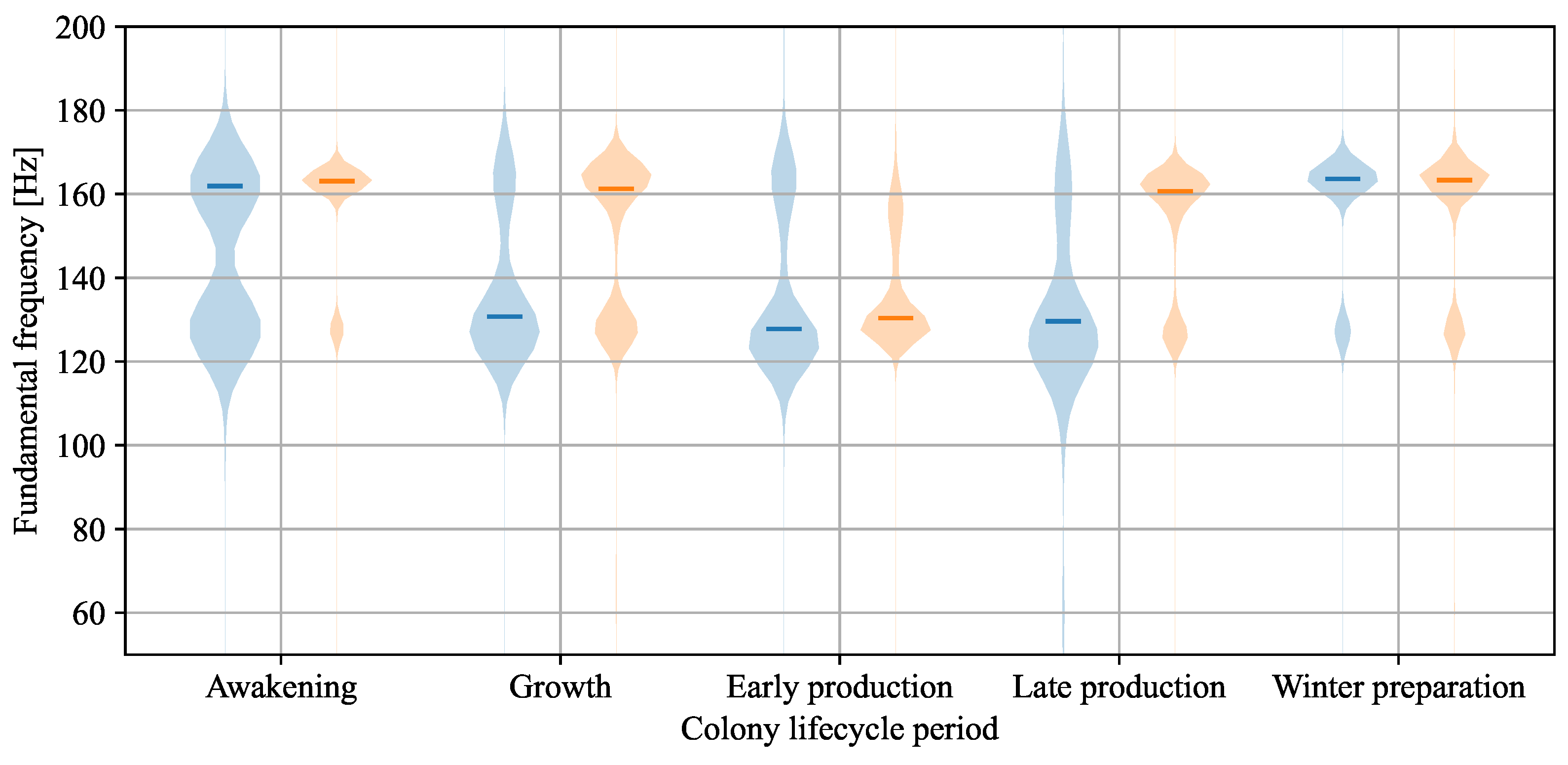
Figure 6 shows the distributions of fundamental frequency values grouped by both the lifecycle period and the colony from which the distribution originates. The graph shows that there are differences between signals recorded at different times during the year, and, as such, differentiation of the lifecycle period based on vibration data analysis was deemed to be likely to be achievable. Interestingly, there are also differences between the colonies in which recordings were made, especially in the growth and late production phases. As such, it was decided that the identification of the colonies, based on vibration data, would also be performed as an additional analysis.
For the purpose of classification, the extracted feature chosen was the power spectrum calculated via Welch’s method [29]. Power spectra were calculated with an 800-sample Hanning window with a 50% overlap. This process was performed for all three data channels. The channel spectra were subsequently vector summed to create a single feature vector invariant to the vibration direction, providing a data vector with 401 parameters and a single channel.
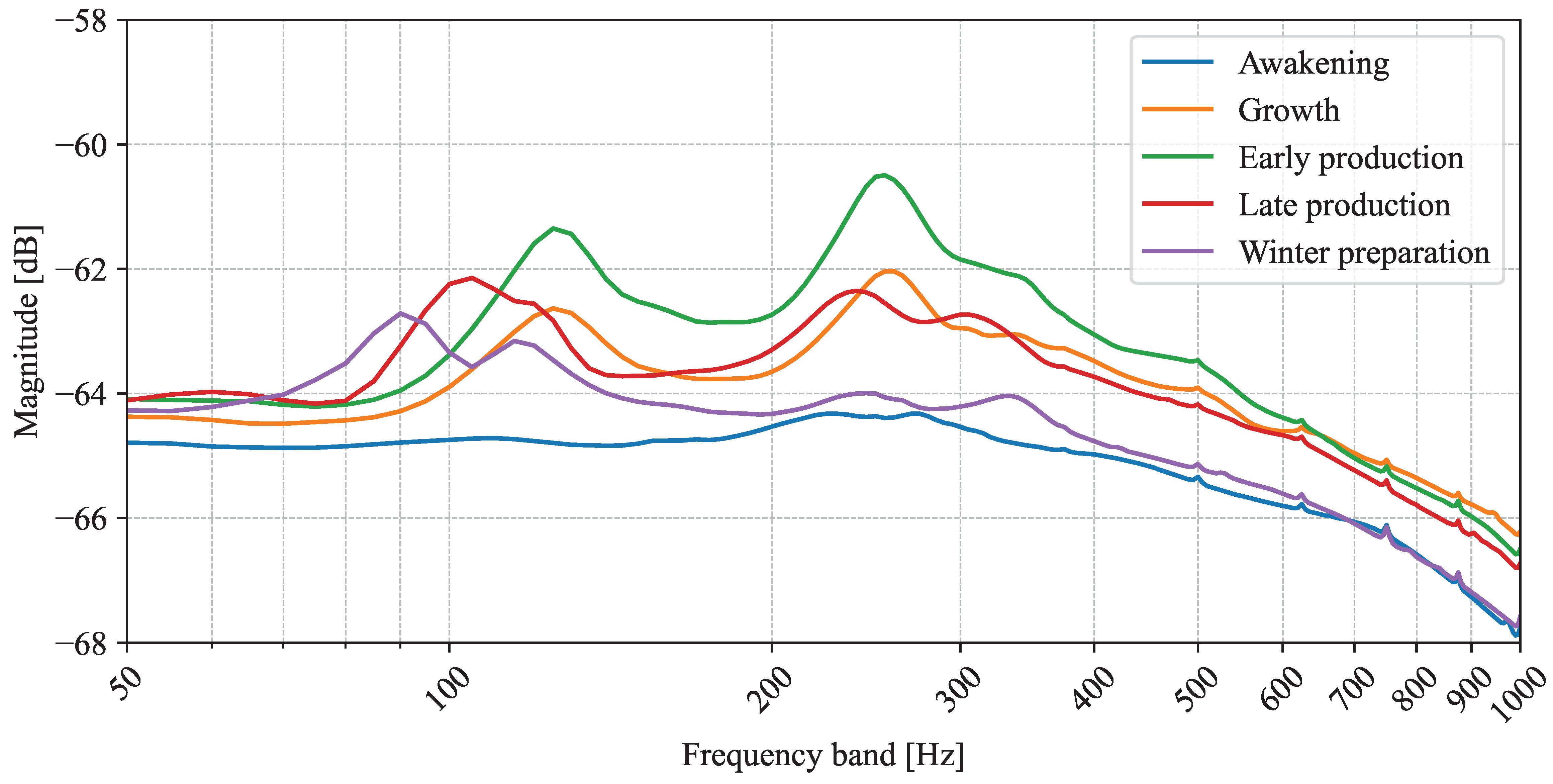
Similarly to the fundamental frequency analysis, Figure 7 shows the averaged spectral information per colony lifecycle change. It can be seen that the spectral contents of the signal depend strongly on the lifecycle period when the recordings are acquired. The spectral contents of the early production stage most closely represent the commonly understood model of working honey bee sound and vibration, with two significant bins—one between 100 and 200 Hz and one between 200 and 300 Hz [13,30]. The early production peaks also reach higher amplitudes, showing an increase in activity.
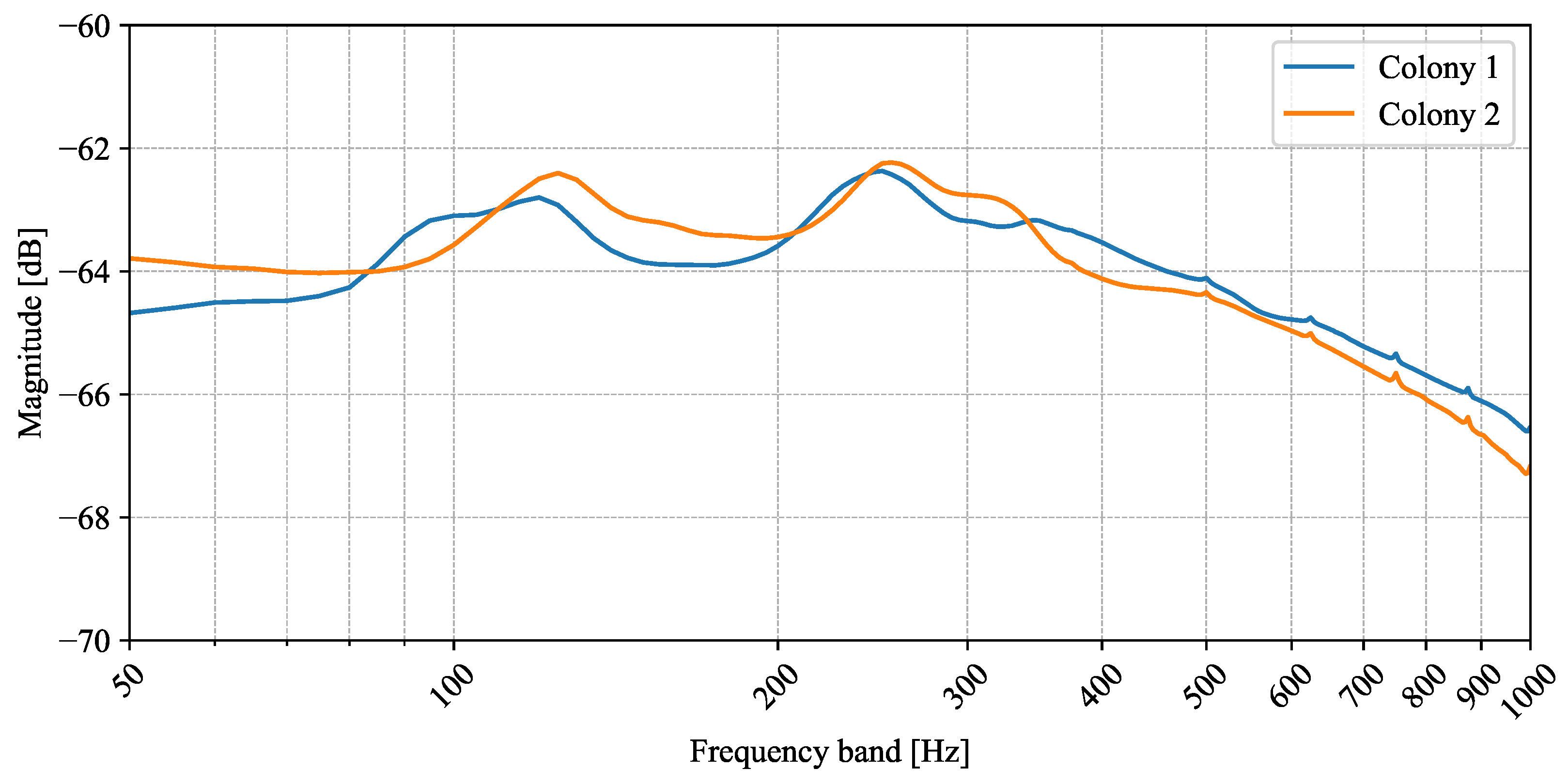
Grouping the vibration spectra according to the colony in which the measurements were recorded showed differences in the recorded spectra over the whole year. In Figure 8 the averaged spectra exhibit different peak frequencies, as well as slightly different amplitudes. Both colonies were recorded with equivalent equipment, belong to the same species and breed and are placed in the same apiary in beehives of the same type. The cause for slight differences in yearly-averaged spectral contents was presumed to be the behavioural patterns of both colonies as well as the relative strength of the colonies.
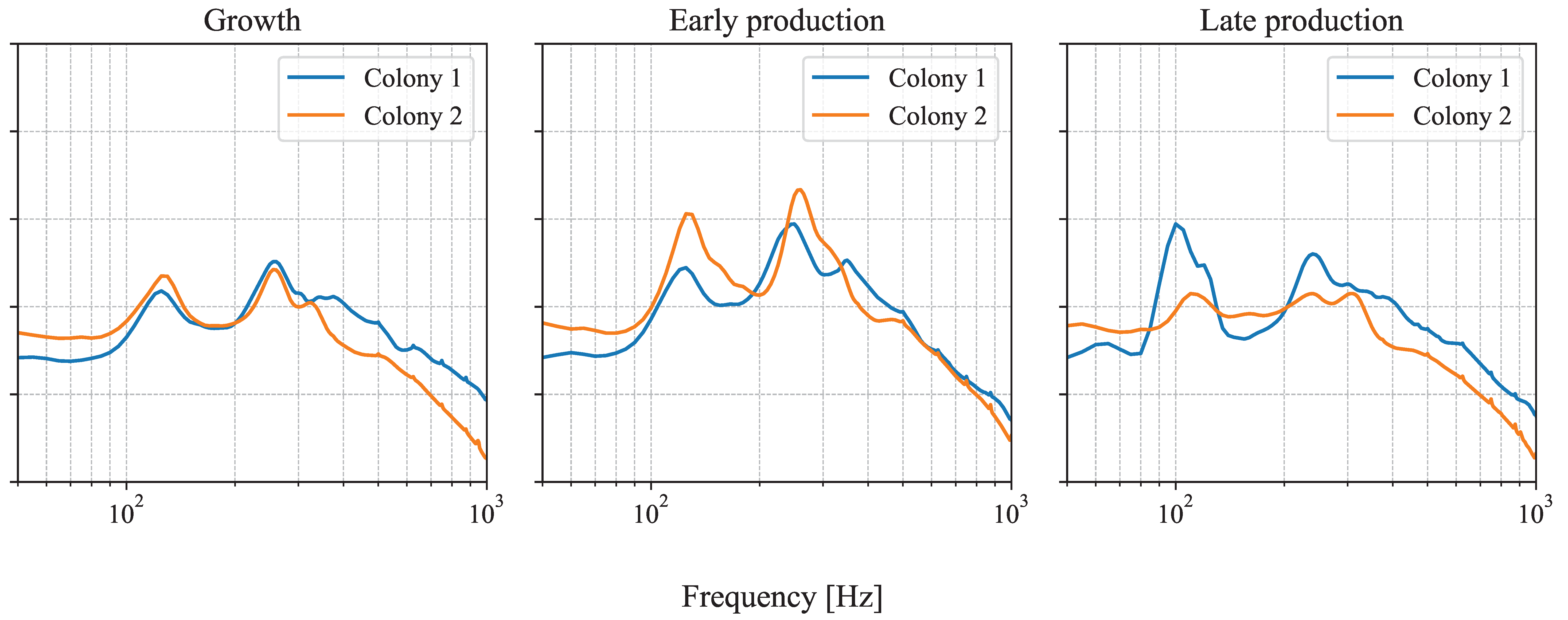
The differences between colonies were not homogenous across all times of year. As seen in Figure 9, the frequency bins align closely during the growth phase, while colony 2 showed heightened activity in the early production phase and colony 1 showed higher amplitudes in the late production phase. As such, the recorded data shows diversity in colony activities, allowing for a more general model than those trained on a single colony.
Once primary testing with the base dataset variant was concluded, a second, filtered dataset was devised. The second dataset was created based on the same principles as the standard one, but with the additional step of introducing a bandpass filter applied before feature extraction occurs. This filtering was introduced as the main energetic bands of the honey bee-produced sound and vibration are below 1 kHz [16]. The filter used was a fifth-order Butterworth filter with the lower cut-off frequency set tp 50 Hz to remove possible structural modes stemming from the hive structure itself. The upper cut-off frequency of the filter was chosen to be 950 Hz in order to introduce attenuation at frequencies approaching 1 kHz without greatly increasing the filter order. The filtered dataset was created to verify whether frequencies at and above 1 kHz impact the accuracy of the classification methods and the frequency bin ranking proposed by the RFECV method.
The data was prepared for machine learning training by first pruning the dataset for non-bee-related outliers (grass cutting, work on beehive structure, and inspections). Then the logarithm of the feature vectors was taken to account for large variance in per-frequency bin energy. Finally, the dataset was split into training and testing subsets, with the testing subset always containing a stratified distribution and accounting for 20% of the whole dataset. The splitting approach did not utilise time-blocking, with purely randomised category samples sorted into training and test sets. This was decided upon as the problem to be solved is classification and the dataset spans one year of measurements, minimising the impact of temporal data leakage on the classifiers. The data was also min-max scaled before passing onto classifiers. The coefficients for min–max scaling were based on the training dataset, so as not to allow any information leakage into the test set.

2.3. Classification Algorithms

Two problems were proposed as part of this experiment. The first and most important one was the classification of the lifecycle period based on the power spectrum of vibrations recorded on top of the brood frames. The secondary task was the identification of the colony based on the same type of data. The guiding principle of this work was to minimise the complexity of chosen classifiers to allow for potential implementation in low-power microcontrollers for future monitoring systems.
Two classification methods were used for the tasks at hand. Multi-Layer Perceptrons (MLPs) were utilised as a high-complexity method resilient to noise as well as local biases in data. Both convolutional neural networks (CNNs) and classical MLPs were used, as both classification tasks required different approaches. The neural networks were implemented using PyTorch 2.8.
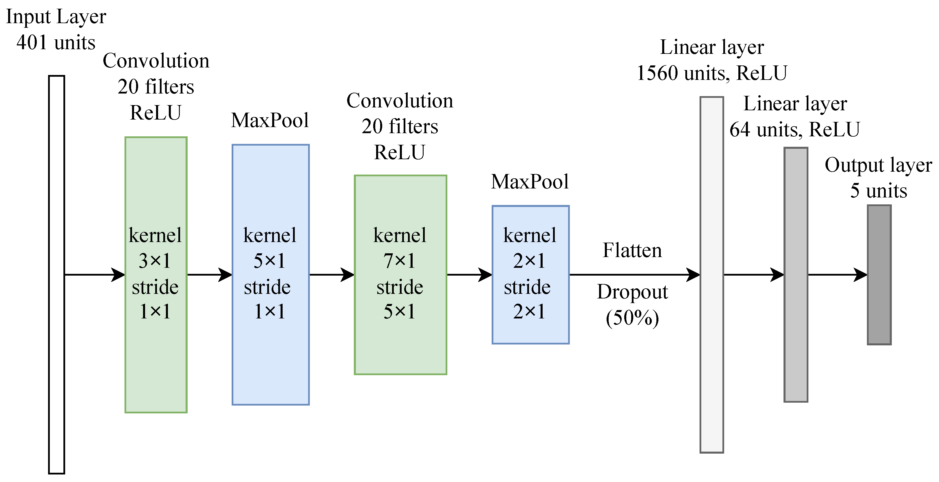
Classification of the lifecycle period was performed by using a CNN, which is shown in Figure 10. The network accepts an input with 401 values and returns an output with 5 values. Within the network architecture there are two one-dimensional convolutional layers with kernels sized at three and seven and strides of one and five. This is followed by two max-pooling layers, one with a five-element kernel and a stride of one, and the second with a two-element kernel and a stride of two. After the convolutional stack, a flattening operation was performed, followed by a 50% dropout and two consecutive linear ReLU-activated layers. The final layer has no activation function, as the cross-entropy loss implementation in PyTorch performs the operation internally. The CNN has 105,949 parameters. The Adam [31] optimizer was used for training with a learning rate of 0.001. The loss function was the weighted cross-entropy loss.
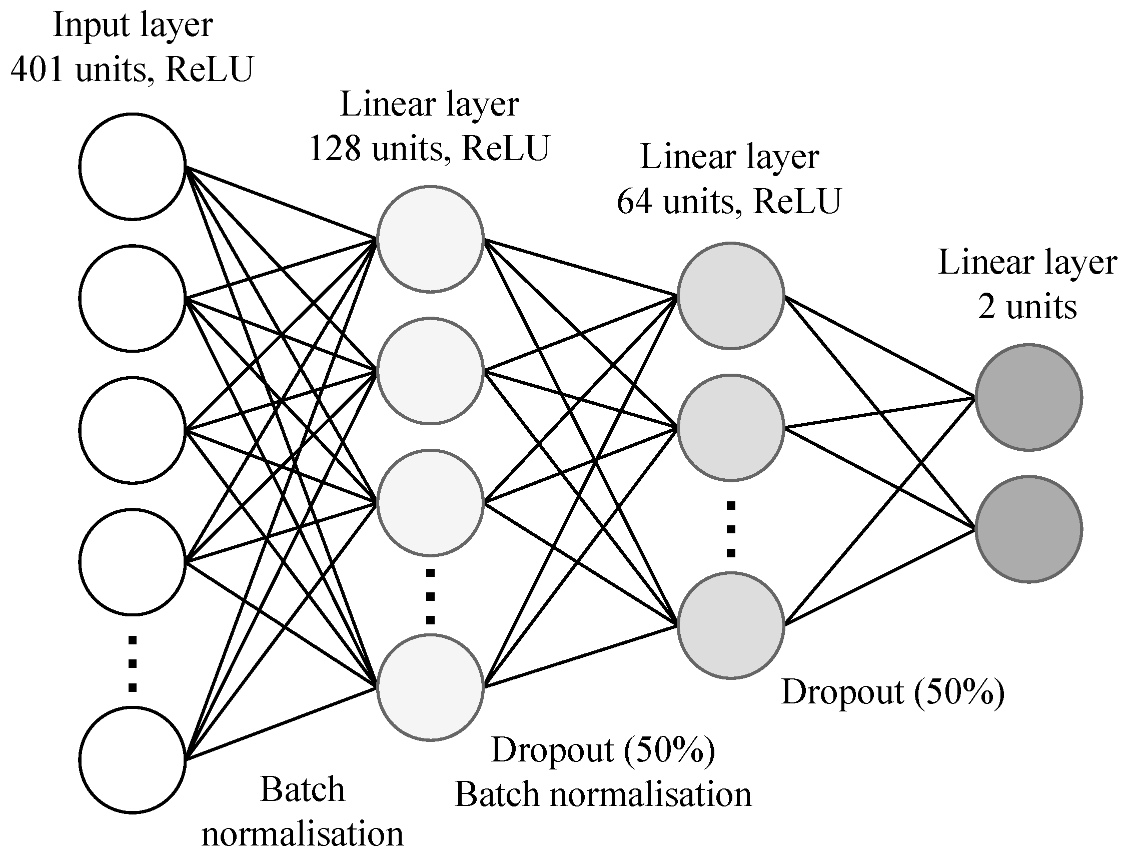
As the secondary task of this work and a possibly much easier problem, the identification of the colony of origin of the recordings utilised a much simpler network. The architecture seen in Figure 11 shows the four overall layers of the network, with the first one being an input layer with 401 neurons. The two following layers are linear ReLU-activated fully connected layers sized at 128 neurons and 64 neurons with batch normalisation and a 50% dropout posed between them and a single batch normalisation before them. The output layer implements two neurons and is preceded by a dropout connection. Similarly to the CNN, the output layer has no activation function. The MLP shows 60,612 trainable parameters. For training, the Adam optimizer was used, with a learning rate of 0.0005; the loss function was the weighted cross-entropy loss.
The batch size for training the networks was 256 feature vectors. All neural networks were trained with an early stopping condition. The networks stopped training if no improvement in the validation score (balanced accuracy) occurred across three epochs.
Besides neural networks, an extra trees (ETs) classifier was utilised to verify the efficacy of the classical machine learning approach. The ET meta estimator was chosen, as the method chosen is typically much faster than random forests for large datasets and uses the whole training dataset instead of bootstrap samples. While similar to random forests, the extra trees approach randomizes feature selection for each split. The ET estimator does not strictly optimize the per-node split, instead calculating the split criterion for a set of random points and choosing the best of them [32].
The classifiers used for the classification of the lifecycle period were ET classifiers with 150 trees. The criterion used for estimating the split quality was Gini impurity and the tree was allowed to grow until there were less than two samples to split. The number of features considered for each split was chosen to be a square root of the overall feature count. For hive origin identification, an identical estimator was used, with the one crucial difference being the maximum depth of the estimator, which was limited to 6 to disallow potential overfitting.
As an additional baseline classification test, logistic regression was also used to verify the basic efficacy of a purely probability-based prediction method for both the primary and secondary task in this work. The logistic regression was optimized using the limited-memory BFGS algorithm with 100 iterations, utilising l2 penalties and optimizing for 500 iterations. Balanced class weighting was used for training and verification of the logistic regression classifier.
All classification algorithms were verified to work on fifteen unique random seed values, with simultaneous re-shuffling of the datasets making for fifteen unique initialisations of the machine learning methods.

2.4. Feature Importance Investigation

To verify which frequency bins are crucial for the tasks at hand, a feature importance investigation was performed using the Recursive Feature Elimination with Cross-Validation method (RFECV) [33]. This approach requires the use of an estimator which is capable of providing an importance for each feature of the dataset. In the case of this work, the ET classifiers were used.
The RFECV method implements multiple Recursive Feature Elimination (RFE) calls. The RFE method provides insight regarding the most important features for a given estimator, based on the iterative elimination of features with the lowest assigned importances. The process is repeated recursively until a model with a set number of features is achieved. This requires the definition of a numbers of features to select, which is a limitation of the pure RFE method.
RFECV uses the RFE method on iteratively smaller feature counts for a given number of cross-validation folds, providing a dataset-averaged scoring for the features. The method then allows for the selection of an optimal number of features which lead to the highest cross-validation averaged score as well as a ranking of features, with the estimated best features assigned rank 1 and higher ranks representing decreasing relevance for the estimator.
It is important to note that, while RFECV can be used on data with correlated input parameters, the method does not guarantee that all rank 1 parameters will be non-correlated. This is an acceptable and even beneficial characteristic for the purposes of this work as the data we are analysing are human-readable and interpretable parameters and correlations between parameters can be inferred from the nature of the vibration source being tested (the presence of more harmonic signals). The RFECV method does not transform the features in any way, but simply simultaneously computes the best features and the features to be chosen, making it a good fit for utilisation with spectral data.

3. Results

The primary results achieved by logistic regression, as the most basic machine learning method, are presented in Table 2. Such base results suggest that the baseline for improvements for more complex classifiers is a balanced accuracy of 82.9% for the determination of lifecycle period using a filtered dataset and 85.6% for non-filtered data. In the case of colony identification, the baseline is 97.8% for the unfiltered case and 97.2% for the filtered case. A near-perfect logistic regression score, combined with very low variance in results across multiple initialisations with multiple random seeds may imply a trivial relationship between the spectral data and the colony in which it was recorded.
The classifiers were trained and their efficacy was evaluated using balanced accuracy as well as the weighted F1 score for lifecycle period classification. Table 3 shows the results of basic classifier verification for both the ET- and CNN-based classifiers and both dataset variants. It can be seen that, for the task of lifecycle period recognition, both methods achieved accuracy scores well over 90%, with the CNN showing a higher score at over 96%. It can also be seen that filtering the dataset did not decrease the efficacy of the tested methods. The mean CNN training epoch number was 74.6 for the standard dataset and 80.6 for the filtered set.
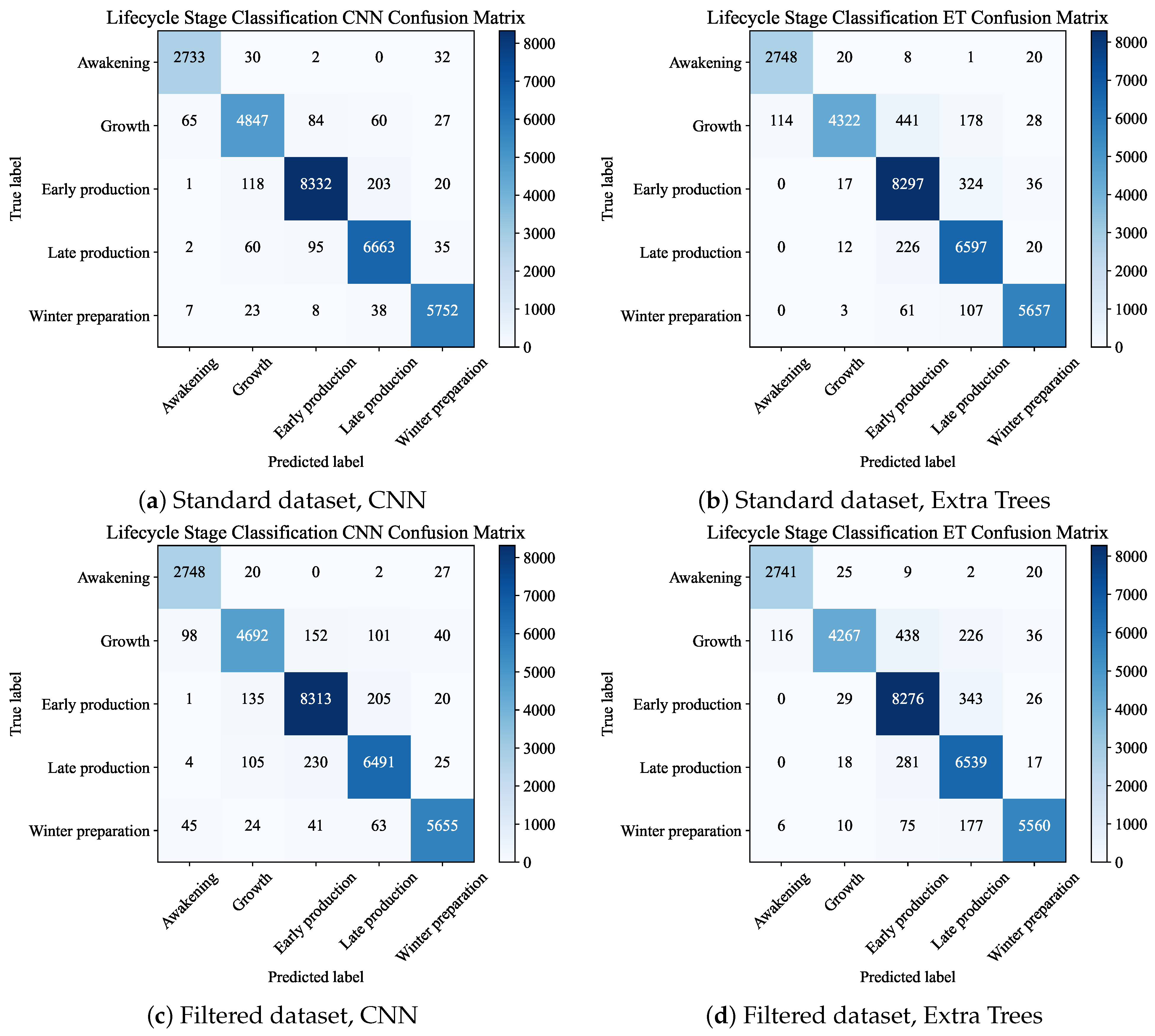
Figure 12 provides deeper insight into the classification, as it shows the confusion matrices for both the CNN and ET models for both dataset variants. While multiple samples from the dataset were misclassified, the overall confusion matrices are largely diagonal with the greatest mistakes occurring in the case of ET models when differentiating between the growth and both production stages, namely early and late production. In the case of both methods, the greatest number of errors can be seen between neighbouring categories, which is most likely caused by the arbitrary nature of the imposed classification.
Table 4 shows the mean accuracies calculated from all fifteen initialisations of the models, divided per category. The accuracy remains mostly consistent through the categories with variations of no more than 5%. The lowest accuracy for all categories in every case is shown by the growth time period. The growth period also shows the greatest standard deviation in accuracy of all categories. As the confusion matrices in Figure 12 show, the growth stage is most commonly confused with the early production stage. As the transition between the growth, early and late production stages is decided by complex combinations of factors, this error may be caused by label noise introduced by the time-based class divisions.
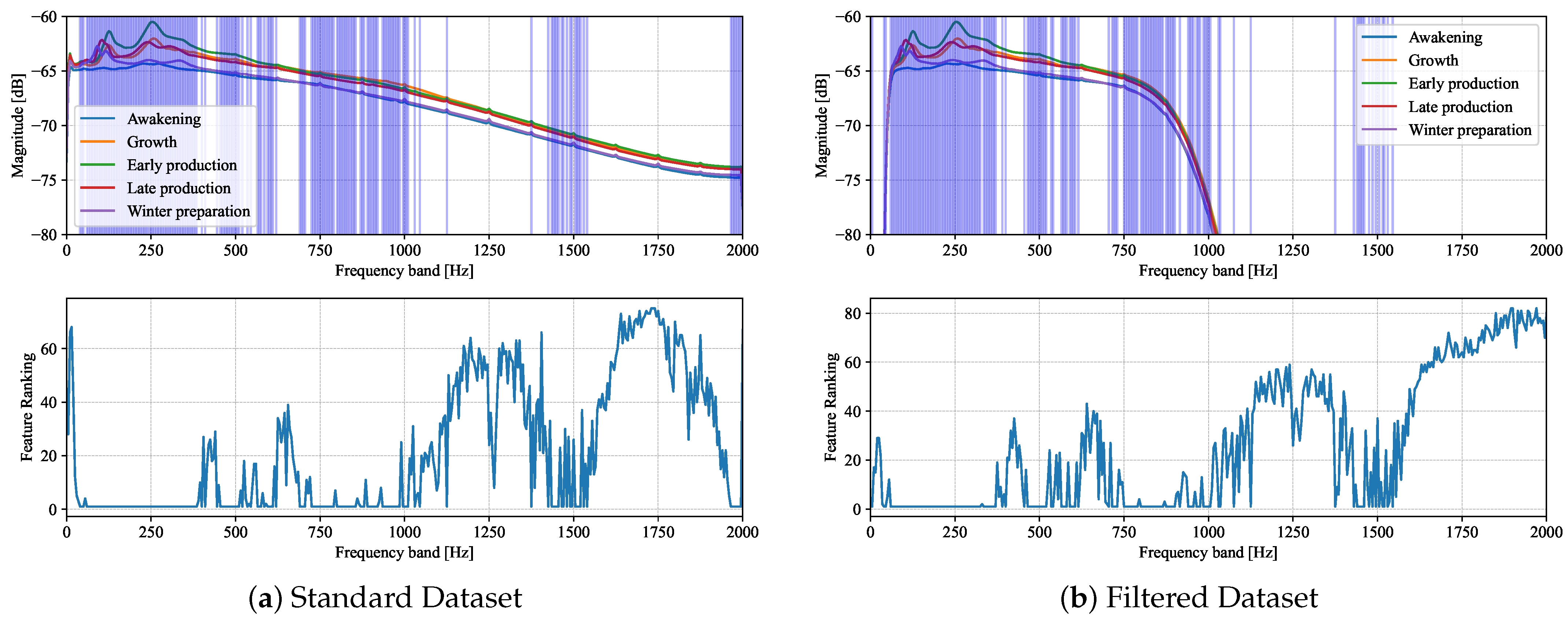
The results shown in Figure 13 show the rankings of each parameter (frequency bin) with higher rankings signifying a lesser importance for the classifier. Both the standard and filtered dataset variants show low rankings in low-frequency bins up to around 300 Hz, with additional low rank regions around 500 Hz as well as between 750 and 1000 Hz. For frequencies higher than 1 kHz the rank rises with only select frequency bins showing dips, specifically at around 1.5 kHz. The filtered dataset shows similar behaviour to the standard one, including the low rank of select frequency bins around 1.5 kHz, showing a repeatable study across both datasets and confirming the cluster of high frequencies with low ranks stem from correlation with lower frequency components.
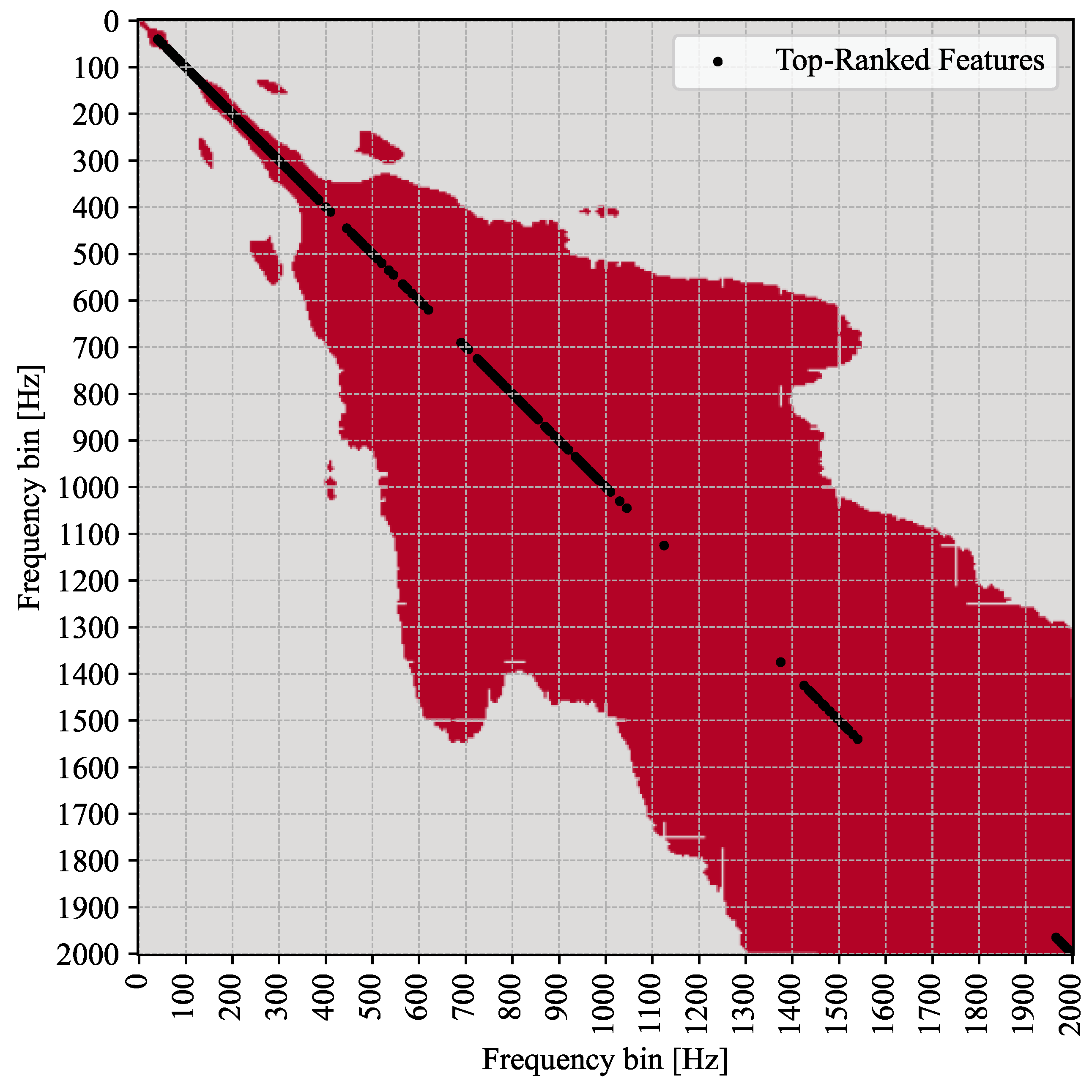
Figure 14 shows a matrix of highly correlated features with frequency bins exhibiting a Pearson correlation coefficient greater or equal to 0.8 (highlighted in red). On the diagonal, dots highlight the rank 1 frequencies from the RFECV analysis. This was necessary, as nearly all components of the vector show at least mild correlation. In the figure, it can be seen that only clearly neighbouring components show high correlations up to around 350 Hz, where a wider range of components is included. It is important to note the harmonic signal frequencies showing correlation in the neighbourhood of 150 Hz bins, with a hotspot at around 300 Hz. A similar case can be seen for the 250 Hz component. The highly correlated neighbourhood increases with frequency and the cluster of recommended frequencies around 1500 Hz is explained as a multiple of the 600 to 800 Hz bins, to which it is highly correlated. This fuels the suspicion that higher frequency bins are not strictly necessary for the task of bee colony lifecycle period estimation.
Table 5 shows the results achieved for the task of colony identification. As can be seen, the scores are near-perfect even with simplified models. This is indicative of trivial relationships within the data such as the modal characteristics of the beehive structure or the noise profile of individual sensors. The MLPs trained in this task for a mean of 22.5 epochs in the case of the standard dataset and 24.7 epochs for the filtered set.
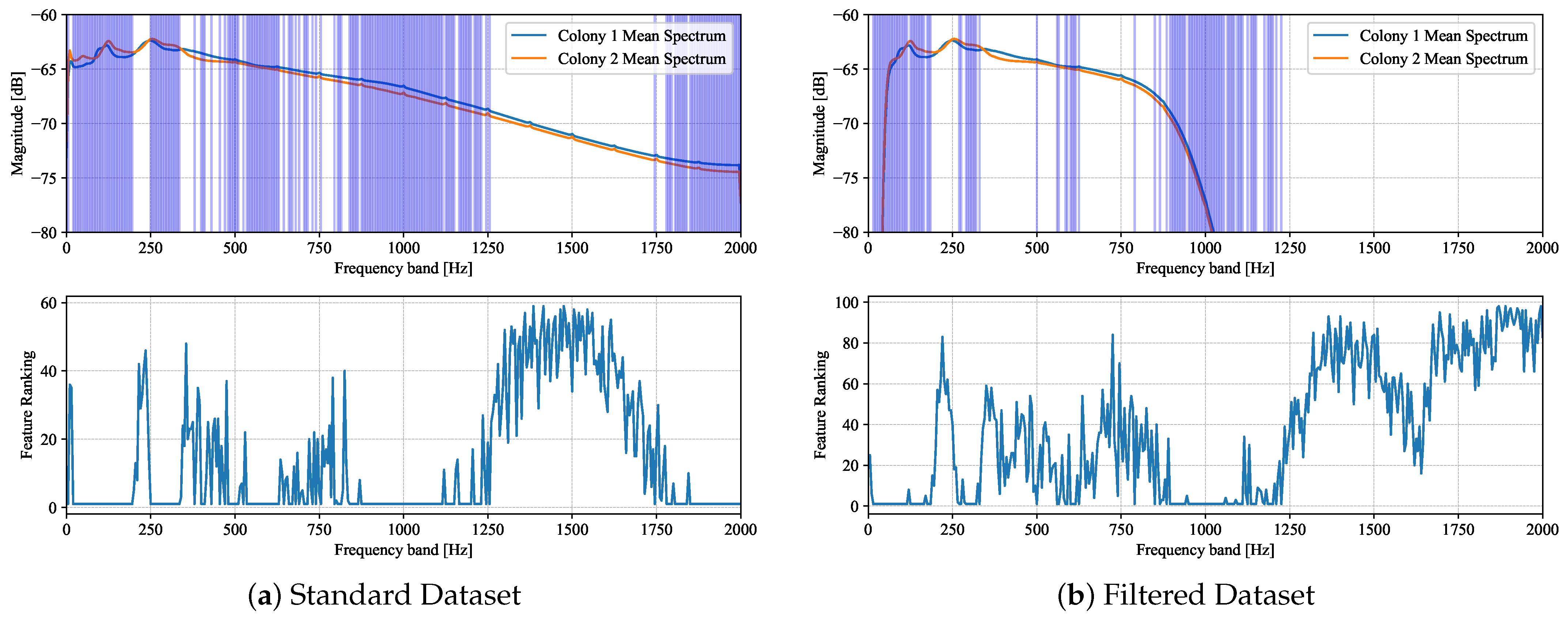
The RFECV analysis, seen in Figure 15, shows that unlike the case of lifecycle period classification, the frequencies chosen for the best-performing models are not clustered in lower frequency bins. A large amount of frequencies around 1750 to 2000 Hz can be seen as important in the standard dataset variant. Filtering the dataset lowers the rank of these frequencies, making them irrelevant for the classifier. In the filtered case, however, it can be seen that lowest-ranked frequencies are positioned around the cut-off frequencies of the filter implying that the ET classifier is learning non-honey bee-related parameters for the identification of colonies, such as the modal characteristics of the beehive itself.
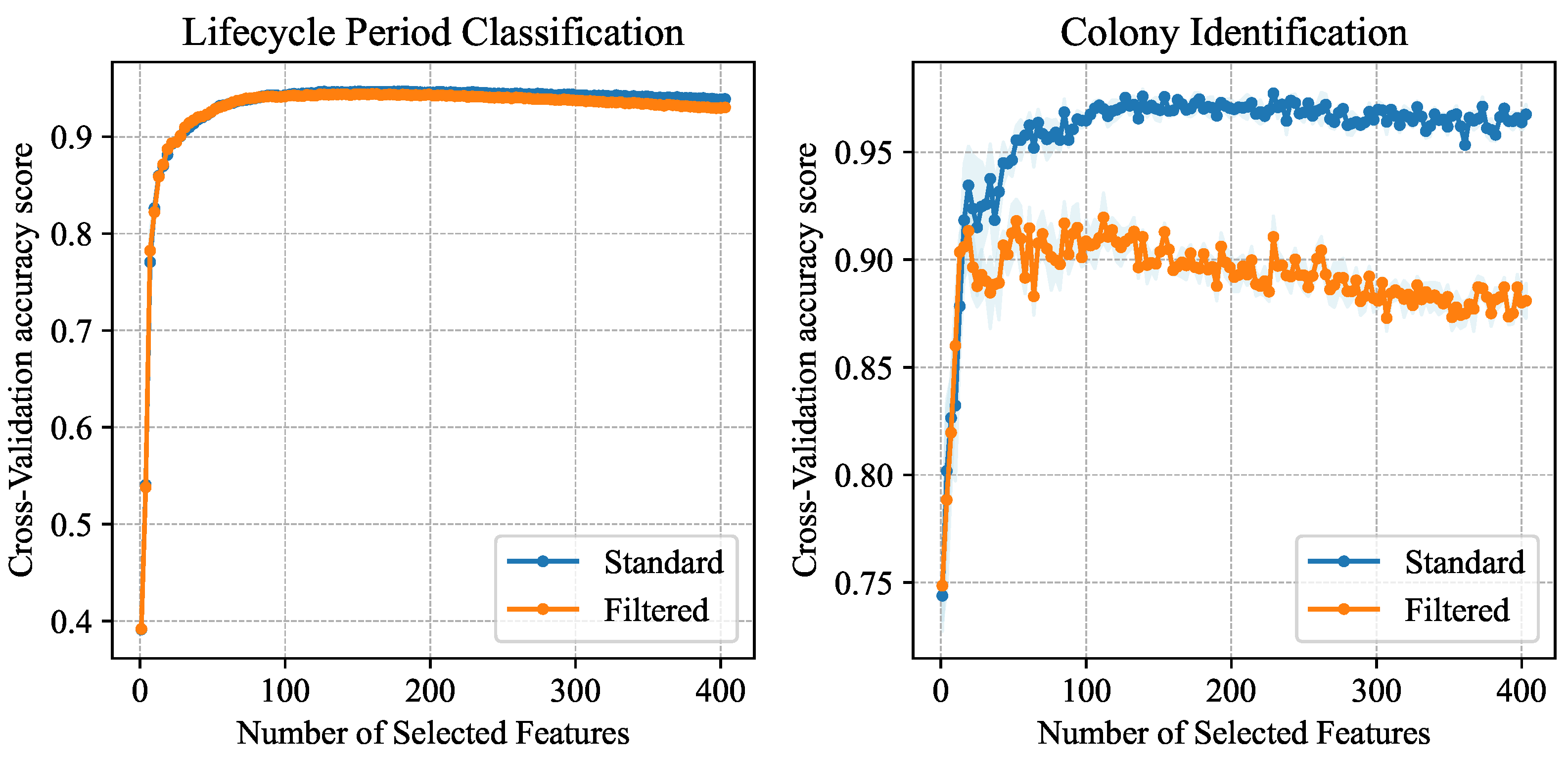
Figure 16 shows the impact of feature count on classifier accuracy. It should be noted that in this graph, unbalanced accuracy was used as the cross-validation score, leading to higher than expected results from the full-dataset study. It can be seen that the lifecycle period classification requires less than 100 features to achieve high accuracy both in the case of the filtered and standard dataset variants. Colony identification meanwhile shows greater variance, reaches a peak score at around 100 features and shows a drastic decline in accuracy when using the filtered dataset. This indicates the colony identification model is training at least partially on noise data and should not be used for diagnostic purposes.

4. Discussion

The results of this study show that recognition of the lifecycle period of honey bee colonies using the vibration signals collected on top of beehive frames is possible both for full-spectrum signals sampled at 4 kHz with spectral information up to 2 kHz and for signals filtered with a passband below 1 kHz. While both CNNs and ET models achieved accuracy scores above 90%, higher than the baseline logistic regression, convolutional networks showed higher scores using both the standard and filtered datasets and reaching a peak accuracy of 97% using the standard dataset. The difference in the balanced accuracies between the filtered and standard dataset results are similar for both neural and classical methods, with both showing a decrease of around 1 percentage point when using filtered data. Such a decrease in efficacy can be expected when nearly half of the input parameters are made insignificant, but the relatively small change in both accuracy and F1 score signifies that the most important frequencies are preserved when bandpass filtering the signals before feature extraction.
The greatest classification errors occurred between neighbouring time categories, with the lowest per-category accuracy occurring in identification of the growth stage. This may indicate that the five-category system devised in this work is slightly oversimplified for utilisation in the early seasons of the year, where many changes occur within the colony very rapidly. The verification of such modifications to the problem paradigm may be left to future work.
This conclusion is supported by the RFECV analysis, which showed that for both the standard and filtered datasets, most of the important frequencies for analysis are positioned below 1 kHz, with nearly identical frequencies being chosen in studies on both dataset variants. While some frequency bins show lower ranks (around 1500 Hz) in both analyses, due to the nature of honey bees as vibration sources, we expect harmonic signals with upper harmonics to occur in the measurements, which is the cause for the appearance of such additional frequency bins, correlated with lower frequencies in the feature importance analysis. Similar results have been achieved for sound data in the task of diurnal pattern recognition [34] and the frequencies most important to classification align with those produced by bee colonies [14,30]. Though no attempt at specific event identification has been made, a conclusion can be drawn that the vibration recorded on top of bee frames used for this work mainly contains frequencies connected to the fundamental frequencies of bee thoraxes [13] and the static wing beat frequency of the colony. It is important to also note the relationship between feature count and the accuracy score achieved by the model in RFECV, which shows that after introducing only around 100 frequency bins, the model reaches over 90% accuracy.
The approach used in this work takes into account the typical use case of a potential bee colony monitoring system with the queens being replaced during the apicultural cycle. While queen replacement may be considered an anomaly in many experiments, in the case of this work, the replacement is a part of the natural yearly colony lifecycle and should be considered as such. The analysis performed also did not utilise any means of time-blocking data splits, typically used with time series data. This poses a risk of inflating the accuracy of the models at the cost of the generalisation toward unseen data. While the risk exists, steps were taken to minimise it by verifying the dataset on multiple random seed initialisations and further verifying the efficacy on a per-time-category basis.
When it comes to the side task of this experiment, that is, the identification of hive origin, the experiment demonstrates that great care needs to be taken when approaching such problems. While spectral differences between the colonies have been shown in the pre-study verification of fundamental frequency distributions, both the neural networks and ET estimators show very high accuracy metrics, reaching a balanced accuracy up to 99.9% in the case of the standard dataset with the MLP classifier. Logistic regression verification suggests a very simple relationship between the recording location and the spectral components of data recorded in the beehive, showing a score of over 97% for both dataset variants. The RFECV analysis provides insight into the task, as frequencies ranked to be the most important occur both in the typical frequency bins emitted by the bee colonies and outside of that range at both higher and lower frequencies. The score is also more variable across feature counts, showing a clear decreasing trend after 100 features in the case of the filtered signal. The model’s behaviour points to the conclusion that trivial relationships may exist between the categories and recorded data—specifically non-bee data. Such relationship stem from the modal characteristics of the beehives in which measurements were performed, sensor noise profiles and the exact positions at which sensors were placed. These relationships are preserved even despite per-sample min–max scaling.
While no directly parallel works based on vibration data have been produced to date, diurnal pattern recognition has been tried using sound data with convolutional neural networks [35]. The results of this study are on par with those found in the literature for such tasks and show not only that the recognition of daily behavioural patterns in bees is possible, but that recognition of yearlong patterns using similar frequency bins can be performed as well [34]. Recognition of the lifecycle period, performed purely on the basis of vibration data, also shows that tasks pertaining to the recognition of honey bee temporal patterns can be performed without the need for amicrophone use inside the hive structure itself, and thus circumventing problems with propolization and wax build-up on sensors placed in bee-accessible spaces.

5. Conclusions

This work has shown that low-cost monitoring of honey bee colonies using accelerometers placed on top of beehive brood frames is a feasible way to achieve completely non-invasive apicultural automation. The signals emitted by bees are informative and the patterns exhibited by the honey bee colony differ with time of year. Machine learning techniques, both classical ET estimators and neural networks represented by CNNs and MLPs, have shown balanced accuracies over 90% when it comes to recognizing the lifecycle period based on the recorded vibration spectra. Filtering the dataset to a sub-1 kHz passband causes relatively small decreases in the model’s efficacy of around one percentage point both for balanced accuracy and F1 scores.
A feature importance study was conducted using the RFECV method, showing that power spectral data in frequency bins up to 1000 Hz are the most important features for the recognition of the lifecycle period of the honey bee colony. The study also shows that around 100 frequency bins is sufficient for this task. The investigation into the determination of the hive of origin indicates that the model for this type of problem is not trained purely on frequency bins connected with honey bees, as filtering the signals decreases the efficacy of the extra trees model drastically, and the feature count investigation found that there is a sharp decline with a rising number of features. This highlights a necessity for future investigations into the differences between bee colonies (ex. breed recognition) based on larger datasets of vibration data differing in terms of hive construction, hardware used and apiary location. The data used for such tasks needs to be diverse in terms of the location of measurement devices, hive types and sensors used to allow for more general models to be developed.
The results of this study show that the most informative frequency bins for the recognition of honey bee lifecycle periods are situated under 1 kHz. Models trained on filtered signals have shown negative, but overall small deviations from the standard datasets. This leads to the conclusion that decreasing the sampling rate of the accelerometer to 2 kHz for future monitoring works may be performed as a compromise, to limit the large data storage requirements of future datasets. This conclusion may be validated in future work by testing on various tasks such as swarming detection and queen bee presence detection to provide more robust confirmation.
The results achieved in this work, while significant, are a proof of concept. The conclusions are constrained by the bounds of plausible generalisation, which is limited by the following factors:
1.
The dataset used for verification, both in terms of maintenance-caused discontinuities and the low sample size;
2.
Data sourced from only a single bee breed within a single apiary;
3.
Possible label noise introduced by hard limits on classification categorisation;
4.
A single year of measurements, necessitating the use of non-time blocking dataset split techniques, possibly inflating results due to correlations between training and testing data.
Making the conclusions of this manuscript more generalisable is a direction for future work, as based on the findings more and larger datasets with an improved version of the monitoring set-up in multiple apiaries over many apicultural seasons will be created. With multiple years of comparable measurements available, cross-season verification can be used for truly time correlation-independent verification of the utilised methods. With more data, a robust label sensitivity study can also be performed. In the end, a general model of the honey bee colony yearly lifecycle may be proposed, based on such diverse and robust bee vibration datasets, which will allow for the development of an IoT lifecycle monitoring apicultural assistant.

Author Contributions

Conceptualization, P.K. and B.S.; methodology, P.K., B.S. and A.R.; software, P.K.; validation, P.K., B.S. and A.R.; formal analysis, P.K.; investigation, P.K.; resources, P.K., B.S. and A.R.; data curation, P.K.; writing—original draft preparation, P.K. and A.R.; writing—review and editing, P.K., B.S. and A.R.; visualization, P.K.; supervision, B.S.; project administration, B.S.; funding acquisition, B.S. All authors have read and agreed to the published version of the manuscript.

Funding

This research received no external funding.

Institutional Review Board Statement

Not applicable.

Informed Consent Statement

Not applicable.

Data Availability Statement

Experiment data will be made available upon reasonable request to the authors. The code used for neural network training is available publicly at https://github.com/L0ranos/Vibration_bees_Applsci_2025 (accessed on 22 December 2025).

Conflicts of Interest

The authors declare no conflicts of interest.

Abbreviations

The following abbreviations are used in this manuscript:
CNNConvolutional Neural Network
MLPMulti-Layer Perceptron
ETExtra Trees
CVCross-Validation
RFECVRecursive Feature Elimination with Cross-Validation

Appendix A

Honey bees are animals heavily influenced by environmental factors, chief of which could be the weather in the vicinity of the apiary in which the bees reside. While meteorological monitoring was not performed through the duration of the experiment within the selected apiary, data on the mean temperature and total rainfall around the location of the colonies is available from the Open-Meteo collection [36].
The mean daily temperature at two metres above ground level and the total rainfall for the location of the apiary were downloaded from the repository and are shown in Figure A1. Overall, the measured dataset contains a diverse spread of temperatures as well as precipitation conditions, which was expected for long-term measurements.
Figure A1. Meteorological data around the selected apiary as per data available from Open-Meteo. The four significant outage periods are highlighted in gray.
Applsci 16 00188 g0a1
The weather patterns during the measurement outages in most cases reflect the meteorological conditions present during other periods. The last and first measurement gap, however, differ from this noticeably, showing a drastic increase in temperatures above 15 °C in the April gap and a decrease in temperature below 10 °C. Both of these periods would show great changes in colony behaviour and would represent a transient state. The lack of measurements at these times is unfortunate; however, measurements are present both at the start and at the end of these periods, only lacking data in the transitions. As such, it seems that many states of the colonies have been recorded, and the dataset can be considered valid for the purposes of the proof-of-concept method and feature importance analysis. It is crucial to highlight the importance of continuity of measurement in future monitoring endeavours, including the gathering of environmental parameters such as temperature and precipitation.

References

  1. Jeong, K.; Oh, H.; Lee, Y.; Seo, H.; Jo, G.; Jeong, J.; Park, G.; Choi, J.; Seo, Y.D.; Jeong, J.H.; et al. IoT and AI Systems for Enhancing Bee Colony Strength in Precision Beekeeping: A Survey and Future Research Directions. IEEE Internet Things J. 2025, 12, 362–389. [Google Scholar] [CrossRef]
  2. Szczurek, A.; Maciejewska, M.; Batog, P. Monitoring System Enhancing the Potential of Urban Beekeeping. Appl. Sci. 2023, 13, 597. [Google Scholar] [CrossRef]
  3. Verbeke, W.; Diallo, M.A.; van Dooremalen, C.; Schoonman, M.; Williams, J.H.; Van Espen, M.; D’Haese, M.; de Graaf, D.C. European beekeepers’ interest in digital monitoring technology adoption for improved beehive management. Comput. Electron. Agric. 2024, 227, 109556. [Google Scholar] [CrossRef]
  4. Karmańska, A.; Ziemba, E.W.; Maruszewska, E.W.; Jarka, S. Socio-Demographic Factors Influencing Adoption of Digital Technologies in Beekeeping. J. Apic. Sci. 2025, 69, 29–41. [Google Scholar] [CrossRef]
  5. Turyagyenda, A.; Katumba, A.; Akol, R.; Nsabagwa, M.; Mkiramweni, M.E. IoT and Machine Learning Techniques for Precision Beekeeping: A Review. AI 2025, 6, 26. [Google Scholar] [CrossRef]
  6. Dsouza, A.; P, A.; Hegde, S. HiveLink, an IoT based Smart Bee Hive Monitoring System. arXiv 2023, arXiv:2309.12054. [Google Scholar]
  7. Meikle, W.G.; Rector, B.G.; Mercadier, G.; Holst, N. Within-day variation in continuous hive weight data as a measure of honey bee colony activity. Apidologie 2008, 39, 694–707. [Google Scholar] [CrossRef]
  8. Bjerge, K.; Frigaard, C.E.; Mikkelsen, P.H.; Nielsen, T.H.; Misbih, M.; Kryger, P. A computer vision system to monitor the infestation level of Varroa destructor in a honeybee colony. Comput. Electron. Agric. 2019, 164, 104898. [Google Scholar] [CrossRef]
  9. Dreller, C.; Kirchner, W. Hearing in honeybees: Localization of the auditory sense organ. J. Comp. Physiol. A 1993, 173, 275–279. [Google Scholar] [CrossRef]
  10. Kirchner, W. Hearing in honeybees: The mechanical response of the bee’s antenna to near field sound. J. Comp. Physiol. A 1994, 175, 261–265. [Google Scholar] [CrossRef]
  11. Michelsen, A.; Kirchner, W.H.; Lindauer, M. Sound and vibrational signals in the dance language of the honeybee, Apis mellifera. Behav. Ecol. Sociobiol. 1986, 18, 207–212. [Google Scholar] [CrossRef]
  12. Hrncir, M.; Maia-Silva, C.; Farina, W.M. Honey bee workers generate low-frequency vibrations that are reliable indicators of their activity level. J. Comp. Physiol. A Neuroethol. Sens. Neural Behav. Physiol. 2019, 205, 79–86. [Google Scholar] [CrossRef] [PubMed]
  13. Jankauski, M.A. Measuring the frequency response of the honeybee thorax. Bioinspiration Biomimetics 2020, 15, 046002. [Google Scholar] [CrossRef]
  14. Ramsey, M.; Bencsik, M.; Newton, M.I. Long-term trends in the honeybee whooping signal’ revealed by automated detection. PLoS ONE 2017, 12, e0181736. [Google Scholar] [CrossRef]
  15. Ramsey, M.T.; Bencsik, M.; Newton, M.; Reyes Carreño, M.; Pioz, M.; Crauser, D.; Simon-Delso, N.; Le Conte, Y. The prediction of swarming in honeybee colonies using vibrational spectra. Sci. Rep. 2020, 10, 9798. [Google Scholar] [CrossRef]
  16. Ramsey, M.; Bencsik, M.; Newton, M. Extensive Vibrational Characterisation and Long-Term Monitoring of Honeybee Dorso-Ventral Abdominal Vibration signals. Sci. Rep. 2018, 8, 14571. [Google Scholar] [CrossRef]
  17. Cejrowski, T.; Szymański, J.; Mora, H.; Gil, D. Detection of the Bee Queen Presence Using Sound Analysis. In Intelligent Information and Database Systems; Springer International Publishing: Berlin/Heidelberg, Germany, 2018; pp. 297–306. [Google Scholar] [CrossRef]
  18. De Simone, A.; Barbisan, L.; Turvani, G.; Riente, F. Advancing Beekeeping: IoT and TinyML for Queen Bee Monitoring Using Audio Signals. IEEE Trans. Instrum. Meas. 2024, 73, 2527309. [Google Scholar] [CrossRef]
  19. Zgank, A. Bee Swarm Activity Acoustic Classification for an IoT-Based Farm Service. Sensors 2020, 20, 21. [Google Scholar] [CrossRef]
  20. Iqbal, K.; Alabdullah, B.; Al Mudawi, N.; Algarni, A.; Jalal, A.; Park, J. Empirical Analysis of Honeybees Acoustics as Biosensors Signals for Swarm Prediction in Beehives. IEEE Access 2024, 12, 148405–148421. [Google Scholar] [CrossRef]
  21. Kulyukin, V.; Mukherjee, S.; Amlathe, P. Toward Audio Beehive Monitoring: Deep Learning vs. Standard Machine Learning in Classifying Beehive Audio Samples. Appl. Sci. 2018, 8, 1573. [Google Scholar] [CrossRef]
  22. Libal, U.; Biernacki, P. Non-Intrusive System for Honeybee Recognition Based on Audio Signals and Maximum Likelihood Classification by Autoencoder. Sensors 2024, 24, 5389. [Google Scholar] [CrossRef]
  23. Mezquida Atauri, D.; Llorente Martínez, J. Platform for bee-hives monitoring based on sound analysis. A perpetual warehouse for swarm’s daily activity. Span. J. Agric. Res. 2009, 7, 824–828. [Google Scholar] [CrossRef]
  24. Uthoff, C.; Homsi, M.N.; von Bergen, M. Acoustic and vibration monitoring of honeybee colonies for beekeeping-relevant aspects of presence of queen bee and swarming. Comput. Electron. Agric. 2023, 205, 107589. [Google Scholar] [CrossRef]
  25. Šabić, J.; Perković, T.; Šolić, P.; Šerić, L. Buzzing with Intelligence: A Systematic Review of Smart Beehive Technologies. Sensors 2025, 25, 5359. [Google Scholar] [CrossRef]
  26. Döke, M.A.; Frazier, M.; Grozinger, C.M. Overwintering honey bees: Biology and management. Curr. Opin. Insect Sci. 2015, 10, 185–193. [Google Scholar] [CrossRef]
  27. Winston, M.L. The Biology of the Honey Bee; Harvard University Press: London, UK, 1991. [Google Scholar]
  28. Rahman, M.; Saifur Rahman, M.; Parvin, N.; Rahman, M. Fundamental Frequency Extraction by Utilizing the Modified Weighted Autocorrelation Function in Noisy Speech. Lect. Notes Netw. Syst. 2024, 890, 65–76. [Google Scholar] [CrossRef]
  29. Welch, P. The use of fast Fourier transform for the estimation of power spectra: A method based on time averaging over short, modified periodograms. IEEE Trans. Audio Electroacoust. 1967, 15, 70–73. [Google Scholar] [CrossRef]
  30. Ksiazek, P.; Libal, U. Impact of Time of Day on Spectral and Entropic Parameters of Honeybee Audio Signals. In Proceedings of the 2025 Signal Processing Symposium (SPSympo), Warsaw, Poland, 8–10 July 2025; pp. 84–89. [Google Scholar] [CrossRef]
  31. Kingma, D.P.; Ba, J. Adam: A Method for Stochastic Optimization. arXiv 2014, arXiv:1412.6980. [Google Scholar] [CrossRef]
  32. Geurts, P.; Ernst, D.; Wehenkel, L. Extremely Randomized Trees. Mach. Learn. 2006, 63, 3–42. [Google Scholar] [CrossRef]
  33. Awad, M.; Fraihat, S. Recursive Feature Elimination with Cross-Validation with Decision Tree: Feature Selection Method for Machine Learning-Based Intrusion Detection Systems. J. Sens. Actuator Netw. 2023, 12, 67. [Google Scholar] [CrossRef]
  34. Książek, P.; Libal, U.; Król-Nowak, A. Spectral Components of Honey Bee Sound Signals Recorded Inside and Outside the Beehive: An Explainable Machine Learning Approach to Diurnal Pattern Recognition. Sensors 2025, 25, 4424. [Google Scholar] [CrossRef] [PubMed]
  35. Amlathe, P. Standard Machine Learning Techniques in Audio Beehive Monitoring: Classification of Audio Samples with Logistic Regression, K-Nearest Neighbor, Random Forest and Support Vector Machine. Master’s Thesis, Utah State University, Logan, UT, USA, 2018. [Google Scholar]
  36. Zippenfenig, P. Open-Meteo.com Weather API. 2023. Available online: https://zenodo.org/records/14582479 (accessed on 15 December 2025).
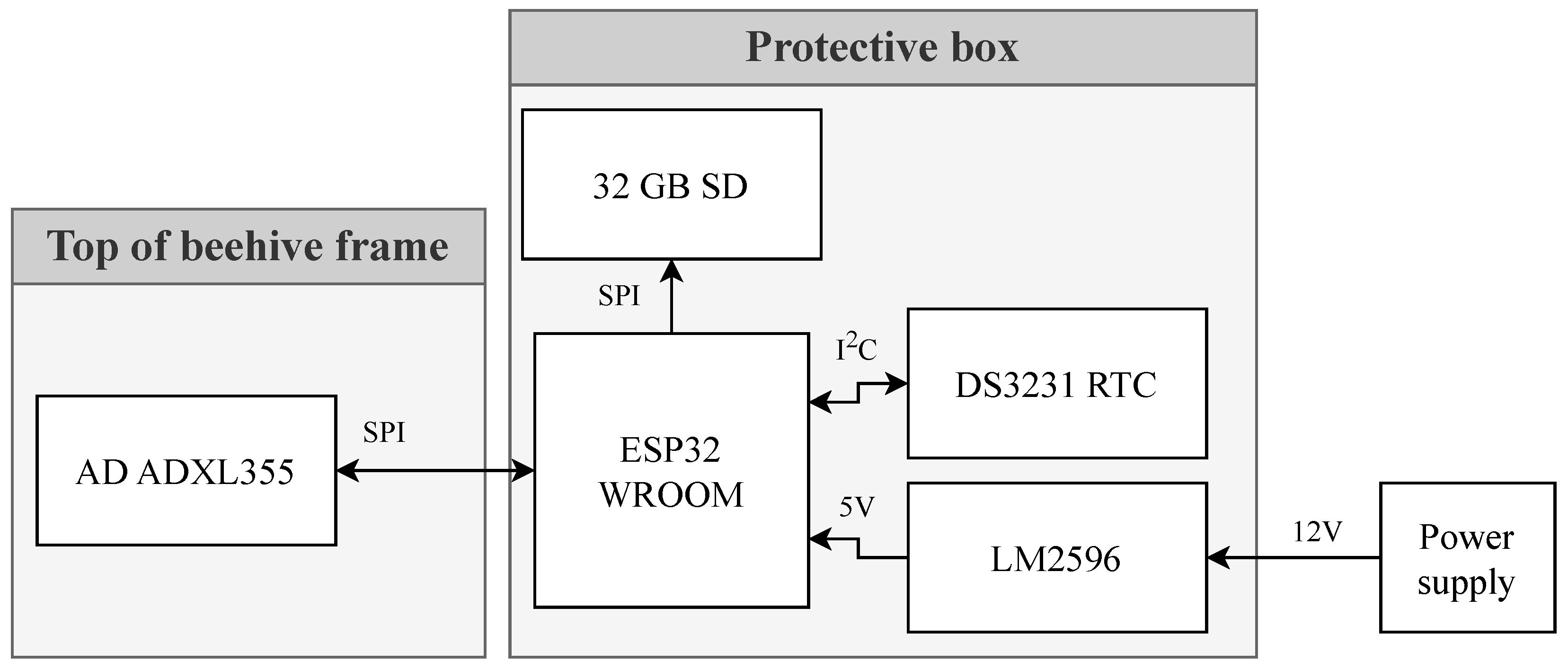
Figure 1. Diagram of measurement station used in the experiment.
Applsci 16 00188 g001
Figure 2. Measurement station placed in Hive 1.
Applsci 16 00188 g002
Figure 3. Lifecycle periods used for the classification throughout the apicultural season. Grey lines signify weeks during which outages occurred affecting both measurement stations within the apiary.
Applsci 16 00188 g003
Figure 4. Forage availability chart in the foraging area of the analysed colonies. Blue blocks represent growth forage (used by the colonies); green blocks represent production forage (gathered as honey by the beekeepers).
Applsci 16 00188 g004
Figure 5. Lifecycle period classification category counts.
Applsci 16 00188 g005
Figure 6. Violin plots of fundamental frequency values in datasets grouped by lifecycle period and colony. Blue distributions belong to colony 1, orange to colony 2. Horizontal lines signify the median value.
Applsci 16 00188 g006
Figure 7. Averaged vibration spectra per colony lifecycle period.
Applsci 16 00188 g007
Figure 8. Vibration spectra averaged over the whole measurement period recorded in both colonies.
Applsci 16 00188 g008
Figure 9. Averaged vibration spectra per lifecycle period and measured colony.
Applsci 16 00188 g009
Figure 10. CNN architecture used for classification of lifecycle period.
Applsci 16 00188 g010
Figure 11. MLP architecture used for classification of hive origin.
Applsci 16 00188 g011
Figure 12. Confusion matrices for lifecycle period classification by CNN and ET models.
Applsci 16 00188 g012
Figure 13. RFECV results of lifecycle period classification for different dataset variants. Blue stripes signify the frequencies supported by analysis.
Applsci 16 00188 g013
Figure 14. Highly correlated features according to Pearson correlation ( r 0.8 ). Standard dataset variant.
Applsci 16 00188 g014
Figure 15. RFECV results of colony identification for different dataset variants. Blue stripes signify the frequencies supported by analysis.
Applsci 16 00188 g015
Figure 16. Graph of mean cross-validation scores of ET models with different feature counts. Shaded areas denote the standard deviation of results for given number of features.
Applsci 16 00188 g016
Table 1. Lifecycle periods established for the purposes of this study based on observations in the measurement apiary.
Class NumberPeriod NameEventsTemporal Bounds
0AwakeningThe queen resumes egg laying, the overwintered brood is reared, the spring flight occurs at the end01.02–01.03
1GrowthStart of foraging, intensive colony growth, drone rearing occurs.01.03–01.05
2Early productionForaging for early nectar and pollen. Peak drone population.01.05–15.07
3Late productionForaging for later nectar and pollen.15.07–15.08
4Winter preparationLate blooming forage. Sugar syrup feeding and Varroa treatments are performed.15.08–25.10
Table 2. Logistic regression primary test results.
TaskDataset VariantMean AccuracyStd Accuracy
Lifecycle period classificationStandard85.6%0.2%
Filtered82.9%0.2%
Colony identificationStandard97.8%0.1%
Filtered97.2%0.1%
Table 3. Model results for identification of lifecycle period.
ModelDataset VariantMean AccuracyStd AccuracyF1 ScoreStd F1 Score
CNNStandard96.7%0.4%96.5%0.3%
Filtered95.9%0.5%95.7%0.5%
ETStandard94.2%0.2%94.1%0.2%
Filtered93.4%0.2%93.3%0.2%
Table 4. Per-class accuracies for lifecycle recognition experiments on multiple random initialisations for both dataset variants.
Standard Dataset
Lifecycle PeriodCNNET
Mean AccuracyStd AccuracyMean AccuracyStd Accuracy
Awakening98.6%0.5%98.3%0.3%
Growth94.0%0.8%84.3%0.6%
Early production95.8%0.5%95.3%0.3%
Late production97.3%0.6%96.2%0.2%
Winter preparation97.9%0.6%96.8%0.2%
Filtered Dataset
Awakening98.2%0.3%98.1%0.3%
Growth93.2%1.1%83.0%0.5%
Early production95.3%0.7%94.9%0.3%
Late production95.6%0.9%95.6%0.3%
Winter preparation97.3%0.8%95.1%0.3%
Table 5. Model results for colony identification.
ModelDataset VariantMean AccuracyStd AccuracyF1 ScoreStd F1 Score
MLPStandard99.8%0.0%99.8%0.0%
Filtered99.6%0.1%99.6%0.1%
ETStandard95.9%0.6%95.8%0.6%
Filtered86.7%0.6%86.3%0.7%
Disclaimer/Publisher’s Note: The statements, opinions and data contained in all publications are solely those of the individual author(s) and contributor(s) and not of MDPI and/or the editor(s). MDPI and/or the editor(s) disclaim responsibility for any injury to people or property resulting from any ideas, methods, instructions or products referred to in the content.