Monitoring Water Area Dynamics in Kashgar (2003–2023) Using Multi-Source Remote Sensing Data

Abstract

Understanding the dynamics of regional water area changes is crucial for effective water resource management and ecological conservation, particularly in arid regions. Located in northwestern China’s arid zone, changes in water area in Kashgar significantly impact local agricultural productivity, ecological integrity, and human socioeconomic activities. However, long-term trends in water area changes and their driving factors in Kashgar remain poorly understood. This study leverages Landsat and Sentinel-2 imagery from 2003 to 2023, employing a random forest algorithm to extract water body information. Key findings are as follows: (1) both total and seasonal water area exhibit a fluctuating downward trend, while permanent water area displays a fluctuating upward trend; (2) precipitation and temperature emerged as primary drivers of water area changes, with precipitation in the surrounding regions of Kashgar exerting a particularly significant influence, while evaporation exhibited a lesser impact; (3) the influence of climate change and anthropogenic activities in surrounding areas on water area changes in Kashgar cannot be overlooked.

1. Introduction

Water resources are fundamental to human survival and socio-economic development, serving as a crucial component of ecosystems [1]. They play a vital role in climate change research, ecological studies, and natural disaster monitoring [2]. Effective monitoring of surface water dynamics is essential for understanding hydrological processes and informing sustainable water resource management [3]. Surface water information extraction provides critical data to support the achievement of the United Nations Sustainable Development Goals (SDGs), specifically those related to ensuring sustainable water management and access [4].

The study of surface water dynamics has traditionally relied on discontinuous time ranges, which can obscure crucial turning points. Utilizing continuous time series remote sensing data to investigate the spatiotemporal evolution of regional surface water bodies is therefore paramount for a comprehensive understanding of hydrological processes and for informing effective water resource management strategies. Recent advancements in remote sensing technology and data processing capabilities have enabled researchers to leverage continuous long-term remote sensing data for surface water change analysis. For instance, Pekel et al. (2016) generated the first global 30-m resolution surface water change product using Landsat imagery on the Google Earth Engine (GEE) platform. By calculating water body frequency, they classified different water body types and quantitatively analyzed global surface water dynamics from 1984 to 2015 [5]. Zou et al. (2018) employed a mixed index rule based on MNDWI, NDVI, and EVI to extract long-term surface water bodies in the United States from 1984 to 2016. They analyzed interannual variations in water area and explored the influence of anthropogenic activities and meteorological factors on water area dynamics [6]. Domestically, numerous studies have also been conducted. Wang et al. (2018) utilized NDWI, NDVI, MNDWI, and a random forest classification method on the GEE platform to rapidly delineate annual maximum and minimum surface water extents in the middle reaches of the Yangtze River from 1990 to 2017 [7]. Deng et al. (2019) developed a multi-index water body detection rule (MIWDR) using MNDWI, AWEI, NDVI, and EVI to efficiently extract long-term surface water bodies in the Yangtze River Basin from 1984 to 2018. They analyzed spatiotemporal variation characteristics and influencing factors [8]. Han et al. (2020) constructed a new global surface water dataset (Global Surface Water Extent Dataset, GSWED) based on the GEE platform, covering the period from 2000 to 2018, and analyzed long-term trends in surface water bodies across different regions [9]. Huang et al. (2021) extracted surface water areas in the Irtysh River Basin using Landsat imagery from 1990 to 2019 and explored the impact of climate change and urbanization on the basin [10]. Furthermore, Li et al. (2022) extracted surface water bodies in the Lake Baikal Basin from 2013 to 2021 using GEE and deep learning models. This approach effectively reduced the time required for manual water body labeling and improved classification accuracy [11]. Olthof et al. (2023) employed Landsat sub-pixel mapping to map surface water bodies in Canada’s Hudson Bay region from 1985 to 2021, calculating surface water area trends across the entire time series [12]. In conclusion, the study of surface water dynamics is transitioning from discontinuous time segment analysis to continuous long-term remote sensing analysis. This shift will provide crucial insights into hydrological processes and support the development of more scientifically informed water resource management strategies.

Surface water area exhibits significant interannual and intra-annual variability. Consequently, delineating water bodies solely based on single remote sensing images introduces considerable uncertainty [13]. This uncertainty stems from two primary factors. First, seasonal fluctuations in water extent make it challenging to capture the full range of annual variability using a single image acquisition. Determining the optimal acquisition time to meet specific research objectives is also problematic as images acquired during the rainy season will reflect maximum water extent, whereas those acquired during the dry season will primarily depict permanent water bodies. To mitigate this uncertainty, utilizing a full-year time series of imagery is recommended. Second, interannual variability in water area can further complicate trend analysis. Even when using images acquired on the same date across multiple years, accurately capturing long-term trends can be difficult, potentially leading to inconsistencies in both water area and the number of water bodies [14]. Accurately determining the temporal position of a single image within a year, as well as the corresponding temporal position of images acquired on the same date in different years, is crucial for minimizing uncertainty. Therefore, a comprehensive understanding of surface water area dynamics necessitates the analysis of a substantial dataset of remote sensing imagery spanning multiple seasons and years.

Rivers and lakes, as vital regional water resources, exhibit high sensitivity to climate change in the Kashgar region. These key geomorphic units play a crucial role in mitigating the impacts of global warming on the region [15]. However, persistent water scarcity has consistently constrained economic and social development in Kashgar, leading to ecosystem fragility [16]. Population growth and economic development have further exacerbated this water shortage issue [17]. Against the backdrop of global warming, changes in water bodies in Kashgar directly reflect the dynamic trends of regional water resources. Despite the scarcity of long-term studies on water body dynamics in the Kashgar region, accurate quantification of water body area and an understanding of their spatiotemporal variations are crucial. This information is essential for ensuring the sustainable development of the local economy and society, as well as for safeguarding the ecological environment.

Given the significance of water resources in the arid region of Kashgar, understanding their spatiotemporal dynamics and the influence of climate change is crucial for predicting future water availability and developing sustainable management strategies. This study leverages the Google Earth Engine (GEE) platform, Landsat and Sentinel-2 satellite imagery, and two water body indices, NDWI and EWI, to delineate water bodies in Kashgar from 2003 to 2023. We employ a random forest algorithm to quantify the total water body area, seasonal variations in water extent, and the area of permanent water bodies. Furthermore, we investigate the influence of precipitation, temperature, and evaporation, as well as regional climatic patterns, on water body area changes. The specific objectives of this study are (1) to characterize the spatiotemporal dynamics of water body area in Kashgar from 2003 to 2023, and (2) to identify the key drivers influencing these changes. Our findings provide valuable insights for policymakers and stakeholders to formulate effective water resource management strategies and promote sustainable development, ultimately contributing to the improvement of the local ecological environment.

2. Materials and Methods

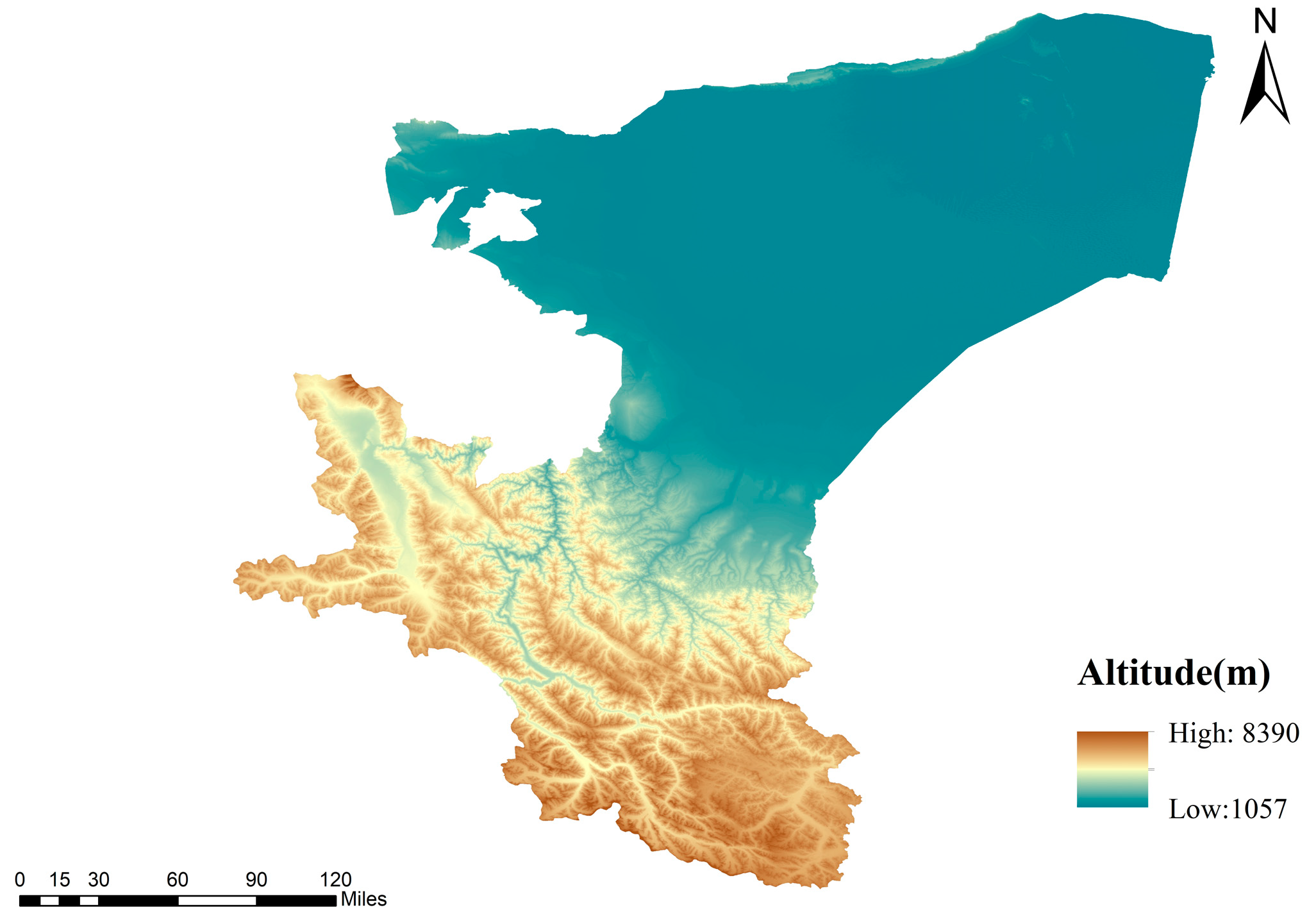
2.1. Study Area

Kashgar, formerly known as Shule, meaning “a place where jade gathers”, is situated in the westernmost region of Xinjiang Uygur Autonomous Region, China. Geographically, it is located between 71°39′ and 79°52′ east longitude, and 35°28′ and 40°16′ north latitude, encompassing a total land area of 1.62 × 10⁵ square kilometers [18]. With 12 cities and counties under its jurisdiction, Kashgar has a population of 4.51 million. Bordering or adjacent to eight countries, including Kyrgyzstan, Tajikistan, Afghanistan, Pakistan, and India, Kashgar serves as a confluence of Eastern and Western economies and cultures, and is the heart city of southern Xinjiang. It is a crucial gateway for China’s engagement with Central Asia and South Asia [19]. As a significant node on the ancient Silk Road, Kashgar was once the capital of Shule, one of the 36 countries in the Western Regions, boasting a profound historical and cultural heritage. In 1986, Kashgar was designated by the State Council as a famous historical and cultural city in China. The distribution of the study area is illustrated in Figure 1.

Kashgar is situated within a temperate continental climate zone, characterized by four distinct seasons, high evaporation rates, and spatially and temporally uneven precipitation [18]. The terrain exhibits a southwest-high, northeast-low topography, with dominant landforms comprising the Tarim Basin, Tianshan Mountains, and Kunlun Mountains trough fold belt [15]. Oases are concentrated in the region, with the Lyushgar and Yarkand River oases being particularly prominent. Water resources display a typical pattern of “spring drought, summer flood, autumn shortage, and winter dryness”, closely linked to the sensitivity of glacial meltwater and precipitation to temperature fluctuations [20]. The Pamir Plateau, Kunlun Mountains, and Kunlun Glaciers are extensively distributed, providing relatively stable water resources and serving as “solid water reservoirs”. However, the regional hydrological cycle system is fragile, with uneven temporal and spatial distribution of water resources [21]. By the mid-20th century, numerous large and small reservoirs had been constructed, boasting a total storage capacity of 1.339 billion cubic meters. With the exception of the Sujikake Reservoir, most reservoirs lack effective dead storage capacity.

Kashgar’s water system is significantly influenced by topography and regional precipitation. Rivers originate from glaciers and alpine snow belts, disappearing after traversing the plains. Influenced by mountain snowmelt, rivers exhibit pronounced annual low-water and flood variations. They are all fed by ice and snow meltwater, with the main streams themselves not generating flow. The region encompasses five major rivers and three short-distance rivers. The unique geographical environment has fostered two concentrated oases: the Yarkand River and Kashgar River basins [22]. The Yarkand River Basin features numerous tributaries, with the Keleqing and Taxkorgan rivers being the two primary tributaries. Originating from the northern Karakoram Mountains, they flow westward to southward, ultimately reaching the northeast. These are typical arid inland rivers, exhibiting “corridor oasis” characteristics. The Kashgar River Basin comprises six rivers: Kezi, Gaizi, Kushan, Aigziya, Chakmak, and Buguz rivers. Among these, the Kezi, Gaizi and Kushan rivers are the main tributaries, accounting for 91% of the average annual runoff of the Kashgar River Basin [23].

2.2. Data

2.2.1. Landsat Satellite Imagery

This study utilizes Landsat 5/7/8 satellite imagery as the primary data source, spanning the period from 2003 to 2023. The imagery possesses a temporal resolution of 16 days and a spatial resolution of 30 m. Surface reflectance products for Landsat 5 and Landsat 7 data were generated by the National Aeronautics and Space Administration (NASA) and the United States Geological Survey (USGS) using the Landsat Ecosystem Disturbance Adaptive Processing System (LEDAPS) algorithm. Landsat 8 surface reflectance products were generated using the Landsat Surface Reflectance Code (LASRC) algorithm [24]. All data have undergone radiometric correction and FLAASH atmospheric correction using USGS algorithms and are publicly accessible through the Google Earth Engine (GEE) platform.

2.2.2. Sentinel-2 Satellite Imagery

The Sentinel-2 satellite constellation comprises two satellites, Sentinel-2A and Sentinel-2B, launched in 2015 and 2017, respectively. Both satellites exhibit a revisit period of 10 days, achieving a 5-day revisit period when operating in tandem. Equipped with a multispectral sensor covering the visible to shortwave infrared spectrum, Sentinel-2 provides varying spatial resolutions across bands. This study utilizes Sentinel-2 data with a 10 m spatial resolution for water body extraction. Leveraging its high temporal and spatial resolution, Sentinel-2 enables effective monitoring of subtle changes in water bodies, thereby enhancing water body extraction accuracy.

2.2.3. Other Data

This study utilized precipitation and temperature data from the Climate Hazards Group Infrared Precipitation with Stations (CHIRPS) dataset (https://doi.org/10.1038/sdata.2015.66, accessed on 11 March 2025) and the NASA Land Processes Distributed Active Archive Center (LP DAAC) (https://doi.org/10.5067/MODIS/MOD11A2.061, accessed on 13 March 2025). Evapotranspiration data were obtained from the Moderate Resolution Imaging Spectroradiometer (MODIS) MOD16A2 dataset (https://doi.org/10.5067/MODIS/MOD16A2.006, accessed on 15 March 2025).

2.3. Methods

2.3.1. Water Body Extraction

This study evaluates five classification methods—Mahalanobis distance [25], minimum distance [26], maximum likelihood [27], support vector machine [28], and random forest [29]—to classify land cover using Sentinel-2 and Landsat imagery. This comparative analysis aims to identify the optimal classification algorithm and remote sensing data combination for the Kashgar region. Land cover is categorized into five classes: water bodies, deserts, vegetation, ice and snow, and built-up areas. This study focuses on assessing the accuracy of water body extraction.

This study focused on remote sensing imagery acquired from June to September, coinciding with the rainy season in Kashgar, a period conducive to the selection of suitable water body extraction methodologies. However, this period is characterized by vigorous vegetation growth, resulting in prevalent forest shadows and occasional cloud shadows within the imagery. These features exhibit spectral signatures similar to water bodies, posing a challenge for accurate classification. To enhance the discrimination between shadows and water bodies, this study incorporated auxiliary feature values, namely the Normalized Difference Water Index (NDWI) [30] and the Enhanced Vegetation Index (EVI) [31], into the extraction process, thereby mitigating classification errors. The NDWI and EVI are calculated as follows:

$$NDWI={\displaystyle \frac{{\rho }_{Green}-{\rho }_{NIR}}{{\rho }_{Green}+{\rho }_{NIR}}}$$

(1)

$$EWI={\displaystyle \frac{{\rho }_{Green}-({\rho }_{NIR}+{\rho }_{SWIR})}{{\rho }_{Green}+({\rho }_{NIR}+{\rho }_{SWIR})}}$$

(2)

where ${\rho }_{Green}$, ${\rho }_{NIR}$, and ${\rho }_{SWIR}$ represent the reflectance values in the green, near-infrared, and short-wave infrared bands, respectively. For Landsat 5 imagery, ${\rho }_{Green}$, ${\rho }_{NIR}$, and ${\rho }_{SWIR}$ correspond to bands 2, 4, and 5, respectively; for Landsat 8 imagery, they correspond to bands 3, 5, and 6, respectively.

2.3.2. Data Analysis Methods

This study employed the Theil–Sen slope estimator [32] and the Mann–Kendall (MK) test [33] to analyze temporal trends in water area changes within the Kashgar region. These non-parametric methods are widely utilized for trend analysis due to their robustness and flexibility. The Theil–Sen estimator provides a robust measure of trend magnitude, exhibiting resilience to outliers and measurement errors, making it particularly suitable for long-term time series data. The MK test, on the other hand, assesses the significance of monotonic trends in time series data without requiring assumptions of normality or linearity [34]. Furthermore, the MK test possesses the capability to identify abrupt shifts or change points within the data [35].

This study employed visual interpretation and kernel density analysis to investigate the spatiotemporal dynamics of water bodies in the Kashgar region from 2003 to 2023. The visual interpretation provided a qualitative assessment of water body changes, while the kernel density analysis offered a quantitative evaluation of their spatial distribution patterns, particularly for dispersed water bodies such as lakes. Kernel density estimation, a non-parametric technique, constructs a smoothed probability density function by convolving a kernel function with each data point, assigning weights based on distance [36]. This approach enables the quantification of spatial clustering or dispersion of point features.

This study investigated the seasonal trends and changes in water area extent in the Kashgar region from 2003 to 2023, utilizing water inundation frequency (WIF) data. WIF, defined as the ratio of inundation occurrences at a given location to the total number of inundation events within a specified period, serves as an indicator of regional inundation patterns. WIF is calculated by dividing the number of times a pixel is inundated by the total number of inundation events across the time series [37]. Mathematically, WIF can be expressed as:

$$WIF={\displaystyle \frac{{\sum }_{j=1}^N{W}_{i,j}}{{\sum }_{j=1}^N{O}_{i,j}}}\times 100\%$$

(3)

where $N$ denotes the total number of valid observed pixels; $W_{i,j}$ is a binary variable representing the inundation status of the ith pixel in the jth image (1 indicating inundation, 0 indicating no inundation); and $O_{i,j}$ denotes the observation status of the ith pixel in the jth image (1 indicating observed, 0 indicating unobserved).

To mitigate noise artifacts arising from cloud cover, shadowing, and resolution constraints, the 25th and 75th percentiles of water inundation frequency (WIF) are adopted as primary segmentation thresholds, consistent with established methodologies [6,38]. Pixels with WIF values below the 25th percentile were classified as non-water bodies. Pixels exceeding the 25th percentile were further categorized into two classes: permanent water bodies (characterized by year-round presence and insensitivity to seasonal variations, with WIF values ranging from 0.75 to 1) and seasonally fluctuating water bodies (exhibiting inundation extent variations across seasons, with WIF values ranging from 0.25 to 0.75).

2.4. Accuracy Assessment

This study employed six metrics to evaluate classification accuracy: overall accuracy (OA), Kappa coefficient (Kappa), misclassification error (CE), omission error (OE), producer accuracy (PA), and user accuracy (UA). OA provides a general measure of classification effectiveness [39], while the Kappa coefficient assesses both the accuracy and reliability of the classifier, with values closer to 1 indicating superior performance [40]. CE [41] and OE [42] quantify the discrepancies between the classified image and the reference image, specifically measuring the overall misclassification rate and the degree to which a particular ground cover type is misclassified, respectively. PA [43] and UA [44] evaluate the probability of correctly classifying a specific land cover type, with PA emphasizing the accuracy of the classification map and UA focusing on the reliability of the classification results. Notably, CE, OE, PA, and UA were evaluated exclusively for water bodies.

This study employed a multi-step approach to investigate spatiotemporal changes in water bodies within the Kashgar region. First, Landsat imagery (2003–2023) and Sentinel-2 imagery (2013–2023) were acquired from the Google Earth Engine (GEE) platform. Images with cloud cover of less than 15% were selected and masked. Second, five water body extraction methods (Mahalanobis distance, minimum distance, maximum likelihood, support vector machine, and random forest) were evaluated using Landsat 8 and Sentinel-2 imagery from June to September 2023. Accuracy assessment revealed that the random forest algorithm yielded the highest accuracy and was subsequently employed for water body extraction. Third, water body areas were quantified from 2003 to 2023. Temporal trends were analyzed using correlation analysis, Sen’s slope estimation, and the Mann–Kendall test. Spatial patterns were examined through visual interpretation and kernel density analysis. Fourth, the overall area, permanent area, and seasonal area of water bodies were quantified to further elucidate spatiotemporal dynamics. Finally, the influence of precipitation, temperature, evaporation, and regional climate on water body changes was assessed.

3. Results and Analysis

3.1. Accuracy Evaluation Analysis

To validate the accuracy of the five aforementioned extraction methods, this study utilized Landsat and Sentinel-2 imagery acquired from June to September 2023, covering the Kashgar region. The results are presented in

Table 1. Comparison of classification accuracy for five methods applied to two satellite image types in 2023.

Methods	Image	OA	Kappa	CE	OE	PA	UA
Mahalanobis Distance	Sentinel-2	78.95%	0.7303	1.61%	39.58%	60.42%	98.39%
	Landsat 8	82.76%	0.7816	1.18%	24.46%	75.54%	98.82%
Minimum Distance	Sentinel-2	61.54%	0.5010	1.63%	30.89%	69.11%	98.37%
	Landsat 8	75.00%	0.6889	8.72%	4.31%	95.69%	91.28%
Maximum Likelihood	Sentinel-2	70.37%	0.6333	0.73%	8.45%	91.55%	99.27%
	Landsat 8	82.86%	0.7780	0.65%	2.85%	97.15%	99.35%
Support Vector Machine	Sentinel-2	81.82%	0.7596	0.69%	0.71%	99.29%	99.31%
	Landsat 8	85.71%	0.8149	0.36%	0.44%	99.56%	99.64%
Random Forest	Sentinel-2	97.10%	0.9005	0.21%	0.41%	99.59%	99.79%
	Landsat 8	95.00%	0.9889	0.26%	0.48%	99.52%	99.74%

. The Random Forest algorithm demonstrated robust performance across both Landsat and Sentinel-2 imagery, achieving an average overall accuracy of 96.05% and an average water body accuracy of 99.87%, with minimal misclassification or omission errors. Notably, Sentinel-2 imagery exhibited the highest overall accuracy, reaching 97.10%, with a corresponding water body accuracy of 99.79%. Conversely, the lowest overall accuracy (95.00%) and water body accuracy (99.74%) were observed for Landsat 8 imagery. In summary, the Random Forest algorithm exhibits strong robustness, high accuracy, and broad applicability, making it an ideal choice for water area extraction in the Kashgar region.

To ensure the consistency and accuracy of water body extraction, this study utilized Landsat imagery from 2003 to 2018 and Sentinel-2 imagery from 2019 to 2023 for water body delineation in the Kashgar region, referencing previous research findings. This approach was adopted based on the observation that Sentinel-2 imagery demonstrated superior overall accuracy in water body extraction for the Kashgar region from 2019 to 2023 compared to Landsat 8 imagery.

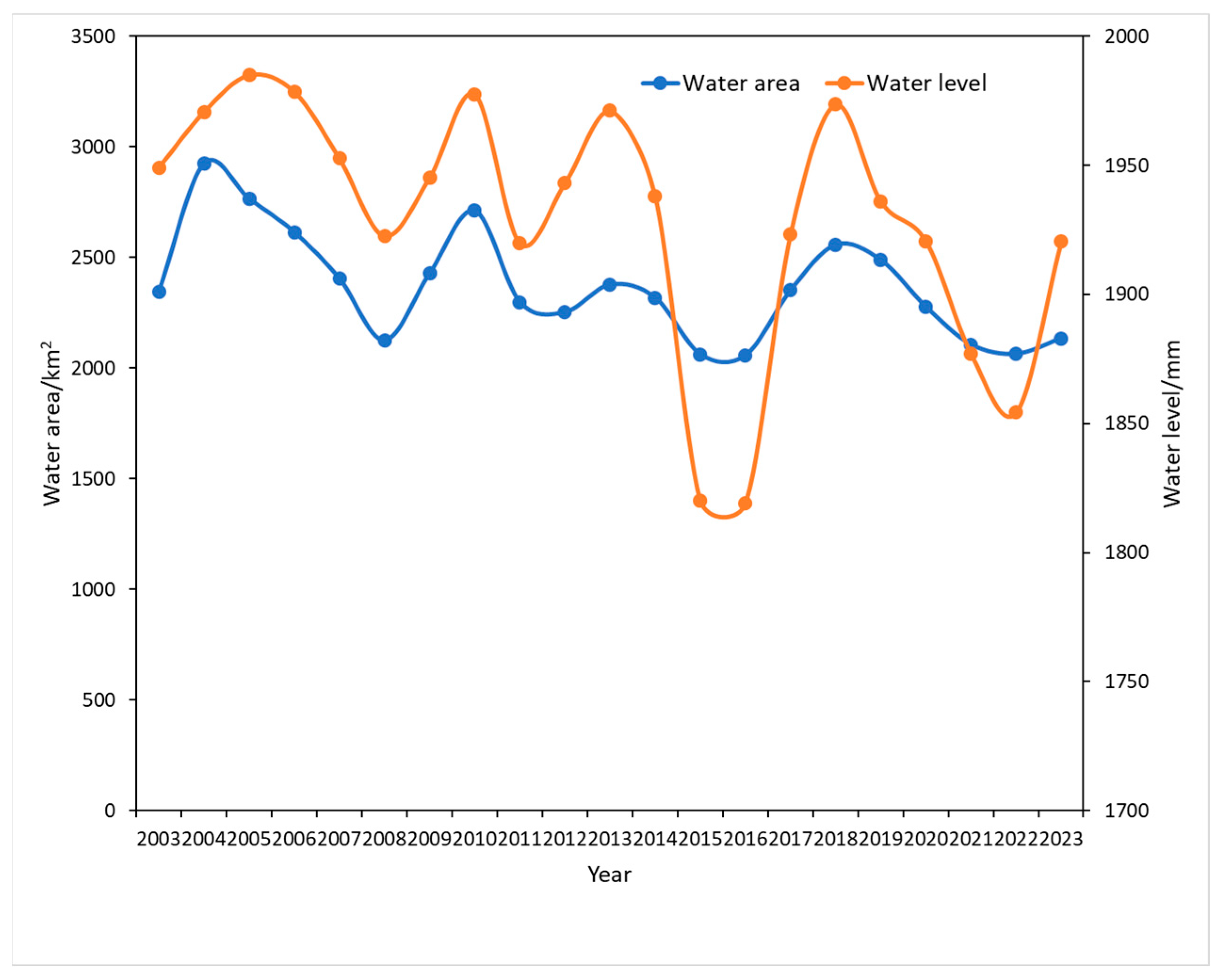
3.2. Temporal Characteristics of Annual Water Area Changes in the Kashgar Region

Figure 2 shows the statistical results of the changes in the water area in Kashgar from 2003 to 2023; the water area in the Kashgar region exhibited a fluctuating downward trend, with an average annual change rate of −11.17 km²/year. A detailed analysis is as follows: in 2003–2004, water area increased to a maximum of 2924.765 km², representing an increase of 576.63 km² and a growth rate of 24.72%; in 2004–2016, water area generally decreased, but displayed fluctuating changes, reaching a minimum of 2057.83 km² in 2016. The most significant decrease occurred in 2007, with a reduction of 280.42 km² and a growth rate of −11.55%; in 2016–2018, water area increased, with the most substantial increase occurring in 2016, reaching 294.32 km² and a growth rate of 14.32%; and in 2018–2023, water area exhibited an overall decrease, characterized by fluctuating changes. The largest decrease occurred in 2019, with a reduction of 211.61 km² and a growth rate of −8.5%.

To characterize the temporal trends in water area changes within the Kashgar region, this study employed Sen’s slope estimator, the Mann–Kendall (MK) test, and change point analysis.

The analysis of the time series of water area change in the Kashgar region from 2003 to 2023 revealed a Sen’s slope estimate of −0.52, indicating an overall downward trend. The significance of this trend was assessed using the Mann–Kendall (MK) test. As shown in Figure 3, the estimated Sen’s slope for water area changes in the Kashgar region passed the 0.95 confidence level, confirming the statistical significance of the decreasing trend. The change point analysis identified a shift in water area in 2011, with a significant decrease observed in that year. A consistent upward trend was evident from 2003 to 2010, followed by a sustained downward trend from 2012 to 2023.

Utilizing the water inundation frequency method and interannual water area statistics for the Kashgar region, this study characterized the interannual distribution of permanent and seasonal water bodies. From 2003 to 2023, the overall trend of seasonal water area changes mirrored the trend of total water area changes, exhibiting a fluctuating downward trend with an average annual change rate of −12.80 km²/year. As depicted in Figure 4a, the seasonal water body area increased by 290.142 km² between 2003 and 2004, representing a growth rate of 21.70%, reaching a maximum of 1627.339 km² in 2004. Subsequently, the seasonal water body area fluctuated and decreased, reaching a minimum of 1081.229 km² in 2023. The largest area change occurred in 2010, with a decrease of 407.163 km² and a growth rate of −26.08%. In contrast, the permanent water body area in the Kashgar region generally exhibited a fluctuating upward trend, with an average annual change rate of 2.28 km²/year. From 2003 to 2004, the permanent water body area increased by 289.486 km², representing a growth rate of 28.72%, reaching a maximum of 1297.426 km² in 2004. From 2004 to 2022, the permanent water body area fluctuated and decreased, reaching a minimum of 855.972 km² in 2022. The largest area change occurred in 2008, with an increase of 185.890 km² and a growth rate of 18.17%. Between 2022 and 2023, the permanent water body area increased by 225.257 km², representing a growth rate of 26.32%. The comparison of changes in permanent and seasonal water areas with total water area and the proportion of seasonal water bodies (Figure 4a,b) reveals that seasonal water area in Kashgar constitutes 50–60% of the total water area, reaching a minimum of 49.86% in 2007. Considering the characteristics of water area fluctuations, overall water area changes in Kashgar are driven by variations in both permanent and seasonal water areas, with the contribution of seasonal water area changes slightly exceeding that of permanent water area changes.

To characterize the trends in the permanent and seasonal water body area changes within the Kashgar region, this study employed Sen’s slope estimation, the Mann–Kendall (MK) test, and change point analysis. The Sen’s slope estimate for the permanent water body area changes from 2003 to 2023 was 0.42, indicating a slight overall upward trend. Conversely, the Sen’s slope estimate for the seasonal water body area changes was −0.16, suggesting a slight downward trend. To assess the significance of these trends, the MK test was applied (Figure 4c,d). The Sen’s slope estimates for the permanent water body area changes passed the 0.95 confidence level, confirming the statistical significance of the increasing trend. No distinct change points were identified for the permanent water body area, failing the 0.95 confidence test only in 2013. From 2003 to 2013, the permanent water body area exhibited a significant downward trend, while from 2013 to 2023, a significant upward trend was observed. The Sen’s slope estimate for the seasonal water body area changes did not pass the 0.95 confidence test, indicating a non-significant decreasing trend. A change point was identified in 2006, with a significant decrease in the seasonal water body area. From 2003 to 2006, the seasonal water body area displayed a stable upward trend, followed by a stable downward trend from 2006 to 2023.

To validate the experimental findings, the upper reaches of the Yarkand River, a representative water body in the Kashgar region, were selected as the validation site. Situated in the high-altitude mountainous terrain west of Kashgar, this area receives the majority of the river’s recharge, making it an ideal location for result verification. The water level data for the upper Yarkand River from 2003 to 2023 were obtained from the Kuruklangan (III) hydrological station, located in Datong Township, Taxkorgan County. As illustrated in Figure 5, the water level data from this station exhibits a strong correlation with the temporal trends in water body area change observed across Kashgar. This concordance lends credence to the accuracy and reliability of the experimental results, providing robust data support for local policymakers. By elucidating the dynamics of water body change in Kashgar, these findings can inform the development of evidence-based policies that promote sustainable development and safeguard the region’s ecological integrity.

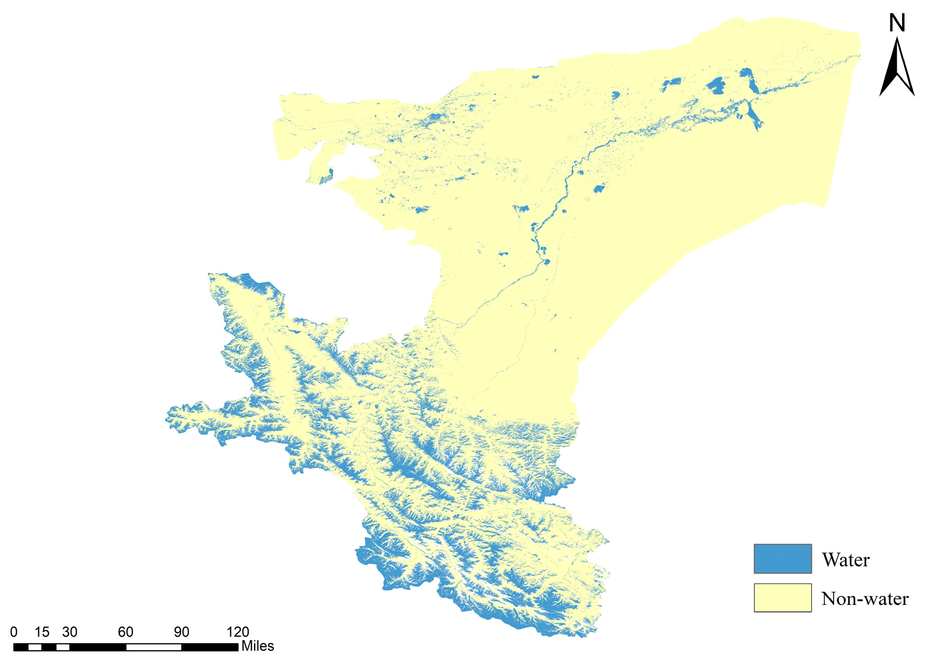
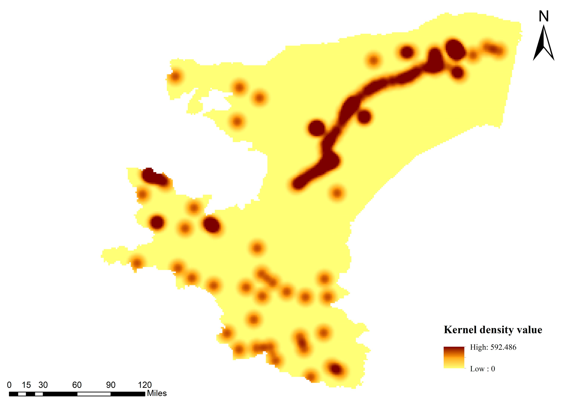
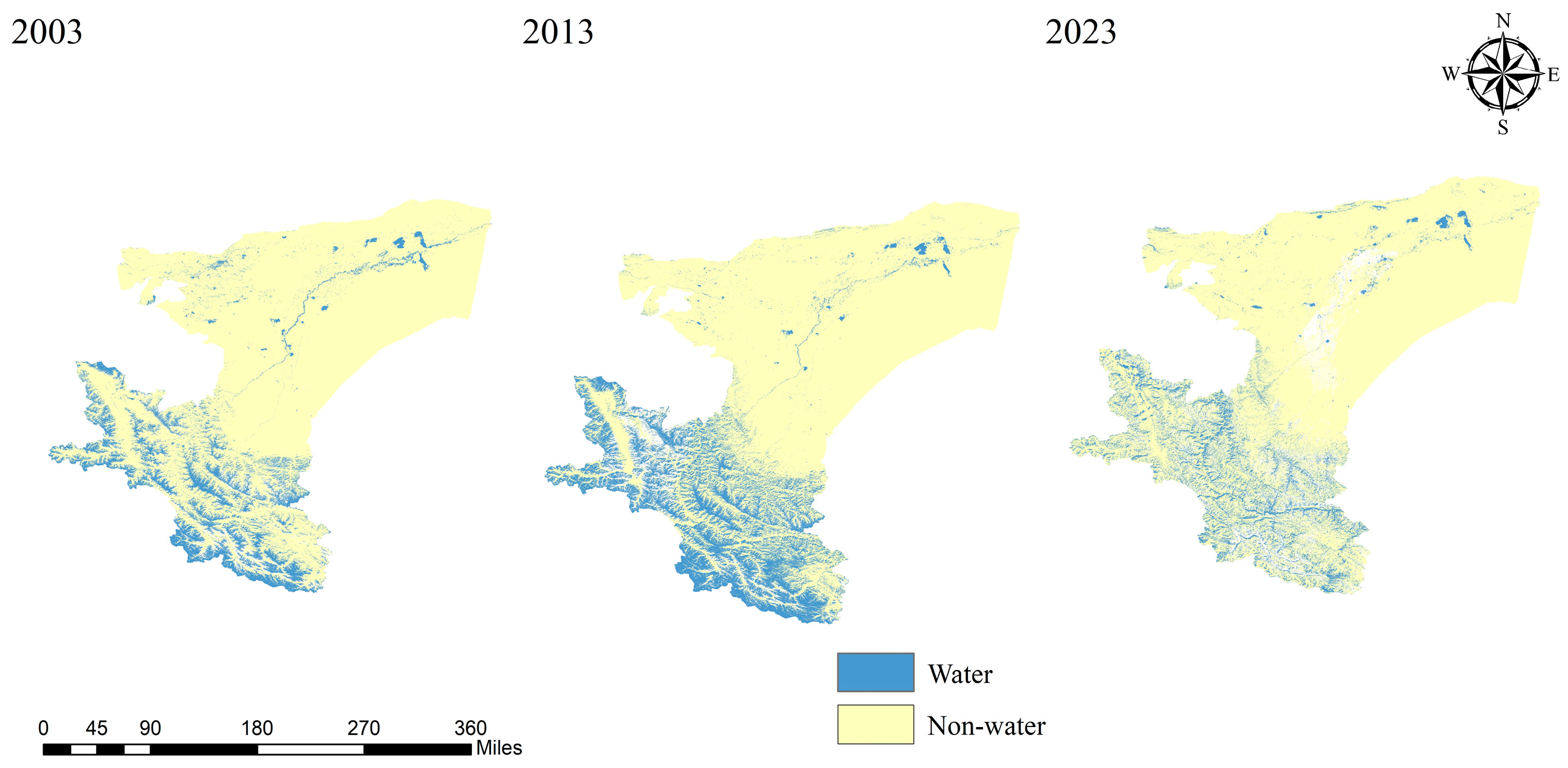
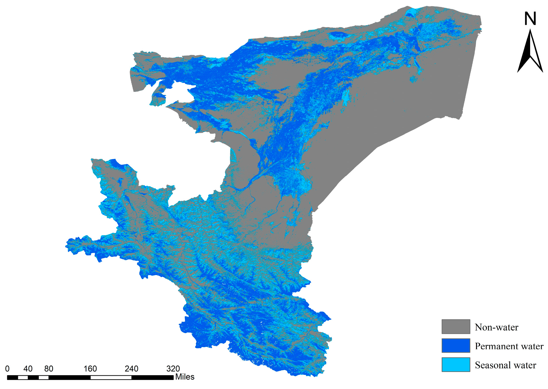
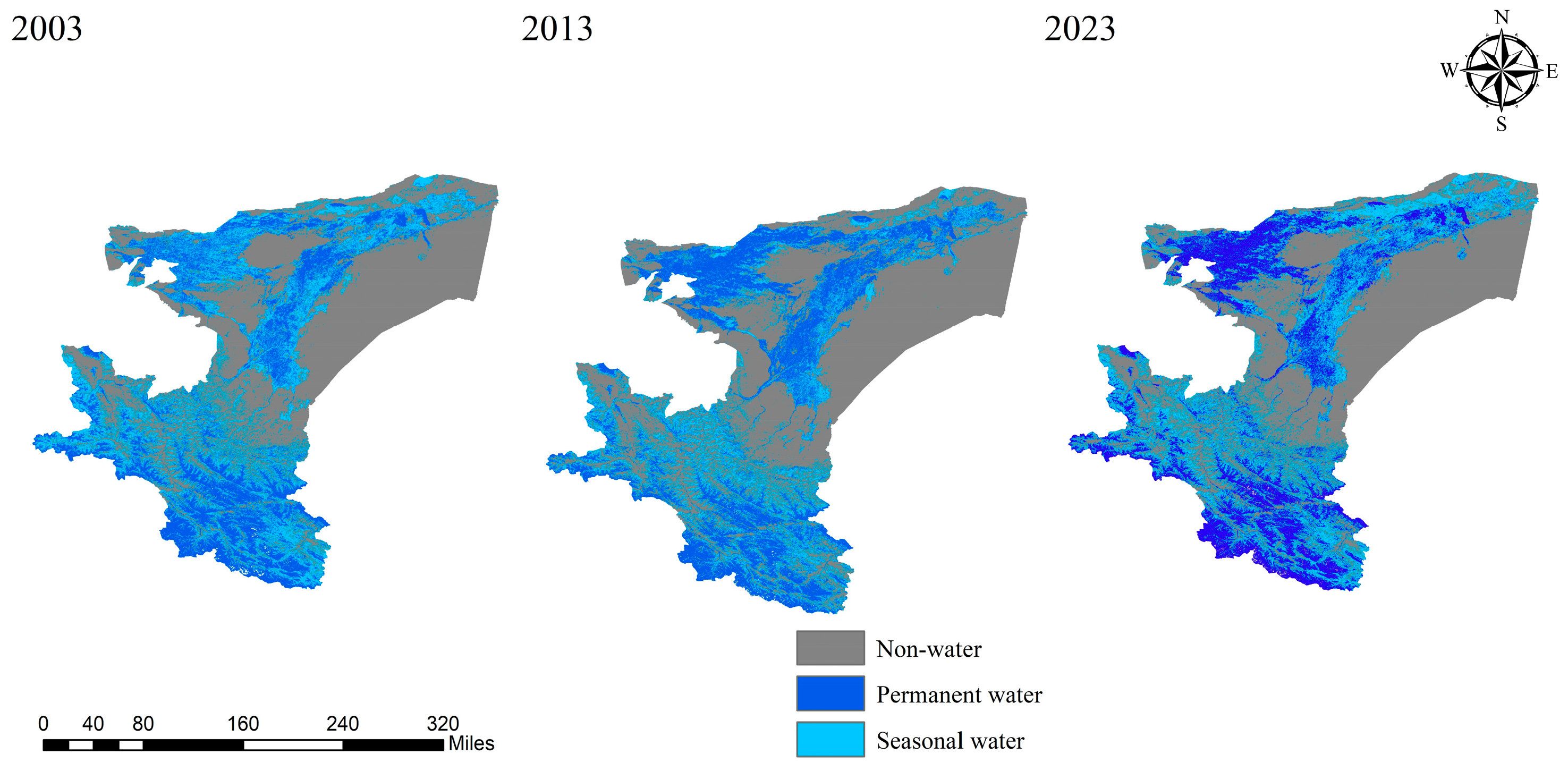
3.3. Spatial Patterns of Water Area Changes in the Kashgar Region

Figure 6 reveals distinct regional variations in the spatial distribution of water bodies across Kashgar. A high density of large lakes is observed in the southwest, whereas a mixture of large and small lakes characterizes the northeast and desert interior. These two regions are interconnected by a major river system. Given the abundance of lakes within the study area, kernel density analysis was employed to characterize the spatial distribution patterns of water bodies in Kashgar. The findings are presented below.

Figure 7 illustrates distinct regional variations in the spatial distribution of water bodies across the Kashgar region. While rivers traverse the northeast and southwest, lakes exhibit clear clustering patterns in the west, south, and northeast. Weaker clustering is observed in the central and western desert hinterlands and the northwest, whereas other regions lack discernible lake clustering.

The spatial dynamics of water bodies in Kashgar exhibit considerable complexity, with distinct trends in area change observed across different water body types. Recognizing that long-term time series are essential to capture the nuances of water body spatial change, this study employed a decadal cycle to extract water body information for Kashgar in 2003, 2013, and 2023 for comparative analysis. The findings are presented in the accompanying figure.

Figure 8 illustrates pronounced interannual variability in the spatial distribution of water bodies within the Kashgar region. Between 2003 and 2013, a notable increase in both the number and area of lakes was observed in the western and southern portions of the region, whereas lakes in the western and northern areas exhibited a slight decline in extent. From 2013 to 2023, a significant reduction in both the number and area of lakes in the west and south was evident, accompanied by a downward trend in riverine area. Conversely, the central and northern regions experienced an increase in both the number and area of lakes, potentially attributable to the formation of ephemeral lakes due to river desiccation. Overall, the total water body area in Kashgar exhibited an initial increase followed by a subsequent decrease between 2003 and 2023.

Figure 9 depicts the spatial distribution of the permanent and seasonal water bodies in the Kashgar region. Both types exhibit a dispersed pattern, occurring in the southwestern mountainous area, central, northern, and western portions of the study area. Seasonal water bodies are predominantly located in proximity to permanent water bodies, suggesting a well-connected hydrological cycle and widespread distribution of aquatic features such as rivers and lakes. The water bodies in the southern mountainous regions display seasonal fluctuations, potentially linked to glacial melt driven by rising temperatures.

This study conducted a decadal analysis of permanent and seasonal water bodies in the Kashgar region, extracting data for 2003, 2013, and 2023. The findings are presented in Figure 10.

Figure 10 illustrates pronounced interannual variability in the spatial distribution of permanent and seasonal water bodies within the Kashgar region. Between 2003 and 2013, a notable increase in the extent of permanent water bodies was observed in the northwestern and central portions, accompanied by a significant reduction in the seasonal water body area. Conversely, the permanent water bodies in the south exhibited a slight decline, while the seasonal water bodies showed a slight increase. From 2013 to 2023, the central permanent water body area decreased substantially, whereas the seasonal water body area increased significantly. The permanent water bodies in the northwest, south, and northeast displayed decreasing trends, while the seasonal water bodies exhibited increasing trends. Overall, the total water body area in Kashgar exhibited an initial increase followed by a subsequent decrease between 2003 and 2023. This pattern was also reflected in the trends of the permanent water bodies, which initially increased and then decreased, while the seasonal water bodies showed an overall decreasing trend.

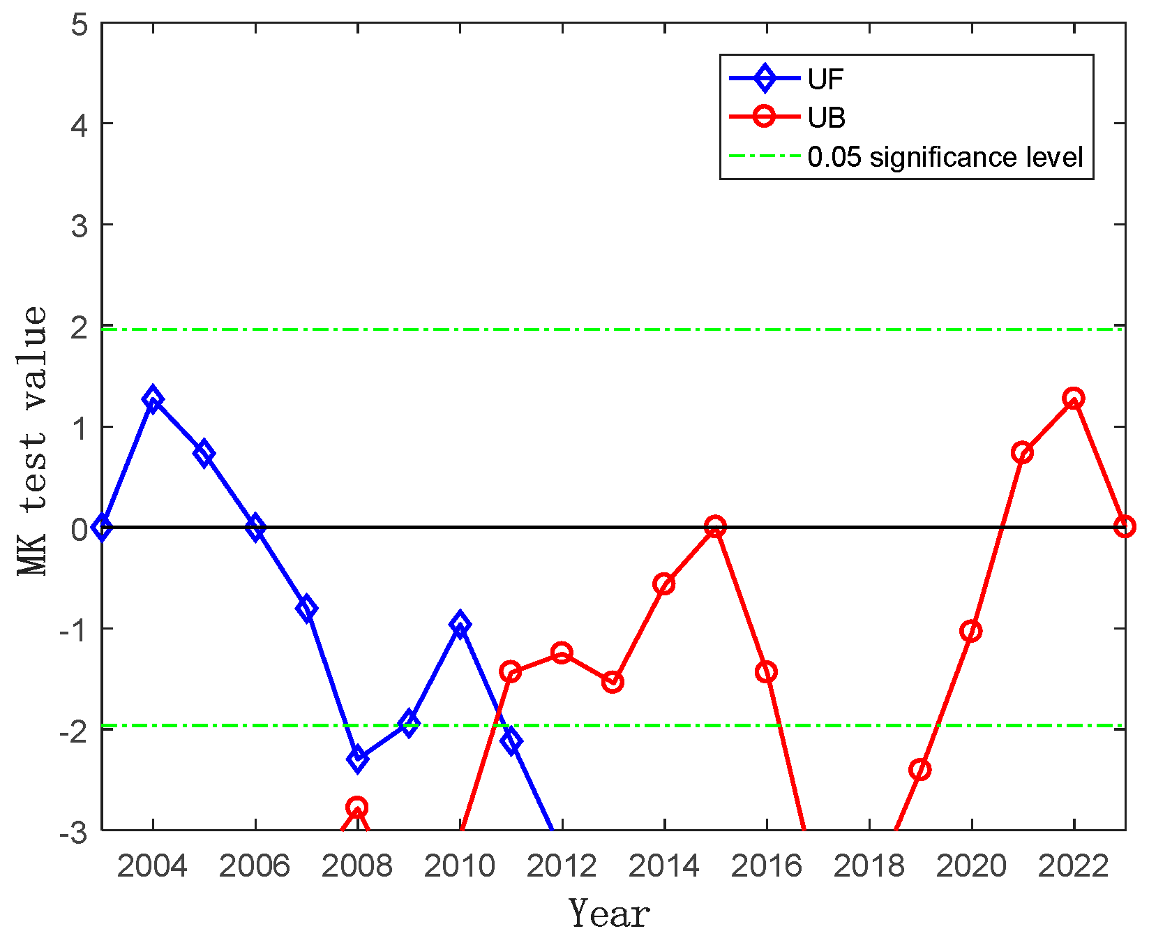
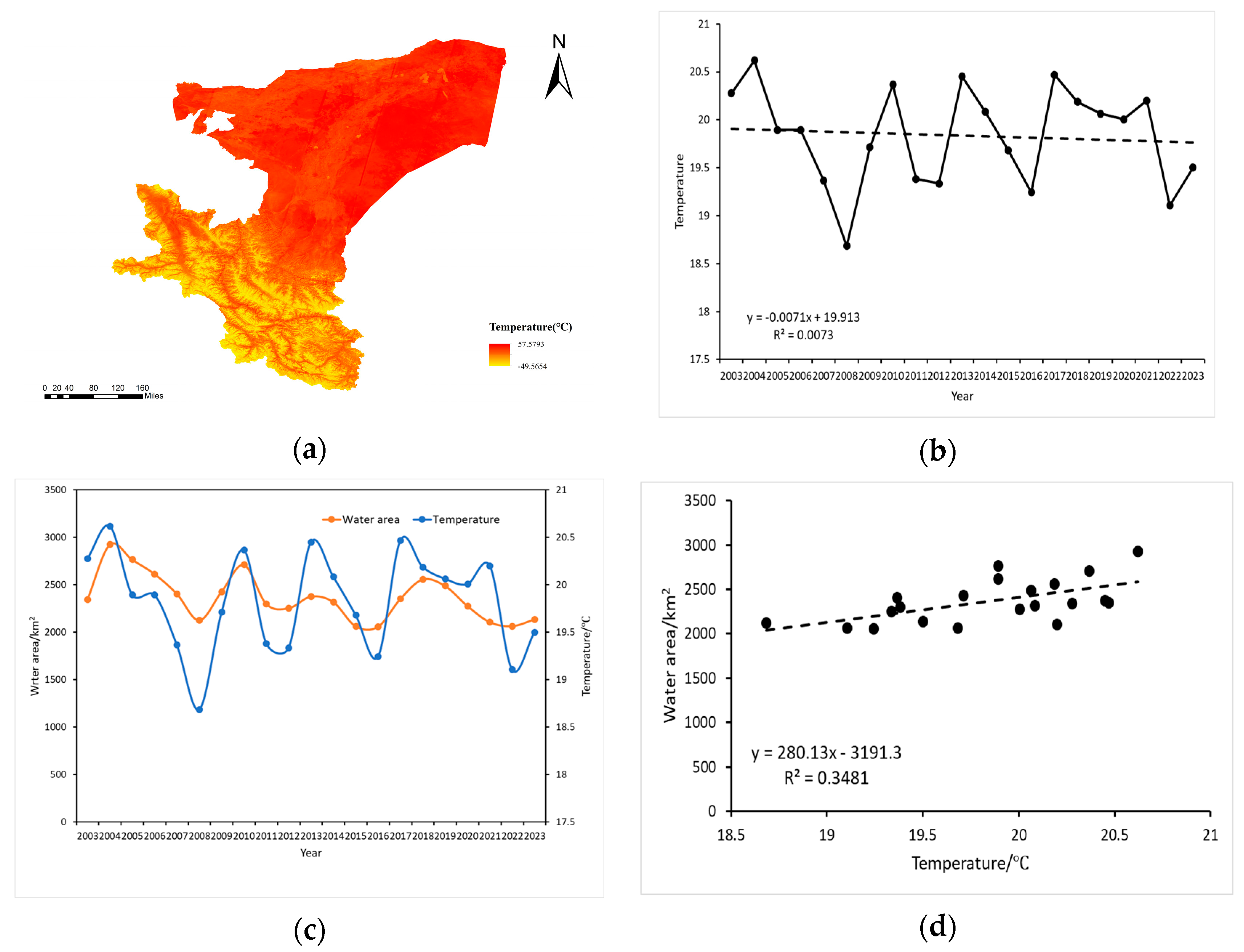
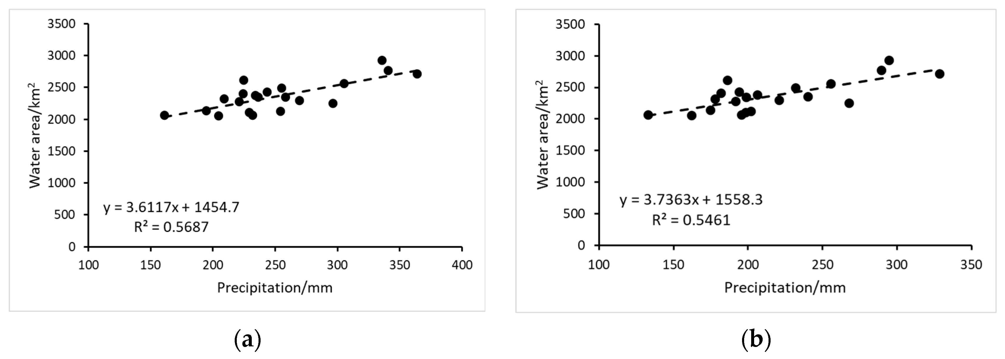
3.4. Drivers of Water Body Area Change in the Kashgar Region

Precipitation is a crucial driver of water body area change, particularly in regions with high precipitation levels, where it serves as the primary determinant of water body dynamics. In the Kashgar region, seasonal water bodies constitute 50–60% of the total water body area, highlighting the significant influence of precipitation on water body fluctuations. This study investigates the correlation between changes in water body area and precipitation to elucidate the mechanisms by which precipitation variability impacts water body dynamics. Specifically, we analyzed the relationship between water body area and annual average rainfall in Kashgar from 2003 to 2023. Figure 11a depicts the spatially heterogeneous distribution of precipitation in Kashgar, with concentrations primarily in the southern and western regions, while the central, eastern, and northern regions experience relatively lower precipitation. Figure 11b reveals a general downward trend in annual average precipitation from 2003 to 2023, exhibiting an average annual change rate of −3.86666 mm/year. Precipitation peaked in 2010 (233.818 mm) and reached its minimum in 2022 (107.188 mm). Figure 11c illustrates the temporal trends of surface water area and annual precipitation in Kashgar from 2003 to 2023, demonstrating a general concordance between the two trends. This suggests that precipitation is a key factor influencing inland water area changes in Kashgar. Furthermore, Figure 11d reveals a statistically significant positive correlation between changes in surface water area and average annual precipitation, although the correlation coefficient (R²) is relatively weak (0.2431). The extremely low p-value (2.6 × 10⁻³⁴ < 0.05) strongly supports the conclusion that precipitation is a direct and important driver of surface water area changes.

Given the increasing global warming trend and accelerated water cycle, this study further investigated the relationship between surface water area and annual average temperature in Kashgar. Figure 12a illustrates a decreasing temperature gradient from southwest to northeast, with the southwest exhibiting the lowest temperatures, likely influenced by topographic factors. Figure 12b reveals a general downward trend in annual average temperature from 2003 to 2023, with an average annual change rate of −0.03885 °C/year. The highest temperature was recorded in 2002 (20.62 °C), while the lowest temperature occurred in 2008 (18.686 °C). Figure 12c depicts the temporal trends of surface water area and annual average temperature, demonstrating a general concordance between the two trends. This suggests that temperature is a significant factor influencing inland water area changes in Kashgar. Furthermore, Figure 12d reveals a statistically significant positive correlation between changes in surface water area and annual average temperature. Although the correlation coefficient (R²) is relatively weak (0.3481), the extremely low p-value (1.8 × 10⁻³⁵ < 0.05) strongly supports the conclusion that temperature is a direct and important driver of surface water area changes.

Evapotranspiration is a pivotal process within the terrestrial water cycle, playing a crucial role in understanding the water cycle’s response to climate change and anthropogenic activities. Rising temperatures are projected to enhance evaporation rates, consequently diminishing surface runoff recharge. This study investigated the relationship between surface water area and mean annual evapotranspiration in the Kashgar region. As depicted in Figure 13a, evapotranspiration in the Kashgar region exhibited a fluctuating upward trend from 2003 to 2023, with an average annual change rate of 11.99885 mm. Evapotranspiration peaked in 2021 (2153.88 mm), diverging from the temperature peak, while the lowest value occurred in 2007 (1265.339 mm). Figure 13b illustrates the temporal trends of surface water area and mean annual evapotranspiration in the Kashgar region from 2003 to 2023. A discernible downward trend in surface water area contrasted with an upward trend in evapotranspiration, indicating largely inconsistent patterns. Further analysis revealed a negative correlation between surface water area and mean annual temperature (correlation coefficient = 0.0631), as shown in Figure 13c. This suggests that evapotranspiration may act as an indirect driver of surface water area changes.

The source of surface water recharge in Kashgar remains a subject of ongoing debate within the scientific community, with no definitive consensus reached. This study aims to elucidate the relationship between surface water recharge in Kashgar and regional climate change by investigating the correlation between changes in Kashgar’s water area and climatic factors in its surrounding regions. This analysis seeks to provide a scientific foundation for a deeper understanding of the region’s hydrological cycle characteristics. Given Kashgar’s topography, which is characterized by higher elevations in the southwest and lower elevations in the northeast, with most rivers and lakes originating from the southwestern mountainous areas and distributed along the slopes, this study selected annual average precipitation data from Taxkorgan County and Yecheng County, located in Kashgar’s southwestern mountainous region. The objective is to analyze the potential relationship between the trends in these climatic variables and changes in Kashgar’s water area.

Figure 14a reveals a statistically significant positive correlation between changes in Kashgar’s surface water area and the average annual precipitation in Taxkorgan County (R² = 0.5687, p = 2.4 × 10⁻³³ < 0.05). This strong correlation indicates that precipitation in Taxkorgan County is a significant driver of surface water area fluctuations in Kashgar. Similarly, Figure 14b demonstrates a significant positive correlation between changes in Kashgar’s surface water area and average annual precipitation in Yecheng County (R² = 0.5461, p = 1.2 × 10⁻³³ < 0.05). This finding further supports the conclusion that precipitation in Yecheng County plays a crucial role in influencing surface water dynamics in Kashgar. This study also investigated the relationship between changes in Kashgar’s water area and average annual temperature and evaporation in Taxkorgan and Yecheng Counties. However, these analyses did not reveal statistically significant correlations (p > 0.05), suggesting that temperature and evaporation in these surrounding areas are not primary drivers of surface water area fluctuations in Kashgar. In contrast, precipitation in the surrounding areas emerged as the key factor influencing changes in Kashgar’s water area.

4. Discussion

4.1. Water Extraction Methodologies in the Kashgar Region

This study evaluated the performance of five water body extraction methods: Mahalanobis distance, minimum distance, maximum likelihood, support vector machine (SVM), and random forest (RF) algorithms within the Kashgar region. The results indicated that the Mahalanobis distance, minimum distance, and maximum likelihood methods yielded suboptimal overall accuracy, user accuracy, and Kappa coefficients, primarily due to misclassification of water bodies. These methods exhibited limitations in distinguishing water bodies from spectrally similar features such as shadows and glaciers. While SVM demonstrated relatively higher accuracy, its requirement for feature normalization during data preprocessing rendered it computationally intensive for the study’s extensive temporal and spatial scales. In contrast, the RF algorithm achieved a favorable balance between accuracy and processing efficiency, proving to be the most suitable method for large-scale water body extraction in the Kashgar region.

4.2. Socioeconomic Influences on Water Area Dynamics in Kashgar

Over the past few decades, particularly since 2014 [45], the Kashgar region has undergone rapid population growth and economic development. This has fueled industrialization and urbanization, leading to the conversion of surface water bodies into farmland or construction land. Consequently, the area of water bodies in Kashgar has exhibited a continuous decline between 2003 and 2023.

Literature findings [45] indicate that since 1972, cultivated land in Kashgar has expanded continuously, urbanization has intensified, and the area of forests and water bodies has shown a downward trend. Snow cover has also been subject to fluctuations driven by both climate change and anthropogenic activities. These changes, in turn, influence snow and ice melt and runoff patterns, ultimately impacting water body dynamics across the entire Kashgar region.

According to [46], the ecological security of the Kashgar region is transitioning from a state of “overall security” to “relative security” and ultimately towards “security”. This trajectory suggests a positive outlook for the protection and enhancement of local water security. The future ecological prospects for the Kashgar region appear relatively optimistic.

4.3. Uncertainties of This Study

Due to the extensive temporal and spatial scale of this study, the utilization of high spatial resolution satellite imagery, while desirable, was constrained by the limitations of revisit frequency, hindering the continuous monitoring of dynamic water body changes. The 30 m spatial resolution employed in this study resulted in the omission of narrow water bodies, such as ponds and ditches. Future research should integrate optical imagery with ground-based observations to enhance the accuracy of water body delineation.

Given the arid nature of the Kashgar region, characterized by complex oasis and desert landscapes, MODIS-derived evapotranspiration estimates may exhibit inherent biases. The sparse vegetation cover in arid environments complicates the differentiation between soil evaporation and vegetation transpiration. Subsequent studies should leverage unmanned aerial vehicles (UAVs) or Sentinel-2 data for more precise evapotranspiration estimations.

This study encountered challenges in effectively distinguishing ice and snow from water bodies. Future research should refine model accuracy and comprehensively analyze the influence of ice and snow melt on local water area variations. During the water level data collection process, inconsistencies were identified in the water level records of several reservoirs. Future studies should implement in situ monitoring devices for long-term water level observations.

5. Conclusions

This study investigated the spatiotemporal dynamics of water bodies in Kashgar, Xinjiang, China, from 2003 to 2023, utilizing Landsat and Sentinel-2 imagery. Water bodies were delineated using a random forest algorithm. The results revealed a fluctuating trend in the total water area, exhibiting a slight overall decrease. The seasonal variations mirrored this trend, displaying a fluctuating downward trajectory. Conversely, the permanent water bodies demonstrated an upward trend. The statistical analysis indicated a positive correlation between water area and both precipitation and temperature, and a negative correlation with evaporation. Notably, precipitation in Taxkorgan and Yecheng counties, influenced by topographic factors, exerted a significant impact on water area changes, exhibiting strong correlations (R² = 0.5687 and 0.5461, respectively). This highlights the crucial role of regional climatic factors in shaping the overall dynamics of water bodies in Kashgar. These findings provide a robust scientific foundation for developing effective regional water resource management policies and ecological conservation strategies.

References

1. Zhang, Y.; Li, C.; Chiew, F.H.S.; Post, D.A.; Zhang, X.; Ma, N.; Tian, J.; Kong, D.; Leung, L.R.; Yu, Q.; et al. Southern Hemisphere dominates recent decline in global water availability. Science 2023, 382, 579–584. [Google Scholar] [CrossRef] [PubMed]
2. Carroll, M.L.; Townshend, J.R.; DiMiceli, C.M.; Noojipady, P.; Sohlberg, R.A. A new global raster water mask at 250 m resolution. Int. J. Digit. Earth 2009, 2, 291–308. [Google Scholar] [CrossRef]
3. Cole, J.J.; Prairie, Y.T.; Caraco, N.F.; McDowell, W.H.; Tranvik, L.J.; Striegl, R.G.; Duarte, C.M.; Kortelainen, P.; Downing, J.A.; Middelburg, J.J.; et al. Plumbing the global carbon cycle: Integrating inland waters into the terrestrial carbon budget. Ecosystems 2007, 10, 172–185. [Google Scholar] [CrossRef]
4. Wada, Y.; van Beek, L.P.H.; Viviroli, D.; Dürr, H.H.; Weingartner, R.; Bierkens, M.F.P. Global monthly water stress 2: Water demand and severity of water stress. Water Resour. Res. 2011, 47, W07518. [Google Scholar] [CrossRef]
5. Pekel, J.-F.; Cottam, A.; Gorelick, N.; Belward, A.S. High-resolution mapping of global surface water and its long-term changes. Nature 2016, 540, 418–422. [Google Scholar] [CrossRef]
6. Zou, Z.; Xiao, X.; Dong, J.; Qin, Y.; Doughty, R.B.; Menarguez, M.A.; Zhang, G.; Wang, J. Divergent trends of open-surface water body area in the contiguous United States from 1984 to 2016. Proc. Natl. Acad. Sci. USA 2018, 115, 3810–3815. [Google Scholar] [CrossRef]
7. Wang, C.; Jia, M.; Chen, N.; Wang, W. Long-term surface water dynamics analysis based on landsat imagery and the Google Earth Engine platform: A case study in the middle Yangtze River Basin. Remote Sens. 2018, 10, 1635. [Google Scholar] [CrossRef]
8. Deng, Y.; Jiang, W.; Tang, Z.; Ling, Z.; Wu, Z. Long-term changes of open-surface water bodies in the Yangtze River basin based on the Google Earth Engine cloud platform. Remote Sens. 2019, 11, 2213. [Google Scholar] [CrossRef]
9. Han, Q.; Niu, Z. Construction of the long-term global surface water extent dataset based on water-NDVI spatio-temporal parameter set. Remote Sens. 2020, 12, 2675. [Google Scholar] [CrossRef]
10. Huang, W.; Duan, W.; Nover, D.; Sahu, N.; Chen, Y. An integrated assessment of surface water dynamics in the Irtysh River Basin during 1990–2019 and exploratory factor analyses. J. Hydrol. 2021, 593, 125905. [Google Scholar] [CrossRef]
11. Li, K.; Wang, J.; Cheng, W.; Wang, Y.; Zhou, Y.; Altansukh, O. Deep learning empowers the Google Earth Engine for automated water extraction in the Lake Baikal Basin. Int. J. Appl. Earth Obs. Geoinf. 2022, 112, 102928. [Google Scholar] [CrossRef]
12. Olthof, I.; Fraser, R.H. Mapping surface water dynamics (1985–2021) in the Hudson Bay Lowlands, Canada using sub-pixel Landsat analysis. Remote Sens. Environ. 2024, 300, 113895. [Google Scholar] [CrossRef]
13. Feng, L.; Hu, C.; Chen, X.; Li, R. Satellite observations make it possible to estimate Poyang Lake’s water budget. Environ. Res. Lett. 2011, 6, 044023. [Google Scholar] [CrossRef]
14. Hall, J.W.; Grey, D.; Garrick, D.; Fung, F.; Brown, C.; Dadson, S.J.; Sadoff, C.W. Coping with the curse of freshwater variability. Science 2014, 346, 429–430. [Google Scholar] [CrossRef] [PubMed]
15. Zhang, G.; Xie, H.; Yao, T.; Kang, S. Water balance estimates of ten greatest lakes in China using ICESat and Landsat data. Chin. Sci. Bull. 2013, 58, 3815–3829. [Google Scholar] [CrossRef]
16. Xifeng, J.; Junling, H.; Qi, Z.; Saitiniyazi, A. Evolution pattern and driving mechanism of eco-environmental quality in arid oasis belt—A case study of oasis core area in Kashgar Delta. Ecol. Indic. 2023, 154, 110866. [Google Scholar] [CrossRef]
17. Mamat, A.; Halik, Ü.; Rouzi, A. Variations of ecosystem service value in response to land-use change in the Kashgar Region, Northwest China. Sustainability 2018, 10, 200. [Google Scholar] [CrossRef]
18. Li, X.; Xia, G.; Lin, T.; Xu, Z.; Wang, Y. Construction of Urban Green Space Network in Kashgar City, China. Land 2022, 11, 1826. [Google Scholar] [CrossRef]
19. Lin, J.; Lei, J.; Yang, Z.; Li, J. Differentiation of rural development driven by natural environment and urbanization: A case study of Kashgar Region, Northwest China. Sustainability 2019, 11, 6859. [Google Scholar] [CrossRef]
20. Wang, B.; Li, S.; Ge, Y. Numerical Simulation of the Lower and Middle Reaches of the Yarkant River (China) Using MIKE SHE. Water 2023, 15, 2492. [Google Scholar] [CrossRef]
21. Pang, Z.; Wang, J.; Mamat, A.; Liu, Y.; Long, X. The Impact of External Factors on The Evolution Characteristics of Net Primary Productivity of Vegetation in the Kashi Region. Pol. J. Environ. Stud. 2024, 33, 5249–5262. [Google Scholar] [CrossRef]
22. Wang, X.; Xiao, X.; Zou, Z.; Dong, J.; Qin, Y.; Doughty, R.B.; Menarguez, M.A.; Chen, B.; Wang, J.; Ye, H.; et al. Gainers and losers of surface and terrestrial water resources in China during 1989–2016. Nat. Commun. 2020, 11, 3471. [Google Scholar] [CrossRef]
23. Wang, Y.; Xia, T.; Shataer, R.; Zhang, S.; Li, Z. Analysis of characteristics and driving factors of land-use changes in the Tarim River Basin from 1990 to 2018. Sustainability 2021, 13, 10263. [Google Scholar] [CrossRef]
24. Vermote, E.; Justice, C.; Claverie, M.; Franch, B. Preliminary analysis of the performance of the Landsat 8/OLI land surface reflectance product. Remote Sens. Environ. 2016, 185, 46–56. [Google Scholar] [CrossRef]
25. Xiang, S.; Nie, F.; Zhang, C. Learning a Mahalanobis distance metric for data clustering and classification. Pattern Recognit. 2008, 41, 3600–3612. [Google Scholar] [CrossRef]
26. Parr, W.C.; Schucany, W.R. Minimum distance and robust estimation. J. Am. Stat. Assoc. 1980, 75, 616–624. [Google Scholar] [CrossRef]
27. Cox, I.J.; Hingorani, S.L.; Rao, S.B.; Maggs, B.M. A maximum likelihood stereo algorithm. Comput. Vis. Image Underst. 1996, 63, 542–567. [Google Scholar] [CrossRef]
28. Pisner, D.A.; Schnyer, D.M. Support vector machine. In Machine Learning; Academic Press: Cambridge, MA, USA, 2020; pp. 101–121. [Google Scholar]
29. Rigatti, S.J. Random forest. J. Insur. Med. 2017, 47, 31–39. [Google Scholar] [CrossRef]
30. McFeeters, S.K. The use of the Normalized Difference Water Index (NDWI) in the delineation of open water features. Int. J. Remote Sens. 1996, 17, 1425–1432. [Google Scholar] [CrossRef]
31. Galvão, L.S.; dos Santos, J.R.; Roberts, D.A.; Breunig, F.M.; Toomey, M.; de Moura, Y.M. On intra-annual EVI variability in the dry season of tropical forest: A case study with MODIS and hyperspectral data. Remote Sens. Environ. 2011, 115, 2350–2359. [Google Scholar] [CrossRef]
32. Ahmed, S.M. Assessment of irrigation system sustainability using the Theil–Sen estimator of slope of time series. Sustain. Sci. 2014, 9, 293–302. [Google Scholar] [CrossRef]
33. Gocic, M.; Trajkovic, S. Analysis of changes in meteorological variables using Mann-Kendall and Sen’s slope estimator statistical tests in Serbia. Glob. Planet. Change 2013, 100, 172–182. [Google Scholar] [CrossRef]
34. Hamed, K. Exact distribution of the Mann–Kendall trend test statistic for persistent data. J. Hydrol. 2009, 365, 86–94. [Google Scholar] [CrossRef]
35. Yue, S.; Wang, C.Y. Applicability of prewhitening to eliminate the influence of serial correlation on the Mann-Kendall test. Water Resour. Res. 2002, 38, 4-1–4-7. [Google Scholar] [CrossRef]
36. Ghosh, A.K.; Probal, C.; Sengupta, D. Classification using kernel density estimates: Multiscale analysis and visualization. Technometrics 2006, 48, 120–132. [Google Scholar] [CrossRef]
37. Qi, S.; Brown, D.G.; Tian, Q.; Jiang, L.; Zhao, T.; Bergen, K.M. Inundation extent and flood frequency mapping using LANDSAT imagery and digital elevation models. GIScience Remote Sens. 2009, 46, 101–127. [Google Scholar] [CrossRef]
38. Olthof, I. Mapping seasonal inundation frequency (1985–2016) along the St-John River, New Brunswick, Canada using the Landsat archive. Remote Sens. 2017, 9, 143. [Google Scholar] [CrossRef]
39. Brovelli, M.A.; Molinari, M.E.; Hussein, E.; Chen, J.; Li, R. The first comprehensive accuracy assessment of GlobeLand30 at a national level: Methodology and results. Remote Sens. 2015, 7, 4191–4212. [Google Scholar] [CrossRef]
40. Stehman, S. Estimating the kappa coefficient and its variance under stratified random sampling. Photogramm. Eng. Remote Sens. 1996, 62, 401–407. [Google Scholar]
41. Czaplewski, R.L.; Catts, G.P. Calibration of remotely sensed proportion or area estimates for misclassification error. Remote Sens. Environ. 1992, 39, 29–43. [Google Scholar] [CrossRef]
42. Olofsson, P.; Arévalo, P.; Espejo, A.B.; Green, C.; Lindquist, E.; McRoberts, R.E.; Sanz, M.J. Mitigating the effects of omission errors on area and area change estimates. Remote Sens. Environ. 2020, 236, 111492. [Google Scholar] [CrossRef]
43. Congalton, R.G. A review of assessing the accuracy of classifications of remotely sensed data. Remote Sens. Environ. 1991, 37, 35–46. [Google Scholar] [CrossRef]
44. Aronoff, S. Classification accuracy: A user approach. Photogramm. Eng. Remote Sens. 1982, 48, 1299–1307. [Google Scholar]
45. Maimaitiaili, A.; Aji, X.; Matniyaz, A.; Kondoh, A. Monitoring and analysing land use/cover changes in an arid region based on multi-satellite data: The Kashgar Region, Northwest China. Land 2018, 7, 6. [Google Scholar] [CrossRef]
46. Ran, H.; Ma, Y.; Xu, Z. Evaluation and Prediction of Land Use Ecological Security in the Kashgar Region Based on Grid GIS. Sustainability 2022, 15, 40. [Google Scholar] [CrossRef]
Figure 1. Overview of the study area.
Applsci 15 05194 g001
Figure 2. Temporal trends in water area within the Kashgar region.
Applsci 15 05194 g002
Figure 3. Mann–Kendall test for water area changes in the Kashgar region (2003–2023).
Applsci 15 05194 g003
Figure 4. (a) Interannual variability of permanent and seasonal water bodies in the Kashgar region, (b) seasonal water body proportion in the Kashgar region, (c) Mann–Kendall Test for trends in permanent water area in the Kashgar region (2003–2023), (d) Mann–Kendall test for trends in seasonal water area in the Kashgar region (2003–2023).
Applsci 15 05194 g004
Figure 5. Temporal trends in water body area and water level in the Kashgar region.
Applsci 15 05194 g005
Figure 6. Spatial distribution of water bodies in the Kashgar region.
Applsci 15 05194 g006
Figure 7. Kernel density analysis of water body distribution in the Kashgar region.
Applsci 15 05194 g007
Figure 8. Temporal evolution of water bodies in the Kashgar region.
Applsci 15 05194 g008
Figure 9. Spatial distribution of permanent and seasonal water bodies in Kashgar.
Applsci 15 05194 g009
Figure 10. Comparative analysis of permanent and seasonal water body distribution in Kashgar (2003, 2013, 2023).
Applsci 15 05194 g010
Figure 11. (a) Spatial distribution of precipitation in Kashgar, (b) temporal trend of average annual precipitation in Kashgar (2003–2023), (c) temporal covariation of water body area and precipitation in Kashgar (2003–2023), (d) correlation between water body area change and annual precipitation in Kashgar (2003–2023).
Applsci 15 05194 g011
Figure 12. (a) Spatial distribution of temperature in Kashgar, (b) temporal trend of average annual temperature in Kashgar (2003–2023), (c) temporal covariation of water body area and temperature in Kashgar (2003–2023), (d) correlation between water body area change and annual temperature in Kashgar (2003–2023).
Applsci 15 05194 g012
Figure 13. (a) Temporal trend of average annual evaporation in Kashgar (2003–2023), (b) temporal covariation of water body area and evaporation in Kashgar (2003–2023), (c) correlation between water body area change and annual evaporation in Kashgar (2003–2023).
Applsci 15 05194 g013
Figure 14. (a) Correlation between changes in Kashgar’s water area (2003–2023) and average annual precipitation in Taxkorgan County, (b) correlation between changes in Kashgar’s water area (2003–2023) and average annual precipitation in Yecheng County.
Applsci 15 05194 g014