


Virtual Flux Control Methods for Grid-Forming Converters: A Four-Method Comparison
 , ,
, ,  ,
,  , and
, and
Abstract
1. Introduction

| GFM Approach | Class | Definition | Advantages/Disadvantages |
|---|---|---|---|
| Methodology | Droop control [14,15,16,17,18] | Mimics the behavior of a SG governor | ✓ Simple implementation
✗ Does not provide inertial response |
| Synchronous machine-based controllers [19,20,21,22,23,24] | Mimics the behavior of a SG | ✓ Emulates inertial response and provides damping capabilities
✗ Output power can be more oscillating | |
| Nonlinear control algorithms [25,26,27,28,29] | Emulates the dynamics of a weakly nonlinear oscillator using a single dead-zone oscillator | ✓ No need to determine any control angle
✓ Allows the synchronization of several converters running in parallel ✗ Does not provide inertial emulation or fault-ride through capability | |
| Voltage Vector Control | Field-Oriented Control [30,31,32,33] | Decouples control of both the converter’s voltage and frequency using two PI controllers | ✓ Good dynamics and waveforms
✓ Fixed switching frequency (PWM) |
| Flatness theory [34,35,36] | Ensures full control over all system variables by imposing a desired trajectory on flat outputs | ✓ Easy implementation
✓ Fixed switching frequency (PWM) | |
| Direct control [38,39,40] | Regulates a key variable of the converter without relying on conventional internal control loops | ✓ Fast dynamic response and high robustness
✗ Variable switching frequency | |
| Model predictive control [41,42,43,44,45] | Uses a mathematical model to predict the converter’s future behavior and determine the optimal control action | ✓ Fast transient performance, inclusion of nonlinearities and constraints
✗ Variable switching frequency (can be addresed through the cost function) | |
| Current Limitation | Switch to GFL control [49,50] | Uses a backup PLL | ✗ May cause instabilities |
| Saturate regulators [51,52,53] | Saturates the reference currents of the internal current control | ✗ Can adversely affect the control angle, potentially compromising the converter’s stability | |
| Virtual impedances [54,55,56] | Increase the converter’s output impedance | ✓ Balances current limitation and stability
✗ Requires complex design | |
| Virtual-flux-based control [57,58] | Does not use current control loops | ✓ Easy design and implementation, limiting current in a robust way |
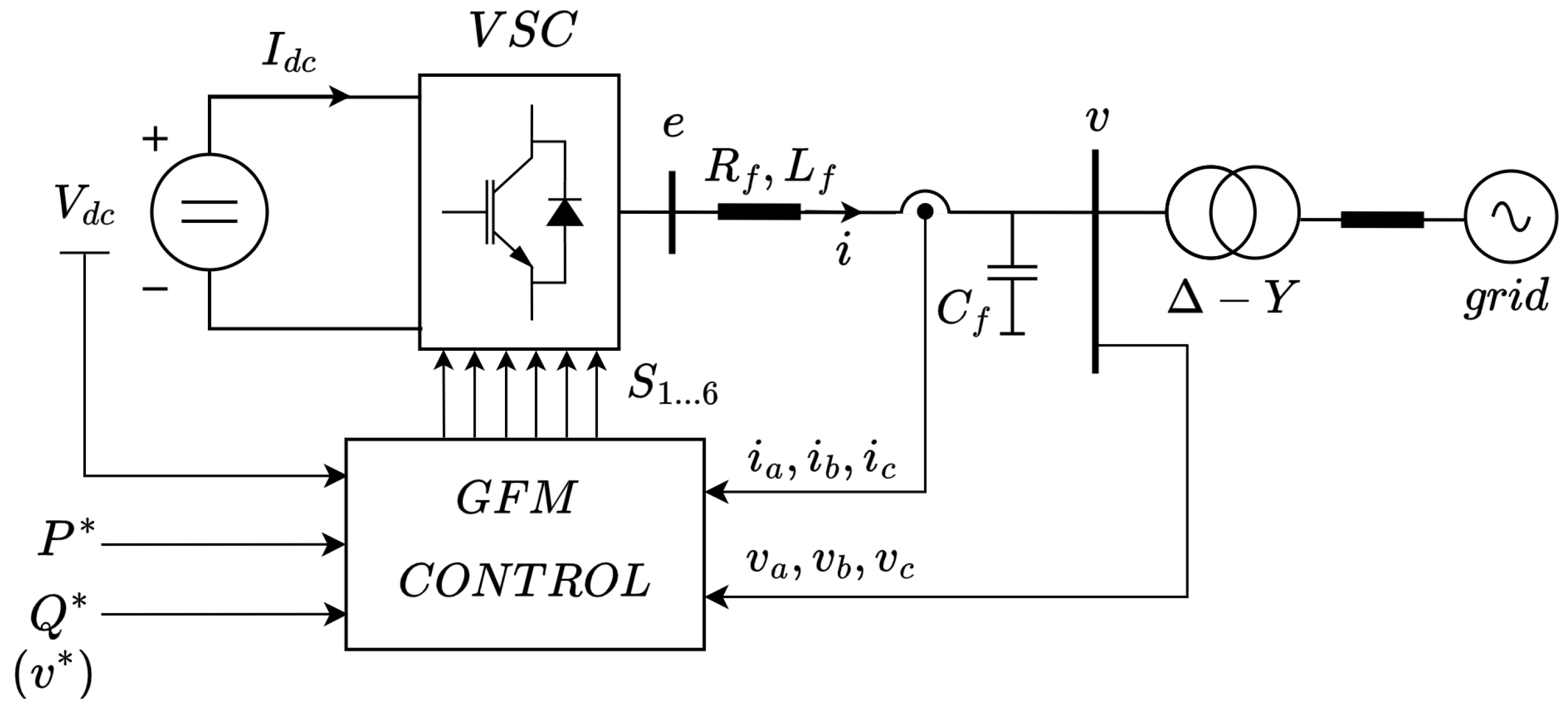
2. System Description and Virtual Flux Measurement
3. Control Schemes
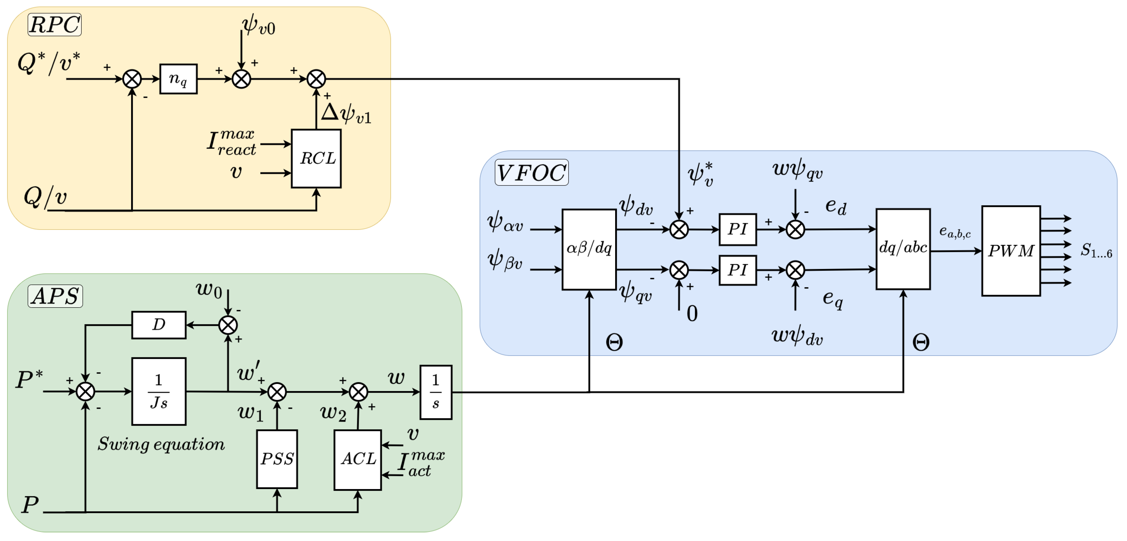
3.1. Virtual Flux-Oriented Control
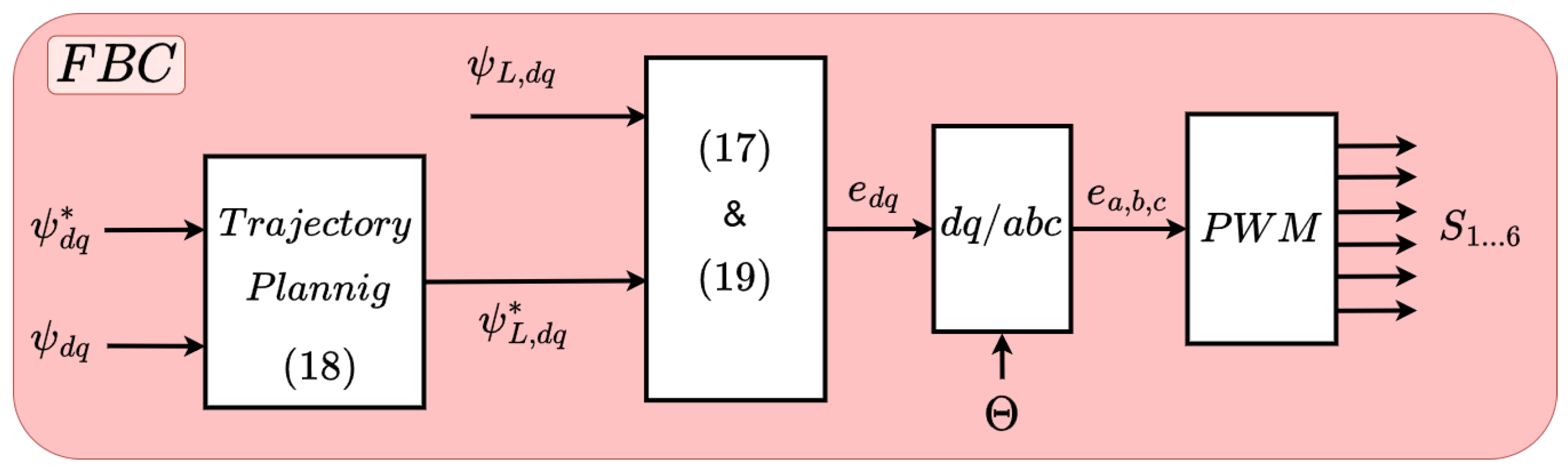
3.2. Flatness-Based Control
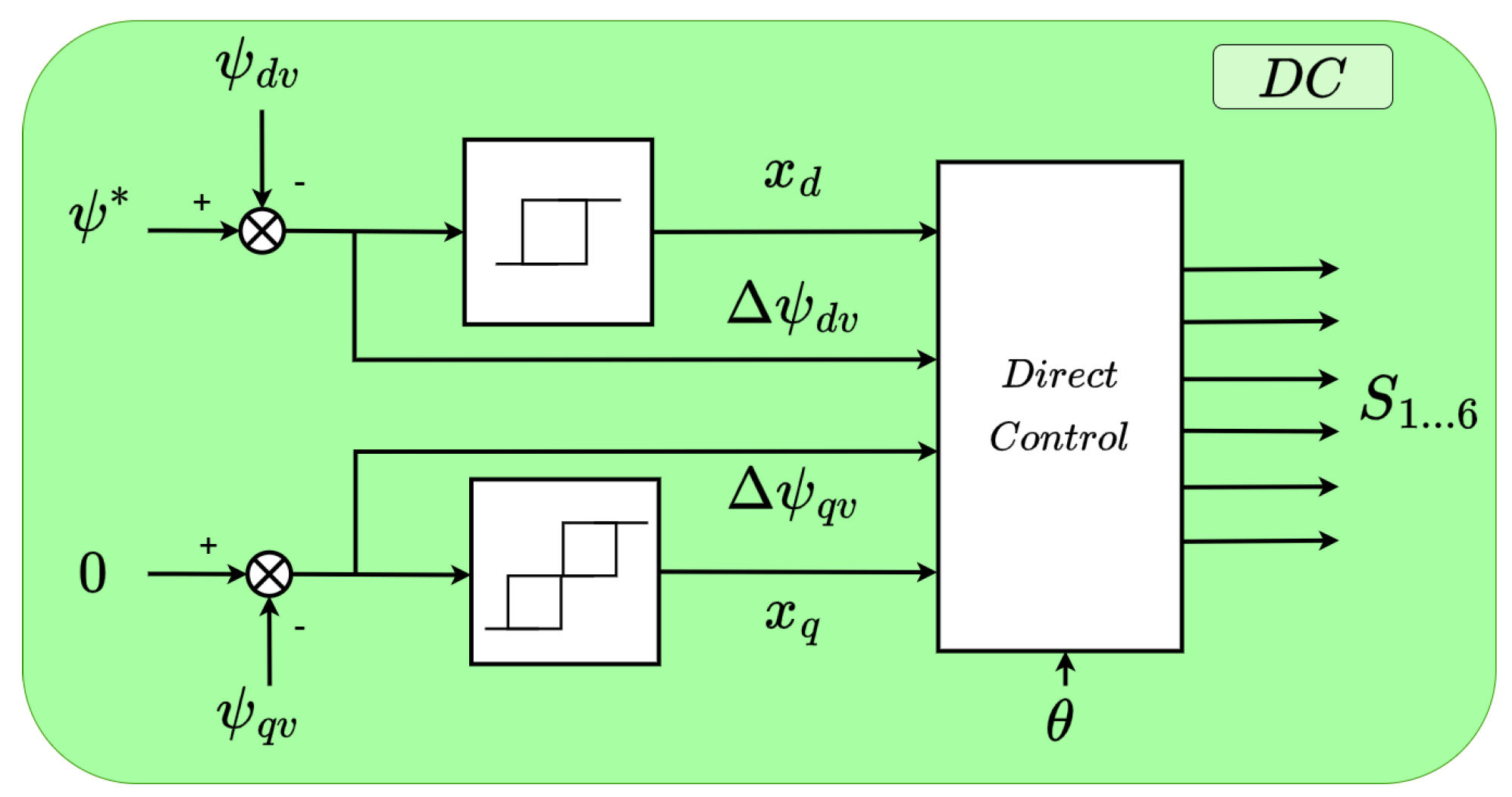
3.3. Direct Control
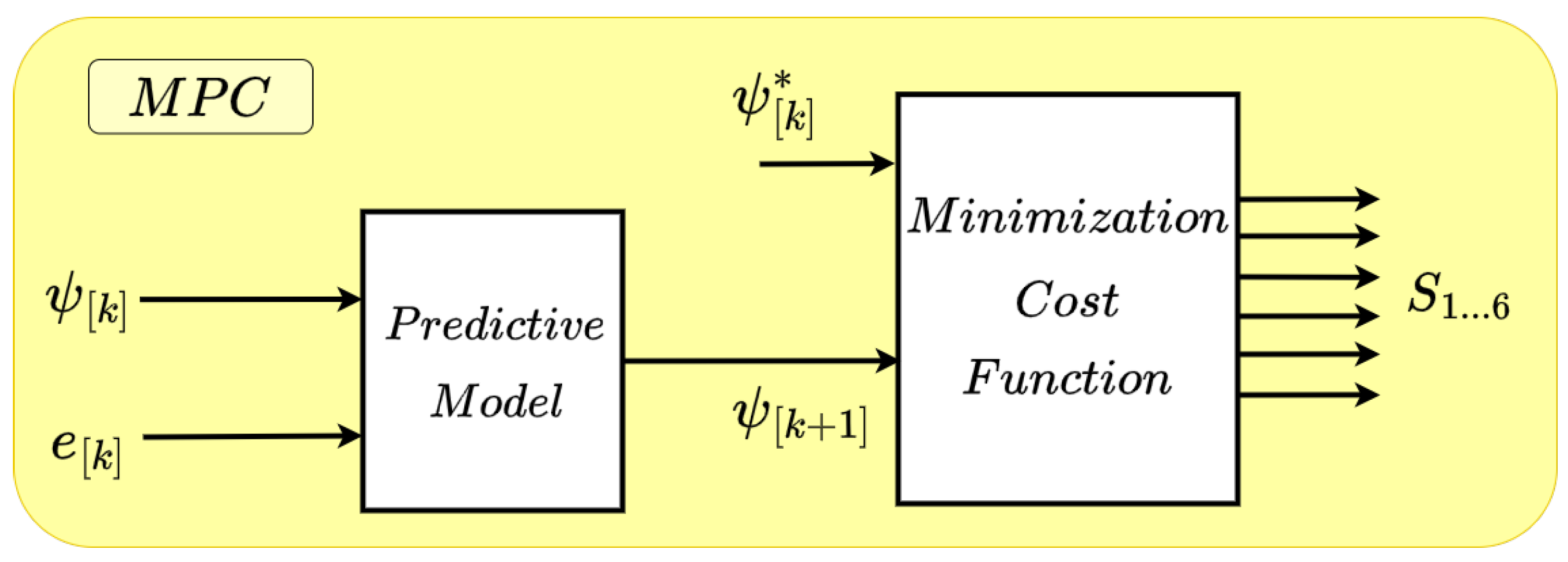
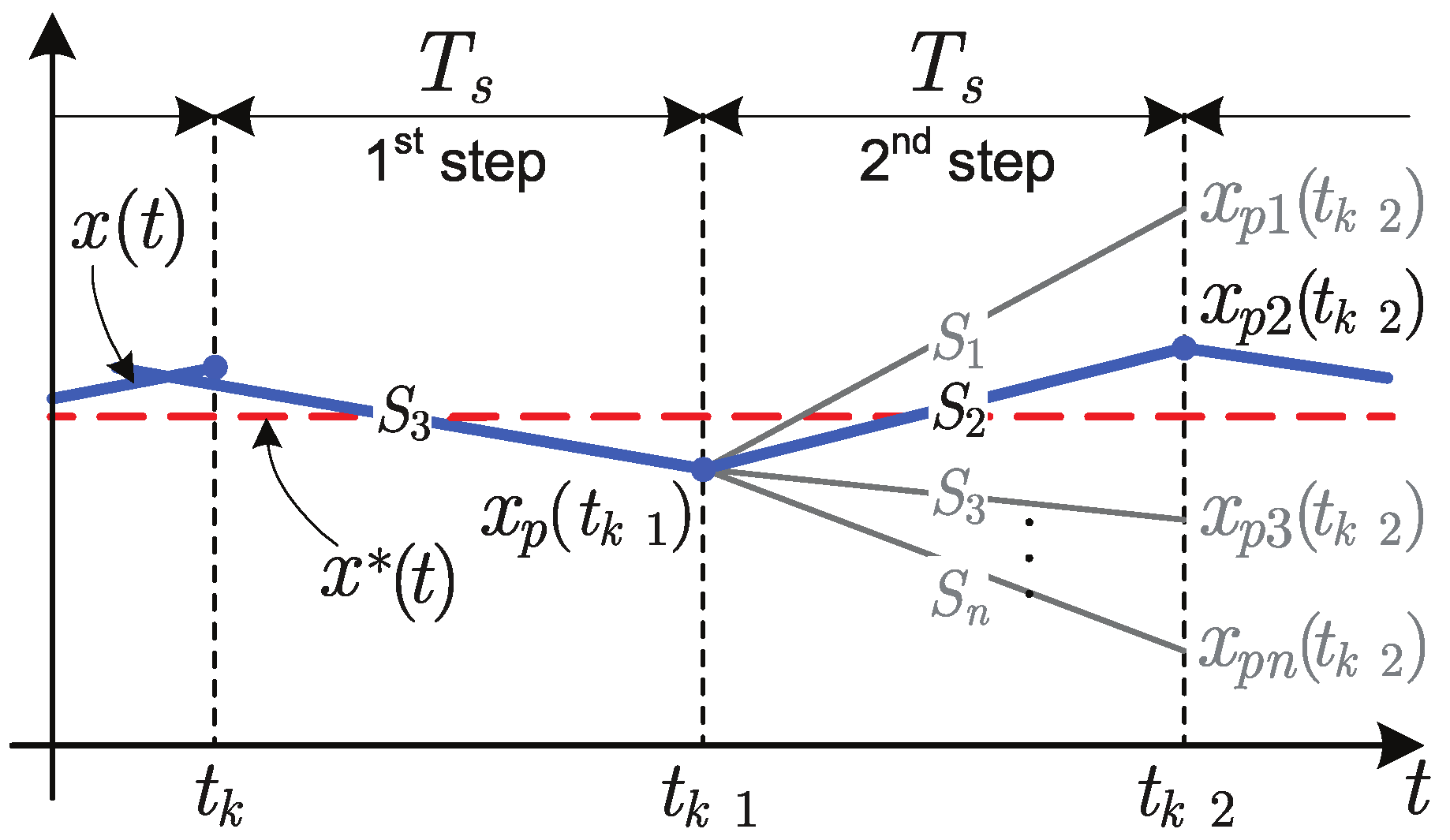
3.4. Model Predictive Control
4. HIL Results and Comparison
- Reactive Power Capability: GFM units must be capable of both generating and absorbing reactive power.
- Voltage Regulation: GFM converters are expected to maintain control over their internal voltage vector, both in magnitude and angle, regardless of grid or load conditions.
- Active Power Control: These converters must emulate the behavior of synchronous machines, supplying active power in response to control setpoints.
- Frequency Support: GFM units should respond to frequency deviations by adjusting their active power output, thereby contributing to system frequency stability.
- Damping of Oscillations: PSS or equivalent mechanisms are encouraged to mitigate low-frequency oscillations. In this case, prior validation has been conducted by the authors using Hardware-in-the-Loop simulations [62].
- Fault Ride Through and Dynamic Current Injection: GFM converters must remain connected during grid faults and must be able to inject reactive current rapidly to support voltage recovery.
- ROCOF Response: These units must be able to provide inertial response by injecting active power during periods of high rate of change of frequency (ROCOF), in addition to regular frequency support.
- Phase Jump Response: In events involving sudden phase angle changes between the converter and the grid, the system must manage transient power exchanges to maintain stability.
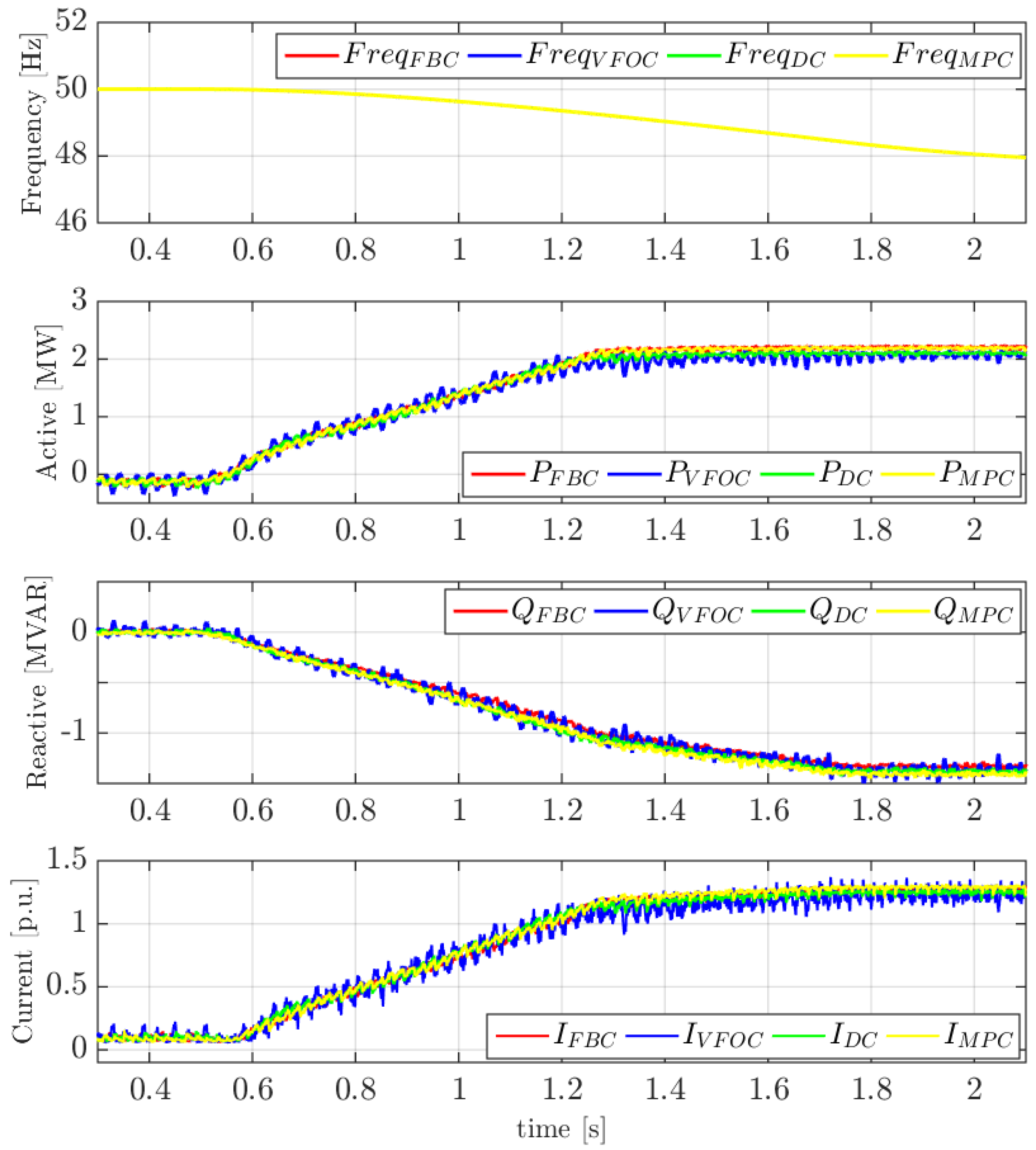
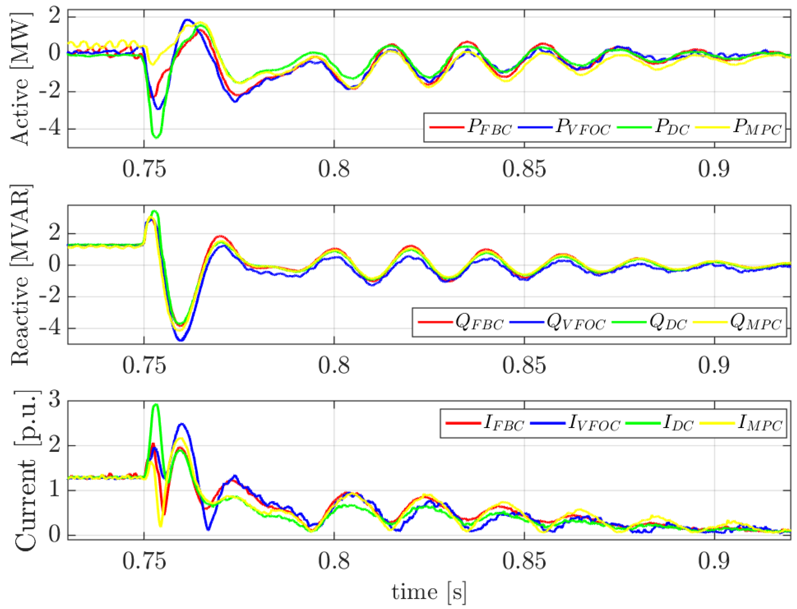
4.1. Frequency Variation
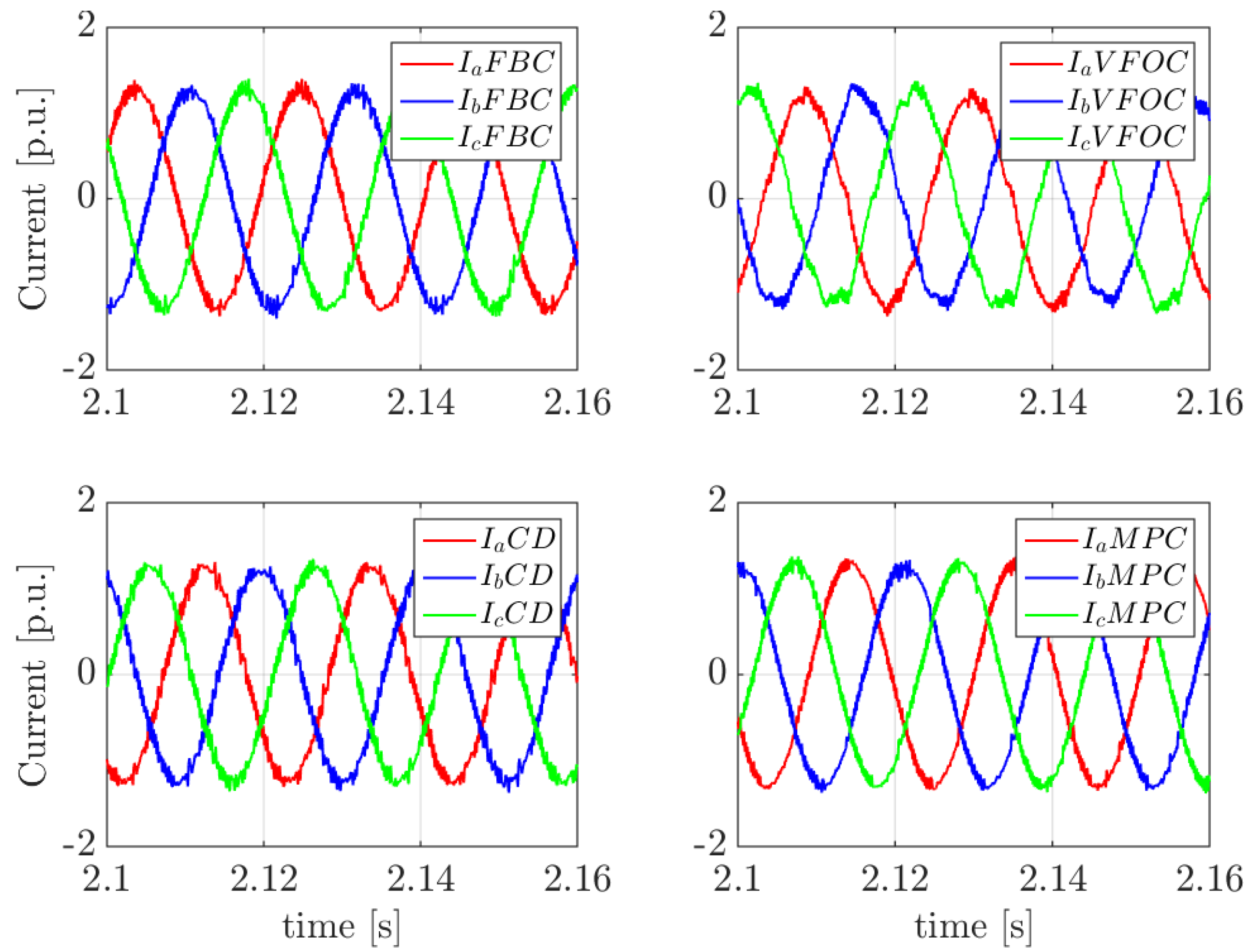
4.2. Phase Jump
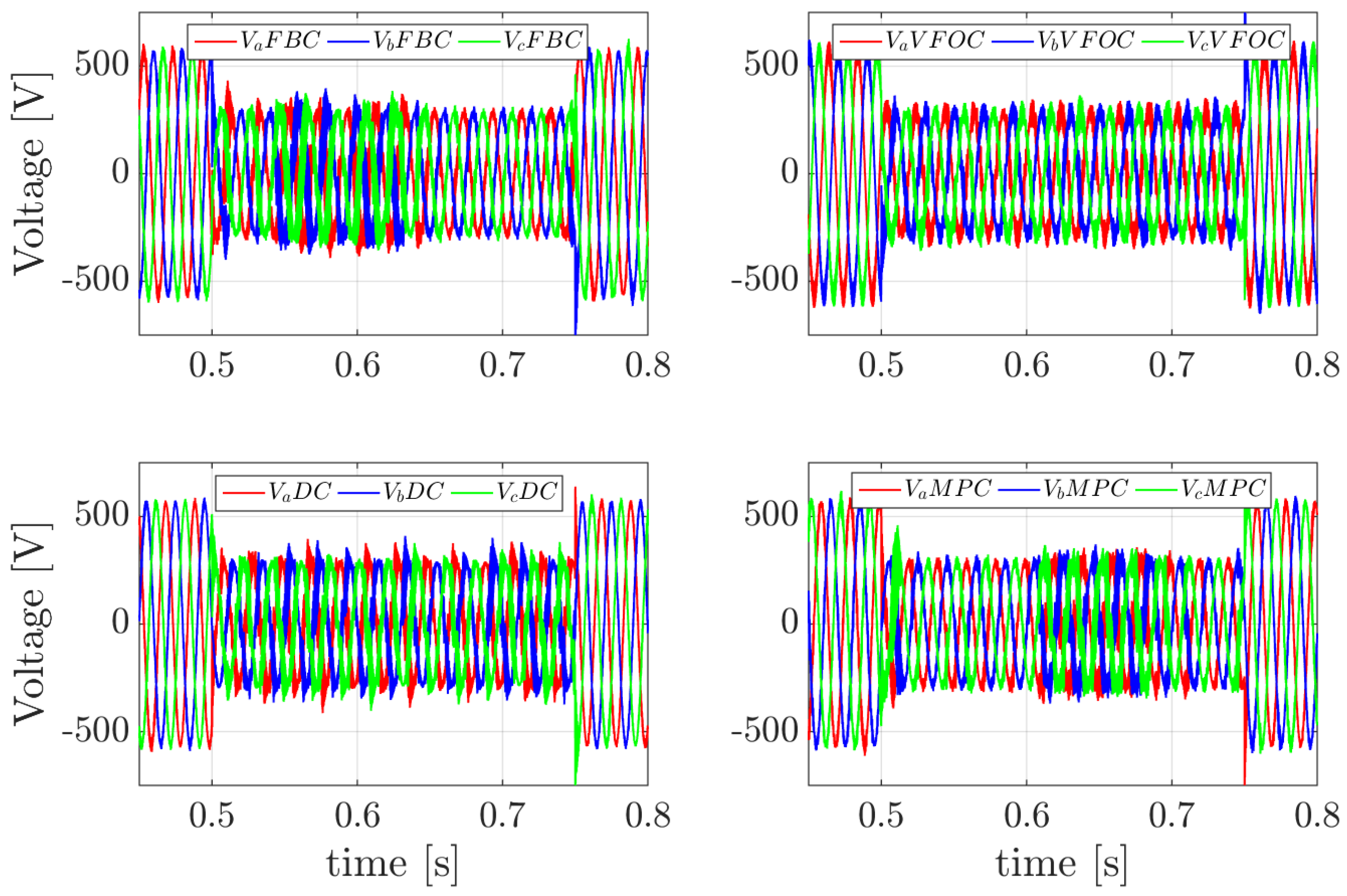
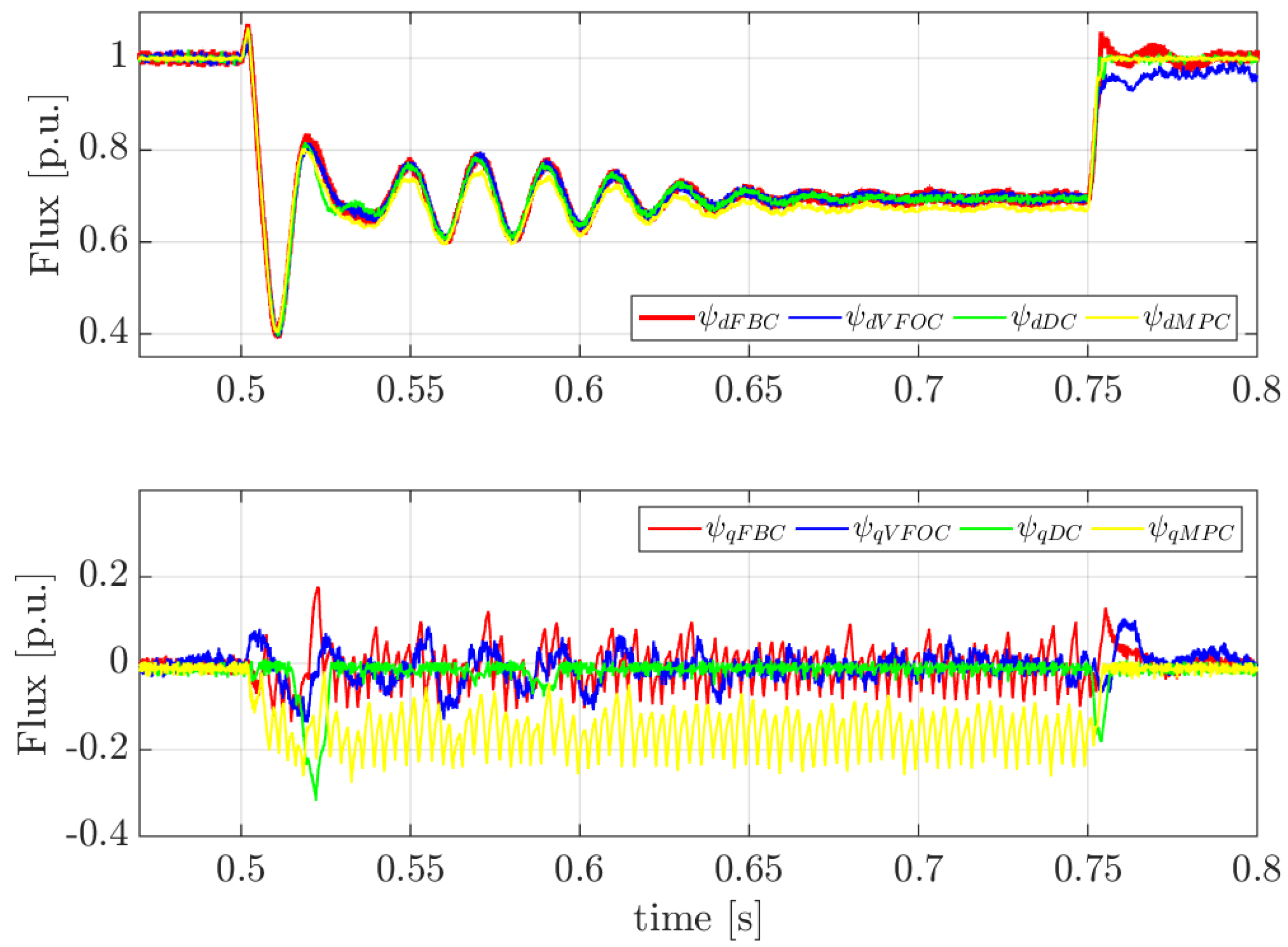
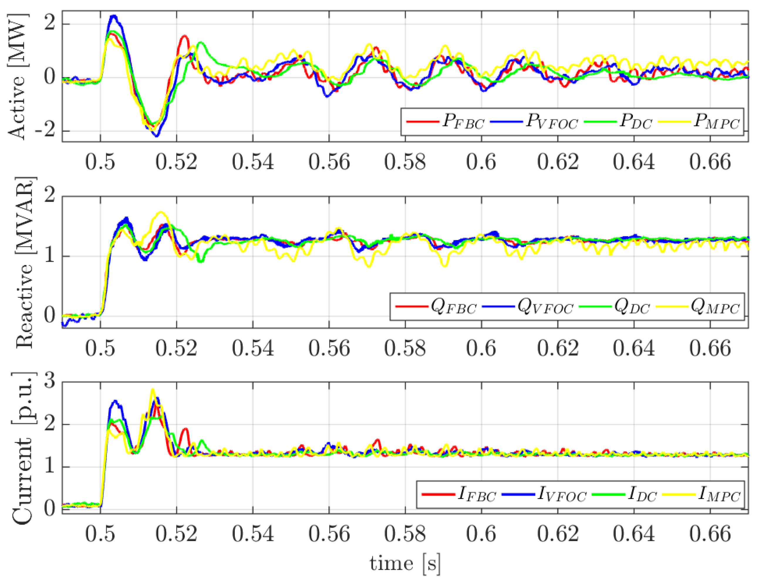
4.3. Low Voltage Ride-Through
4.4. Islanded Mode Operation
4.5. Switching Frequency Comparison
5. Discusion and Conclusions
Author Contributions
Funding
Institutional Review Board Statement
Informed Consent Statement
Data Availability Statement
Conflicts of Interest
Abbreviations
| ACL | Active Current Limiter; |
| APS | Active Power Synchronization; |
| DC | Direct Control; |
| ENTSO-E | European Network of Transmission System Operators for Electricity; |
| FBC | Flatness-Based Control; |
| FOC | Field-Oriented Controller; |
| GFL | Grid-following; |
| GFM | Grid-forming; |
| HIL | Hardware-in-the-Loop; |
| IBR | Inverter-Based Resources; |
| IRENA | International Renewable Energy Agency; |
| MPC | Model Predictive Control; |
| NESO | National Energy System Operator; |
| PSS | Power System Stabilizer; |
| PLL | Phase-Locked Loop; |
| PWM | Pulse Width Modulation; |
| RES | Renewable Energy Source; |
| RCL | Reactive Current Limiter; |
| ROCOF | Rate of Change of Frequency; |
| RPC | Reactive Power Controller; |
| SG | Synchronous Generator; |
| VFOC | Virtual-Flux Orientation Control; |
| VSC | Voltage Source Controller; |
| VOC | Virtual Oscillation-based Controller. |
Appendix A
Appendix A.1. System Parameters
| Parameter | Value | Units |
| DC voltage, | 1200 | V |
| Converter rated power, | 2 | MVA |
| Converter rated voltage (line to line), | 690 | V |
| Filter resistance, | 0.7104 | mΩ |
| Filter inductance, | 200 | μH |
| Filter capacitance, | 200 | μF |
| Nominal frequency, | 50 | Hz |
| Switching frequency, | 3000 | Hz |
Appendix A.2. Control System Parameters
| Parameter | Value | Units |
| Damping constant, D | 50 | p.u. |
| Inertia constant, H | 3.5 | s |
| PSS time constant, | 1.2 | s |
| PSS constant, | 0.01 | p.u. |
| RCL gain, | 0.15 | p.u. |
| RCL gain, | 0.15 | p.u. |
| Damping factor, | 0.7 | p.u. |
| Natural frequency, | 2000 | rad/s |
References
- International Renewable Energy Agency (IRENA). Renewable Energy Statistics. 2021. ISBN: 978-92-9260-356-4. Available online: https://www.irena.org/-/media/Files/IRENA/Agency/Publication/2021/Aug/IRENA_Renewable_Energy_Statistics_2021.pdf (accessed on 1 May 2025).
- Christensen, P.; Andersen, G.K.; Seidel, M.; Bolik, S.; Engelken, S.; Knueppel, T.; Krontiris, A.; Wuerflinger, K.; Bülo, T.; Jahn, J.; et al. High Penetration of Power Electronic Interfaced Power Sources and the Potential Contribution of Grid Forming Converters; ENTSO-E 2020; ENTSO: Brussels, Belgium, 2020. [Google Scholar]
- Zarei, S.F.; Mokhtari, H.; Ghasemi, M.A.; Blaabjerg, F. Reinforcing Fault Ride Through Capability of Grid Forming Voltage Source Converters Using an Enhanced Voltage Control Scheme. IEEE Trans. Power Deliv. 2019, 34, 1827–1842. [Google Scholar] [CrossRef]
- Zhang, Q.; Mao, M.; Ke, G.; Zhou, L.; Xie, B. Stability problems of PV inverter in weak grid: A review. IET Power Electron. 2020, 13, 2165–2174. [Google Scholar] [CrossRef]
- Li, Y.; Gu, Y.; Green, T.C. Revisiting Grid-Forming and Grid-Following Inverters: A Duality Theory. IEEE Trans. Power Syst. 2022, 37, 4541–4554. [Google Scholar] [CrossRef]
- Rosso, R.; Wang, X.; Liserre, M.; Lu, X.; Engelken, S. Grid-Forming Converters: Control Approaches, Grid-Synchronization, and Future Trends—A Review. IEEE Open J. Ind. Appl. 2021, 2, 93–109. [Google Scholar] [CrossRef]
- Wu, H.; Wang, X. Design-oriented transient stability analysis of PLL-synchronized voltage-source converters. IEEE Trans. Power Electron. 2020, 35, 3573–3589. [Google Scholar] [CrossRef]
- Tielens, P.; Van Hertem, D. The relevance of inertia in power systems. Renew. Sustain. Energy Rev. 2016, 55, 999–1009. [Google Scholar] [CrossRef]
- Matevosyan, J.; MacDowell, J.; Miller, N.; Badrzadeh, B.; Ramasubramanian, D.; Isaacs, A.; Quint, R.; Quitmann, E.; Pfeiffer, R.; Urdal, H.; et al. A future with inverter-based resources: Finding strength from traditional weakness. IEEE Power Energy Mag. 2021, 19, 18–29. [Google Scholar] [CrossRef]
- Zhang, L.; Harnefors, L.; Nee, H.-P. Power-synchronization control of grid-connected voltage-source converters. IEEE Trans. Power Syst. 2010, 25, 809–8200. [Google Scholar] [CrossRef]
- Anttila, S.; Döhler, J.S.; Oliveira, J.G.; Boström, C. Grid forming inverters: A review of the state of the art of key elements for microgrid operation. Energies 2022, 15, 5517. [Google Scholar] [CrossRef]
- Mohammed, N.; Udawatte, H.; Zhou, W.; Hill, D.J.; Bahrani, B. Grid-Forming Inverters: A Comparative Study of Different Control Strategies in Frequency and Time Domains. IEEE Open J. Ind. Electron. Soc. 2024, 5, 185–214. [Google Scholar] [CrossRef]
- Zhang, H.; Xiang, W.; Lin, W.; Wen, J. Grid forming converters in renewable energy sources dominated power grid: Control strategy, stability, application, and challenges. J. Mod. Power Syst. Clean Energy 2021, 9, 1239–1256. [Google Scholar] [CrossRef]
- Fazal, S.; Haque, M.E.; Arif, M.T.; Gargoom, A. Droop Control Techniques for Grid Forming Inverter. In Proceedings of the 2022 IEEE PES 14th Asia-Pacific Power and Energy Engineering Conference (APPEEC), Melbourne, Australia, 20–23 November 2022; pp. 1–6. [Google Scholar]
- Mohiuddin, S.M.; Qi, J. A Unified Droop-Free Distributed Secondary Control for Grid-Following and Grid-Forming Inverters in AC Microgrids. In Proceedings of the 2020 IEEE Power & Energy Society General Meeting (PESGM), Montreal, QC, Canada, 2–6 August 2020; pp. 1–5. [Google Scholar]
- Awal, M.A.; Yu, H.; Lukic, S.; Husain, I. Droop and Oscillator Based Grid-Forming Converter Controls: A Comparative Performance Analysis. Front. Energy Res. 2020, 8, 168. [Google Scholar] [CrossRef]
- Du, W.; Chen, Z.; Schneider, K.P.; Lasseter, R.H.; Nandanoori, S.P.; Tuffner, F.K.; Kundu, S. A Comparative Study of Two Widely Used Grid-Forming Droop Controls on Microgrid Small-Signal Stability. IEEE J. Emerg. Sel. Top. Power Electron. 2020, 8, 963–975. [Google Scholar] [CrossRef]
- Unruh, P.; Nuschke, M.; Strauß, P.; Welck, F. Overview on Grid-Forming Inverter Control Methods. Energies 2020, 13, 2589. [Google Scholar] [CrossRef]
- Li, D.; Zhu, Q.; Lin, S.; Bian, X.Y. A self-adaptive inertia and damping combination control of VSG to support frequency stability. IEEE Trans. Energy Convers. 2017, 32, 397–398. [Google Scholar] [CrossRef]
- Ashabani, M.; Jung, J. Synchronous voltage controllers: Voltage-based emulation of synchronous machines for the integration of renewable energy sources. IEEE Access 2020, 8, 49497–49508. [Google Scholar] [CrossRef]
- Bevrani, H.; Ise, T.; Miura, Y. Virtual synchronous generators: A survey and new perspectives. Electr. Power Syst. Res. 2014, 54, 244–254. [Google Scholar] [CrossRef]
- Li, M.; Huang, W.; Tai, N.; Yang, L.; Duan, D.; Ma, Z. A dual-adaptivity inertia control strategy for virtual synchronous generator. IEEE Trans. Power Syst. 2020, 35, 594–604. [Google Scholar] [CrossRef]
- Colombino, M.; Groß, D.; Brouillon, J.; Dörfler, F. Global phase and magnitude synchronization of coupled oscillators with application to the control of grid-forming power inverters. IEEE Trans. Autom. Control 2019, 64, 4496–45119. [Google Scholar] [CrossRef]
- Yu, M.; Roscoe, A.J.; Booth, C.D.; Dysko, A.; Ierna, R.; Zhu, J.; Grid, N.; Urdal, H. Use of an inertia-less virtual synchronous machine within future power networks with high penetrations of converters. In Proceedings of the 2016 Power Systems Computation Conference, Genoa, Italy, 20–24 June 2016. [Google Scholar]
- Sinha, M.; Dörfler, F.; Johnson, B.B.; Dhople, S.V. Uncovering droop control laws embedded within the nonlinear dynamics of van der pol oscillators. IEEE Trans. Control Netw. Syst. 2017, 4, 347–3587. [Google Scholar] [CrossRef]
- Awal, M.A.; Yu, H.; Tu, H.; Lukic, S.M.; Husain, I. Hierarchical control for virtual oscillator based grid-connected and islanded microgrids. IEEE Trans. Power Electron. 2020, 35, 988–1001. [Google Scholar] [CrossRef]
- Johnson, B.B.; Sinha, M.; Ainsworth, N.G.; Dörfler, F.; Dhople, S.V. Synthesizing virtual oscillators to control islanded inverters. IEEE Trans. Power Electron. 2016, 31, 6002–6015. [Google Scholar] [CrossRef]
- Awal, M.A.; Husain, I. Unified virtual oscillator control for gridforming and grid-following converters. IEEE J. Emerg. Sel. Topics Power Electron. 2021, 9, 4573–4586. [Google Scholar] [CrossRef]
- Azizi Aghdam, S.; Agamy, M. Virtual oscillator-based methods for grid-forming inverter control: A review. IET Renew. Power Gener. 2022, 16, 835–855. [Google Scholar] [CrossRef]
- Sadeque, F.; Fateh, F. On Control Schemes for Grid-Forming Inverters. In Proceedings of the IEEE Kansas Power and Energy Conference (KPEC), Manhattan, KS, USA, 25–26 April 2022; pp. 1–6. [Google Scholar]
- Nurunnabi, M.; Li, S.; Das, H.S. Control and Operation Evaluation of Grid-Forming Inverters with L, LC, and LCL Filters. In Proceedings of the 2023 IEEE Power & Energy Society General Meeting (PESGM), Orlando, FL, USA, 16–20 July 2023; pp. 1–5. [Google Scholar]
- Reißner, F.; Weiss, G. Robust and Adaptive Tuning of PI Current Controllers for Grid-Forming Inverters. IEEE Open J. Ind. Electron. Soc. 2025, 6, 115–129. [Google Scholar] [CrossRef]
- Qoria, T.; Gruson, F.; Colas, F.; Guillaud, X.; Debry, M.-S.; Prevost, T. Tuning of Cascaded Controllers for Robust Grid-Forming Voltage Source Converter. In Proceedings of the 2018 Power Systems Computation Conference (PSCC), Dublin, Ireland, 11–15 June 2018; pp. 1–7. [Google Scholar]
- Houari, A.; Renaudineau, H.; Martin, J.-P.; Pierfederici, S.; Meibody-Tabar, F. Flatness-Based Control of Three-Phase Inverter With Output LC Filter. IEEE Trans. Ind. Electron. 2012, 59, 2890–2897. [Google Scholar] [CrossRef]
- Gensior, A.; Woywode, O.; Rudolph, J.; Guldner, H. On differential flatness trajectory planning observers and stabilization for dc-dc converters. IEEE Trans. Circuits Syst. I Reg. Pap. 2006, 53, 2000–2010. [Google Scholar] [CrossRef]
- Renaudineau, H.; Lopez, D.; Flores-Bahamonde, F.; Kouro, S. Flatness-based control of a boost inverter for PV microinverter application. In Proceedings of the 2017 IEEE 8th International Symposium on Power Electronics for Distributed Generation Systems (PEDG), Florianopolis, Brazil, 17–20 April 2017; pp. 1–6. [Google Scholar]
- Mungporn, P.; Thounthong, P.; Sikkabut, S.; Yodwong, B.; Chunkag, V.; Kumam, P.; Bizon, N.; Nahid-Mobarakeh, B.; Pierfederici, S. Dynamics improvement of 3-phase inverter with output LC-filter by using differential flatness based control for grid connected applications. In Proceedings of the 2016 19th International Conference on Electrical Machines and Systems (ICEMS), Chiba, Japan, 13–16 November 2016; pp. 1–6. [Google Scholar]
- Alonso-Martínez, J.; Eloy-García, J.; Arnaltes, S. Direct power control of grid connected PV systems with three level NPC inverter. Sol. Energy 2010, 84, 1175–1186. [Google Scholar]
- Maissa, M.; Kouider, L. Direct power control technique for Grid-tied two levels VSI inverter fed by photovoltaic system. In Proceedings of the 2023 1st International Conference on Renewable Solutions for Ecosystems: Towards a Sustainable Energy Transition (ICRSEtoSET), Djelfa, Algeria, 6–8 May 2023; pp. 1–5. [Google Scholar]
- Kulikowski, K.; Sikorski, A. New DPC Look-Up Table Methods for Three-Level AC/DC Converter. IEEE Trans. Ind. Electron. 2016, 63, 7930–7938. [Google Scholar] [CrossRef]
- Kouro, S.; Cortes, P.; Vargas, R.; Ammann, U.; Rodriguez, J. Model Predictive Control—A Simple and Powerful Method to Control Power Converters. IEEE Trans. Ind. Electron. 2009, 56, 1826–1838. [Google Scholar] [CrossRef]
- Heydari, R.; Young, H.; Flores-Bahamonde, F.; Vaez-Zadeh, S.; Gonzalez-Castano, C.; Sabzevari, S.; Rodriguez, J. Model-Free Predictive Control of Grid-Forming Inverters With LCL Filters. IEEE Trans. Power Electron. 2022, 37, 9200–9211. [Google Scholar] [CrossRef]
- Kumar, D.; Kumar, C. Model Predictive Control of Isolated Three-Phase Four-Wire Grid Forming Converter. In Proceedings of the 2023 11th National Power Electronics Conference (NPEC), Guwahati, India, 14–16 December 2023; pp. 1–5. [Google Scholar]
- Cortés, P.; Kouro, S.; La Rocca, B.; Vargas, R.; Rodríguez, J.; Leon, J.I.; Vazquez, S.; Franquelo, L.G. Guidelines for weighting factors design in Model Predictive Control of power converters and drives. In Proceedings of the 2009 IEEE International Conference on Industrial Technology, Churchill, VIC, Australia, 10–13 February 2009; pp. 1–7. [Google Scholar]
- Pérez-Guzmán, R.E.; Rivera, M.; Vicencio, N.; Wheeler, P.W. Model-based Predictive Control in Three-Phase Inverters. In Proceedings of the 2020 IEEE International Conference on Industrial Technology (ICIT), Buenos Aires, Argentina, 26–28 February 2020; pp. 499–504. [Google Scholar]
- Aguirre, M.; Kouro, S.; Rojas, C.A.; Rodriguez, J.; Leon, J.I. Switching Frequency Regulation for FCS-MPC Based on a Period Control Approach. IEEE Trans. Ind. Electron. 2018, 65, 5764–5773. [Google Scholar] [CrossRef]
- Aguirre, M.; Kouro, S.; Rojas, C.A.; Vazquez, S. Enhanced Switching Frequency Control in FCS-MPC for Power Converters. IEEE Trans. Ind. Electron. 2021, 68, 2470–2479. [Google Scholar] [CrossRef]
- Zubiaga, M.; Cardozo, C.; Prevost, T.; Sanchez-Ruiz, A.; Olea, E.; Izurza, P.; Khan, S.H.; Arza, J. Enhanced TVI for Grid Forming VSC under Unbalanced Faults. Energies 2021, 14, 6168. [Google Scholar] [CrossRef]
- Oureilidis, K.O.; Demoulias, C.S. A fault clearing method in converter-dominated microgrids with conventional protection means. IEEE Trans. Power Electron. 2016, 31, 4628–4640. [Google Scholar] [CrossRef]
- Shi, K.; Song, W.; Xu, P.; Fang, Z.; Ji, Y. Low-voltage ride-through control strategy for a virtual synchronous generator based on smooth switching. IEEE Access 2017, 6, 2703–2711. [Google Scholar] [CrossRef]
- Huang, L.; Xin, H.; Wang, Z.; Zhang, L.; Wu, K.; Hu, J. Transient stability analysis and control design of droop-controlled voltage source converters considering current limitation. IEEE Trans. Smart Grid 2017, 10, 578–591. [Google Scholar] [CrossRef]
- Jiang, S.; Zhu, Y.; Xu, T.; Konstantinou, G. Current-Synchronization Control of Grid-Forming Converters for Fault Current Limiting and Enhanced Synchronization Stability. IEEE Trans. Power Electron. 2024, 39, 5271–5285. [Google Scholar] [CrossRef]
- Jiang, S.; Xu, T.; Konstantinou, G. Current Synchronization Loop for Enhanced Fault Tolerance and Fast Recovery in Grid-Forming Converters. In Proceedings of the IECON 2023—49th Annual Conference of the IEEE Industrial Electronics Society, Singapore, 16–19 October 2023; pp. 1–6. [Google Scholar]
- Lu, X.; Wang, J.; Guerrero, J.M.; Zhao, D. Virtual-impedance-based fault current limiters for inverter dominated ac microgrids. IEEE Trans. Smart Grid 2018, 9, 1599–1612. [Google Scholar] [CrossRef]
- Wang, X.; Li, Y.W.; Blaabjerg, F.; Loh, P.C. Virtualimpedance-based control for voltage-source and current-source converters. IEEE Trans. Power Electron. 2015, 30, 7019–70375. [Google Scholar] [CrossRef]
- Groß, D.; Dörfler, F. Projected grid-forming control for current-limiting of power converters. In Proceedings of the 2019 57th Annual Allerton Conference on Communication, Control and Computing (Allerton), Monticello, IL, USA, 24–27 September 2019; pp. 326–333. [Google Scholar]
- Rodríguez-Amenedo, J.L.; Gómez, S.A.; Zubiaga, M.; Izurza-Moreno, P.; Arza, J.; Fernández, J.D. Grid-Forming Control of Voltage Source Converters Based on the Virtual-Flux Orientation. IEEE Access 2023, 11, 10254–10274. [Google Scholar] [CrossRef]
- Fernández, J.D.; Navarro, E.R.; Amenedo, J.L.R.; Eloy-García, J.; Gómez, S.A. Operation of a Grid-Forming Converter Controlled by the Flux Vector. IEEE Access 2025, 13, 7040–7052. [Google Scholar] [CrossRef]
- NGESO: Grid Forming Best Practice Grid. April 2023. Available online: https://www.neso.energy/document/278491/download (accessed on 31 January 2025).
- NGESO, GC0137: Minimum Specification Required for Provision of GB Grid Forming (GBGF) Capability. 2021. Available online: https://www.neso.energy/document/220511/download (accessed on 5 April 2025).
- Fliess, M.; Lévine, J.; Martin, P.; Rouchon, P. Flatness and defect of non-linear systems: Introductory theory and examples. Int. J. Control 1995, 61, 1327–1361. [Google Scholar] [CrossRef]
- Dolado, J.; Rodríguez Amenedo, J.L.; Arnaltes, S.; Eloy-Garcia, J. Improving the Inertial Response of a Grid-Forming Voltage Source Converter. Electronics 2022, 11, 2303. [Google Scholar] [CrossRef]
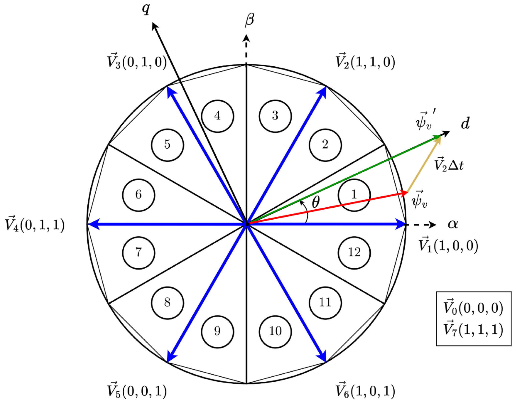


| Output | Sector | |||||||||||||
|---|---|---|---|---|---|---|---|---|---|---|---|---|---|---|
| Error | 1 | 2 | 3 | 4 | 5 | 6 | 7 | 8 | 9 | 10 | 11 | 12 | ||
| 1 | 1 | |||||||||||||
| 1 | 0 | |||||||||||||
| 1 | −1 | |||||||||||||
| −1 | 1 | |||||||||||||
| −1 | 0 | |||||||||||||
| 0 | 0 | 0 | |
| 1 | 0 | 0 | |
| 1 | 1 | 0 | |
| 0 | 1 | 0 | |
| 0 | 1 | 1 | |
| 0 | 0 | 1 | |
| 1 | 0 | 1 | |
| 1 | 1 | 1 |
| Method | Block Diagram | Inertial Respone & ACL | Phase Jump | Sag Entry & RCL | Sag Exit | Islanded Mode | |
|---|---|---|---|---|---|---|---|
| Virtual Flux-Oriented Control | 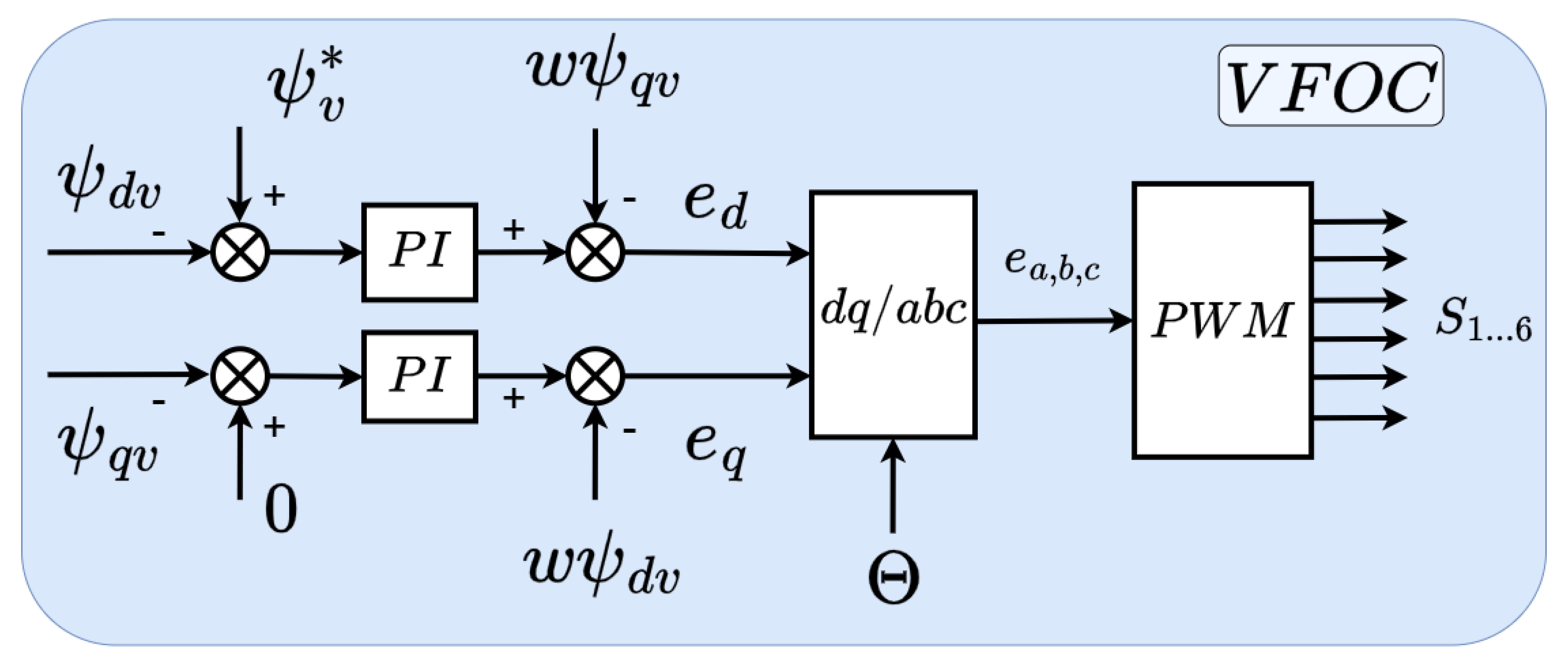 | ✓✓ | ✗✗ | ✓ | ✗ | ✓✓ | ✓✓ |
| Flatness-Based Control | 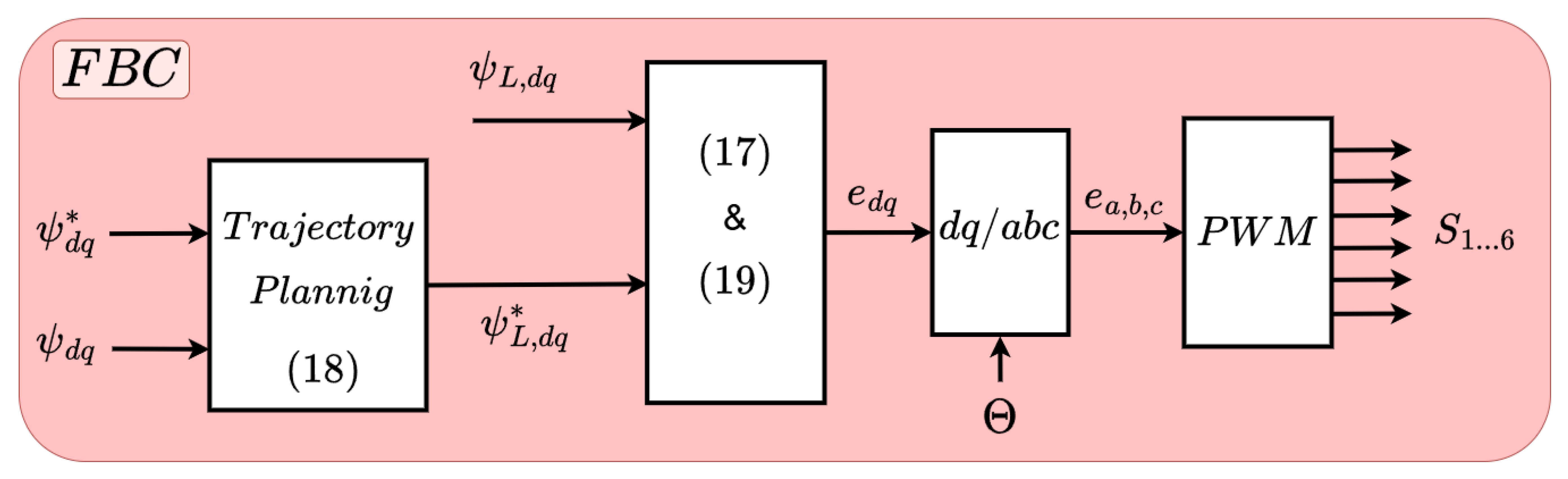 | ✓✓ | ✓✓ | ✗✗ | ✓✓ | ✓✓ | ✓✓ |
| Direct Control | 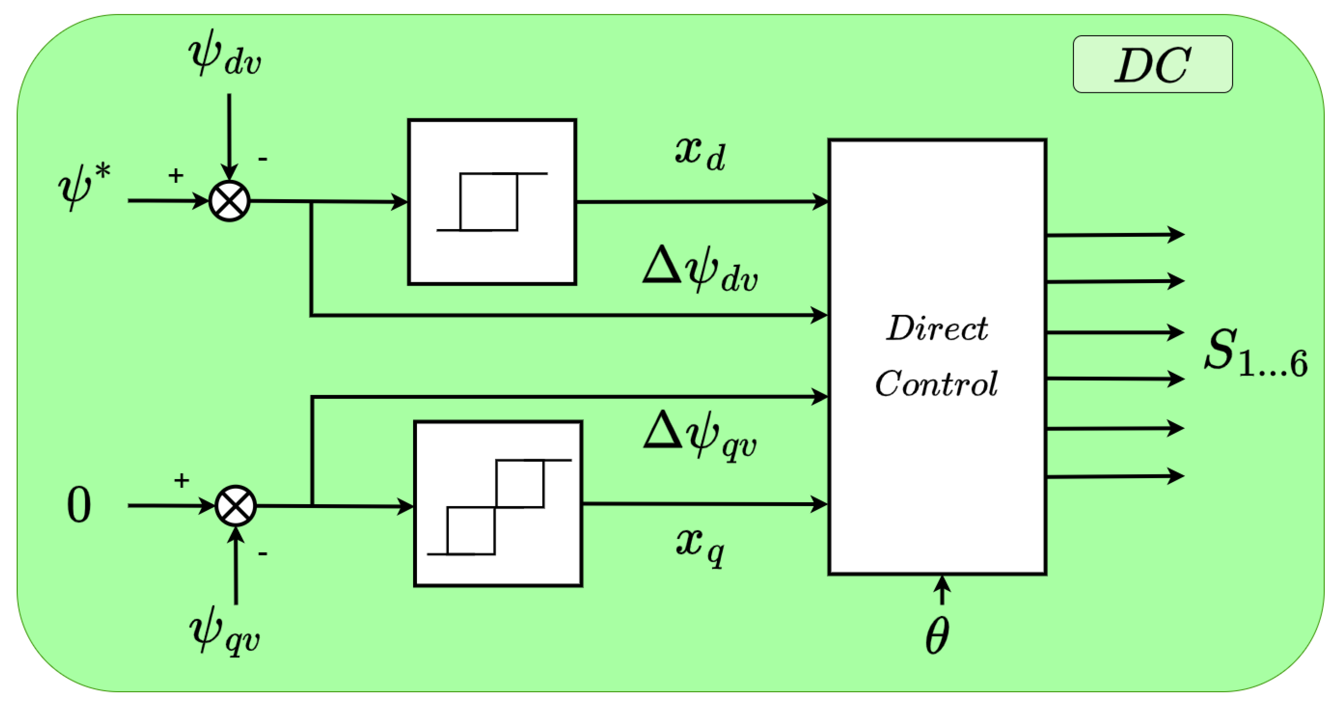 | ✓✓ | ✗ | ✓✓ | ✗✗ | ✓✓ | ✗ |
| Model Predictive Control |  | ✓✓ | ✓ | ✗✗ | ✓ | ✓✓ | ✗✗ |
Disclaimer/Publisher’s Note: The statements, opinions and data contained in all publications are solely those of the individual author(s) and contributor(s) and not of MDPI and/or the editor(s). MDPI and/or the editor(s) disclaim responsibility for any injury to people or property resulting from any ideas, methods, instructions or products referred to in the content. |
© 2025 by the authors. Licensee MDPI, Basel, Switzerland. This article is an open access article distributed under the terms and conditions of the Creative Commons Attribution (CC BY) license (https://creativecommons.org/licenses/by/4.0/).
Share and Cite
Dolado Fernández, J.; Eloy-García, J.; Arnaltes Gómez, S.; Kouro, S.; Renaudineau, H.; Rodríguez Amenedo, J.L. Virtual Flux Control Methods for Grid-Forming Converters: A Four-Method Comparison. Appl. Sci. 2025, 15, 5157. https://doi.org/10.3390/app15095157
Dolado Fernández J, Eloy-García J, Arnaltes Gómez S, Kouro S, Renaudineau H, Rodríguez Amenedo JL. Virtual Flux Control Methods for Grid-Forming Converters: A Four-Method Comparison. Applied Sciences. 2025; 15(9):5157. https://doi.org/10.3390/app15095157
Chicago/Turabian StyleDolado Fernández, Juan, Joaquín Eloy-García, Santiago Arnaltes Gómez, Samir Kouro, Hugues Renaudineau, and José Luis Rodríguez Amenedo. 2025. "Virtual Flux Control Methods for Grid-Forming Converters: A Four-Method Comparison" Applied Sciences 15, no. 9: 5157. https://doi.org/10.3390/app15095157
APA StyleDolado Fernández, J., Eloy-García, J., Arnaltes Gómez, S., Kouro, S., Renaudineau, H., & Rodríguez Amenedo, J. L. (2025). Virtual Flux Control Methods for Grid-Forming Converters: A Four-Method Comparison. Applied Sciences, 15(9), 5157. https://doi.org/10.3390/app15095157