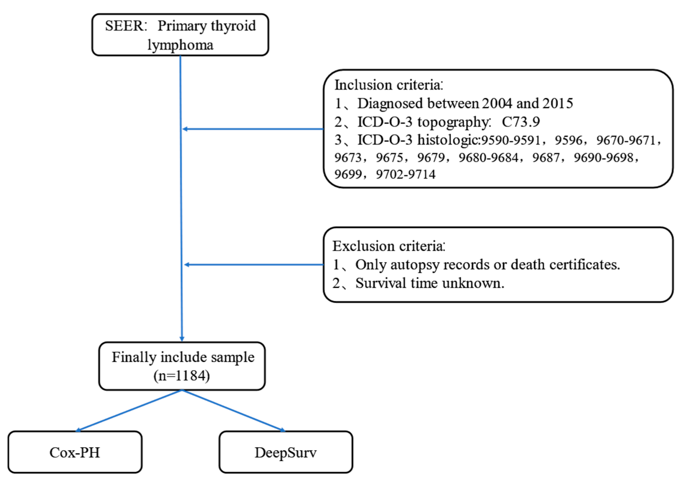
Figure 1.
Flow chart of PTL patient data selection in SEER database.
Figure 1.
Flow chart of PTL patient data selection in SEER database.
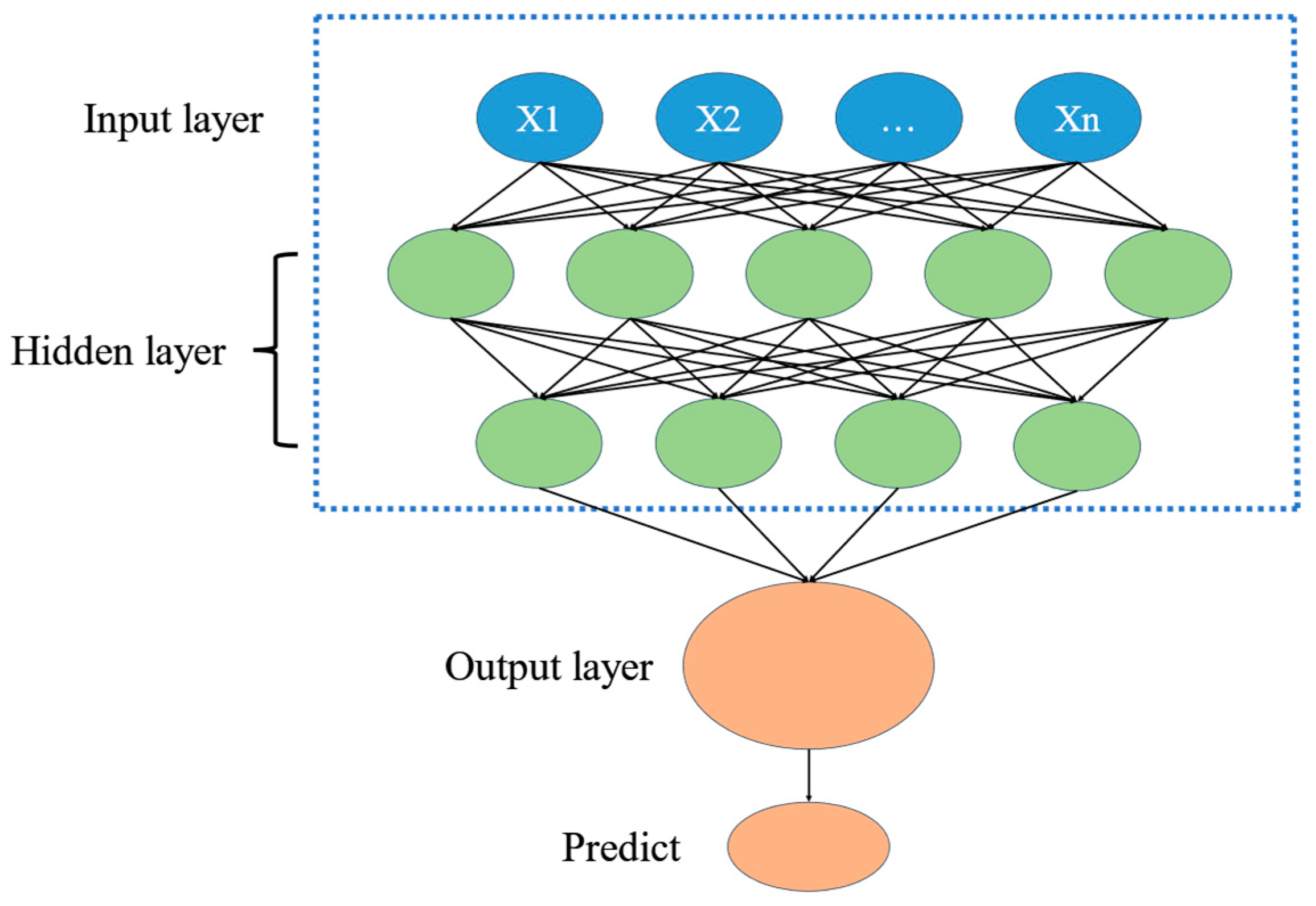
Figure 2.
Deep learning process diagram.
Figure 2.
Deep learning process diagram.
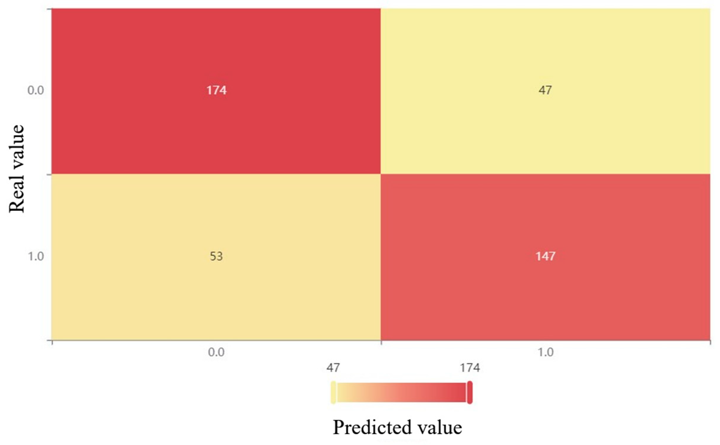
Figure 3.
XGBoost confusion matrix after oversampling.
Figure 3.
XGBoost confusion matrix after oversampling.
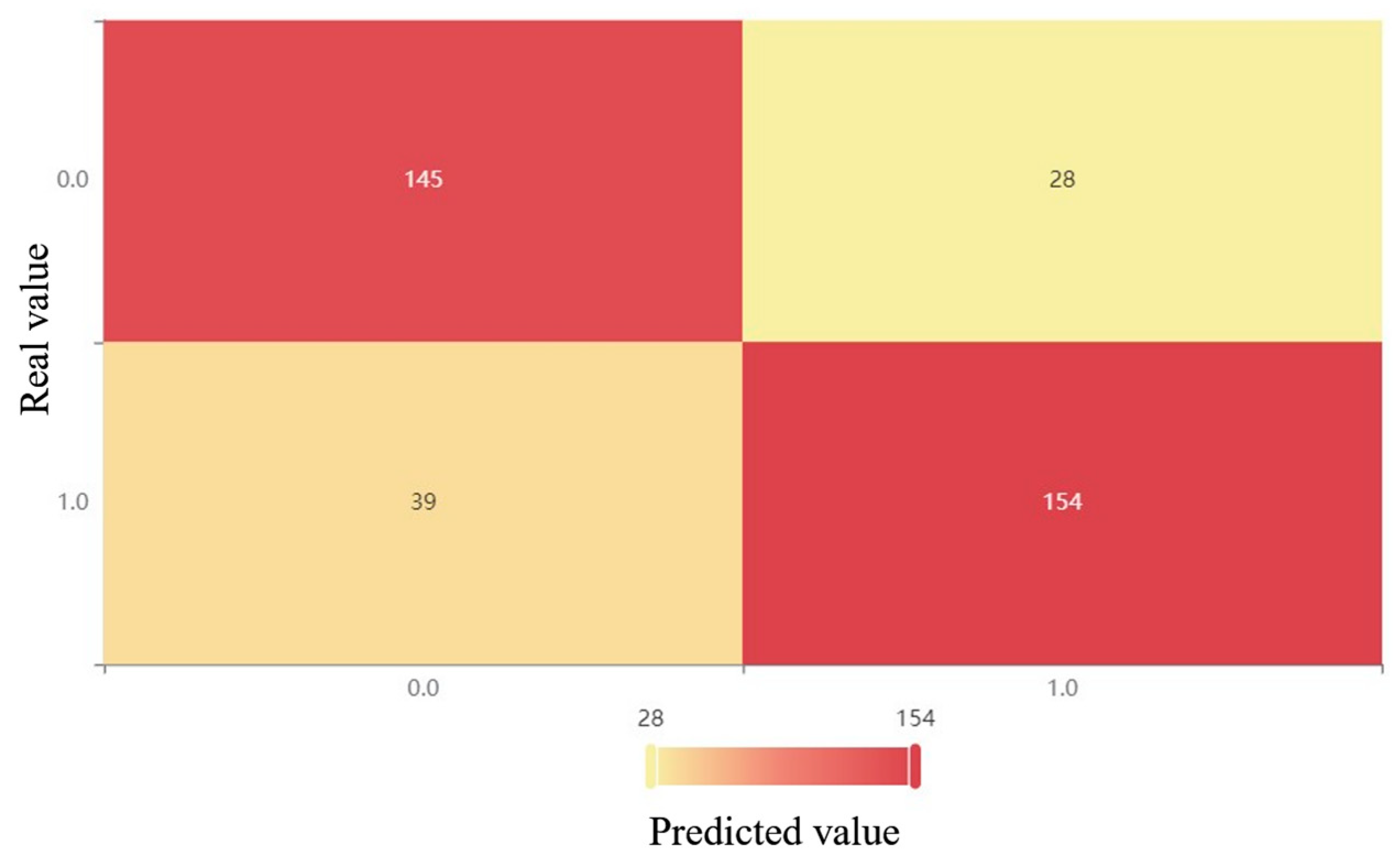
Figure 4.
XGBoost confusion matrix after downsampling.
Figure 4.
XGBoost confusion matrix after downsampling.
Figure 5.
XGBoost confusion matrix after combinatorial sampling.
Figure 5.
XGBoost confusion matrix after combinatorial sampling.
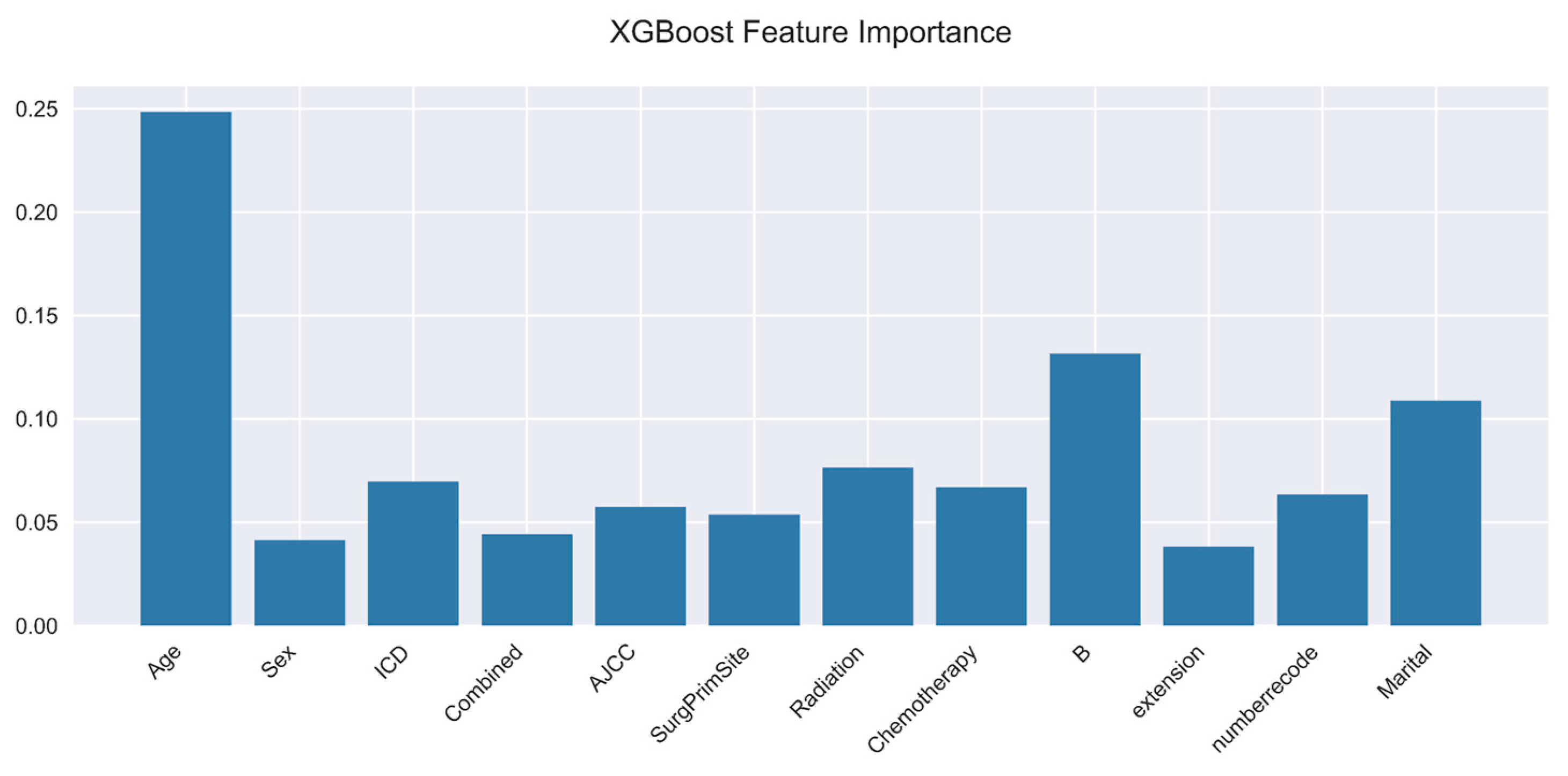
Figure 6.
XGBoost feature importance.
Figure 6.
XGBoost feature importance.
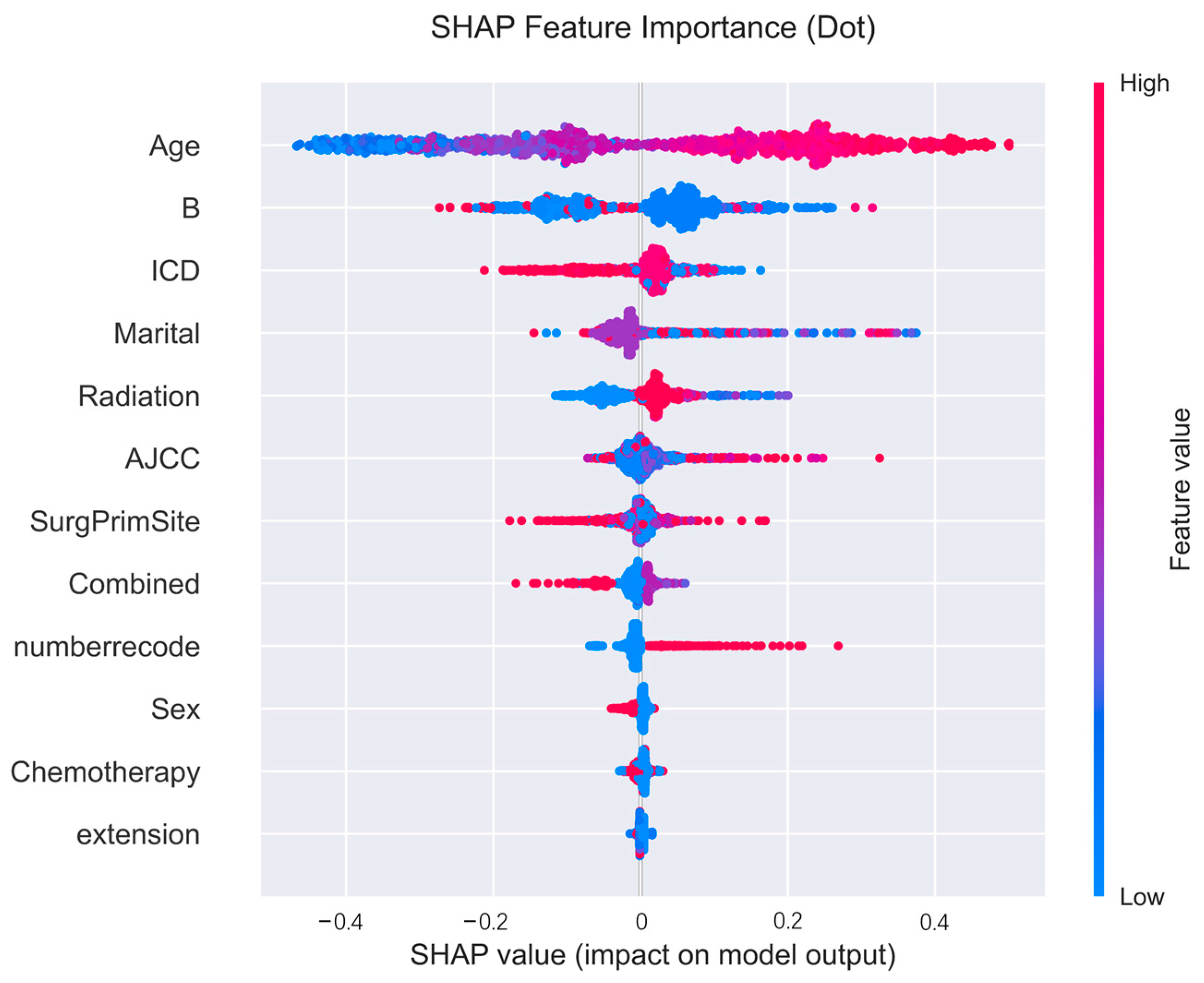
Figure 7.
Positive and negative effect plots for each variable in the SHAP framework.
Figure 7.
Positive and negative effect plots for each variable in the SHAP framework.
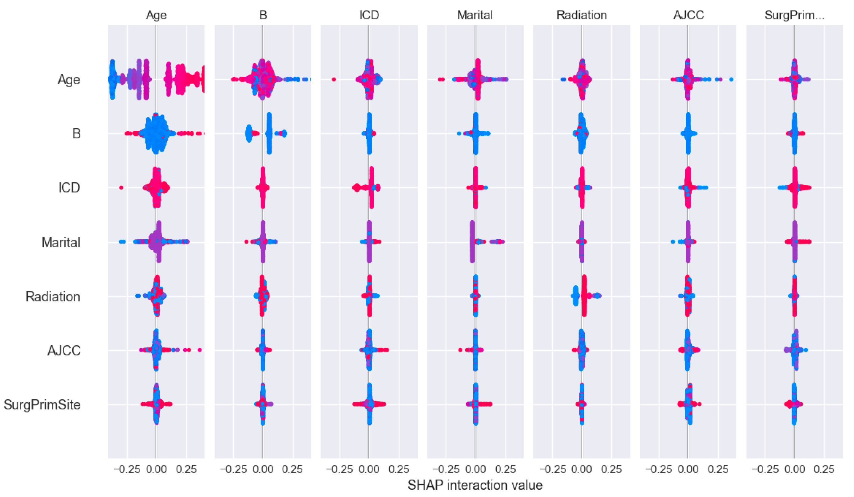
Figure 8.
The impact of two-by-two interaction characteristics on prediction outcomes.
Figure 8.
The impact of two-by-two interaction characteristics on prediction outcomes.
Figure 9.
Decision charts for the first 100 patients.
Figure 9.
Decision charts for the first 100 patients.
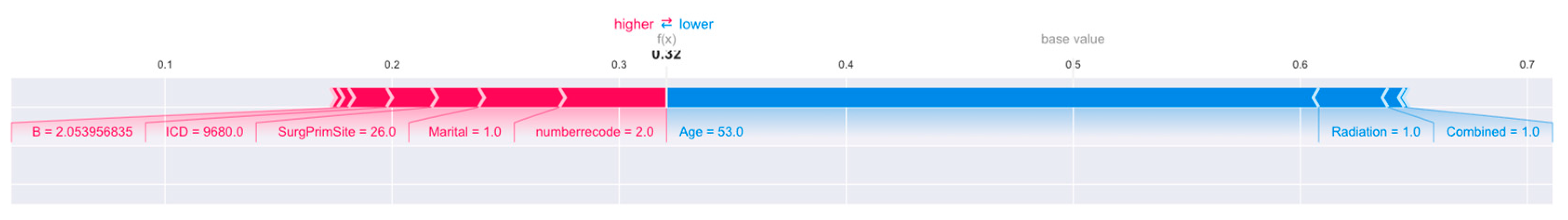
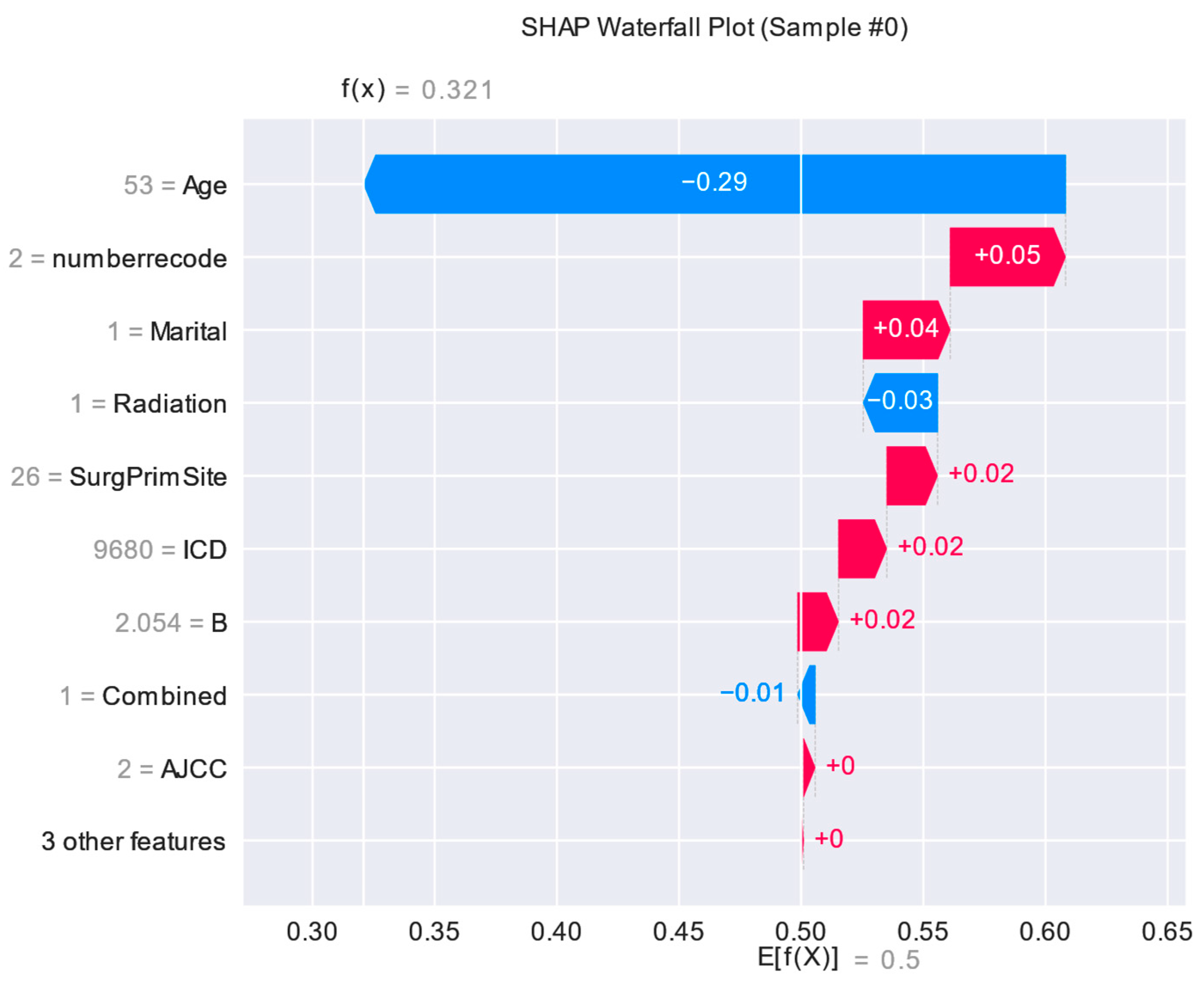
Figure 10.
Interpretation of the SHAP model for the 30th patient.
Figure 10.
Interpretation of the SHAP model for the 30th patient.
Figure 11.
Importance of characteristics of 30th patient.
Figure 11.
Importance of characteristics of 30th patient.
Figure 12.
Multivariate cox regression analysis.
Figure 12.
Multivariate cox regression analysis.
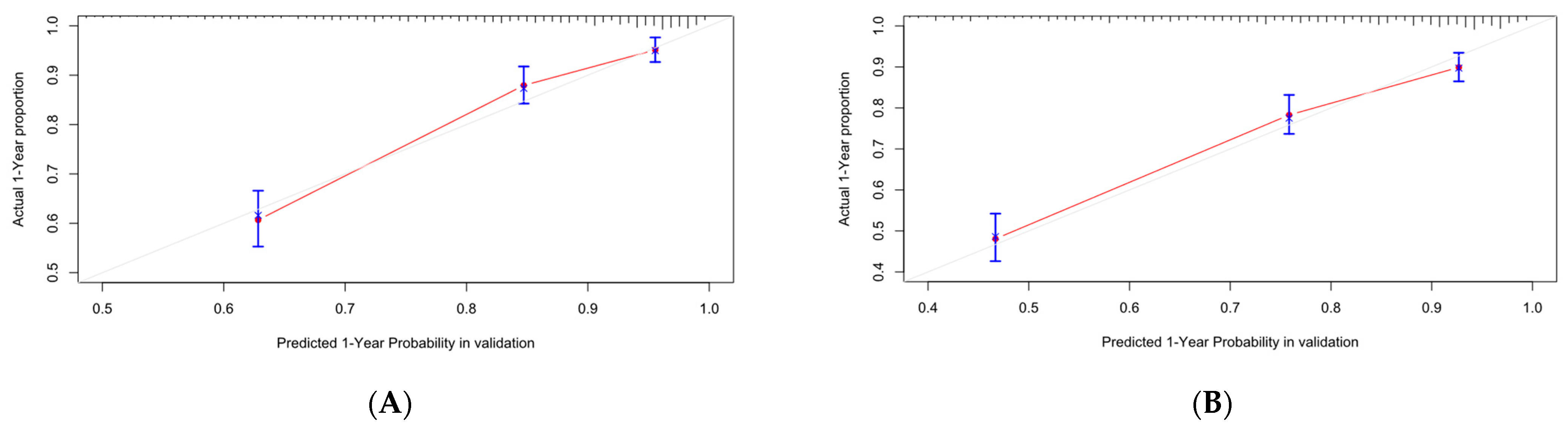
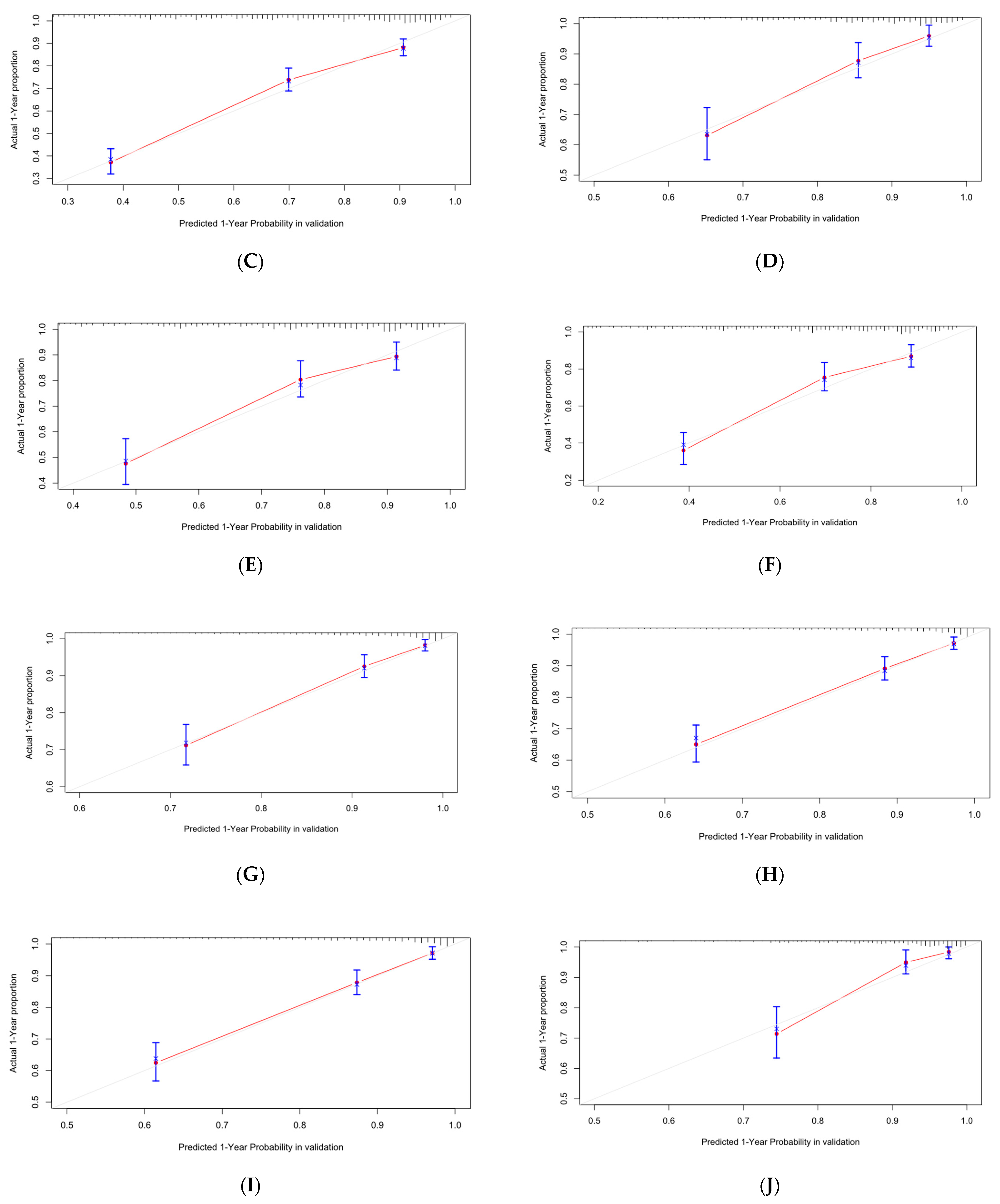
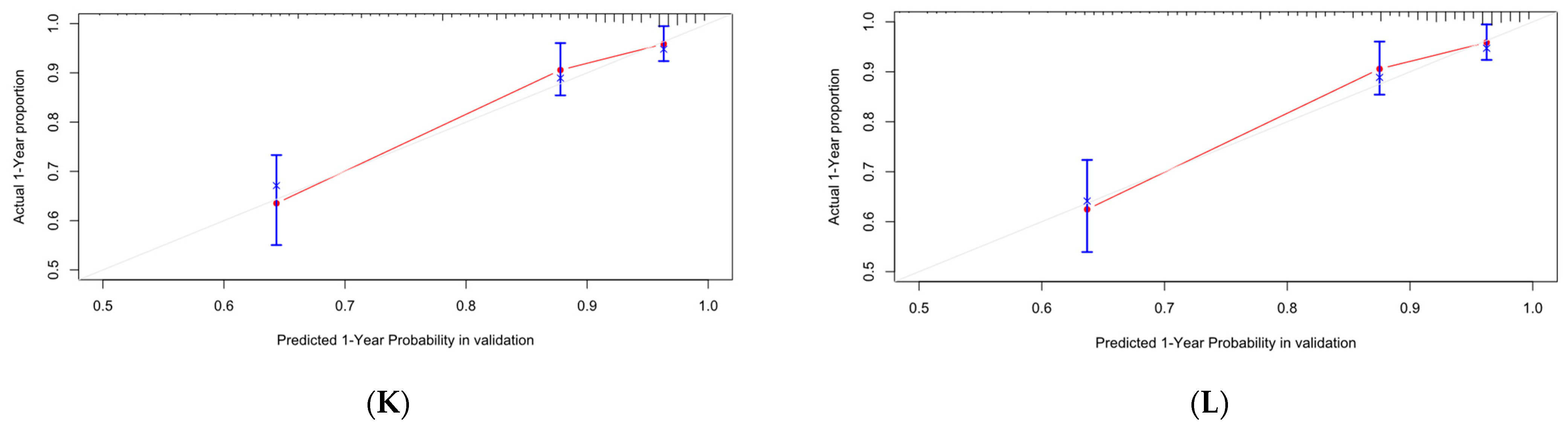
Figure 13.
Calibration curve of Cox-PH. (A–C) are 1-, 3-, and 5-year calibration curves for the OS training set; (D–F) are 1-, 3-, and 5-year calibration curves for the OS validation set; (G–I) are 1-, 3-, and 5-year calibration curves for the CSS training set; (J–L) are 1-, 3-, and 5-year calibration curves for the CSS validation set.
Figure 14.
ROC curve of Cox-PH. (A) is the ROC curve for the OS training set, (B) is the ROC curve for the OS validation set, (C) is the ROC curve for the CSS training set, and (D) is the ROC curve for the CSS validation set.
Figure 14.
ROC curve of Cox-PH. (A) is the ROC curve for the OS training set, (B) is the ROC curve for the OS validation set, (C) is the ROC curve for the CSS training set, and (D) is the ROC curve for the CSS validation set.
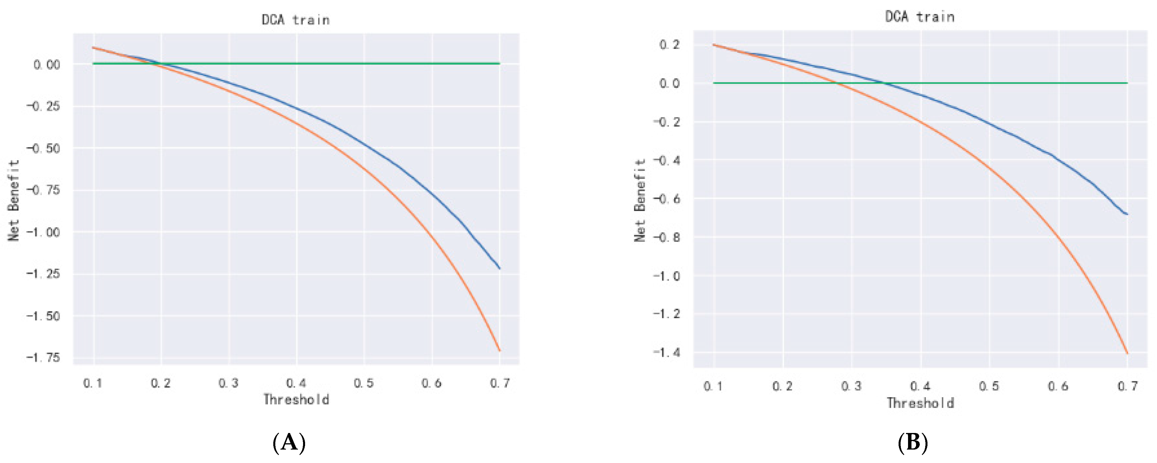
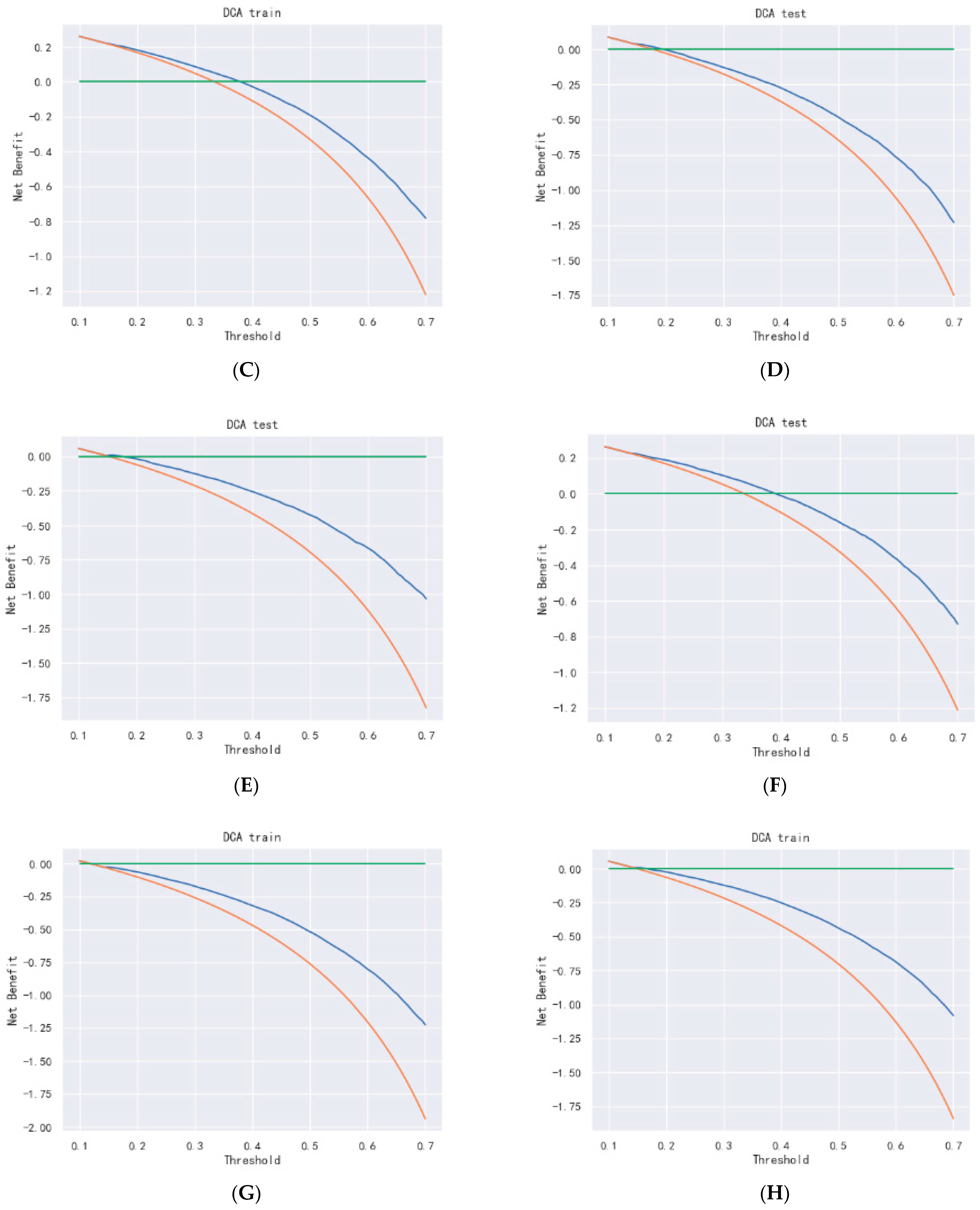
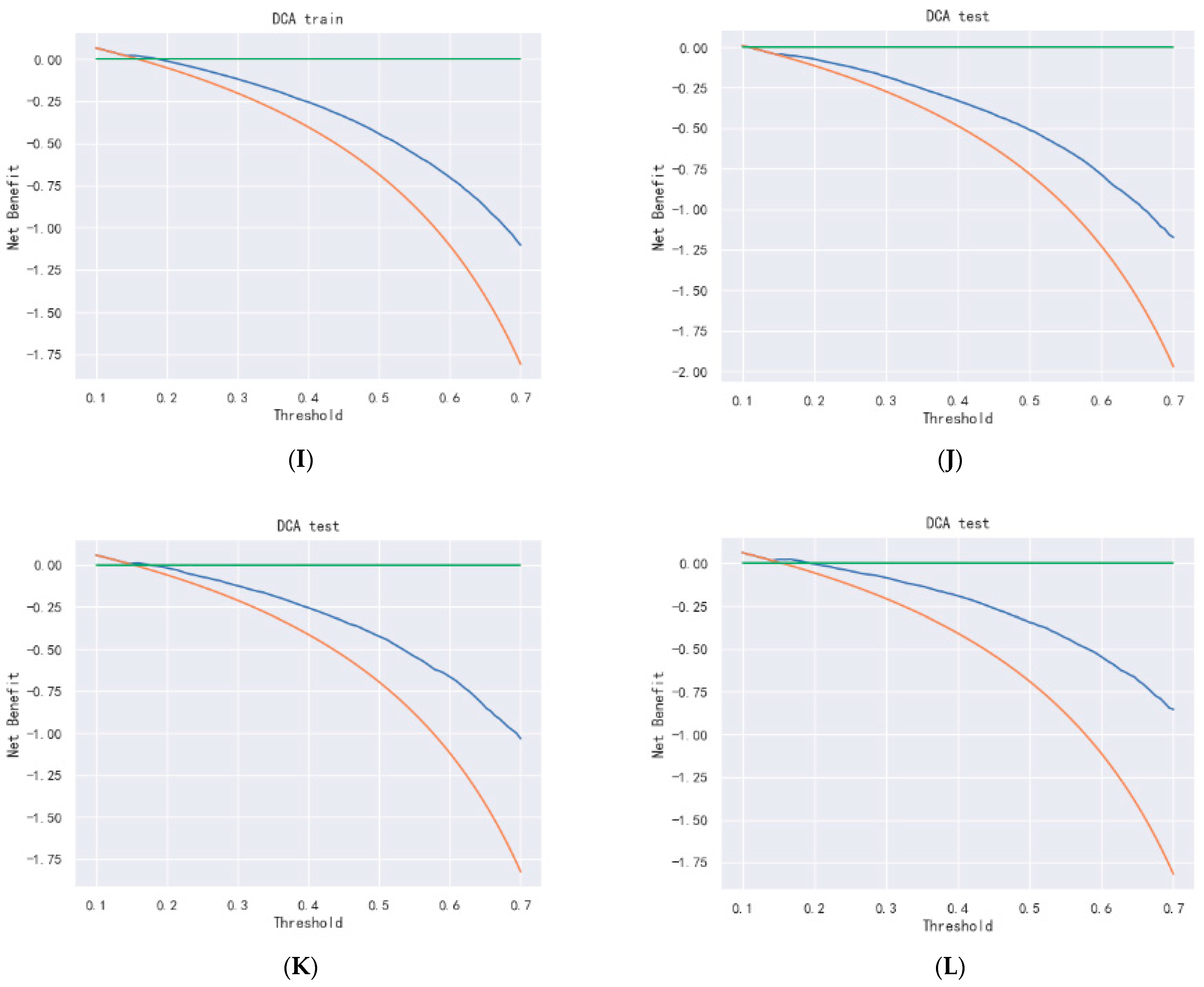
Figure 15.
DCA curve of Cox- PH. (A–C) are 1-, 3-, and 5-year DCA curves for OS training set; (D–F) are 1-, 3-, and 5-year DCA curves for OS validation set; (G–I) are 1-, 3-, and 5-year DCA curves for CSS training set; and (J–L) are 1-, 3-, and 5-year DCA curves for CSS validation set.
Figure 15.
DCA curve of Cox- PH. (A–C) are 1-, 3-, and 5-year DCA curves for OS training set; (D–F) are 1-, 3-, and 5-year DCA curves for OS validation set; (G–I) are 1-, 3-, and 5-year DCA curves for CSS training set; and (J–L) are 1-, 3-, and 5-year DCA curves for CSS validation set.
Figure 16.
Calibration curves of DeepSurv. (A–C) are 1-, 3-, and 5-year calibration curves for the OS training set. (D–F) are 1-, 3-, and 5-year calibration curves for the OS validation set; (G–I) are 1-, 3-, and 5-year calibration curves for the CSS training set; (J–L) are 1-, 3-, and 5-year calibration curves for the CSS validation set.
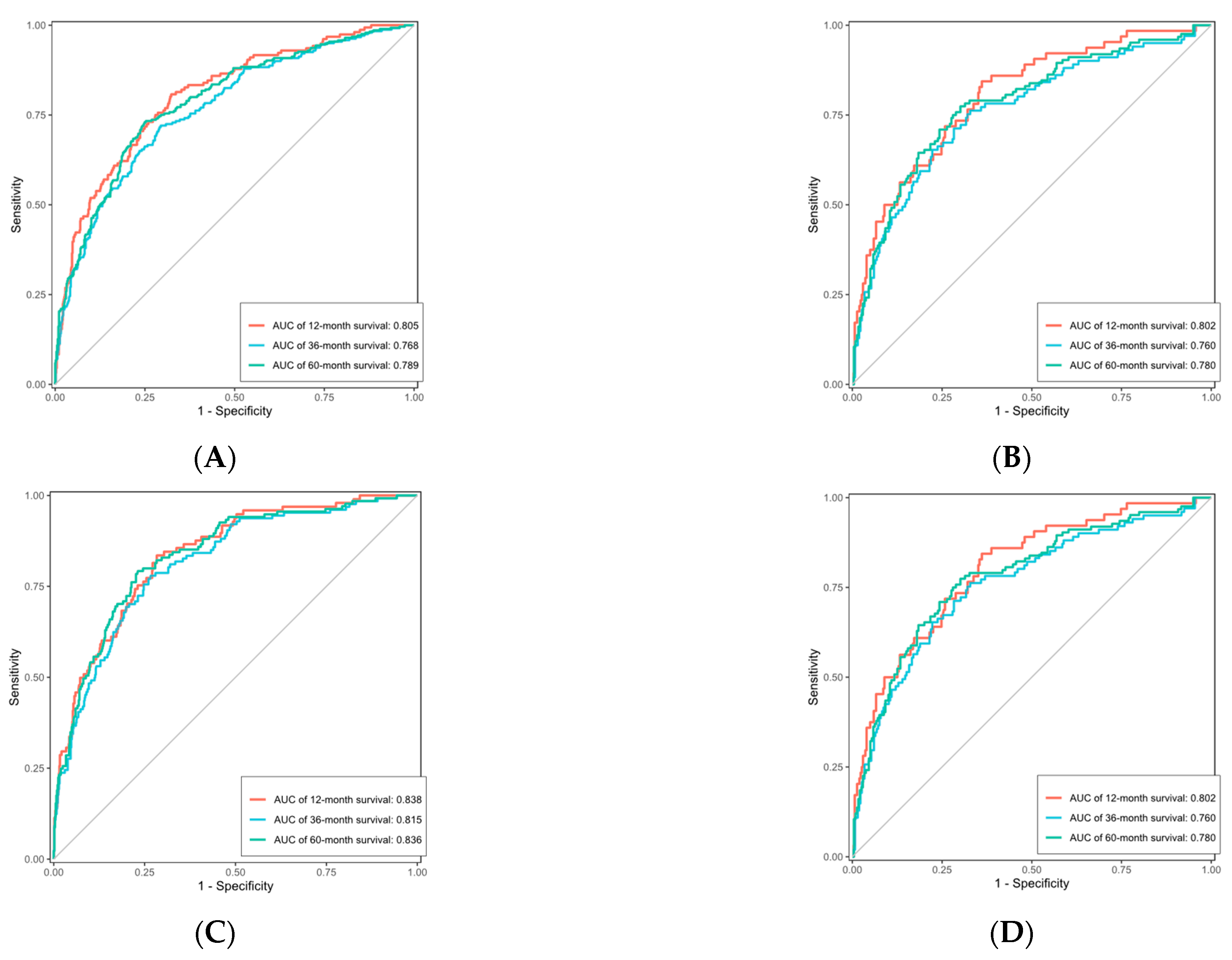
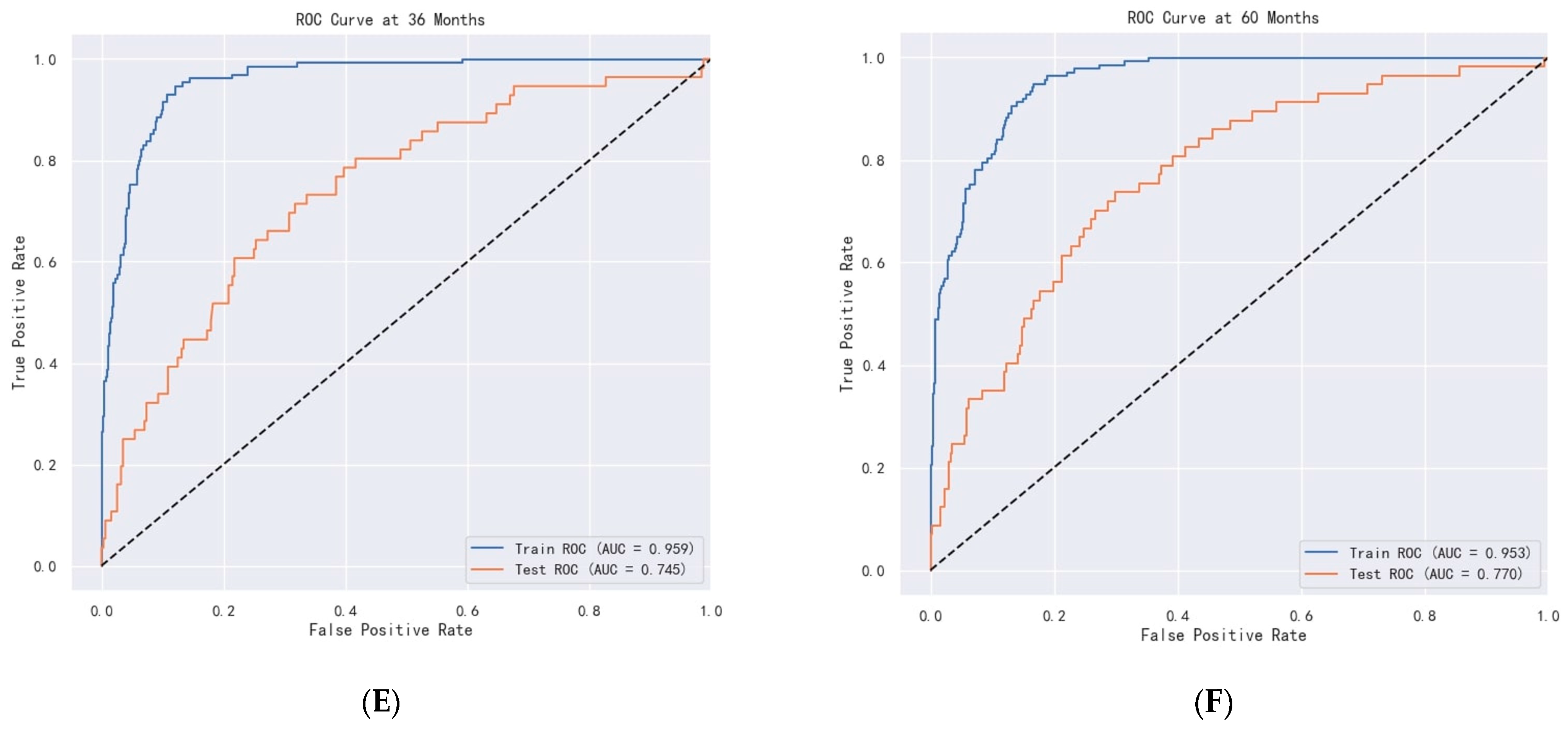
Figure 17.
ROC curve of DeepSurv. (A–C) are ROC curves for OS. (D–F) are ROC curves for CSS.
Figure 17.
ROC curve of DeepSurv. (A–C) are ROC curves for OS. (D–F) are ROC curves for CSS.
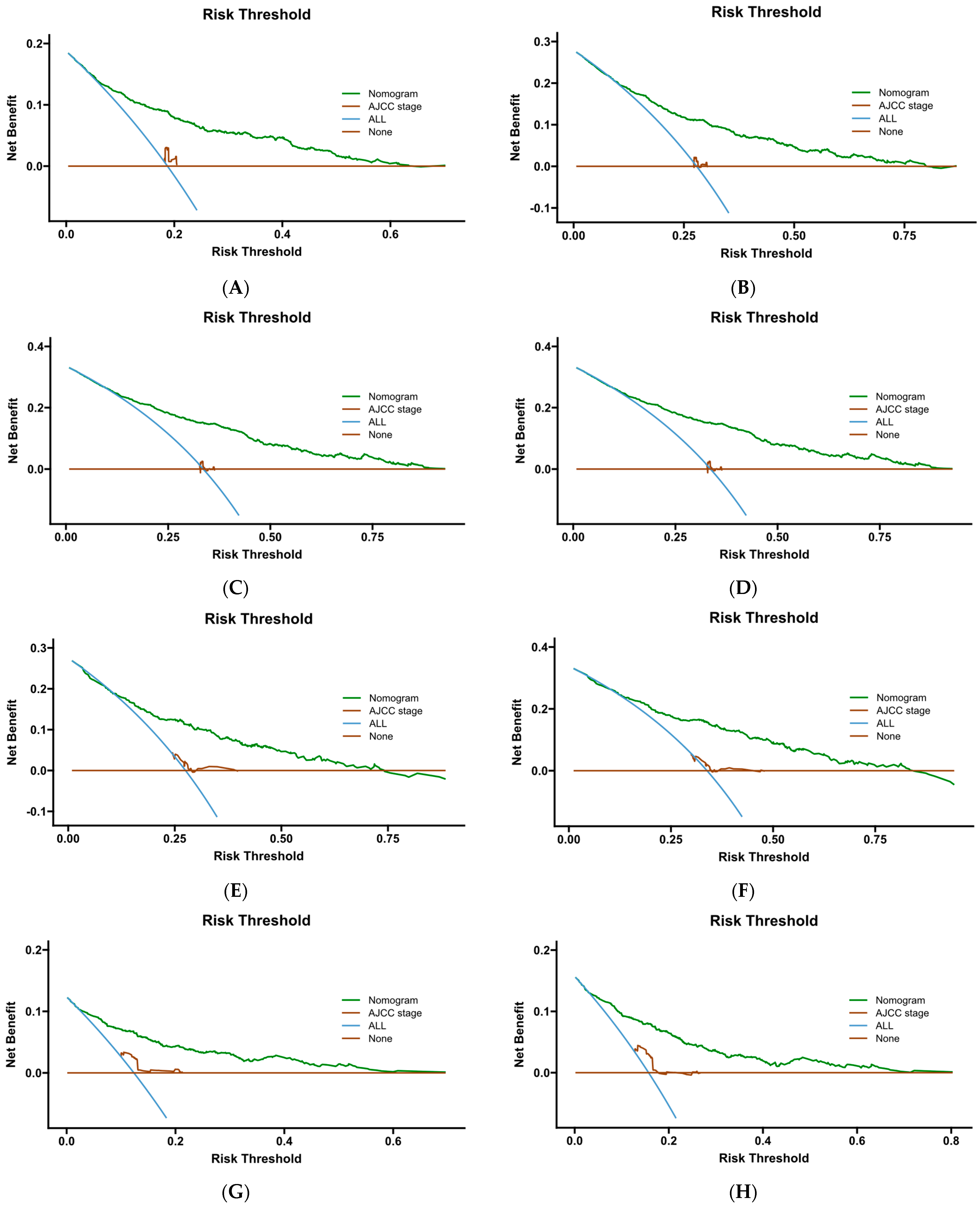
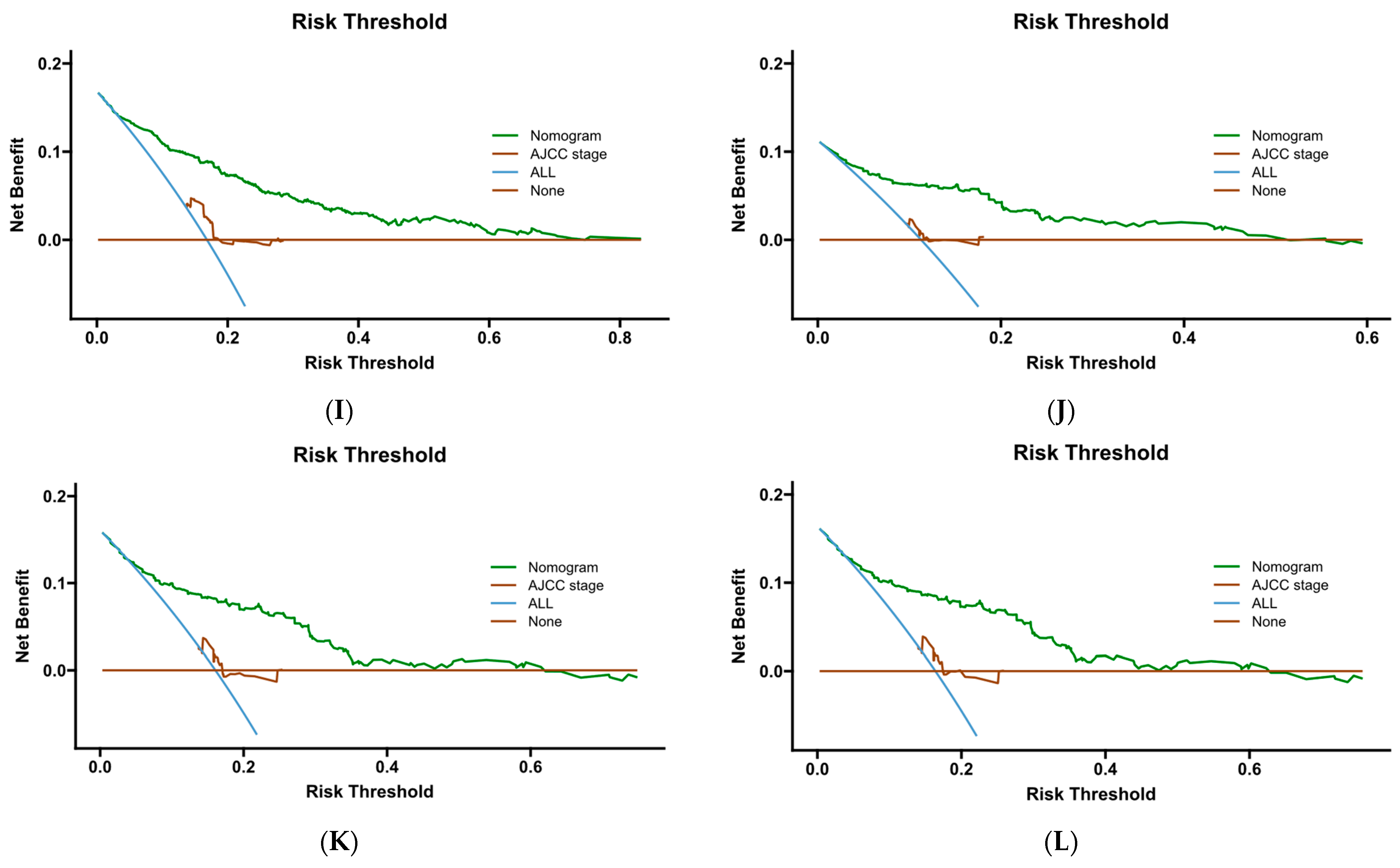
Figure 18.
DCA curve of DeepSurv. (A–C) are 1-, 3-, and 5-year DCA curves for OS training set; (D–F) are 1-, 3-, and 5-year DCA curves for OS validation set; (G–I) are 1-, 3-, and 5-year DCA curves for CSS training set; and (J–L) are 1-, 3-, and 5-year DCA curves for CSS validation set.
Figure 18.
DCA curve of DeepSurv. (A–C) are 1-, 3-, and 5-year DCA curves for OS training set; (D–F) are 1-, 3-, and 5-year DCA curves for OS validation set; (G–I) are 1-, 3-, and 5-year DCA curves for CSS training set; and (J–L) are 1-, 3-, and 5-year DCA curves for CSS validation set.
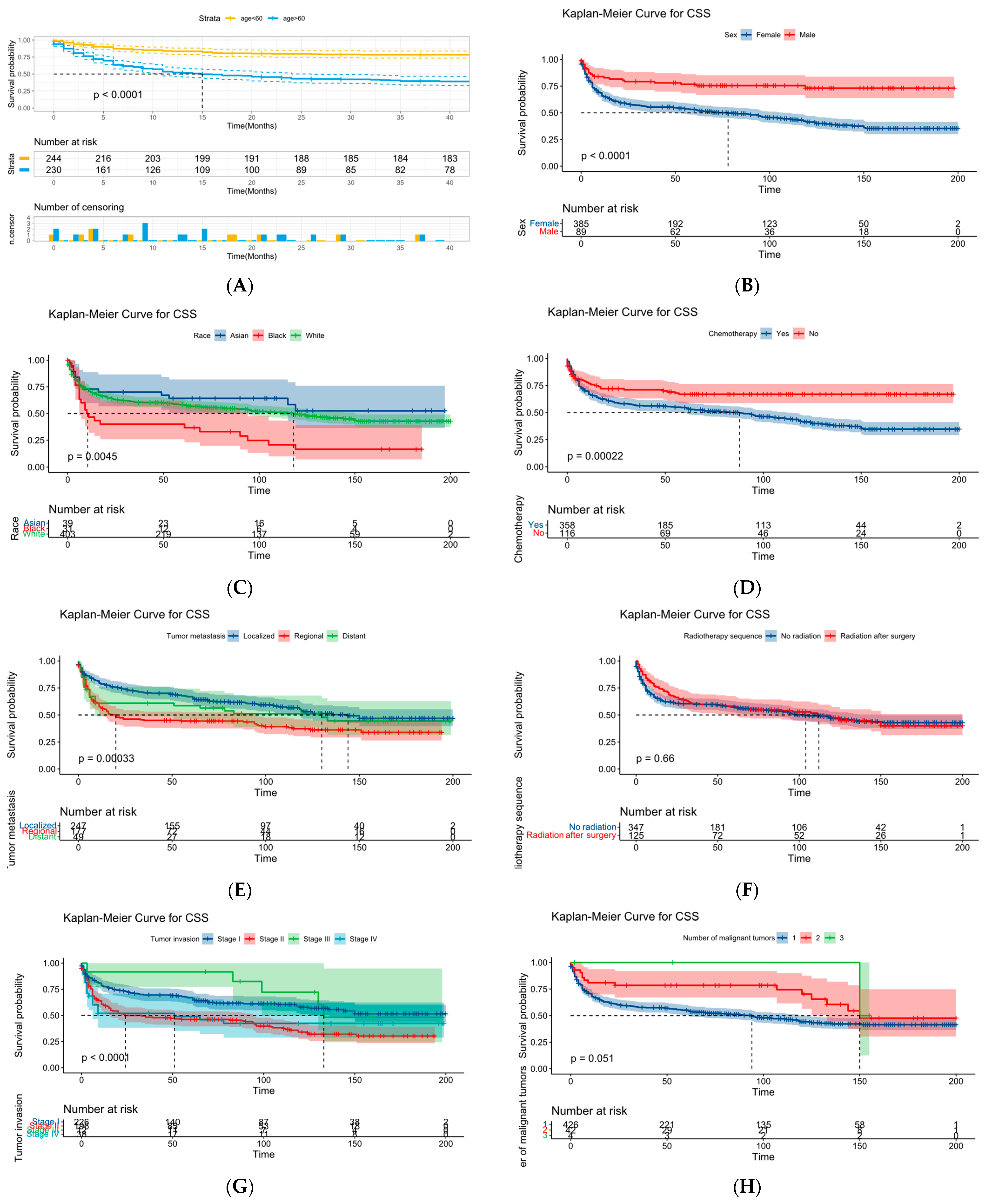
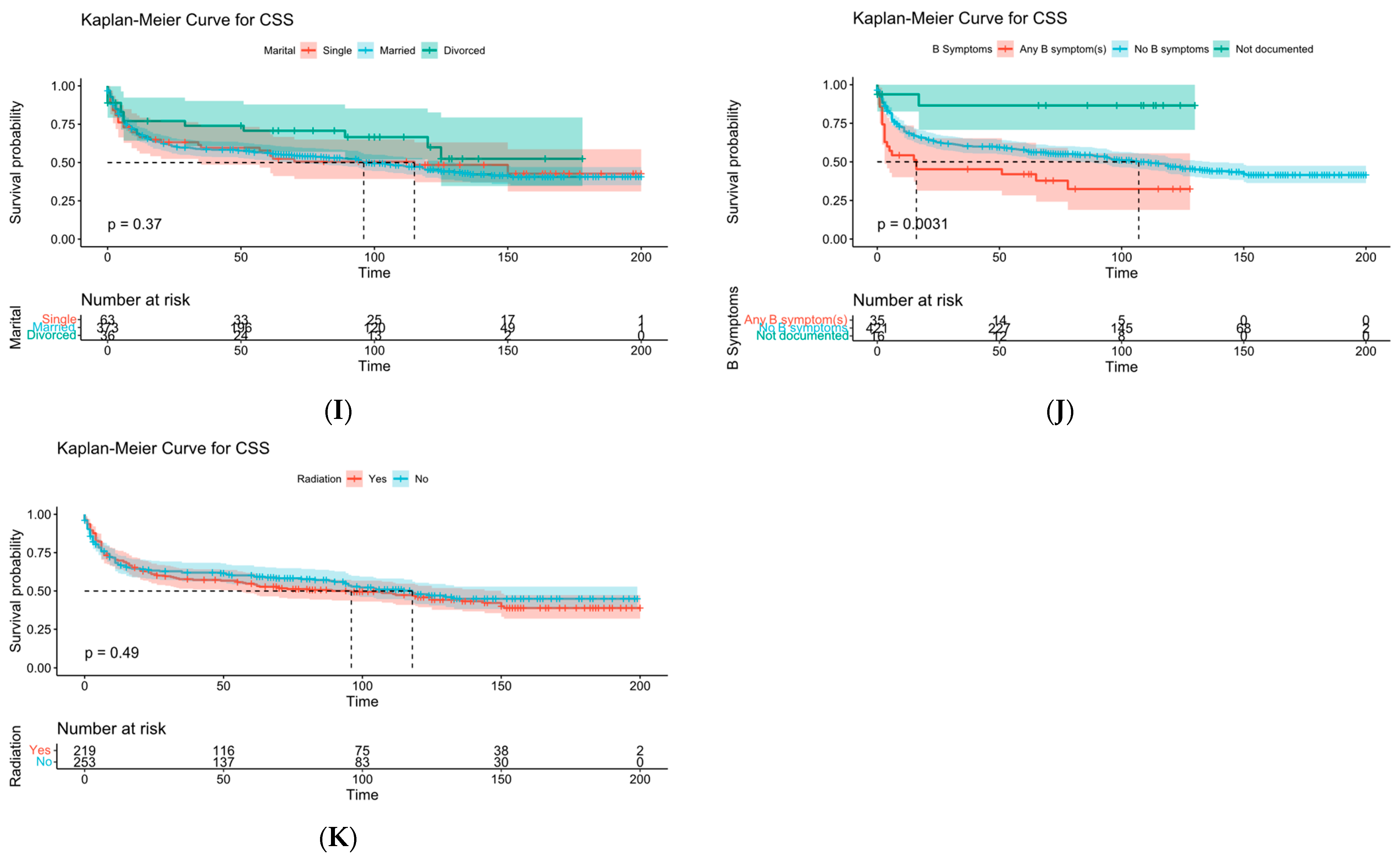
Figure 19.
KM survival curve analysis. (A) is age, (B) is sex, (C) is race, (D) is chemotherapy, (E) is distant metastasis, (F) is sequence of surgery and radiotherapy, (G) is degree of tumor invasion, (H) is number of malignancies, (I) is marital status, (J) is “B” symptom, and (K) is radiotherapy.
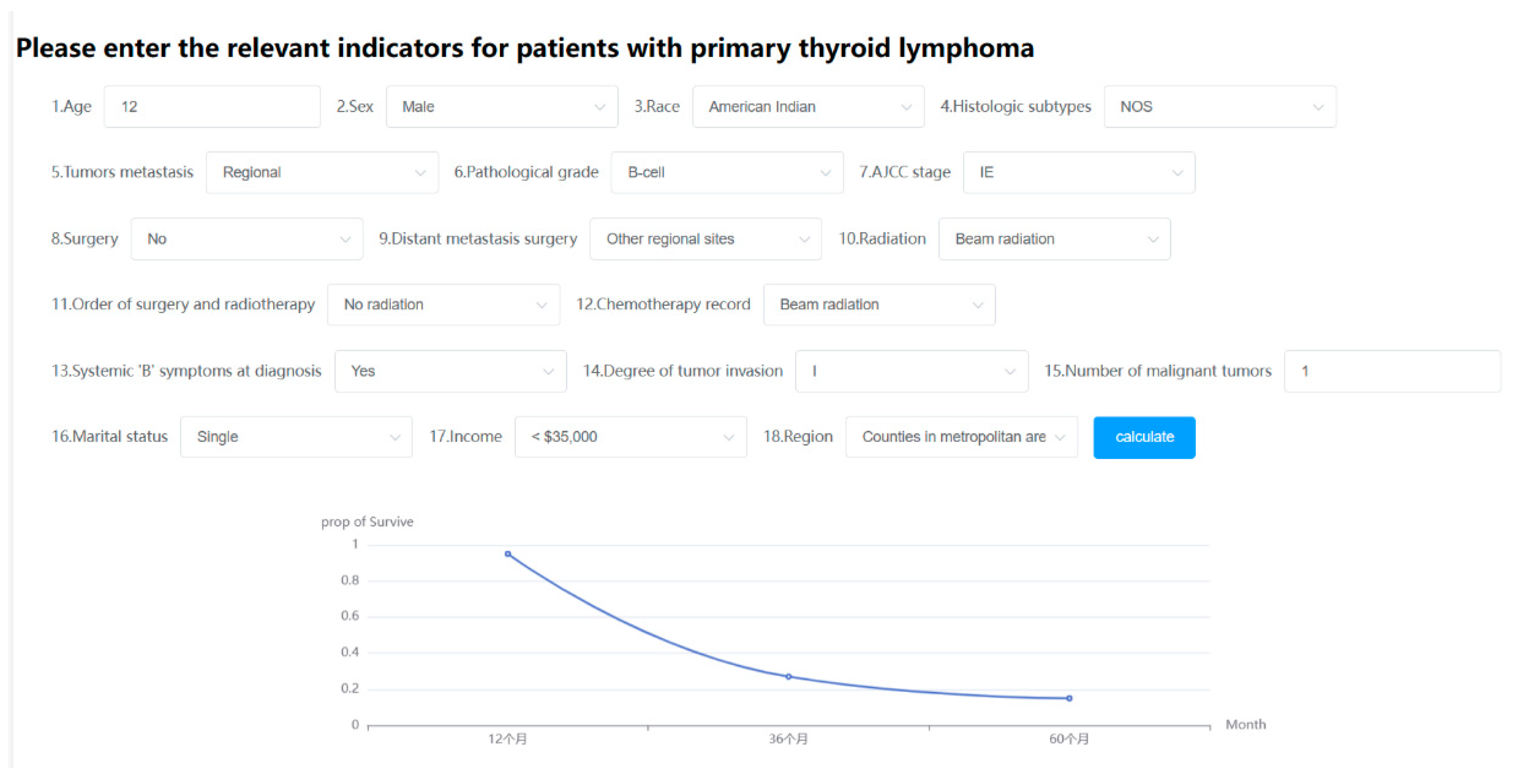
Figure 20.
Online web predictor.
Figure 20.
Online web predictor.
Table 1.
Patient clinical characteristics.
Table 1.
Patient clinical characteristics.
| Characteristics | Training Set | Validation Set | p-Value |
|---|
| Sex (%) | | | 0.703 |
| Female | 574 (68.99) | 238 (67.61) | |
| Male | 258 (31.01) | 114 (32.39) | |
| Race (%) | | | 0.967 |
| American Indian | 1 (0.12) | 3 (0.85) | |
| Asian | 69 (8.29) | 39 (11.08) | |
| Black | 24 (2.88) | 7 (1.99) | |
| White | 738 (88.70) | 303 (86.08) | |
| Histologic subtypes (%) | | | <0.001 |
| NOS | 89 (10.70) | 27 (7.67) | |
| Composite-site Hodgkin’s lymphoma | 3 (0.36) | 0 | |
| Small lymphocytic B cell | 6 (0.72) | 4 (1.14) | |
| Mantle cell lymphoma | 3 (0.36) | 3 (0.85) | |
| Mixed diffuse B cell | 2 (0.24) | 1 (0.28) | |
| DLBCL | 455 (54.69) | 190 (53.98) | |
| Burkitt’s lymphoma | 24 (2.88) | 13 (3.69) | |
| Follicular lymphoma | 68 (8.17) | 36 (10.23) | |
| Marginal zone lymphoma | 177 (21.27) | 76 (21.59) | |
| T-cell lymphoma | 5 (0.60) | 2 (0.57) | |
| Pathological grade (%) | | | 0.107 |
| B-cell | 823 (99.52) | 348 (98.86) | |
| Grade I | 3 (0.36) | 3 (0.85) | |
| Grade III | 1 (0.12) | 1 (0.28) | |
| T-cell | 5 (0.60) | 3 (0.85) | |
| Distant metastasis surgery (%) | | | 0.832 |
| Other regional sites | 828 (98.92) | 348 (98.86) | |
| Distant lymph node | 1 (0.12) | 2 (0.57) | |
| Distant site | 3 (0.36) | 2 (0.57) | |
| Radiation (%) | | | 0.146 |
| Beam radiation | 342 (41.11) | 144 (40.91) | |
| Method or source not specified | 16 (1.92) | 2 (0.57) | |
| Recommended | 5 (0.60) | 2 (0.57) | |
| Refused | 469 (56.37) | 204 (57.95) | |
| Order of surgery and radiotherapy (%) | | | 0.183 |
| No radiation | 643 (77.28) | 260 (73.86) | |
| Radiation prior to surgery | 188 (22.60) | 92 (26.14) | |
| Radiation after surgery | 1 (0.12) | 0 | |
| Chemotherapy record (%) | | | 0.526 |
| Yes | 525 (63.10) | 221 (62.78) | |
| No | 307 (36.90) | 131 (37.22) | |
| Systemic “B” symptoms at diagnosis (%) | | | 0.386 |
| Yes | 44 (5.29) | 13 (3.69) | |
| No | 726 (87.26) | 314 (89.20) | |
| Not documented | 62 (7.45) | 25 (7.10) | |
| Marital status (%) | | | 0.272 |
| Single | 100 (12.02) | 42 (11.93) | |
| Married | 657 (78.97) | 276 (78.41) | |
| Divorced | 75 (9.01) | 34 (9.66) | |
| Region(%) | | | 0.013 |
| Counties in metropolitan areas ge 1 million pop | 454 (54.57) | 182 (51.70) | |
| Counties in metropolitan areas of 250,000 to 1 million pop | 184 (22.12) | 67 (19.03) | |
| Counties in metropolitan areas of lt 250 thousand pop | 64 (7.69) | 34 (9.66) | |
| Nonmetropolitan counties adjacent to a metropolitan area | 67 (8.05) | 38 (10.80) | |
| Nonmetropolitan counties not adjacent to a metropolitan area | 63 (7.57) | 9 (2.56) | |
| Tumor metastasis (%) | | | 0.017 |
| Localized | 472 (56.73) | 190 (53.98) | |
| Regional | 265 (31.85) | 106 (30.11) | |
| Distant | 95 (11.42) | 46 (13.07) | |
| AJCC stage (%) | | | 0.151 |
| IE | 99 (11.90) | 45 (12.78) | |
| IEA | 321 (38.58) | 127 (36.08) | |
| IEB | 33 (3.97) | 14 (3.98) | |
| II | 1 (0.12) | 2 (0.57) | |
| IIE | 67 (8.05) | 24 (6.82) | |
| IIA | 10 (1.20) | 5 (1.42) | |
| IIEA | 173 (20.79) | 86 (24.43) | |
| IIEB | 33 (3.97) | 3 (0.85) | |
| IIIE | 1 (0.12) | 1 (0.28) | |
| IIIA | 3 (0.36) | 2 (0.57) | |
| IIIEA | 17 (2.04) | 7 (1.99) | |
| IIIEB | 2 (0.24) | 1 (0.28) | |
| IIIES | 0 | 1 (0.28) | |
| IIIESA | 2 (0.24) | 2 (0.57) | |
| IIIESB | 2 (0.24) | 0 | |
| IIISA | 1 (0.12) | 0 | |
| IV | 12 (1.44) | 3 (0.85) | |
| IVA | 34 (4.09) | 21 (5.97) | |
| IVB | 21 (2.52) | 8 (2.27) | |
| Surgery (%) | | | 0.003 |
| No | 376 (45.19) | 150 (42.61) | |
| Excision | 454 (54.57) | 202 (57.39) | |
| Unknown | 2 (0.24) | 0 | |
| Degree of tumor invasion (%) | | | 0.077 |
| I | 453 (54.45) | 186 (52.84) | |
| II | 284 (34.13) | 120 (34.09) | |
| III | 28 (3.37) | 14 (3.98) | |
| IV | 67 (8.05) | 32 (9.09) | |
| Number of malignant tumors (%) | | | 0.125 |
| 1 | 706 (84.86) | 301 (85.51) | |
| 2 | 107 (12.86) | 47 (13.35) | |
| 3 | 16 (1.92) | 4 (1.14) | |
| 4 | 3 (0.36) | 0 | |
| Income (%) | | | 0.692 |
| USD 35,000 | 14 (1.68) | 5 (1.42) | |
| USD 35,000–USD 39,999 | 19 (2.28) | 7 (1.99) | |
| USD 40,000–USD 44,999 | 34 (4.09) | 11 (3.13) | |
| USD 40,000–USD 44,999 | 35 (4.21) | 19 (5.40) | |
| USD 50,000–USD 54,999 | 59 (7.09) | 34 (9.66) | |
| USD 50,000–USD 54,999 | 69 (8.29) | 32 (9.09) | |
| USD 60,000–USD 64,999 | 77 (9.25) | 37 (10.51) | |
| USD 65,000–USD 69,999 | 148 (17.79) | 47 (13.35) | |
| USD 70,000–USD 74,999 | 77 (9.25) | 26 (7.39) | |
| USD 75,000+ | 300 (36.06) | 134 (38.07) | |
| Age | 64.819 ± 14.779 | 64.94 ± 14.564 | <0.001 |
Table 2.
Important features screened by different feature selection methods.
Table 2.
Important features screened by different feature selection methods.
| Feature Selection Methods | Screening Features |
|---|
| Univariate and Multivariate Cox Regression Analysis | Age, sex, histological type, tumor metastasis, radiotherapy, AJCC staging, surgery, sequence of surgery and radiotherapy, “B” symptoms, degree of tumor invasion, marital status, number of malignancies |
| Recursive Feature Elimination | Age, sex, histological type, radiotherapy, chemotherapy, “B” symptoms, marital status, region, tumor metastasis, AJCC stage, surgery, degree of tumor invasion, number of malignancies, income |
| Boruta Feature Selection | Age, histological type, tumor metastasis, AJCC staging, radiotherapy, chemotherapy, “B” symptoms, degree of tumor invasion, number of malignancies |
Table 3.
SMOTE oversampled modeling results.
Table 3.
SMOTE oversampled modeling results.
| | Accuracy | Recall | Precision | F1 |
|---|
| SVM | 0.532 | 0.532 | 0.544 | 0.486 |
| Logistic Regression | 0.691 | 0.691 | 0.693 | 0.691 |
| Random Forest | 0.755 | 0.755 | 0.766 | 0.754 |
| GBDT | 0.722 | 0.722 | 0.722 | 0.722 |
| XGBoost | 0.762 | 0.769 | 0.761 | 0.763 |
Table 4.
ClusterCentroids downsampling modeling results.
Table 4.
ClusterCentroids downsampling modeling results.
| | Accuracy | Recall | Precision | F1 |
|---|
| SVM | 0.593 | 0.593 | 0.596 | 0.590 |
| Logistic Regression | 0.701 | 0.702 | 0.701 | 0.706 |
| Random Forest | 0.703 | 0.713 | 0.707 | 0.715 |
| GBDT | 0.716 | 0.724 | 0.714 | 0.714 |
| XGBoost | 0.728 | 0.721 | 0.727 | 0.711 |
Table 5.
SMOTE Tomek link combinatorial sampling modeling results.
Table 5.
SMOTE Tomek link combinatorial sampling modeling results.
| | Accuracy | Recall | Precision | F1 |
|---|
| SVM | 0.563 | 0.563 | 0.598 | 0.529 |
| Logistic Regression | 0.675 | 0.675 | 0.678 | 0.675 |
| Random Forest | 0.801 | 0.801 | 0.801 | 0.801 |
| GBDT | 0.806 | 0.801 | 0.817 | 0.806 |
| XGBoost | 0.819 | 0.816 | 0.811 | 0.816 |
Table 6.
The c-index of the Cox-PH model.
Table 6.
The c-index of the Cox-PH model.
| | Train | Test |
|---|
| OS | 0.751 | 0.739 |
| CSS | 0.790 | 0.779 |
Table 7.
The c-index of the DeepSurv model.
Table 7.
The c-index of the DeepSurv model.
| | Train | Test |
|---|
| OS | 0.881 | 0.758 |
| CSS | 0.946 | 0.789 |


