


An Adaptive Non-Reference Approach for Characterizing and Assessing Image Quality in Multichannel GPR for Automatic Hyperbola Detection


Abstract
1. Introduction
Research Aim
2. Materials and Methods
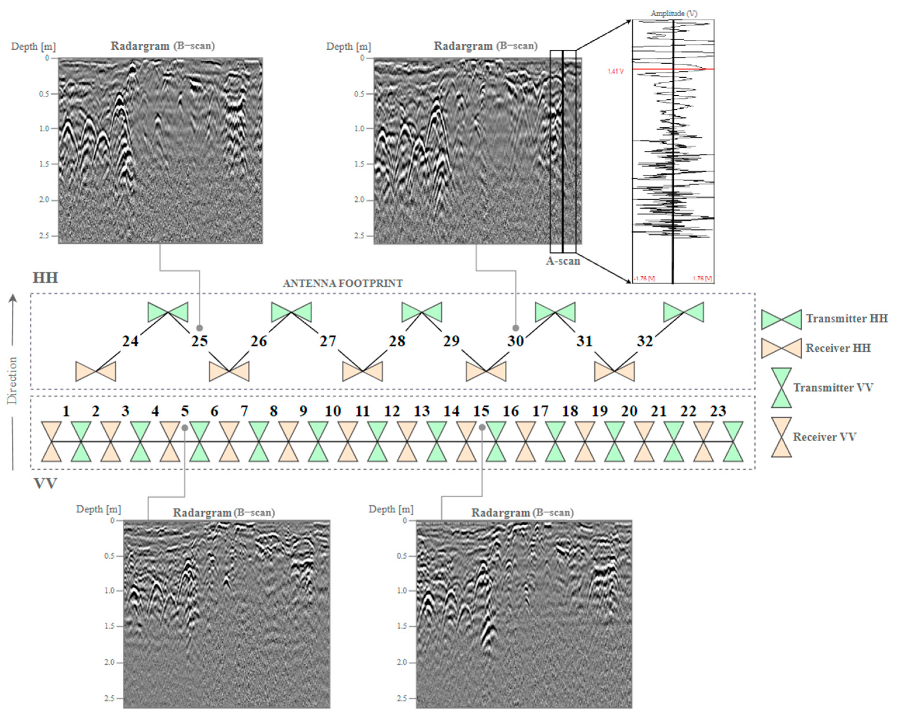
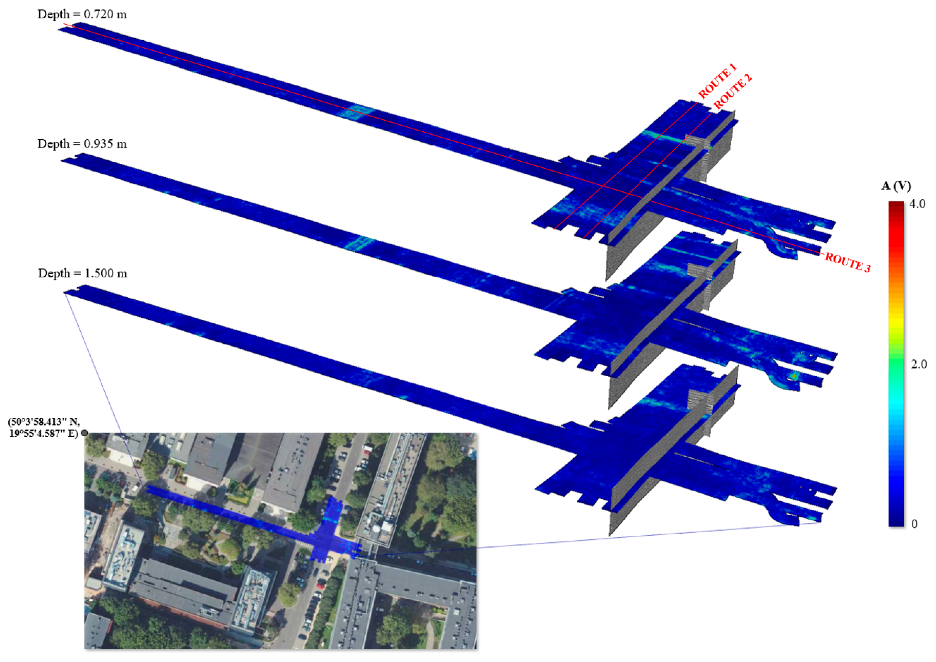
2.1. Study Area and Measurements
2.2. Processing of Images
- k—parameter defining the degree of noise in the image, k ϵ <0;1>;
- m—average standard deviation;
- s—local standard deviation in the neighborhood of the given pixel (x,y);
- R—range of the standard deviation.
2.3. Non-Reference Quality Assessment Metrics
2.3.1. Quality Metrics
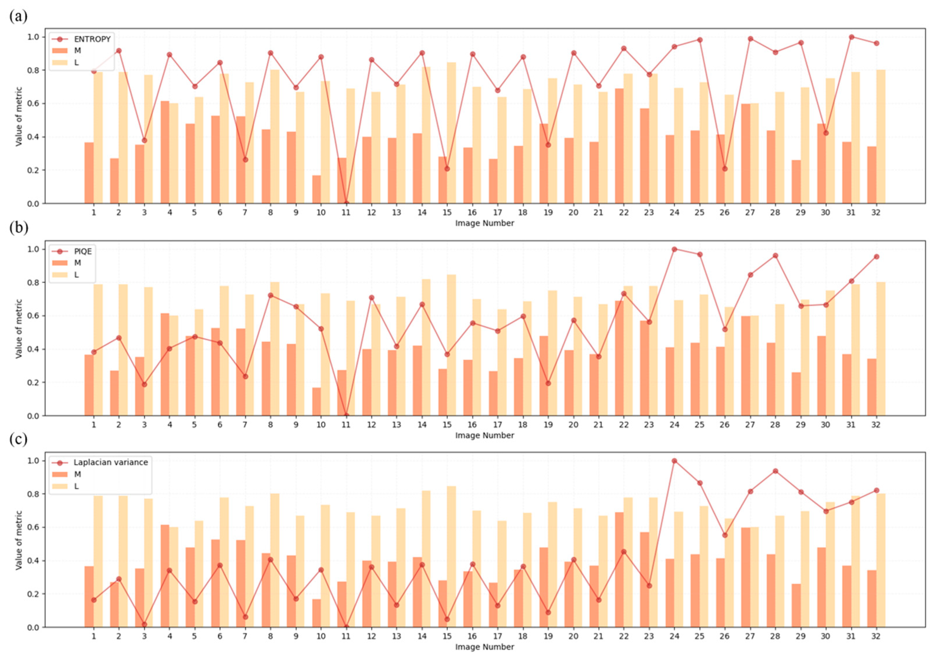
Entropy
- L—number of intensity values;
- pi—probability of occurrence of the given intensity i in the image.
PIQE (Perception-Based Image Quality Evaluator)
- —value of the pixel (x,y);
- —value of the local average within the pixel (x,y);
- —value of the local standard deviation within the pixel (x,y);
- C—value of the constant that prevents division by 0.
- —value of average intensity within the block;
- —number of pixels in the given block.
Laplacian Variance
- Li—Laplacian value in the ith pixel of the image;
- —average Laplacian value in the image;
- N—number of pixels in the image.
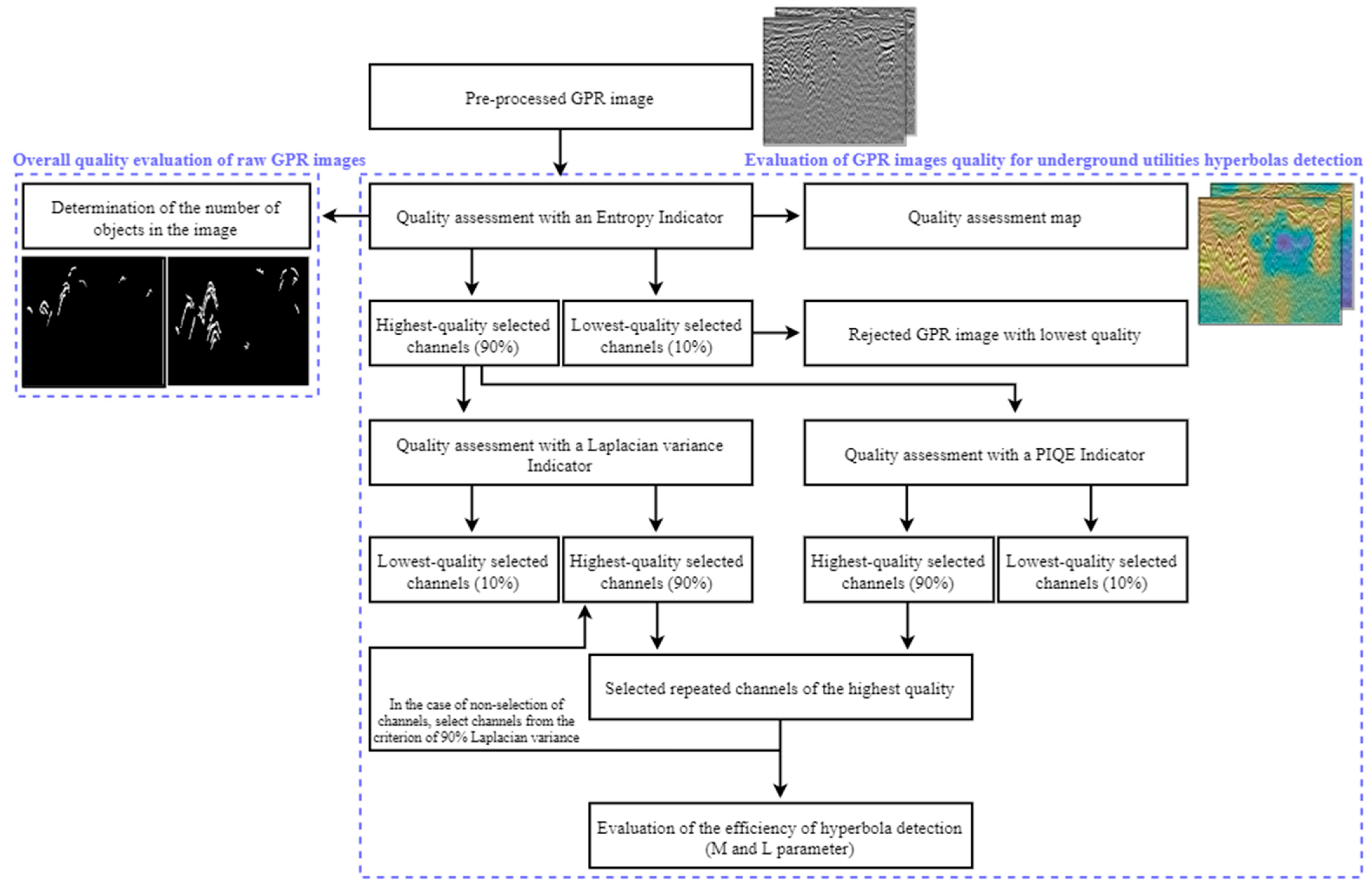
2.4. Adaptive Method of Radargram Quality Assessment
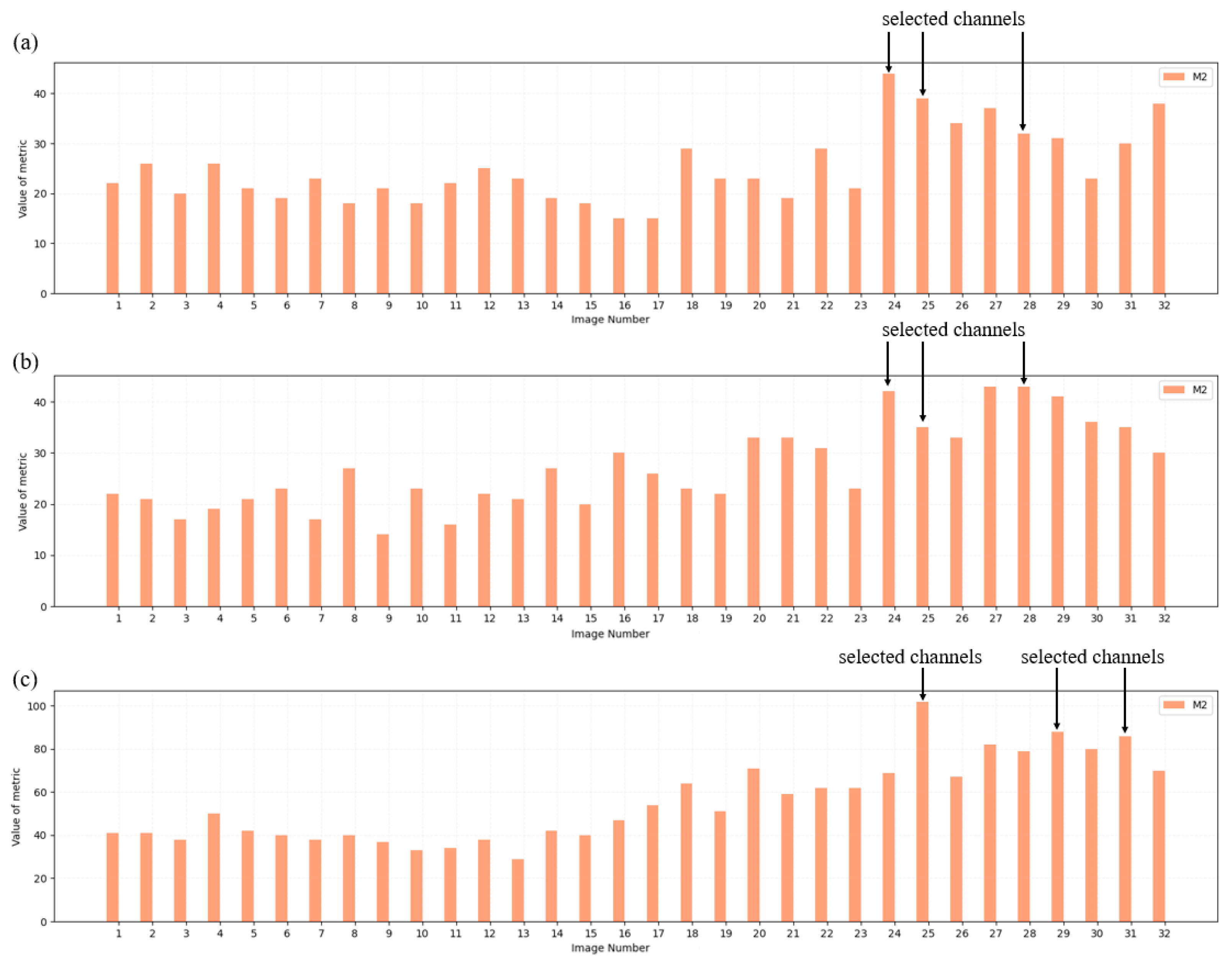
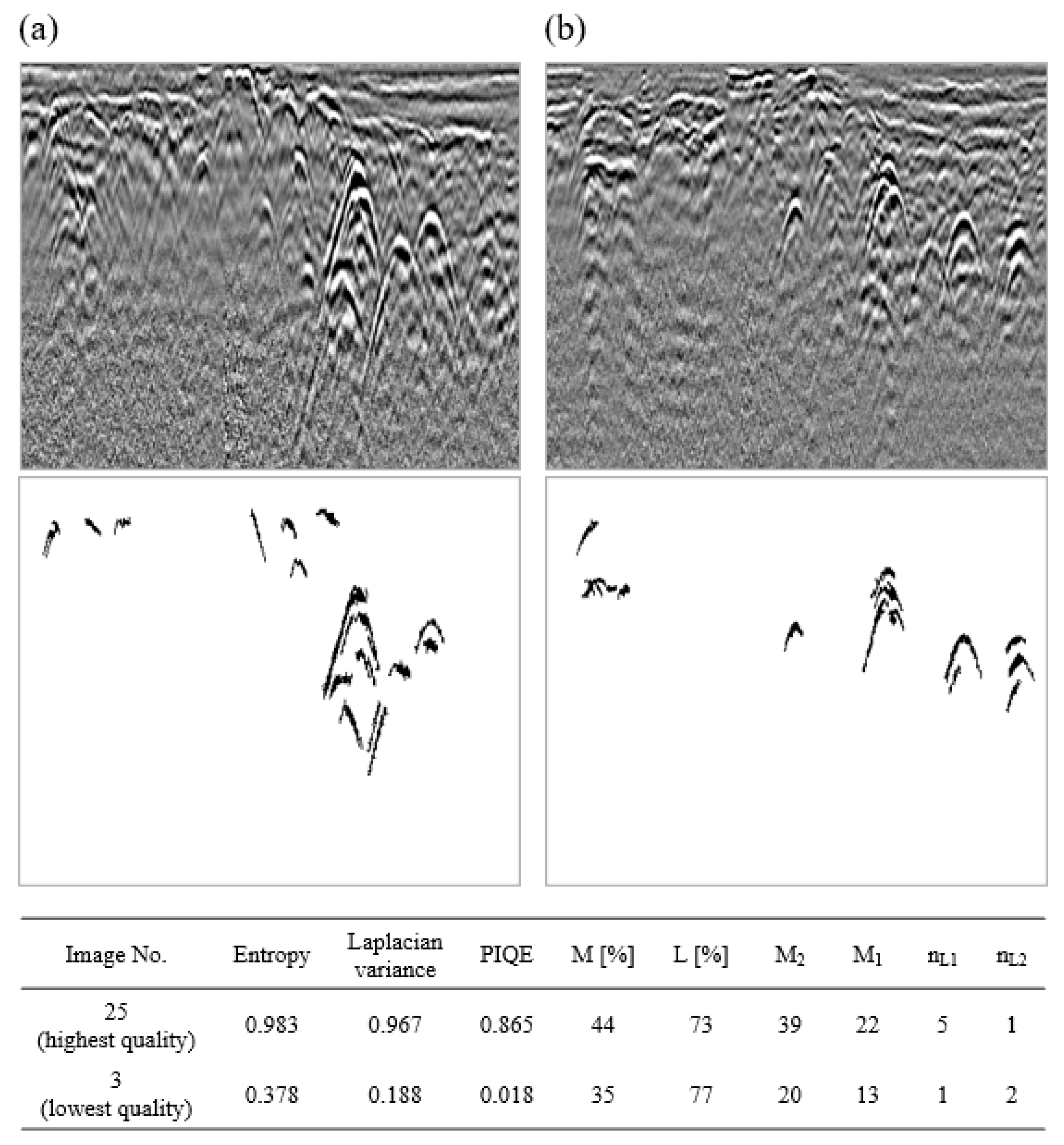
- M1—the number of objects detected in the target image (i.e., after the pre-processing stage, filtration, and the application of conditions CS, CC, and CD)—Step 4 in Figure 3;
- M2—the number of objects detected in the output image (i.e., after pre-processing)—Step 1 in Figure 3.
- NL—number of all objects detected in the image (the number is determined automatically);
- nL1—number of detected objects not being underground utility networks (the number is calculated manually);
- nL2—number of undetected objects being underground utility networks (the number is calculated manually).
3. Results and Discussion
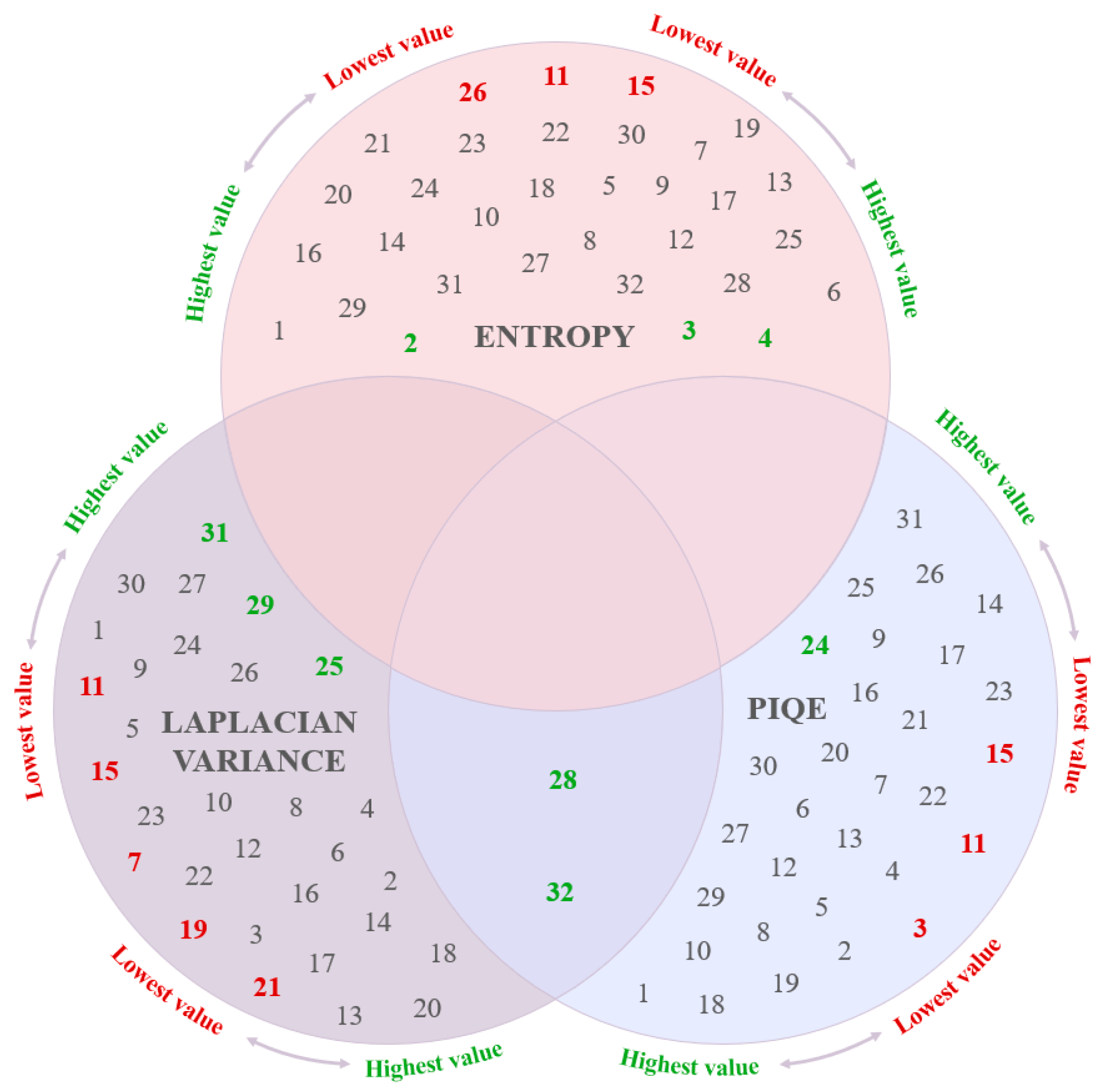
3.1. Image Quality Assessment
3.1.1. Overall Quality Assessment of Raw GPR Images
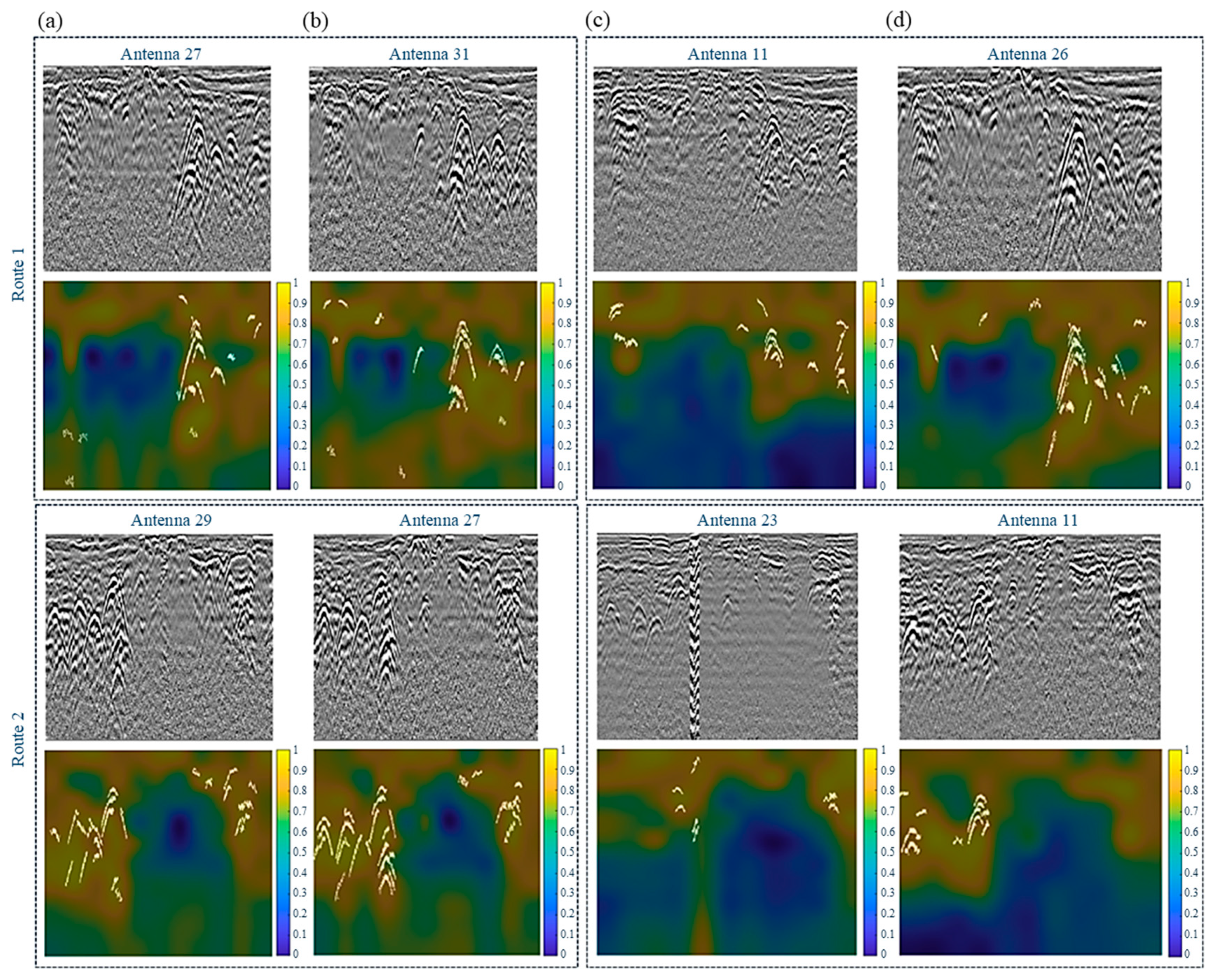
3.1.2. Assessment of the Quality of GPR Images for the Detection of Hyperbolas Representing Underground Utilities
- The operating principle of the PIQE algorithm consists in dividing the image into smaller regions, where the level of noise and artifacts is analyzed locally. Areas characterized by large artifacts are identified as low-quality areas. The PIQE algorithm consists in dividing the image into blocks (e.g., of the size of 8 × 8, 16 × 16, 32 × 32). The value of the PIQE index is calculated based on the number of degraded blocks and all blocks within the image. Dividing the image into smaller blocks gives a better assessment of quality than the NIQE or BRISQUE index [58,59].
- The BRISQUE indicator compares the image with a default model generated from images of natural scenes with similar distortions. Radargrams do not represent natural scenes. Therefore, the BRISQUE indicator, based on the statistics of natural images, will not reliably assess the quality of GPR-acquired images.
3.2. Verification of Detection Efficiency
4. Conclusions
Author Contributions
Funding
Institutional Review Board Statement
Informed Consent Statement
Data Availability Statement
Conflicts of Interest
Appendix A


| Route No. | Image No. | Entropy | Laplacian Variance | PIQE | NIQE | BRISQUE | M | L |
|---|---|---|---|---|---|---|---|---|
| 3 | 1 | 0.903 | 0.281 | 0.424 | 0.814 | 0.505 | 0.659 | 0.818 |
| 3 | 2 | 1.000 | 0.369 | 0.260 | 0.438 | 0.173 | 0.634 | 0.750 |
| 3 | 3 | 0.907 | 0.134 | 0.000 | 0.513 | 0.000 | 0.605 | 0.636 |
| 3 | 4 | 0.976 | 0.445 | 0.273 | 0.672 | 0.438 | 0.600 | 0.750 |
| 3 | 5 | 0.598 | 0.145 | 0.304 | 0.608 | 0.766 | 0.690 | 0.636 |
| 3 | 6 | 0.822 | 0.420 | 0.473 | 0.673 | 0.985 | 0.575 | 0.750 |
| 3 | 7 | 0.291 | 0.073 | 0.348 | 0.473 | 0.819 | 0.605 | 0.714 |
| 3 | 8 | 0.757 | 0.424 | 0.459 | 0.442 | 0.692 | 0.700 | 0.692 |
| 3 | 9 | 0.592 | 0.172 | 0.550 | 0.404 | 0.601 | 0.514 | 0.727 |
| 3 | 10 | 0.753 | 0.363 | 0.440 | 0.850 | 0.919 | 0.606 | 0.650 |
| 3 | 11 | 0.000 | 0.000 | 0.062 | 0.466 | 0.848 | 0.676 | 0.636 |
| 3 | 12 | 0.771 | 0.362 | 0.460 | 0.624 | 1.000 | 0.526 | 0.750 |
| 3 | 13 | 0.528 | 0.108 | 0.340 | 0.521 | 0.450 | 0.690 | 0.636 |
| 3 | 14 | 0.710 | 0.322 | 0.373 | 0.795 | 0.798 | 0.619 | 0.818 |
| 3 | 15 | 0.084 | 0.014 | 0.207 | 0.731 | 0.999 | 0.525 | 0.750 |
| 3 | 16 | 0.679 | 0.351 | 0.505 | 0.808 | 0.908 | 0.745 | 0.636 |
| 3 | 17 | 0.535 | 0.128 | 0.372 | 0.679 | 0.830 | 0.630 | 0.750 |
| 3 | 18 | 0.647 | 0.310 | 0.418 | 0.801 | 0.788 | 0.672 | 0.714 |
| 3 | 19 | 0.216 | 0.077 | 0.246 | 0.807 | 0.823 | 0.725 | 0.692 |
| 3 | 20 | 0.662 | 0.282 | 0.492 | 1.000 | 0.913 | 0.662 | 0.727 |
| 3 | 21 | 0.487 | 0.083 | 0.350 | 0.910 | 0.620 | 0.576 | 0.650 |
| 3 | 22 | 0.486 | 0.143 | 0.296 | 0.387 | 0.651 | 0.597 | 0.600 |
| 3 | 23 | 0.486 | 0.143 | 0.296 | 0.387 | 0.651 | 0.597 | 0.636 |
| 3 | 24 | 0.652 | 0.767 | 1.000 | 0.408 | 0.732 | 0.507 | 0.636 |
| 3 | 25 | 0.798 | 0.901 | 0.853 | 0.476 | 0.848 | 0.637 | 0.750 |
| 3 | 26 | 0.122 | 0.629 | 0.656 | 0.312 | 0.883 | 0.537 | 0.636 |
| 3 | 27 | 0.869 | 0.875 | 0.823 | 0.306 | 0.901 | 0.646 | 0.750 |
| 3 | 28 | 0.830 | 0.973 | 0.963 | 0.000 | 0.761 | 0.620 | 0.800 |
| 3 | 29 | 0.894 | 1.000 | 0.810 | 0.146 | 0.898 | 0.534 | 0.773 |
| 3 | 30 | 0.394 | 0.853 | 0.825 | 0.051 | 0.987 | 0.513 | 0.850 |
| 3 | 31 | 0.871 | 0.988 | 0.847 | 0.386 | 0.889 | 0.628 | 0.810 |
| 3 | 32 | 0.852 | 0.951 | 0.863 | 0.039 | 0.529 | 0.700 | 0.733 |
| 1 | 1 | 0.795 | 0.162 | 0.382 | 0.927 | 0.846 | 0.364 | 0.786 |
| 1 | 2 | 0.918 | 0.289 | 0.468 | 0.493 | 0.527 | 0.269 | 0.789 |
| 1 | 3 | 0.378 | 0.018 | 0.188 | 0.299 | 0.927 | 0.350 | 0.769 |
| 1 | 4 | 0.893 | 0.341 | 0.403 | 0.527 | 0.527 | 0.615 | 0.600 |
| 1 | 5 | 0.703 | 0.153 | 0.474 | 0.639 | 0.680 | 0.476 | 0.636 |
| 1 | 6 | 0.846 | 0.373 | 0.436 | 0.397 | 0.601 | 0.526 | 0.778 |
| 1 | 7 | 0.264 | 0.063 | 0.235 | 0.797 | 0.990 | 0.522 | 0.727 |
| 1 | 8 | 0.905 | 0.406 | 0.722 | 0.515 | 0.626 | 0.444 | 0.800 |
| 1 | 9 | 0.696 | 0.169 | 0.654 | 0.545 | 0.518 | 0.429 | 0.667 |
| 1 | 10 | 0.878 | 0.346 | 0.521 | 0.990 | 0.892 | 0.167 | 0.733 |
| 1 | 11 | 0.000 | 0.000 | 0.000 | 0.544 | 0.807 | 0.273 | 0.688 |
| 1 | 12 | 0.862 | 0.361 | 0.710 | 0.538 | 0.313 | 0.400 | 0.667 |
| 1 | 13 | 0.715 | 0.132 | 0.416 | 0.549 | 0.549 | 0.391 | 0.714 |
| 1 | 14 | 0.905 | 0.375 | 0.667 | 0.735 | 0.732 | 0.421 | 0.818 |
| 1 | 15 | 0.209 | 0.048 | 0.368 | 1.000 | 1.000 | 0.278 | 0.846 |
| 1 | 16 | 0.896 | 0.379 | 0.556 | 0.709 | 0.927 | 0.333 | 0.700 |
| 1 | 17 | 0.678 | 0.130 | 0.508 | 0.473 | 0.333 | 0.267 | 0.636 |
| 1 | 18 | 0.878 | 0.366 | 0.595 | 0.569 | 0.490 | 0.345 | 0.684 |
| 1 | 19 | 0.352 | 0.089 | 0.194 | 0.358 | 0.891 | 0.478 | 0.750 |
| 1 | 20 | 0.905 | 0.404 | 0.572 | 0.511 | 0.658 | 0.391 | 0.714 |
| 1 | 21 | 0.706 | 0.164 | 0.353 | 0.234 | 0.296 | 0.368 | 0.667 |
| 1 | 22 | 0.930 | 0.454 | 0.733 | 0.410 | 0.502 | 0.690 | 0.778 |
| 1 | 23 | 0.773 | 0.250 | 0.563 | 0.747 | 0.634 | 0.571 | 0.778 |
| 1 | 24 | 0.940 | 1.000 | 1.000 | 0.131 | 0.463 | 0.409 | 0.692 |
| 1 | 25 | 0.983 | 0.865 | 0.967 | 0.161 | 0.126 | 0.436 | 0.727 |
| 1 | 26 | 0.207 | 0.552 | 0.519 | 0.363 | 0.857 | 0.412 | 0.650 |
| 1 | 27 | 0.990 | 0.815 | 0.844 | 0.248 | 0.154 | 0.595 | 0.600 |
| 1 | 28 | 0.907 | 0.937 | 0.960 | 0.000 | 0.250 | 0.438 | 0.667 |
| 1 | 29 | 0.965 | 0.813 | 0.658 | 0.335 | 0.159 | 0.258 | 0.696 |
| 1 | 30 | 0.423 | 0.696 | 0.666 | 0.461 | 0.952 | 0.478 | 0.750 |
| 1 | 31 | 1.000 | 0.750 | 0.807 | 0.255 | 0.426 | 0.367 | 0.789 |
| 1 | 32 | 0.960 | 0.820 | 0.956 | 0.105 | 0.000 | 0.342 | 0.800 |
| 2 | 1 | 0.666 | 0.354 | 0.503 | 0.270 | 0.650 | 0.500 | 0.818 |
| 2 | 2 | 0.824 | 0.465 | 0.650 | 0.381 | 0.458 | 0.429 | 0.750 |
| 2 | 3 | 0.307 | 0.152 | 0.407 | 0.598 | 0.667 | 0.353 | 0.636 |
| 2 | 4 | 0.785 | 0.528 | 0.567 | 0.524 | 0.488 | 0.526 | 0.556 |
| 2 | 5 | 0.576 | 0.324 | 0.611 | 0.513 | 0.548 | 0.381 | 0.769 |
| 2 | 6 | 0.746 | 0.532 | 0.740 | 0.621 | 0.638 | 0.391 | 0.714 |
| 2 | 7 | 0.277 | 0.200 | 0.407 | 0.575 | 0.760 | 0.294 | 0.750 |
| 2 | 8 | 0.779 | 0.563 | 0.722 | 0.446 | 0.574 | 0.519 | 0.769 |
| 2 | 9 | 0.600 | 0.322 | 0.600 | 0.579 | 0.468 | 0.357 | 0.667 |
| 2 | 10 | 0.784 | 0.541 | 0.706 | 0.993 | 0.794 | 0.478 | 0.833 |
| 2 | 11 | 0.011 | 0.156 | 0.300 | 0.544 | 0.968 | 0.375 | 0.800 |
| 2 | 12 | 0.793 | 0.593 | 0.961 | 1.000 | 0.715 | 0.364 | 0.786 |
| 2 | 13 | 0.623 | 0.341 | 0.705 | 0.586 | 0.591 | 0.381 | 0.786 |
| 2 | 14 | 0.769 | 0.509 | 0.768 | 0.941 | 0.786 | 0.481 | 0.750 |
| 2 | 15 | 0.176 | 0.160 | 0.442 | 0.608 | 0.776 | 0.300 | 0.714 |
| 2 | 16 | 0.709 | 0.521 | 0.817 | 0.660 | 0.795 | 0.400 | 0.833 |
| 2 | 17 | 0.544 | 0.270 | 0.673 | 0.716 | 0.616 | 0.385 | 0.688 |
| 2 | 18 | 0.724 | 0.487 | 0.782 | 0.580 | 0.555 | 0.261 | 0.765 |
| 2 | 19 | 0.318 | 0.193 | 0.480 | 0.634 | 0.917 | 0.364 | 0.643 |
| 2 | 20 | 0.758 | 0.440 | 0.601 | 0.552 | 0.718 | 0.333 | 0.682 |
| 2 | 21 | 0.590 | 0.188 | 0.537 | 0.404 | 0.382 | 0.455 | 0.667 |
| 2 | 22 | 0.535 | 0.228 | 0.514 | 0.271 | 0.186 | 0.323 | 0.714 |
| 2 | 23 | 0.000 | 0.000 | 0.000 | 0.000 | 0.000 | 0.696 | 0.429 |
| 2 | 24 | 0.918 | 0.961 | 0.921 | 0.278 | 0.701 | 0.500 | 0.833 |
| 2 | 25 | 0.966 | 0.973 | 0.652 | 0.274 | 0.626 | 0.429 | 0.750 |
| 2 | 26 | 0.217 | 0.617 | 0.568 | 0.242 | 1.000 | 0.424 | 0.789 |
| 2 | 27 | 0.994 | 0.913 | 1.000 | 0.469 | 0.704 | 0.349 | 0.750 |
| 2 | 28 | 0.965 | 1.000 | 0.938 | 0.360 | 0.546 | 0.302 | 0.800 |
| 2 | 29 | 1.000 | 0.939 | 0.983 | 0.336 | 0.267 | 0.463 | 0.773 |
| 2 | 30 | 0.520 | 0.783 | 0.605 | 0.342 | 0.696 | 0.444 | 0.850 |
| 2 | 31 | 0.968 | 0.875 | 0.675 | 0.468 | 0.817 | 0.400 | 0.810 |
| 2 | 32 | 0.970 | 0.890 | 0.957 | 0.250 | 0.258 | 0.367 | 0.000 |
References
- Elseicy, A.; Solla, M.; Balado, J.; Alonso-Díaz, A.; Rodríguez, J.L. Enhancing Reinforced Concrete Bridge Health Monitoring: A Case Study on the Integration of InSAR, GPR, and LiDAR within 3D GIS Environment. ISPRS Ann. Photogramm. Remote Sens. Spat. Inf. Sci. 2024, X-4/W5-2024, 155–161. [Google Scholar] [CrossRef]
- Zhang, X.; Pei, J.; Liu, H.; You, Q.; Zhang, H.; Yao, L.; Song, Z. Three-Dimensional Subsurface Pipe Network Survey and Target Identification Using Ground-Penetrating Radar: A Case Study at Jilin Jianzhu University Campus. Appl. Sci. 2024, 14, 7293. [Google Scholar] [CrossRef]
- Cozzolino, M.; Gentile, V.; Mauriello, P.; Peditrou, A. Non-Destructive Techniques for Building Evaluation in Urban Areas: The Case Study of the Redesigning Project of Eleftheria Square (Nicosia, Cyprus). Appl. Sci. 2020, 10, 4296. [Google Scholar] [CrossRef]
- Rucka, M.; Lachowicz, J. Zastosowanie Metody Georadarowej w Badaniach Konstrukcji Podłogi Posadowionej Na Gruncie. Inżynieria Morska I Geotech. 2014, 5, 5. [Google Scholar]
- Zarys Metody Georadarowej. Wydawnictwo AGH. Available online: https://www.wydawnictwo.agh.edu.pl/produkt/218-zarys-metody-georadarowej (accessed on 29 November 2024).
- Onyszko, K.; Fryśkowska-Skibniewska, A. A New Methodology for the Detection and Extraction of Hyperbolas in GPR Images. Remote Sens. 2021, 13, 4892. [Google Scholar] [CrossRef]
- Gabryś, M.; Kryszyn, K.; Ortyl, Ł. GPR surveying method as a tool for geodetic verification of GESUT database of utilities in the light of BSI PAS128. Rep. Geod. Geoinformatics 2019, 107, 49–59. [Google Scholar] [CrossRef]
- Gerea, A.G.; Mihai, A.E. Exploring the Ground-Penetrating Radar Technique’s Effectiveness in Diagnosing Hydropower Dam Crest Conditions: Insights from Gura Apelor and Herculane Dams, Romania. Appl. Sci. 2024, 14, 7212. [Google Scholar] [CrossRef]
- Gupta, A.; Kumar Yadav, S.; Durai C, A.D.; Kuamr, V.; Alsharif, M.H.; Uthansakul, P.; Uthansakul, M. Enhanced Breast Tumor Localization with DRA Antenna Backscattering and GPR Algorithm in Microwave Imaging. Results Eng. 2024, 24, 103044. [Google Scholar] [CrossRef]
- Chen, Y.; Li, F.; Zhou, S. New Asphalt Pavement Dielectric Constant Inversion Net Based on Improved Gated Attention for Ground Penetrating Radar. IEEE Trans. Geosci. Remote Sens. 2024, 62, 5111811. [Google Scholar] [CrossRef]
- Tassiopoulou, S.; Koukiou, G. Fusing Ground-Penetrating Radar Images for Improving Image Characteristics Fidelity. Appl. Sci. 2024, 14, 6808. [Google Scholar] [CrossRef]
- Xu, T.; Yuan, D.; Yang, G.; Li, B.; Fan, D. FM-GAN: Forward Modeling Network for Generating Approaching-Reality B-Scans of GPR Pipelines With Transformer Tuning. IEEE Trans. Geosci. Remote Sens. 2024, 62, 5102513. [Google Scholar] [CrossRef]
- Wang, L.; Liu, Z.; Gu, X.; Wang, D. Three-Dimensional Reconstruction of Road Structural Defects Using GPR Investigation and Back-Projection Algorithm. Sensors 2025, 25, 162. [Google Scholar] [CrossRef] [PubMed]
- Esposito, G.; Catapano, I.; Soldovieri, F.; Gennarelli, G. Quantitative GPR Imaging via U-NET. In Proceedings of the 2024 IEEE International Symposium on Antennas and Propagation and INC/USNC-URSI Radio Science Meeting (AP-S/INC-USNC-URSI), Florence, Italy, 14-19 July 2024; pp. 901–902. [Google Scholar]
- Maślakowski, M.; Zbiciak, A.; Józefiak, K.; Piotrowski, T. Diagnostyka stanu podłoża i podtorza kolejowego metodą georadarową (GPR). TTS Tech. Transp. Szyn. 2015, 22, 12. [Google Scholar]
- Luo, T.X.H.; Lai, W.W.L.; Chang, R.K.W.; Goodman, D. GPR Imaging Criteria. J. Appl. Geophys. 2019, 165, 37–48. [Google Scholar] [CrossRef]
- Hoang, N.Q.; Shim, S.; Kang, S.; Lee, J.-S. Anomaly Detection via Improvement of GPR Image Quality Using Ensemble Restoration Networks. Autom. Constr. 2024, 165, 105552. [Google Scholar] [CrossRef]
- Kong, L.; Ikusan, A.; Dai, R.; Zhu, J. Blind Image Quality Prediction for Object Detection. In Proceedings of the 2019 IEEE Conference on Multimedia Information Processing and Retrieval (MIPR), San Jose, CA, USA, 28–30 March 2019; pp. 216–221. [Google Scholar]
- Abaza, A.; Harrison, M.A.; Bourlai, T. Quality Metrics for Practical Face Recognition. In Proceedings of the 21st International Conference on Pattern Recognition (ICPR2012), Tsukuba, Japan, 11–15 November 2012; pp. 3103–3107. [Google Scholar]
- Irvine, J.M.; Nelson, E. Image Quality and Performance Modeling for Automated Target Detection. In Proceedings of the Automatic Target Recognition XIX, SPIE, Orlando, FL, USA, 13–14 April 2009; Volume 7335, pp. 193–201. [Google Scholar]
- Lin, H.-I.; Lin, P.-Y. An Image Quality Assessment Method for Surface Defect Inspection. In Proceedings of the 2020 IEEE International Conference On Artificial Intelligence Testing (AITest), Oxford, UK, 3–6 August 2020; pp. 1–6. [Google Scholar]
- Iftimie, N.; Savin, A.; Steigmann, R.; Dobrescu, G.S. Underground Pipeline Identification into a Non-Destructive Case Study Based on Ground-Penetrating Radar Imaging. Remote Sens. 2021, 13, 3494. [Google Scholar] [CrossRef]
- Ferzli, R.; Karam, L.J. A No-Reference Objective Image Sharpness Metric Based on the Notion of Just Noticeable Blur (JNB). IEEE Trans. Image Process. 2009, 18, 717–728. [Google Scholar] [CrossRef]
- Chen, J.; Zhang, Y.; Liang, L.; Ma, S.; Wang, R.; Gao, W. A No-Reference Blocking Artifacts Metric Using Selective Gradient and Plainness Measures. In Advances in Multimedia Information Processing-PCM 2008, Proceedings of the 9th Pacific Rim Conference on Multimedia, Tainan, Taiwan, 9–13 December 2008; Huang, Y.-M.R., Xu, C., Cheng, K.-S., Yang, J.-F.K., Swamy, M.N.S., Li, S., Ding, J.-W., Eds.; Springer: Berlin, Heidelberg, 2008; pp. 894–897. [Google Scholar]
- Narvekar, N.D.; Karam, L.J. A No-Reference Perceptual Image Sharpness Metric Based on a Cumulative Probability of Blur Detection. In Proceedings of the 2009 International Workshop on Quality of Multimedia Experience, San Diego, CA, USA, 29–31 July 2009; pp. 87–91. [Google Scholar]
- Suthaharan, S. No-Reference Visually Significant Blocking Artifact Metric for Natural Scene Images. Signal Process. 2009, 89, 1647–1652. [Google Scholar] [CrossRef]
- Liu, Y.; Zhai, G.; Gu, K.; Liu, X.; Zhao, D.; Gao, W. Reduced-Reference Image Quality Assessment in Free-Energy Principle and Sparse Representation. IEEE Trans. Multimed. 2017, 20, 379–391. [Google Scholar] [CrossRef]
- Shi, Z.; Wang, Z.; Kong, F.; Li, R.; Luo, T. Dual-Quality Map Based No Reference Image Quality Assessment Using Deformable Convolution. Digit. Signal Process. 2022, 123, 103398. [Google Scholar] [CrossRef]
- Zhai, G.; Min, X.; Liu, N. Free-Energy Principle Inspired Visual Quality Assessment: An Overview. Digit. Signal Process. 2019, 91, 11–20. [Google Scholar] [CrossRef]
- Hu, J.; Wang, X.; Shao, F.; Jiang, Q. TSPR: Deep Network-Based Blind Image Quality Assessment Using Two-Side Pseudo Reference Images. Digit. Signal Process. 2020, 106, 102849. [Google Scholar] [CrossRef]
- Wu, J.; Xia, Z.; Zhang, H.; Li, H. Blind Quality Assessment for Screen Content Images by Combining Local and Global Features. Digit. Signal Process. 2019, 91, 31–40. [Google Scholar] [CrossRef]
- Wu, J.; Zeng, J.; Dong, W.; Shi, G.; Lin, W. Blind Image Quality Assessment with Hierarchy: Degradation from Local Structure to Deep Semantics. J. Vis. Commun. Image Represent. 2019, 58, 353–362. [Google Scholar] [CrossRef]
- Gao, F.; Wang, Y.; Li, P.; Tan, M.; Yu, J.; Zhu, Y. DeepSim: Deep Similarity for Image Quality Assessment. Neurocomputing 2017, 257, 104–114. [Google Scholar] [CrossRef]
- Chang, S.; Deng, Y.; Zhang, Y.; Zhao, Q.; Wang, R.; Zhang, K. An Advanced Scheme for Range Ambiguity Suppression of Spaceborne SAR Based on Blind Source Separation. IEEE Trans. Geosci. Remote Sens. 2022, 60, 5230112. [Google Scholar] [CrossRef]
- Li, P.; Bai, M.; Li, X.; Liu, C. Research on the Forward Simulation and Intelligent Detection of Defects in Highways Using Ground-Penetrating Radar. Appl. Sci. 2024, 14, 10183. [Google Scholar] [CrossRef]
- Zahir, N.H.M.; Ali, H.; Nasri, M.I.S.; Masuan, N.A.; Zaidi, A.F.A.; Azalan, M.S.Z.; Amin, M.S.M.; Ahmad, M.R.; Elshaikh, M. Hyperbola Detection of Ground Penetrating Radar Using Deep Learning. AIP Conf. Proc. 2024, 2898, 030069. [Google Scholar] [CrossRef]
- Liu, Y.; Yuan, D.; Song, C.; Xu, T.; Fan, D. Hyperbolic Attention-Driven Deep Networks for Enhanced GPR Imaging of Underground Pipelines. IEEE Trans. Geosci. Remote Sens. 2024, 62, 5109912. [Google Scholar] [CrossRef]
- Bugarinović, Ž.; Gavrilović, M.; Ristic, A.; Šarkanović Bugarinović, M.; Radulović, A.; Govedarica, M. Detection of Hyperbolic Reflections on Real GPR Data Using YOLO Model Trained with Synthetic Data; IEEE: Piscataway, NJ, USA, 2024; p. 44. [Google Scholar]
- Tam, N.H.; Trung, Đ.H.; Van, N.T. Locate Hyperbolas on Ground Penetrating Radar Slices with Auto Filter Selection Algorithm. IOP Conf. Ser. Earth Environ. Sci. 2024, 1349, 012002. [Google Scholar] [CrossRef]
- Liang, X.; Yu, X.; Chen, C.; Jin, Y.; Huang, J. Automatic Classification of Pavement Distress Using 3D Ground-Penetrating Radar and Deep Convolutional Neural Network. IEEE Trans. Intell. Transp. Syst. 2022, 23, 22269–22277. [Google Scholar] [CrossRef]
- Qin, H.; Zhang, D.; Tang, Y.; Wang, Y. Automatic Recognition of Tunnel Lining Elements from GPR Images Using Deep Convolutional Networks with Data Augmentation. Autom. Constr. 2021, 130, 103830. [Google Scholar] [CrossRef]
- Zhang, J.; Yang, X.; Li, W.; Zhang, S.; Jia, Y. Automatic Detection of Moisture Damages in Asphalt Pavements from GPR Data with Deep CNN and IRS Method. Autom. Constr. 2020, 113, 103119. [Google Scholar] [CrossRef]
- Kim, N.; Kim, S.; An, Y.-K.; Lee, J.-J. A Novel 3D GPR Image Arrangement for Deep Learning-Based Underground Object Classification. Int. J. Pavement Eng. 2021, 22, 740–751. [Google Scholar] [CrossRef]
- Liu, Z.; Gu, X.; Chen, J.; Wang, D.; Chen, Y.; Wang, L. Automatic Recognition of Pavement Cracks from Combined GPR B-Scan and C-Scan Images Using Multiscale Feature Fusion Deep Neural Networks. Autom. Constr. 2023, 146, 104698. [Google Scholar] [CrossRef]
- Liu, H.; Yue, Y.; Liu, C.; Spencer, B.F.; Cui, J. Automatic Recognition and Localization of Underground Pipelines in GPR B-Scans Using a Deep Learning Model. Tunn. Undergr. Space Technol. 2023, 134, 104861. [Google Scholar] [CrossRef]
- Birkenfeld, S. Automatic Detection of Reflexion Hyperbolas in Gpr Data with Neural Networks. In Proceedings of the 2010 World Automation Congress, Kobe, Japan, 19–23 September 2010; pp. 1–6. [Google Scholar]
- Liu, H.; Lin, C.; Cui, J.; Fan, L.; Xie, X.; Spencer, B.F. Detection and Localization of Rebar in Concrete by Deep Learning Using Ground Penetrating Radar. Autom. Constr. 2020, 118, 103279. [Google Scholar] [CrossRef]
- Lei, W.; Hou, F.; Xi, J.; Tan, Q.; Xu, M.; Jiang, X.; Liu, G.; Gu, Q. Automatic Hyperbola Detection and Fitting in GPR B-Scan Image. Autom. Constr. 2019, 106, 102839. [Google Scholar] [CrossRef]
- Gu, K.; Tao, D.; Qiao, J.-F.; Lin, W. Learning a No-Reference Quality Assessment Model of Enhanced Images With Big Data. IEEE Trans. Neural Netw. Learn. Syst. 2018, 29, 1301–1313. [Google Scholar] [CrossRef]
- Gabryś, M.; Ortyl, Ł. Georeferencing of Multi-Channel GPR—Accuracy and Efficiency of Mapping of Underground Utility Networks. Remote Sens. 2020, 12, 2945. [Google Scholar] [CrossRef]
- Karsznia, K.R.; Onyszko, K.; Borkowska, S. Accuracy Tests and Precision Assessment of Localizing Underground Utilities Using GPR Detection. Sensors 2021, 21, 6765. [Google Scholar] [CrossRef] [PubMed]
- Pasternak, K.; Fryskowska-Skibniewska, A.S. Automatic Classification of Underground Utilities in Urban Areas: A Novel Method Combining Ground Penetrating Radar and Image Processing. Arch. Civ. Eng. 2024, 2024, 59–77. [Google Scholar] [CrossRef]
- Zhang, A.; Wang, K.C.P.; Yang, E.; Qiang Li, J.; Chen, C.; Qiu, Y. Pavement Lane Marking Detection Using Matched Filter. Measurement 2018, 130, 105–117. [Google Scholar] [CrossRef]
- Sharma, L.D.; Sunkaria, R.K. A Robust QRS Detection Using Novel Pre-Processing Techniques and Kurtosis Based Enhanced Efficiency. Measurement 2016, 87, 194–204. [Google Scholar] [CrossRef]
- Kim, W.; Yim, C. No-Reference Image Contrast Quality Assessment Based on the Degree of Uniformity in Probability Distribution. IEIE Trans. Smart Process. Comput. 2022, 11, 85–91. [Google Scholar]
- Venkatanath, N.; Praneeth, D.; Bh, M.C.; Channappayya, S.S.; Medasani, S.S. Blind Image Quality Evaluation Using Perception Based Features. In Proceedings of the 2015 Twenty First National Conference on Communications (NCC), Mumbai, India, 27 February 2015; pp. 1–6. [Google Scholar]
- Laboratory for Image and Video Engineering. The University of Texas at Austin. Available online: https://live.ece.utexas.edu/research/quality/subjective.htm (accessed on 6 December 2024).
- JeelanBasha, D.S.; Saranya, M.; AmruthaVarshini, P.; Sahithi, N.; Sravani, P. Image Quality Assesment Based on NIQE, PIQE, GLCM, and LBP Using SVM. J. Emerg. Technol. Innov. Res. 2019, 6, 159–163. [Google Scholar]
- Mittal, A.; Soundararajan, R.; Bovik, A.C. Making a “Completely Blind” Image Quality Analyzer. IEEE Signal Process. Lett. 2013, 20, 209–212. [Google Scholar] [CrossRef]


| Input: Radargram after standard pre-processing |
| Compute MSCN coefficient for each pixel in the image: MSCN = ComputeMSCN(I) Divide the input radargram into non-overlapping blocks of size 32-by-32: Blocks = DivideIntoBlocks(I, BlockSize = 32 × 32) Identify high spatially active blocks based on the variance of the MSCN coefficients. For each block in Blocks: Calculate variance of MSCN coefficients If Variance of MSCN > Threshold Mark block as high spatially active Generate activityMask using the identified high spatially active blocks: activityMask = GenerateActivityMask(Blocks, HighSpatialActivity) Evaluate distortion due to blocking artifacts and noise using the MSCN coefficients. For each block in Blocks: Evaluate distortion using MSCN coefficients Assess blocking artifacts and Gaussian noise Classify the blocks using Threshold criteria as distorted and undistorted blocks: ClassifyBlocks(Blocks, ThresholdCriteria) Generate noticeableArtifactsMask from the distorted blocks Compute the PIQE score for input image PIQE_score = MeanScore(DistortedBlocks) |
| Output: PIQE value, Quality of image |
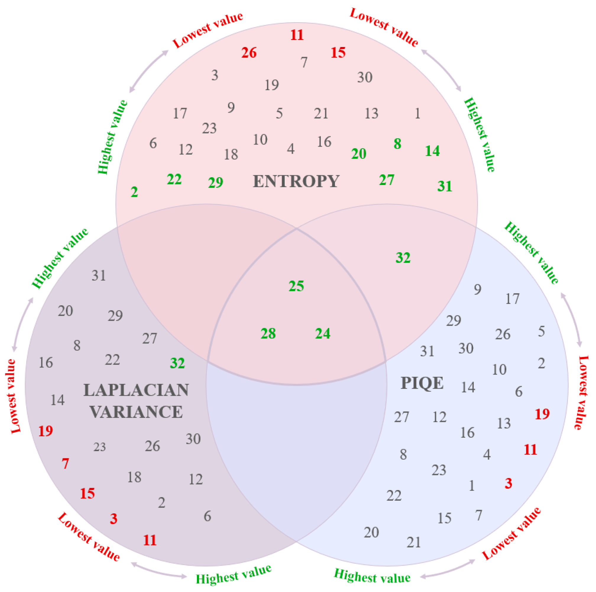
| Channel | 25 | 27 | 31 | 20 | 8 | 14 | 28 | 2 | 22 | 24 | 32 | 29 | 11 | 26 | 15 |
|---|---|---|---|---|---|---|---|---|---|---|---|---|---|---|---|
| Entropy | 0.983 | 0.990 | 1.000 | 0.905 | 0.905 | 0.905 | 0.907 | 0.918 | 0.930 | 0.940 | 0.960 | 0.965 | 0.000 | 0.207 | 0.209 |
| Quality | highest | highest | highest | highest | highest | highest | highest | highest | highest | highest | highest | highest | lowest | lowest | lowest |
| M | 0.436 | 0.595 | 0.367 | 0.391 | 0.444 | 0.421 | 0.438 | 0.269 | 0.690 | 0.409 | 0.342 | 0.258 | 0.273 | 0.412 | 0.278 |
| L | 0.727 | 0.600 | 0.789 | 0.714 | 0.800 | 0.818 | 0.667 | 0.789 | 0.778 | 0.692 | 0.800 | 0.696 | 0.688 | 0.650 | 0.846 |
| Channel | 32 | 27 | 29 | 24 | 28 | 25 | 31 | 23 | 11 | 15 |
|---|---|---|---|---|---|---|---|---|---|---|
| Entropy | 0.970 | 0.994 | 1.000 | 0.918 | 0.965 | 0.966 | 0.968 | 0.000 | 0.011 | 0.176 |
| Quality | highest | highest | highest | highest | highest | highest | highest | lowest | lowest | lowest |
| M | 0.367 | 0.349 | 0.463 | 0.500 | 0.302 | 0.429 | 0.400 | 0.696 | 0.375 | 0.300 |
| L | 0.733 | 0.750 | 0.773 | 0.833 | 0.800 | 0.750 | 0.810 | 0.429 | 0.800 | 0.714 |
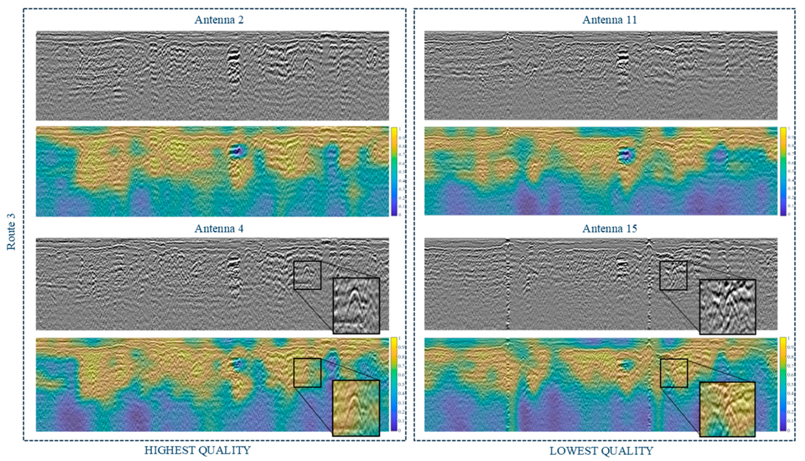
| Channel | 3 | 4 | 2 | 11 | 15 | 26 |
|---|---|---|---|---|---|---|
| Entropy | 0.907 | 0.976 | 1.000 | 0.000 | 0.084 | 0.122 |
| Quality | highest | highest | highest | lowest | lowest | lowest |
| M | 0.605 | 0.600 | 0.634 | 0.676 | 0.525 | 0.537 |
| L | 0.636 | 0.750 | 0.750 | 0.636 | 0.750 | 0.636 |
| Parameter | Laplacian Variance | Entropy | PIQE | ||||||
|---|---|---|---|---|---|---|---|---|---|
| Route No. | 1 | 2 | 3 | 1 | 2 | 3 | 1 | 2 | 3 |
| Mmax-min [%] | 16.5 | 14.7 | 17.5 | 41.7 | 20.0 | 10.9 | 13.6 | 39.3 | 16.9 |
| Mmax-average [%] | 2.8 | 9.3 | 8.3 | 28.0 | 9.3 | 1.7 | 6.9 | 28.9 | 5.9 |
| Lmax-min [%] | 4.0 | 40.5 | 17.3 | 16.8 | 40.5 | 11.4 | 10.3 | 6.7 | 11.4 |
| Lmax-average [%] | 0.5 | 9.6 | 8.5 | 9.6 | 9.6 | 2.5 | 4.7 | 6.2 | 2.5 |
Disclaimer/Publisher’s Note: The statements, opinions and data contained in all publications are solely those of the individual author(s) and contributor(s) and not of MDPI and/or the editor(s). MDPI and/or the editor(s) disclaim responsibility for any injury to people or property resulting from any ideas, methods, instructions or products referred to in the content. |
© 2025 by the authors. Licensee MDPI, Basel, Switzerland. This article is an open access article distributed under the terms and conditions of the Creative Commons Attribution (CC BY) license (https://creativecommons.org/licenses/by/4.0/).
Share and Cite
Pasternak, K.; Fryśkowska-Skibniewska, A.; Ortyl, Ł. An Adaptive Non-Reference Approach for Characterizing and Assessing Image Quality in Multichannel GPR for Automatic Hyperbola Detection. Appl. Sci. 2025, 15, 5126. https://doi.org/10.3390/app15095126
Pasternak K, Fryśkowska-Skibniewska A, Ortyl Ł. An Adaptive Non-Reference Approach for Characterizing and Assessing Image Quality in Multichannel GPR for Automatic Hyperbola Detection. Applied Sciences. 2025; 15(9):5126. https://doi.org/10.3390/app15095126
Chicago/Turabian StylePasternak, Klaudia, Anna Fryśkowska-Skibniewska, and Łukasz Ortyl. 2025. "An Adaptive Non-Reference Approach for Characterizing and Assessing Image Quality in Multichannel GPR for Automatic Hyperbola Detection" Applied Sciences 15, no. 9: 5126. https://doi.org/10.3390/app15095126
APA StylePasternak, K., Fryśkowska-Skibniewska, A., & Ortyl, Ł. (2025). An Adaptive Non-Reference Approach for Characterizing and Assessing Image Quality in Multichannel GPR for Automatic Hyperbola Detection. Applied Sciences, 15(9), 5126. https://doi.org/10.3390/app15095126