Efficient Implementation of Matrix-Based Image Processing Algorithms for IoT Applications

Abstract

This paper analyzes implementation approaches of matrix-based image processing algorithms. As an example, an image processing algorithm that provides both image compression and image denoising using random sample consensus and discrete cosine transform is analyzed. Two implementations are illustrated: one using the Blackfin processor with 32-bit fixed-point representation and the second using the convolutional neural network (CNN) accelerator in the MAX78000 microcontroller. Implementation with Blackfin can be considered a classic approach, in C language, possible on all existing microcontrollers. This implementation is improved by using two cores. The proposed implementation with the CNN accelerator is a new approach that effectively uses the dedicated accelerator for convolutional neural networks, with better results than a classical implementation. The execution time of matrix-based image processing algorithms can be reduced by using CNN accelerators already integrated in some modern microcontrollers to implement artificial intelligence algorithms. The proposed method uses CNN in a different way, not for artificial intelligence algorithms, but for matrix calculations using CNN resources effectively while maintaining the accuracy of the calculations. A comparison of these two implementations and the validation using MATLAB with 64 bits floating point representation are conducted. The obtained performance is good both in terms of quality of reconstructed image and execution time, and the performance differences between the infinite precision implementation and the finite precision implementation are small. The CNN accelerator implementation, based on matrix multiplication implemented using CNN, has a better performance suitable for Internet of Things applications.

1. Introduction and Related Work

In Internet of Things (IoT) application, both reducing the transmission bandwidth [1] and removing noise are necessary [2]. Image compression can involve algorithms, such as MPEG, but this algorithm is not able to remove the noise in the signal. Removing noise from images is quite a difficult task considering the content of the images and the possible types of noise.

An image is created by reflecting light into the camera lens and captured by the sensor, which converts the variable levels of light into digital signals for each image element (pixel). In the most common sensor, an amplifier is attached to each pixel and adjusts the output, making the image darker or brighter, respectively. The output voltage is converted using an analog-to-digital converter, where the variance in voltage to each pixel gets a binary value.

Noise represents unwanted content in an image caused by the condition existing when the image is captured: low light, slow shutter, and sensor issues [3]. Sharp and sudden disturbances could appear in the image, as well as uniform or constant disturbances. There are several noise sources. Most of the noise comes from the sensor or analog-to-digital conversion. For example, Gaussian noise is a type of sensor noise as an effect of sensor heat. Another example, the salt and pepper noise, manifests as pixels with erroneously bright values in dark parts of the image or dark values in bright parts. It is similar to dead pixels, except salt and pepper noise will produce this effect randomly. Usually, analog-to-digital conversion cause this kind of noise when transmitting images over noisy digital links. One class of denoising methods is based on filtering. Various filters are used to remove the noise in the image. However, that filter produces approximations, and the noise characteristics and the unknown positions of noised pixels may cause errors in reconstructed images. This aspect represents the motivation to develop non-filtering denoising techniques, based on the detection and reconstruction of affected pixels [3]. There are many methods to remove noise (median filtering, discrete cosine transform, wavelet transform, etc.), but each method can lead to blurring of the image or the removal of fine details from the image. On the other hand, the implementation of the noise elimination algorithm on microcontrollers with relatively limited resources and lower precision are aspects that must be studied. This paper considers an image processing algorithm that involves compressive sensing and random sample consensus. It involves the discrete cosine transform (DCT) and can be used both to compress the image and to denoise it. This approach could efficiently remove different types of noise combined. The algorithm intensively uses the matrix multiplications. In the literature is shown that sparse signals can be reconstructed from a reduced number of measurements. Digital images can be represented (for example, in a discrete cosine transform—DCT) by a small number of coefficients with significant values and can be considered as sparse or approximately sparse in this domain. Other methods have been developed in noise elimination from images, which employ sparsity [4,5,6,7,8]:

-

Weighted encoding with sparse nonlocal regularization (WESNR) based on soft impulse pixel detection, weighted encoding, and an integration of the sparsity and non-local self-similarity;

-

Block-matching 3D (BM3D) algorithm based on the grouping of similar blocks, a collaborative filtering (an adaptive filter and a two-stage average adaptive filter) by shrinkage in the transform domain, and then combining back the blocks into a two-dimensional signal;

-

Total-variation (TV) L1 methodology based on solving a minimization problem, considering that the image has a high total variation;

-

Hyperspectral denoising, using the spatio-spectral total variation;

-

Denoising algorithms based on deep learning and convolutional neural networks;

-

Variants of the traditional mean and median filters.

Recent methods for removing noise from images (based on sparse representation and including the use of neural networks) are illustrated in [9,10]. Of these, those that can be expressed in matrix form can be implemented using CNN accelerators. The compressive sensing idea is based on the sparsity of the sampled signal. Sparsity means that a discrete-time signal depends on several degrees of freedom much smaller than its finite length [11,12]. Many natural signals are sparse or compressible in the sense that they have concise representations when expressed in the proper basis or transformation $\mathit{\Psi }$. There is a duality between time and transformation domain (frequency) that expresses the idea that samples having a sparse representation in transformation domain (frequency) must be spread out in the domain in which they are acquired (time). We consider $\mathit{x}=\mathit{\psi }\mathit{C}$, where $\mathit{x}$ is an image with size $\left(W,H\right)$ pixels represented as a vector, with $N=WH$, $\mathit{\psi }$ is a matrix of size $\left(N,N\right)$ and $\mathit{C}$ is a vector of size $\left(N,1\right)$. The small coefficients $C_i$ may be discarded in the representation of $x\left(n\right)$ without much loss. The right choice of coefficients can lead both to the elimination of noise and to the compression of the image. Let $\mathit{y}$ be a vector of size $\left(N,1\right)$ with $S$ random chosen elements of $\mathit{x}$ in set $\mathit{S}$ and the rest zero elements and $\mathit{\Phi }$ a matrix of size $\left(N,N\right)$ with rows of the inverse of matrix $\mathit{\psi }$ selected by elements in set $\mathit{S}$. The coefficients can be chosen using the compressive sensing principle. The coefficients are computed as ${\mathit{C}}_{\mathbf{1}}=\mathit{\Phi }\mathit{y}$, and then, the signal is reconstructed as ${\mathit{x}}_1=\mathit{\Psi }{\mathit{C}}_1$. Vector $\mathit{y}$ will be selected so that ${\mathit{x}}_1-\mathit{x}$ is the minimum. Vector $\mathit{y}$ can be chosen using the random sampling consensus (CS-RANSAC) algorithm, which works well in the presence of relatively large numbers of disrupted pixels that will be considered as outliers. The other pixels, undisturbed or disturbed by weak noise, will be considered as inliers and will be selected by the CS-RANSAC algorithm as the consensus set. The consensus set is vector $\mathit{y}$ and will be used in compressive sensing reconstruction as explained above.

This paper analyzes a noise elimination algorithm (CS-RANSAC) based on compressing sense and RANSAC combined with DCT transform [12,13,14]. It is focused on the implementation of microcontrollers (for the IoT applications) and performance analysis (execution time and precision) to reduce the calculation time. This paper emphasizes the efficient implementation using CNN accelerators and compares it with classical implementations. The following sections will describe the algorithm in detail (Section 2), its performance with infinite precision (Section 3), the implementation of proposed algorithm using microcontrollers (Section 4), and the performances obtained using finite precision microcontrollers without accelerators (Section 5). Section 6 illustrates the implementation and the performance evaluation obtained using finite precision microcontrollers with integrated accelerators, and Section 7 presents the conclusion.

To improve the execution time, a modified algorithm that involves DCT denoising for image regions less affected by noise and the CS-RANSAC algorithm for the image regions more affected by noise can be used. To do this, a simplified algorithm to estimate the noise power can be used [15,16]. Finally, the results are shown and commented on. The conclusion is that such non-filtering denoising techniques can be applied with good performance to eliminate or reduce the noise in images and to compress the image, making it suitable for IoT applications.

2. The Algorithm Description

The above-mentioned algorithm is based on sparsity of discrete cosine transform. The CS-RANSAC algorithm is used to choose the non-noisy pixels. The DCT coefficients are determined using the compressive sensing method. The image to be processed is divided into blocks of smaller size $\left(B,B\right)$ (chosen according to the size of the two-dimensional DCT transform) and each block is processed separately. Two-dimensional DCT transforms (direct and inverse) will be calculated as matrix multiplications, considering that the block to be processed is transformed into a column vector, ${\mathit{x}}_b$ of dimensions $\left(N,1\right)$ with $N=B^2$, which will be multiplied by a matrix $\mathit{W}$ of dimensions $\left(B^2,B^2\right)$ determined by the DCT transformation matrix $\mathit{T}$ with $\mathit{W}=\mathit{T}\otimes \mathit{T}$, where $\otimes$ is the Kronecker product. DCT transform will be $\mathit{X}=\mathit{W}\mathit{x}$, and the inverse DCT transform is determined as $\mathit{x}={\mathit{W}}^{-1}\mathit{X}={\mathit{W}}^T\mathit{X}$. For each of the blocks, a subset ${\mathit{y}}_b$ of set ${\mathit{x}}_b$ with $S<B^2$ pixels are randomly chosen. Matrix $\mathit{A}$ is then determined, which contains the lines of the transpose of $\mathit{W}$ corresponding to the indices of the elements chosen from ${\mathit{x}}_b$. Using matrix $\mathit{A}$ and vector ${\mathit{y}}_b$, the first $k$ coefficients of the two-dimensional DCT transform are determined. Using these coefficients, the ${\mathit{x}}_{rb}$ vector is reconstructed, and the error between ${\mathit{x}}_b$ and ${\mathit{x}}_{rb}$ is determined. These steps are repeated until the error is small enough or the number of iterations exceeds a maximum imposed number. The last determined DCT coefficients will be the coefficients used to restore the pixels from the processed block. The algorithm is designed so that it can be implemented as efficiently as possible (both on a computer with infinite precision and on a microcontroller with fewer resources and lower precision). The critical elements for microcontroller implementation are matrix multiplication and calculation precision, especially when implementing the inverse matrix function. These aspects will be discussed in the microcontrollers’ implementation section. The algorithm is illustrated in Figure 1. In this figure, the necessary explanation has been included as comments enclosed between “/*” and “*/”. Figure 1a illustrates the core of the algorithm, and Figure 1b,c show the compressive sensing function and pseudo-inverse function, respectively.

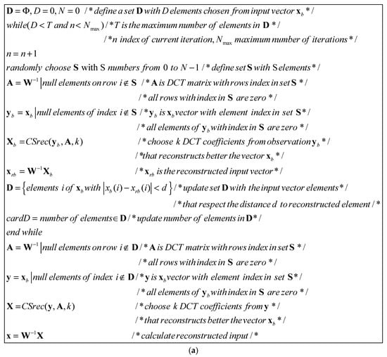
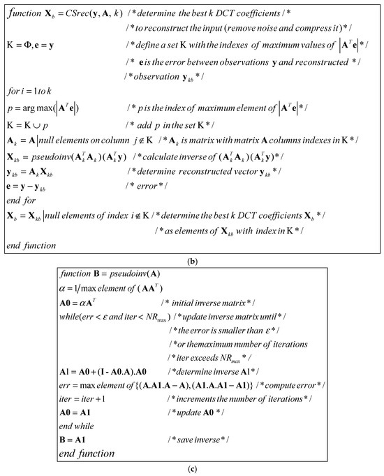
Figure 1. The CS-RANSAC algorithm. (a) CS-RANSAC algorithm (b) Compressive sensing function (c) Pseudo-inverse function.

The algorithm uses two functions:

-

The CSrec function, which receives as parameters the set of randomly chosen elements for determining non-noisy pixels, the modified transformation matrix, and the number of DCT coefficients (sparsity factor) and returns the DCT coefficients that will be used to reconstruct the elements in the block [13].

-

The pseudoinv function, which calculates the inverse of a matrix using an iterative method [17].

It was implemented in MATLAB R2024b (on a computer with an Intel I5-10210U processor at 1.60 GHz, 4 cores, 6 MB cache memory, 16 GB memory RAM, and operating system Windows 10 Pro 64-bit) in order to validate the its functionality and to evaluate the performances obtained with infinite precision.

The threshold $d$ was chosen experimentally as a tradeoff between denoising performance and computational time. The maximum number of iterations $N_{max}$ is necessary to avoid a too long running time of the algorithm in searching his convergence, and it is also set experimentally. Many images with various noise types and levels have been used to determine these two parameters as accurately as possible.

Two implementations in C language were made using the Visual DSP++ development environment for Blackfin microcontrollers and a Maxim Eclipse SDK for the MAX78000 microcontroller (Analog Devices Inc./Maxim Integrated, Wilmington, MA, USA, Digi-Key), including ARM, RISC V, and CNN cores, with 32 bits finite precision fixed point.

3. The Algorithm Performance Evaluation

This section describes the performance of the above-described algorithm in terms of the quality of the reconstructed image. The selected parameters of the algorithm were: $\mathit{B}=\mathbf{4},\mathit{S}=\mathbf{15},\mathit{k}=\mathbf{3}$. The image size was set to 512 pixels in height and 512 pixels in width [18] (for both type of implementations—MATLAB and microcontrollers). Gaussian noise, salt and pepper noise (impulsive), and multiplicative noise (speckle) were successively added to the test images. Additionally, the image was blurred. The performance of the algorithm was evaluated using the peak signal to noise ratio $\mathit{P}\mathit{S}\mathit{N}\mathit{R}=\mathbf{10}{\mathit{log}}_{\mathbf{10}}{\displaystyle \frac{{\mathbf{255}}^{\mathbf{2}}}{\frac{\mathbf{1}}{\mathit{N}\mathit{M}}{{\displaystyle \sum }}_{\mathit{i}=\mathbf{1}}^{\mathit{N}}{{\displaystyle \sum }}_{\mathit{j}=\mathbf{1}}^{\mathit{M}}{[\mathit{I}\left(\mathit{i},\mathit{j}\right)-{\mathit{I}}_{\mathit{r}}\left(\mathit{i},\mathit{j}\right)]}^{\mathbf{2}}}}$ with $\mathit{I}$ as the noisy image and ${\mathit{I}}_{\mathit{r}}$ as the reconstructed image; both dimensions $\left(\mathit{N},\mathit{M}\right)$ and the structural similarity index measure $\mathit{S}\mathit{S}\mathit{I}\mathit{M}\left(\mathit{x},\mathit{y}\right)={\displaystyle \frac{\left(\mathbf{2}{\mathit{\mu }}_x{\mathit{\mu }}_y+{\mathit{C}}_{\mathbf{1}}\right)\left(\mathbf{2}{\mathit{\sigma }}_{\mathit{x}\mathit{y}}+{\mathit{C}}_{\mathbf{2}}\right)}{\left({\mathit{\mu }}_{\mathit{x}}^{\mathbf{2}}+{\mathit{\mu }}_{\mathit{y}}^{\mathbf{2}}+{\mathit{C}}_{\mathbf{1}}\right)\left({\mathit{\sigma }}_{\mathit{x}}^{\mathbf{2}}+{\mathit{\sigma }}_{\mathit{y}}^{\mathbf{2}}+{\mathit{C}}_{\mathbf{2}}\right)}}$, where ${\mathit{\mu }}_{\mathit{x}}$, ${\mathit{\mu }}_{\mathit{y}}$, ${\mathit{\sigma }}_{\mathit{x}}^{\mathbf{2}}$, ${\mathit{\sigma }}_{\mathit{y}}^{\mathbf{2}}$, and ${\mathit{\sigma }}_{\mathit{x}\mathit{y}}$ are the mean, the variance, and the covariance of pixels in windows $x$ and $y$. The constant coefficients ${\mathit{C}}_{\mathbf{1}}$ and ${\mathit{C}}_{\mathbf{2}}$ are used to stabilize the division with a weak denominator. SSIM quantifies image quality degradation caused by data compression or by losses in data transmission. Unlike PSNR, SSIM is based on visible structures in the image and perhaps represents a more reliable indicator of image quality degradation. PSNR is an alternative measurement of the quality of the reconstructed image [19]. Figure 2, Figure 3 and Figure 4 illustrate the performance of the denoising algorithm with infinite precision (MATLAB implementation—64 bits floating point). The noise is mixed noise. The results show an image quality improvement in both PSNR (up to 6 dB) and SSIM (up to 3 times) when using the CS-RANSAC algorithm.

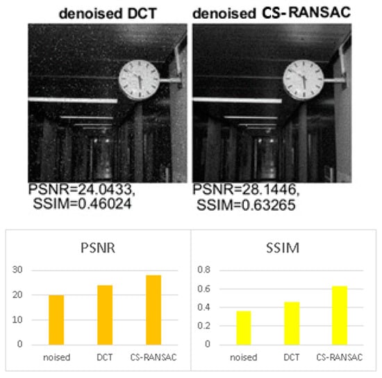
Figure 2. Performance evaluation for low noise (MATLAB implementation).

Figure 3. Performance evaluation for large noise (MATLAB implementation).

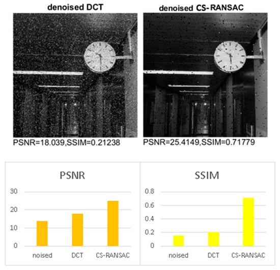
Figure 4. Performance evaluation for impulsive noise (MATLAB implementation).

In the Figure 2, the noised image has a PSNR of 20 dB and SSIM of 0.36. The noise applied on the image is mixed noise: Gaussian variance = 0.001; salt and pepper density 2%; blur kernel window length = 3; speckle variance = 0.001.

In Figure 3, the noised image has a PSNR of 17 dB and SSIM of 0.22. The noise is also mixed noise: Gaussian variance = 0.001; salt and pepper density 5%; blur kernel window length = 3; speckle variance = 0.001.

In Figure 4, the noise is impulsive with a noise density of 10%, and the noised image has a PSNR of 14 dB and SSIM of 0.15.

Table 1 summarizes the performance of the CS-RANSAC algorithm compared with DCT denoising at the same level of sparsity. One can observe that the performance is better for the CS-RANSAC algorithm both for PSNR and SSIM criteria.

Table 1. DCT denoising vs. CS-RANSAC denoising.

Noised Image		DCT Reconstructed Image		CS-RANSAC Reconstructed Image
PSNR	SSIM	PSNR	SSIM	PSNR	SSIM
20.48	0.36	24.04	0.46	28.14	0.63
17.14	0.21	20.91	0.29	26.92	0.58
14.29	0.15	18.03	0.21	25.41	0.71

A more detailed performance evaluation that proves the comparable or better performance of CS-RANSAC compared with other existing methods (BM3D, TV-L1) is given in [13]. In our paper, we evaluate the algorithm performance, in various implementation, to give a performance comparison between these implementations and to prove the possibility to implement, with good performance, relative complex image processing algorithms using microcontrollers in IoT applications.

4. The Microcontrollers’ Implementations

Two 32-bit fixed-point microcontroller (e.g., Blackfin BF5xx, and MAX7800x, Analog Devices, Analog Devices Inc./Maxim Integrated, USA, Digi-Key) implementations are proposed in this section.

The Blackfin architecture is designed for multimedia applications, the accessible memory is up to hundreds of Mbytes, and the processor clock frequency is up to 750 MHz. The instruction set is powerful (arithmetic instructions, multiplications with accumulation, dual and quad instructions, hardware loops, multifunction instructions) [20,21].

The MAX7800x chip is a dual core ultra-low power microcontroller with an ARM Cortex M4 processor with FPU up to 100 MHz with a 16 KB instruction cache, 512 KB flash memory, 128 KB SRAM, and a RISC-V Coprocessor up to 60 MHz for digital signal processing instructions. There are many interfaces (general purpose IO pins—GPIO, serial ports, analog to digital convertor (10 bit, 8 channels), neural network accelerator optimized for deep convolutional neural networks (442k 8-bit weight capacity, network depth up to 64 layers with up to 1024 channels per layer), power management for battery operations, real time clock, timers, AES 128/192/256, and CRC hardware acceleration engine. The ARM Cortex-M4 with FPU processor CM4 is well suited for the neural network system control and combines high-efficiency signal processing functionality with low energy consumption. The 32-bit RISC-V coprocessor is dedicated for ultra-low power consumption signal processing. The instructions set include: four parallel 8-bit additions/subtractions, floating point single precision operations, two parallel 16-bit additions/subtractions, two parallel MACs, 32- or 64-bit accumulate, signed, unsigned, data with or without saturation. A convolutional neural network (CNN) unit is included in the MAX7800x chip.

A more detailed architecture description of MAX 7800x, how the proposed implementation uses the CNN accelerator, and ARM and RISC V cores are shown in the next section.

The above-presented algorithm was written in C programming language, using the integrated development environment Visual DSP ++ 5.1 and Maxim Eclipse SDK. The code was automatically optimized for speed (hardware loops, interprocedural analysis) [22]. The size $S$ of set $S$ influences the performance of the algorithm. The total number of combinations (randomly chosen) for RANSAC algorithm are $C_N^S={\displaystyle \frac{N\left(N-1\right)\dots \left(N-S+1\right)}{S\left(S-1\right)\mathrm{...1}}}$. If $S$ is small, the number of combinations is large, and the algorithm may converge in many iterations (especially for large noise). If $S$ is large, the number of combinations is smaller, then the RANSAC algorithm has a smaller number of iterations. Some adaptations of the algorithm were made to reduce the execution time: for S = 15, the method of determining set S has been changed (considering that the number of possible combinations is 16, all the possible combinations will be considered and there is no need to randomly choose), and the number of iterations in the CS-RANSAC algorithm is limited to a maximum of 16 iterations. VSDP++ library functions were used for all matrix and vector operations [22,23]: matrix multiplication—matmmltf, matrix addition and subtraction—matsadd, matssub, matrix transpose—transpm, maximum and minimum element in a vector—vecmax, vecmin, location of maximum and minimum element in a vector, vecmaxloc, vecminloc. The code uses a 32-bit representation for floating point algorithm variables and computations (multiplications and additions) [23]. This approach will cause a slight decrease in precision and, therefore, the quality of the reconstructed image, but the use of a 32-bit fixed-point representation would excessively increase the execution time. The use of fixed-point representation keeps the processing time at reasonable values with an acceptable decrease in performance. The execution time was measured, in processor cycles, using the IDEs’ code profiler.

5. The Performance Using 32-Bit Fixed-Point Microcontrollers

This section describes the results obtained using the 32-bit processor. The execution time and the effect of finite precision are shown in Figure 5, Figure 6 and Figure 7. One can observe, in these figures, that the performance is good. For low and medium levels of mixed noise, the CS-RANSAC algorithm has a PSNR greater with up to 4 dB and a SSIM greater up to 80%. The SSIM obtained with CS-RANSAC is better than that of DCT even the differences in PSNR are not so high for high levels of mixed noise. The CS-RANSAC algorithm responds better for impulsive noise, as is shown in Figure 7. In Figure 5, Figure 6 and Figure 7, the noised image characteristics (PSNR, SSIM, noise type) are the same as noised images characteristics from Figure 2, Figure 3 and Figure 4.

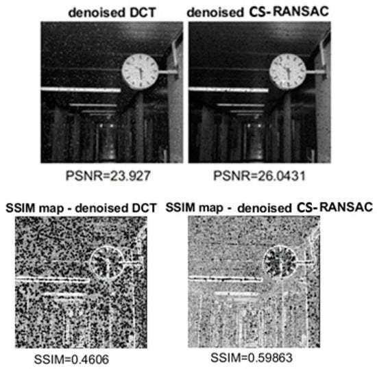
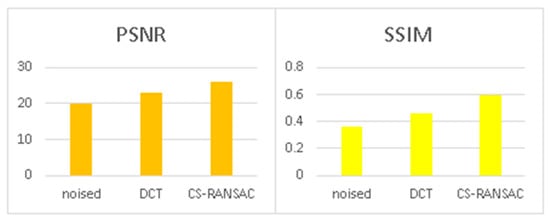
Figure 5. Performance evaluation for low noise (microcontrollers implementation).

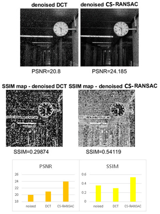
Figure 6. Performance evaluation for large noise (microcontrollers implementation).

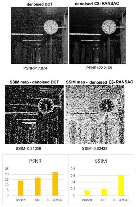
Figure 7. Performance evaluation for impulsive noise (microcontrollers implementation).

Table 2 summarizes the performances, and Table 3 compares the implementation in MATLAB with Blackfin implementation. Table 4 illustrate the execution time considering a Blackfin processor at 750 MHz.

Table 2. Performance comparison (32-bit fixed-point implementation).

Noised Image		DCT Reconstructed Image		CS-RANSAC Reconstructed Image		Execution Time CS-RANSAC Blackfin
PSNR	SSIM	PSNR	SSIM	PSNR	SSIM	Cycles	Time
20.48	0.36	23.92	0.46	26.04	0.59	4,675,862,063	6.23
17.14	0.21	20.8	0.29	24.18	0.54	5,662,802,735	7.55
14.29	0.15	17.87	0.21	22.21	0.62	8,728,624,005	11.64
15.04	0.18	18.04	0.25	19.47	0.42	7,584,207,993	10.11
19.6	0.38	22.45	0.46	23.45	0.57	4,520,337,537	6.03

Table 3. Performance comparison (32-bit fixed-point vs. MATLAB implementation).

Noised Image		DCT Reconstructed Image (Fixed Point 32 Bits)		CS-RANSAC Reconstructed Image (Fixed Point 32 Bits )		DCT Reconstructed Image (MATLAB)		CS-RANSAC Reconstructed Image (MATLAB)
PSNR	SSIM	PSNR	SSIM	PSNR	SSIM	PSNR	SSIM	PSNR	SSIM
20.48	0.36	23.92	0.46	26.04	0.59	24.04	0.46	28.14	0.63
17.14	0.21	20.8	0.29	24.18	0.54	20.91	0.29	26.92	0.58
14.29	0.15	17.87	0.21	22.21	0.62	18.03	0.21	25.41	0.71

Table 4. Execution time—seconds (32-bit fixed-point vs. MATLAB implementation).

Noised Image		Execution Time CS-RANSAC 32 Bits Fixed Point		Execution Time CS-RANSAC MATLAB
PSNR	SSIM	Cycles	Time	Time
20.48	0.36	4,675,862,063	6.23	2.49
17.14	0.21	5,662,802,735	7.55	4.79

An improved implementation using MAX7800x (with ARM core at 100 MHz, RISC V core at 60 MHz and CNN accelerator with 64 cores at 50 MHz) will be described in the next sections.

One can observe, for medium to high noise, that the execution time is reasonable (about seconds). The execution time can be decreased by using a dual-core Blackfin processor. An implementation based on an accelerator for convolutional neural networks (CNNs) is possible by implementing matrix multiplication using a 1 × 1 convolution performed with CNN.

6. The Improvement of Processing Time Using CNN Accelerator

The multiplication of two matrices $\mathit{A}=\left[a_{ij}\right]$ and $\mathit{B}=\left[b_{ij}\right]$ with the result $\mathit{C}=\mathit{A}\mathit{B}=\left[c_{ij}\right]$ and $i,j=1\dots N$ can be performed using a fully interconnected layer as in Figure 8:

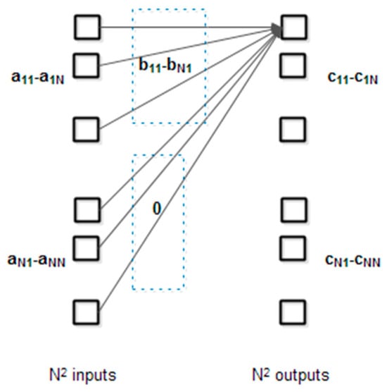
Figure 8. Neural network fully interconnected layer used for matrix multiplication.

The input layer consists of each row in matrix $\mathit{A}$ and the output layer contains the elements of the product matrix. For each input element, the weights are the corresponding elements of columns in matrix $\mathit{B}$ or zero elements. For clarity, only the weights for one output elements are shown. Figure 9 details the weights for a simple example ($N=2$):

$$\begin{array}{c}\mathit{A}=\left[\begin{array}{cc}{a}_{11}& a_{12}\\ a_{21}& a_{22}\end{array}\right]\mathrm{and}\mathit{B}=\left[\begin{array}{cc}{b}_{11}& b_{12}\\ b_{21}& b_{22}\end{array}\right]\mathrm{then}\mathit{C}=\mathit{A}\mathit{B}=\left[\begin{array}{cc}{c}_{11}& c_{12}\\ c_{21}& c_{22}\end{array}\right]=\hfill \\ \left[\begin{array}{cc}{a}_{11}{b}_{11}+a_{12}{b}_{21}& a_{11}{b}_{12}+a_{12}{b}_{22}\\ a_{21}{b}_{11}+a_{22}{b}_{21}& a_{21}{b}_{12}+a_{22}{b}_{22}\end{array}\right]\hfill \end{array}$$

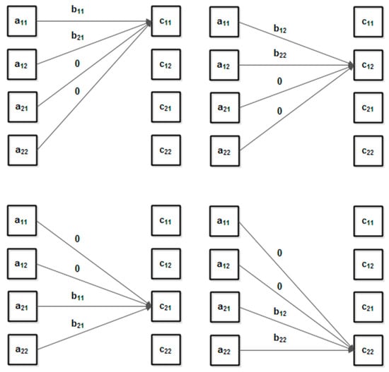
Figure 9. Neural network fully interconnected layer used for matrix multiplication (detailed example for $N=2$).

For more clarity, the weights have been shown individually for each output element.

The neural network fully interconnected layer has the output $c_{11}=a_{11}{b}_{11}+a_{12}{b}_{21}+a_{12}0+a_{12}0$ and so on. One can observe this layer outputs exactly the product matrix elements.

The implementation of the fully interconnected layer can be done in CNN by enabling the flatten mode (this mode supports a series of 1 × 1 convolution emulating a fully interconnected network with up to 1024 inputs). Matrix multiplication (fixed point) is shown in Figure 10.

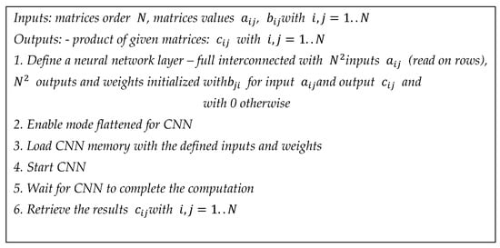
Figure 10. Matrix multiplication CNN-based algorithm (fixed point).

Using the above algorithm, a speedup about 30 times can be achieved for integer matrix multiplication, comparing with the implementation on a 32-bit fixed-point microcontroller. This can be useful for algorithms based on matrix computation that does not require a large dynamic range. In common CNNs, the values of neural network layers and weights are represented in fixed point with 8 bits. There are certain applications that require more precision. For example, the CS-RANSAC algorithm, presented in previous sections, requires higher precision due the DCT coefficients of lower order.

We proposed an approach that makes matrix multiplication with increased precision possible, considering a floating-point representation of matrix elements.

We assume that the values of matrix elements are $a_{ij}=A_{ij}{2}^{e{a}_{ij}}$, $b_{ij}=B_{ij}{2}^{e{b}_{ij}}$ and $c_{ij}=C_{ij}{2}^{e{c}_{ij}}$ with $A_{ij},B_{ij},C_{ij}$- mantises and $e{a}_{ij},e{b}_{ij},e{c}_{ij}$- exponents represented as fixed-point integers with 8 bits. The output elements are $c_{ij}={\displaystyle \sum }_{k=1}^N{A}_{ik}{2}^{e{a}_{ik}}{B}_{kj}{2}^{e{b}_{kj}}={\displaystyle \sum }_{k=1}^N{A}_{ik}{B}_{kj}{2}^{e{a}_{ik}+e{b}_{kj}}$.

The term $O_{ikj}=A_{ik}{B}_{kj}$ will be computed using a full interconnected layer, as it has been shown previously (with a slight modification of weights—see Figure 11), and the term $e{a}_{ik}+e{b}_{kj}$ will be computed using the element-wise function (the element-wise function must be enabled in CNN, and the addition function must be selected).

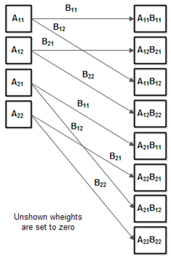
Figure 11. The full interconnected layer for floating point implementation ($N=2$).

Then, the maximum exponent is calculated as $E_{ij,max}=ma{x}_{k=1\dots N}\left(e{a}_{ik}+e{b}_{kj}\right)$, and all the terms $O_{ikj}$ will multiplied with $2^{e{a}_{ik}+e{b}_{kj}-E_{ij,max}}$ in a second full interconnected layer. The results $X_{ikj}=O_{ikj}{2}^{e{a}_{ik}+e{b}_{kj}-E_{ij,max}}$ are summed using the element wise CNN features. The sum is calculated iteratively using the element wise addition in ${\mathit{log}}_2{N}^2$ steps, as in Figure 12.

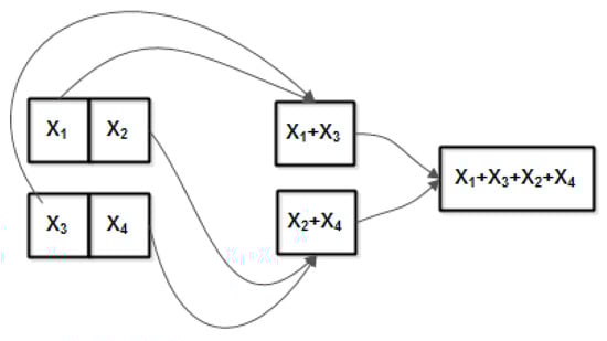
Figure 12. Element wise addition (example for $N=4$).

Finally, in a third full interconnected layer, the elements of matrix products $c_{ij}=2^{E_{ij,ma{x}_{ikj}}}$ are calculated. We assume that in image processing, one matrix (image to process) has sub-unitary mantises and $e{a}_{ij}=0,i,j=1\dots N$. The other matrix’s exponents and mantises are constant; therefore, $E_{ij,max}$ and $2^{e{a}_{ik}+e{b}_{kj}-E_{ij,max}}$ can be passed as parameters in the matrix multiplication function. The complete algorithm is illustrated in Figure 13.

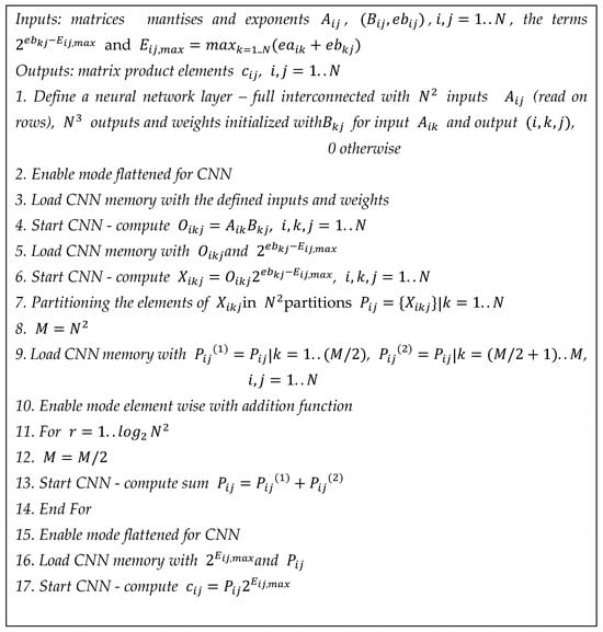
Figure 13. Matrix multiplication CNN-based algorithm (floating point).

The algorithm illustrated in Figure 13 can be efficiently implemented using the MAX78000 chip [24,25]. The block diagram of MAX7800 is illustrated in Figure 14. The CNN accelerator consists of 64 parallel processors with 512 KB of SRAM-based storage. Each processor includes a pooling unit and a convolutional engine with dedicated weight memory. Four processors share one data memory. These are further organized into groups of 16 processors that share common controls. A group of 16 processors operates as a slave to another group or independently. Data are read from SRAM associated with each processor and written to any data memory located within the accelerator. Any given processor has visibility of its dedicated weight memory and to the data memory instance it shares with the three others.

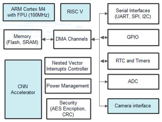
Figure 14. The MAX7800x general architecture.

In general, an algorithm (or working task) with $M$ instructions with $t_1$ average execution time per instruction can be divided into two parts: $fM$—running using one processor with $t_2$ average execution time per instruction and $\left(1-f\right)M$—running using $N$ processors with $t_3$ average execution time per instruction, with $f<1$. The speedup is calculated as $s={\displaystyle \frac{M{t}_1}{fM{t}_2+\frac{\left(1-f\right)M{t}_3}{N}}}={\displaystyle \frac{t_1}{f{t}_2+\frac{\left(1-f\right)t_3}{N}}}$. Considering $t_2=r{t}_1$ and $t_3=q{t}_1$ with $r,q<1$, the speedup becomes $s={\displaystyle \frac{t_1}{fr{t}_1+\frac{\left(1-f\right)q{t}_1}{N}}}={\displaystyle \frac{1}{fr+\frac{\left(1-f\right)q}{N}}}={\displaystyle \frac{N}{Nfr+\left(1-f\right)q}}={\displaystyle \frac{N}{f\left(Nr-q\right)+q}}$.

The term $M{t}_1$ is the computing time for single processor, and the term $fM{t}_2$ is the computing time for the non-parallelizable fraction in a multiprocessor system with $N$ processors (cores). The parallelizable fraction $\left(1-f\right)M{t}_2$ is computed on $N$ processor (cores) so the execution time will be ${\displaystyle \frac{\left(1-f\right)M{t}_2}{N}}$. All the computations involved in matrix processing (multiplication, addition) can be implemented using the CNN block in flattened or element wise modes. The above presented CS-RANSAC algorithm illustrated above was implemented using MAX78000 and its CNN accelerator. The numerical precision is similar with numerical precision obtained with previous implementation on Blackfin (the ARM and RISC cores in MAX78000 also use 32-bit fixed-point representation).

In the speedup relation, we set $N=64$ (the number of cores in CNN), $r=0.13$ (the ratio between the ARM microcontroller speed and Blackfin microcontroller), $q=0.06$ (the ratio between CNN cores speed and the Blackfin microcontroller), and $f=0.78$ (the algorithm code that does not contain matrix operations that can be performed in CNN). With this value, the theoretical speedup (between Blackfin implementation and MAX7800 implementation) is $s=9.84$. The effective speedup (obtained by counting processor cycles by the IDE code profiler) is lower due to the data transfers performed using RISC V. Figure 15 illustrates the execution time obtained with CNN implementation. In this case (software floating point implementation), the speedup obtained is about 7 times for the CS-RANSAC algorithm. The execution time depends proportionally on image size at a constant noise level because the algorithm split the images in blocks of 16 × 16 pixel, which are processed individually.

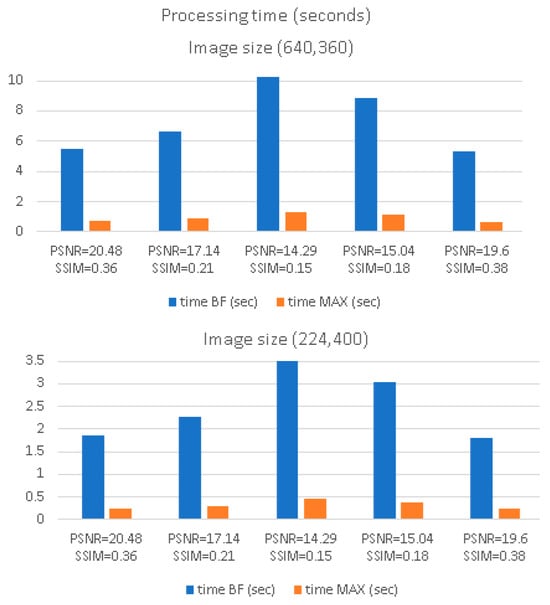
Figure 15. Processing time (various noised image sizes) for two 32-bit fixed-point implementations (Blackfin and Max78000 CNN).

The computing time of the algorithm can be improved, and modifying the way to calculate DCT coefficients using original DCT or CS-RANSAC depends on if the block is noisy or not and using the ARM and CNN in parallel.

For the first improving method, the original CS-RANSAC algorithm was combined with a noise estimator [16]. Each block is marked as light noised or heavy noised and is processed using simple DCT or CS-RANSAC, respectively. The noise estimator can be implemented in fixed point using the ARM and RISC-V microcontrollers in parallel in the MC78000 chip. Figure 16a shows how the tasks for such implementation can be scheduled.

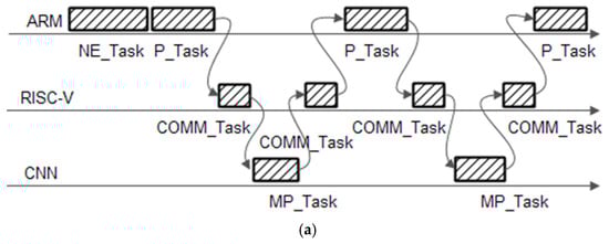
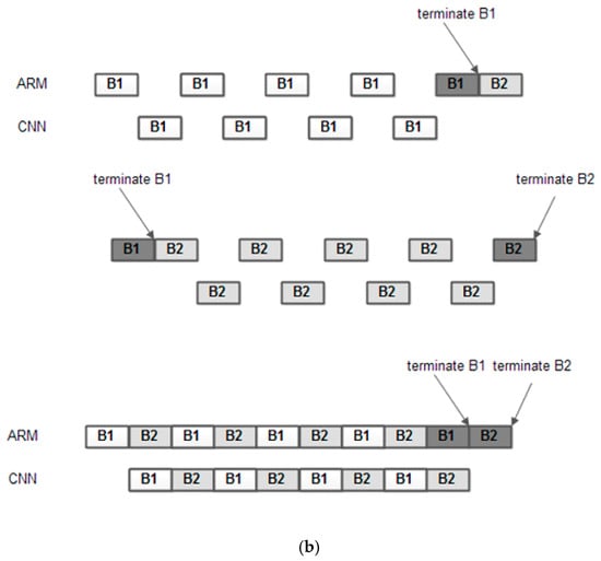
Figure 16. (a) Task scheduling for the algorithm; (b) algorithm improvement using parallel processing.

The following tasks are defined: NE_Task—for noise estimate, P_Task—the processing task that implement all the processing for DCT and CS-RANSAC noise removal and compression algorithms excepts the matrix multiplications and matrix additions, which are computed by a matrix processing task—MP_Task and COMM_task—a communication task that transfer the information (matrix values) between CNN and ARM using DMA channels. The tasks NE_Task and P_Task are running in ARM core, and the task COMM_task is running in the ARM coprocessor (that acts as a direct memory access—DMA controller). All the matrix manipulations are passed to CNN accelerator (programmed in flatten mode for matrix multiplications or element wise mode for matrix additions or subtractions) and are computed by MP_Task. All tasks are synchronized using global semaphores.

Depending on the noise level, the execution time can be reduced as illustrated in Figure 17 [26].

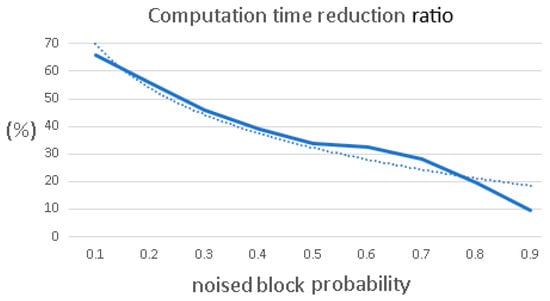
Figure 17. Computing time reduction (in dot line—trendline of ratio).

For an average noise probability of 50%, one can observe that the computation time reduction ratio is about 35%. If the noise estimator is not used, the task NE_Task in the scheduling tasks from Figure 16 is removed.

The second method ensures the halving of the computation time. This goal is achieved by partitioning the computation in matrix operations (multiplications, addition)- performed in CNN and non-matrix operations (all the remaining computations)—performed in ARM. Two blocks are processed in parallel in ARM and CNN, alternatively, as shown in Figure 16b.

For relatively small image sizes and frames per seconds, the algorithm can operate for videoclips in real time for small noise levels.

7. Conclusions

This paper focuses on the analysis of the possibility of accelerating the necessary processing in algorithms based on matrix operations. Accelerating these operations can be achieved using neural network processing units (NPUs) integrated into the architecture of today’s high-performance microcontrollers.

The aim of the work was to investigate how much the performance increases if an accelerator integrated in the microcontroller is used and under what conditions it can adapt to perform calculations not specific to the role for which it was designed. As an example, the paper presents implementations and performance analysis of an image compression and noise removal algorithm based on compressive sensing and CS-RANSAC.

This algorithm was validated as a good algorithm in terms of noise removal and image compression using infinite precision implementation (e.g., MATLAB simulations). The main goal of this work is to evaluate if a microcontroller implementation is feasible in terms of processing accuracy and computation time to be used in IoT applications that involve hardware nodes with resource constraints.

The obtained results show that good quality of the reconstructed image can be obtained for medium to relatively high noise levels (specific in IoT systems) in a calculation time of the order of seconds or tenth of seconds.

Additionally, the paper proposes methods to improve the algorithm: (1) by selectively applying DCT or the CS-RANSAC to each block in the image (without degrading the quality of the image), and (2) by using the ARM microcontroller and CNN cores in parallel or using a dual core Blackfin microcontroller.

For relatively small values (matrices of order tens), all implementations are scalable. The dimensions of the matrices are changed in code (written in C language) with only the limitation of the size of the memories in the microcontroller or CNN.

The method proposed by using CNN has certain advantages compared with a classical implementation, but it has better results for algorithms that work in fixed point. The data transfer to feed the CNN can slow down the computation time. Future research will focus on ways to organize calculations to make this data transfer more efficient and should investigate different accelerator hardware implementations and the power consumption of such implementations. Additionally, different noise models and removal noise algorithms for IoT (including static images and videoclips) will be investigate in future research.

References

- IoT Frequency Bands. Available online: https://www.data-alliance.net/blog/iot-internet-of-things-wireless-protocols-and-their-frequency-bands/ (accessed on 1 May 2024).
- Roy, A.; Bandopadhaya, S.; Chandra, S.; Suhag, A. Removal of impulse noise for multimedia-IoT applications at gateway level. Multimed. Tools Appl. 2022, 81, 34463–34480. [Google Scholar] [CrossRef]
- Bartyzel, K. Adaptive Kuwahara filter. Signal Image Video Process. 2016, 10, 663–670. [Google Scholar] [CrossRef]
- Jiang, J.; Zhang, L.; Yang, J. Mixed Noise removal by weighted encoding with sparse nonlocal regularization. IEEE Trans. Image Process. 2014, 23, 2651–2662. [Google Scholar] [CrossRef] [PubMed]
- Strong, D.; Chan, T. Edge-preserving and scale-dependent properties of total variation regularization. Inverse Probl. 2003, 19, S165–S187. [Google Scholar] [CrossRef]
- Dabov, K.; Foi, A.; Katkovnik, V.; Egiazarian, K. Image denoising by sparse 3D transform-domain collaborative filtering. IEEE Trans. Image Process. 2007, 16, 2080–2095. [Google Scholar] [CrossRef] [PubMed]
- Yang, Y.; Sun, J.; Li, H.; Xu, Z. ADMM-CSNEt: A deep learning approach for image compressive sensing. IEEE Trans. Pattern Anal. Mach. Intell. 2020, 42, 521–538. [Google Scholar] [CrossRef] [PubMed]
- Yu, G.; Sapiro, G. DCT Image Denoising: A Simple and Effective Image Denoising Algorithm. Image Process. Line 2011, 1, 292–296. [Google Scholar] [CrossRef]
- Bian, S.; He, X.; Xu, Z.; Zhang, L. Image Denoising by Deep Convolution Based on Sparse Representation. Computers 2023, 12, 112. [Google Scholar] [CrossRef]
- Mao, J.; Sun, L.; Chen, J.; Yu, S. Overview of Research on Digital Image Denoising Methods. Sensors 2025, 25, 2615. [Google Scholar] [CrossRef] [PubMed]
- Strutz, T. Data Fitting and Uncertainty (A Practical Introduction to Weighted Least Squares and Beyond), 2nd ed.; Springer Vieweg: Wiesbaden, Germany, 2016; ISBN 978-3-658-11455-8. [Google Scholar]
- Raguram, R.; Frahm, J.-M.; Pollefeys, M. A Comparative Analysis of RANSAC Techniques Leading to Adaptive Real-Time Random Sample Consensus. In Proceedings of the 10th European Conference on Computer Vision Part II, Marseille, France, 12–18 October 2008; pp. 500–513. [Google Scholar]
- Stanković, I.; Brajović, M.; Lerga, J.; Daković, M.; Stanković, L. Image denoising using RANSAC and compressive sensing. Multimedia Tools Appl. 2022, 81, 44311–44333. [Google Scholar] [CrossRef]
- Candes, E.J.; Wakin, M.B. An Introduction to Compressive Sampling. IEEE Signal Process. Mag. 2008, 25, 21–30. [Google Scholar] [CrossRef]
- Rabie, T. Robust estimation approach to blind denoising. IEEE Trans. Image Process. 2005, 14, 1755–1766. [Google Scholar] [CrossRef] [PubMed]
- Ponomarenko, M.; Gapon, N.; Voronin, V.; Egiazarian, K. Blind estimation of white Gaussian noise variance in highly textured images. Electron. Imaging 2018, 30, art00016. [Google Scholar] [CrossRef]
- A Basic Note on Iterative Matrix Inversion. Available online: https://aalexan3.math.ncsu.edu/articles/mat-inv-rep.pdf (accessed on 1 May 2024).
- TAMPERE17 Image Database. Available online: https://webpages.tuni.fi/imaging/tampere17/tampere17_grayscale.zip (accessed on 1 May 2024).
- Horé, A.; Ziou, D. Image Quality Metrics: PSNR vs. SSIM. In Proceedings of the 2010 20th International Conference on Pattern Recognition, Istanbul, Turkey, 7 October 2010; pp. 2366–2369. [Google Scholar]
- ADSP-BF533 Blackfin Processor Hardware Reference. Available online: https://www.analog.com/media/en/dsp-documentation/processor-manuals/ADSP-BF533_hwr_rev3.6.pdf (accessed on 1 May 2024).
- ADSP-BF533 EZ-KIT Lite® Evaluation System Manual. Available online: https://www.analog.com/media/en/technical-documentation/user-guides/ADSP-BF533_ezkit_man_rev.3.2.pdf (accessed on 1 May 2024).
- VisualDSP++ 5.0 C/C++ Compiler and Library Manual for Blackfin Processors. Available online: https://www.analog.com/media/en/dsp-documentation/software-manuals/50_bf_cc_rtl_mn_rev_5.4.pdf (accessed on 1 May 2024).
- Fast Floating-Point Arithmetic Emulation on Blackfin Processors. Available online: https://www.analog.com/media/en/technical-documentation/application-notes/ee.185.rev.4.08.07.pdf (accessed on 1 May 2024).
- MAX78000 Data Sheet. Available online: https://www.analog.com/media/en/technical-documentation/data-sheets/MAX78000.pdf (accessed on 1 May 2024).
- MAX78000 User Guide. Available online: https://www.analog.com/media/en/technical-documentation/user-guides/max78000-user-guide.pdf (accessed on 1 May 2024).
- Zoican, S.; Zoican, R.; Galatchi, D. Image denoising algorithm for IoT based on compressive sensing principle and Blackfin microcontrollers. In Proceedings of the 2024 15th International Conference on Communications (COMM), Bucharest, Romania, 6 November 2024; pp. 1–4. [Google Scholar] [CrossRef]
Disclaimer/Publisher’s Note: The statements, opinions and data contained in all publications are solely those of the individual author(s) and contributor(s) and not of MDPI and/or the editor(s). MDPI and/or the editor(s) disclaim responsibility for any injury to people or property resulting from any ideas, methods, instructions or products referred to in the content. |
© 2025 by the authors. Licensee MDPI, Basel, Switzerland. This article is an open access article distributed under the terms and conditions of the Creative Commons Attribution (CC BY) license (https://creativecommons.org/licenses/by/4.0/).