Article

Simulation-Guided Path Optimization for Resolving Interlocked Hook-Shaped Components

Faculty of Mechanical Engineering, Technical University of Košice, 04200 Košice, Slovakia
*
Author to whom correspondence should be addressed.
Appl. Sci. 2025, 15(9), 4944; https://doi.org/10.3390/app15094944
Submission received: 3 March 2025 / Revised: 16 April 2025 / Accepted: 27 April 2025 / Published: 29 April 2025

Abstract

:
Manipulators performing pick-and-place tasks with objects of complex shapes must consider not only how to grasp the objects but also how to maneuver them out of a bin. In this paper, we explore the industrial challenge of picking hook-shaped components, whose interlocking nature often leads to failed attempts at safely retrieving a single component at a time. Rather than explicitly modeling contact-rich interactions within optimization-based motion planners, we tackle this challenge by leveraging recent advances in sampling-based optimization and parallelizable physics simulators to predict the impact of motion on the separating subgoal, aimed at resolving interlocking. The proposed framework generates candidate trajectories initialized from a user-provided demonstration, which are then simulated and evaluated in a physics simulator to optimize robot trajectories in joint space while considering the entire planning horizon. We validate our approach through real-world experiments on a manipulator, demonstrating improved success rates in terms of separating interlocked objects compared to the industrial baseline.

1. Introduction

Due to the increasing shortage of manual labor and consumer demand, industrial robots are widely used for pick-and-place applications. These applications rely on a control pipeline consisting of several sub-steps, including object detection, approaching, grasping, transporting, and placing the object in a precise location. While controllable and predictable industrial environments simplify task and motion planning to some extent, they also present challenges in terms of desired cycle time, perception, and scalability to accommodate various object shapes. In this paper, we address the motion-planning problem of picking up hook-shaped components, such as car brake caliper brackets, which are stored unsorted in large bags. Their shape causes the components to become interlocked, often resulting in multiple components being picked simultaneously and disrupting the grasp pose due to the additional weight, see Figure 1. Consequently, the task’s success rate significantly decreases, the cycle time increases, and human intervention is required to manually separate these components.
The industrial baseline approach for pick-and-place applications is based on a finite-state machine (FSM) framework, where a user defines a sequence of high-level states. FSM is responsible for transitioning between these states based on predefined conditions or sensor feedback. Each state represents a specific action, such as a robot movement or a command for the gripper or vision system. In its simplest yet most common form, movement is defined by a set of user-specified poses relative to the object, including the pre-grasp pose, grasp pose, and post-grasp pose. This approach works well in industrial environments with simple-shaped objects. However, when dealing with more complex tasks or objects, such as ours, additional states are often introduced in the finite-state machine to handle the increased complexity. Yet, this approach becomes tedious and often still fails to account for all possible variations that may arise. On the other hand, instead of relying on predefined relative Cartesian-space waypoints, advanced motion planners enhance the robot’s capabilities and expand its range of motion [1,2]. Optimization-based planners allow for the incorporation of arbitrary aspects of behavior through constraints or objective functions. However, modeling the interlocking nature of the components studied in this paper remains a challenging task.
We propose a framework which adapts the motion required to separate the interlocked components within a pick-and-place application. Instead of explicitly optimizing dense trajectory joint-space waypoints, we simplify the optimization problem by using sparse joint position waypoints q 1 : N via . To leverage sampling-based optimization while ensuring smoothness in the sampled candidate waypoints, we interpolate them using optimal basis functions [3,4], resulting in dense, continuous candidate trajectories. Moreover, sampling-based optimization eliminates the need to design a differentiable cost term for separating the components, as it does not require gradient information. This allows us to use a parallelizable physics simulator [5] to forward-simulate candidate trajectories and predict their effects on the components’ state. The optimized motion is then used as a reference trajectory for a low-level controller.
This paper provides the following contributions:
  • A motion-planning framework for optimizing trajectories to separate interlocked hook-shaped components in a pick-and-place task.
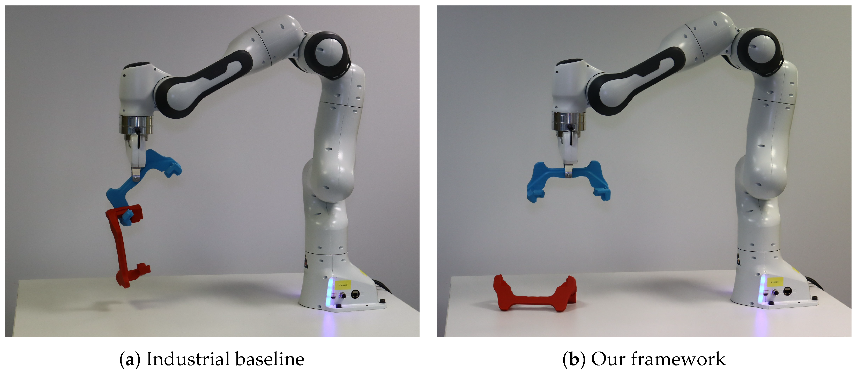
  • Real-world experimental results demonstrating that the proposed framework improves the success rate of the separating subtask compared to the industrial baseline.

2. Related Works

The majority of offline motion planners are based on either sampling or numerical optimization. Sampling-based planners [6] sample points from the configuration space of the robot to find a path between them, such as by building roadmaps [7] or incrementally growing a tree toward those sampled points [8]. In contrast, optimization-based algorithms reformulate motion planning as a mathematical program, using cost and constraint functions to capture desired motion properties. For high-dimensional systems, various methods have been developed to address non-linearities, including sequential convex optimization [1], covariant updates with Hamiltonian Monte Carlo [9], and graphs of convex sets [10]. In the context of resolving interlocked components, as addressed in this paper, such planners are particularly appealing because they enable reasoning about the separation process by encoding this task-specific objective into the optimization problem.
However, a key limitation of optimization-based planners is their reliance on cost terms and constraint functions that are continuous, differentiable, and ideally convex. In robotic applications involving high-dimensional manipulators, these functions are often non-linear and non-convex, which can lead to local minima and increased computational time. Additionally, modeling contact-rich interactions with differentiable functions is particularly challenging, especially for inexperienced users or in bin-picking scenarios where the shape of interlocked components varies frequently. This variability is also characteristic of the problem addressed in this paper, further complicating the modeling of such contact-rich interactions.
An attractive alternative is to use a class of black-box optimization algorithms that do not rely on gradient information but instead employ stochastic strategies. Their main advantage is the ability to handle non-differentiable cost terms, which simplifies the design of cost and constraint functions. Kalakrishnan et al. presented the STOMP planner [2], which generates noisy trajectory to update the candidate solution that is optimized in each iteration. By leveraging the GPU’s ability to perform parallel computing, sampling-based Model Predictive Control (MPC) methods can achieve control rates between 10 Hz and 125 Hz within a finite receding time horizon, while not requiring differentiable costs or linearization. The state-of-the-art control algorithms in this class include Model Predictive Path Integral (MPPI) [11,12] and Cross-Entropy Method (CEM) [13], which have demonstrated very fast and robust behavior, even in highly dynamic environments such as off-road autonomous driving. The STORM algorithm [14] utilizes Halton B-spline sampling and tensors to accelerate the computation of rollouts within MPPI, while ensuring the smoothness of sampled candidate trajectories. In the context of manipulators and sampling-based optimization, [4] presents the VP-STO algorithm that integrates the CMA-ES solver [15] with the trajectory representation based on optimal basis functions [3]. Our approach utilizes their idea of trajectory representation to simplify the optimization process but incorporates path integral [16] update rules. The path integral formulation has also been used in the reinforcement learning domain as Policy Improvement with path integrals (P I 2 ) to update control policies  [17], leading to its other variations, including  [18]. The path integral approach has also been used in combination with demonstrations to train visual-motion policies [19]. In the spirit of these ideas, we use a path integral formulation combined with a simple demonstration to initialize and optimize a batch of candidate strategies for separating interlocked components.
Even though these methods do not explicitly maintain gradient information, they still need to evaluate a population of candidate trajectories or actions, and perform forward simulation. This is typically achieved using mathematical modeling, which is particularly challenging for capturing the interlocking nature of our task. To address this,  [5,20] propose using generic, parallelizable physics simulators as dynamical models for MPC and MPPI, respectively, effectively eliminating the need for the aforementioned modeling. We build upon the work of [5], which uses a physics simulator for rollouts and cost evaluation. In contrast to their approach, which focuses on optimizing control inputs, we optimize entire motion paths while still leveraging the physics simulator for evaluation of the sampled candidate motions.

3. Preliminaries

In this section, we introduce the notations used in this paper and provide an overview of path integral methods and optimal basis functions, both of which are core concepts of our framework.

3.1. Notation

We consider C R n as the configuration space of the robot, where q C represents the complete specification of the robot’s n degrees of freedom (DoF), such as the joints of the robot. The joint velocities and acceleration are denoted as q ˙ , q ¨ R n , respectively. The configurations that are in collision with the environment define the set C obstacle C . By taking the difference between these two sets, we can define the set of valid configurations as C free = C C obstacle . A pose ζ is described by the transformation matrix T R 4 × 4 , which consists of a position vector p R 3 × 1 and a rotation matrix R R 3 × 3 . Transformation matrices expressed with respect to the world frame W are denoted as T W ; however, for simplicity, we will omit the W prefix, assuming that all quantities are expressed in the world frame unless specified otherwise. The sequence of end-effector poses is denoted as Ξ ee . Forces are denoted as f R 3 × 1 , representing the forces along each axis of a given frame.

3.2. Path Integral Optimization

The path integral framework [16] has its roots in quantum mechanics, and it elegantly describes particle motion as a sum of all possible trajectories a particle could take in the given space and time. Each path contributes to the particle’s behavior with a certain amplitude. The same idea has been applied to solve stochastic optimal control problems, resulting in one of the state-of-the-art control algorithms known as Model Predictive Path Integral (MPPI), as well as in the motion-planning domain [2,21]. This approach, also known as particle-based optimization [21], can be efficiently parallelized on modern GPUs, leading to faster computation times. In the context of planning, a trajectory is represented as a distribution π ϕ j represented as a set of time-indexed distributions π ϕ j , t for each timestep t along the time horizon T, such that π ϕ j = t = 0 T π ϕ j , t , where j denotes the version of the policy after j-th optimization iteration. Each distribution is parameterized by ϕ j , t , modeled as a Gaussian with a mean μ j , t and covariance matrix j , t . The full set of trajectory parameters at iteration j is thus ϕ j = { μ j , 0 : T , j , 0 : T } . In this paper, each distribution ϕ j , t corresponds to a waypoint in the joint space at timestep t. The mean μ j , t defines the nominal joint configuration, and the covariance matrix j , t captures uncertainty or exploration around that configuration. To ensure the trajectory begins and ends at fixed configurations, the first and last distributions are defined with zero variance and are centered at the initial and goal joint configurations, respectively. As a result, any sample drawn from these boundary distributions always yields the exact initial or goal joint configuration.
In the most general form, at each optimization iteration j, the algorithm samples N batch random disturbance vectors δ μ j N ( 0 , 1 ) , which are added to the current version of the policy to generate candidate actions as follows:
μ δ j , i = μ j + δ μ j , i , i [ 0 , N batch ] ,
which are used for rollouts with the system’s dynamical model to produce a corresponding batch of states x ^ i [ 0 , N batch ] , t [ 0 , T ] . The exact structure of the state x ^ mainly depends on the task-related cost terms, so it may include joint poses and velocities, end-effector poses, or even the state of objects that the robot interacts with. The candidate actions μ δ j , i represent control inputs to the dynamical model, such as joint accelerations, velocities, or, in our case, joint angles. In implementations that also update the covariance matrices, the disturbance vector δ μ j , i is sampled only once at the beginning and then scaled using the current covariance matrices j , 0 : T at each optimization iteration. In Section 4.3.1, we detail the specific method used to scale the disturbance vector used in our implementation.
Each rollout is evaluated using task-related cost terms that encourage the desired behavior of the robot, and the total cost S i [ 0 , N batch ] of the i-th rollout consists of the weighted sum of these different cost terms. To update the policy, the importance sampling weights w are computed as follows:
w i = exp ( 1 β ( S i min ( S ) ) ,
with the temperature β parameter, set to 1 in our implementation, and the cost S i of the i-th rollout that is scaled with the minimum cost from the current batch. Thereafter, each i-th rollout is weighted by w i to enforce the rollouts with higher costs to have a lower impact on the final policy update:
μ j + 1 = ( 1 α μ ) μ j + α μ i = 0 N batch w i μ δ j , i i = 0 N batch w i .
The means are updated using a sample-based gradient approximation, as in Equation (3). In the vanilla implementation, the covariance is not updated at all; however, in situations in which we want to reach the target pose, such as the manipulation domain, the covariance update, expressed in Equation (4), can lead to a more stable solution in the final configuration. Additionally, lower covariance values reduce exploration, while higher values promote it.
j + 1 = ( 1 α ) j + α i = 0 N batch w i ( μ δ j , i μ j + 1 ) ( μ δ j , i μ j + 1 ) i = 0 N batch w i
The purpose of the parameters α μ and α is to regulate the step size of the update. For additional theoretical insights, we recommend the following works [11,12,14].

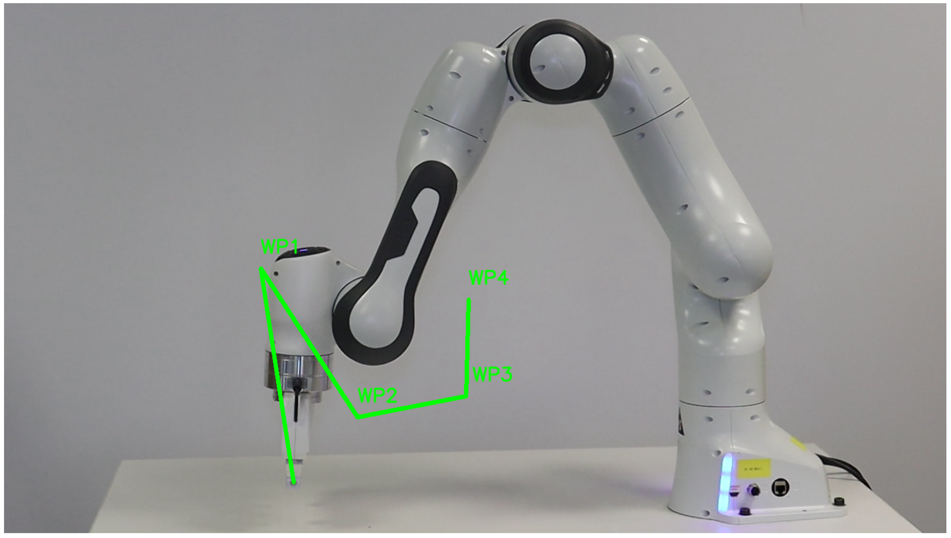
3.3. Spline Representation

We utilized the idea from [3], in which the trajectory representation is computed based on the weighted superposition of optimal basis functions Φ . The joint position spline is represented as follows:
q ( s ) = Φ ( s ) w ,
where s is a phase variable within the interval S [ 0 , 1 ] and w [ q 0 , q 1 : N v i a , q T , q ˙ 0 , q ˙ T ] is a stacked vector that consists of the initial joint position and velocity q 0 , q ˙ 0 , the target joint position and velocity q T , q ˙ T , and the sampled joint-space waypoints q 1 : N v i a . The representation ensures that an interpolated trajectory passes through all sampled waypoints while satisfying the boundary conditions, as shown in Figure 2. We always set the target joint velocity to zero. For a detailed explanation of these optimal basis functions, we highly recommend the original papers [3,4].

4. Our Approach

4.1. Problem Formulation

Consider a robotic manipulator tasked with picking and placing hook-shaped objects. This task consists of multiple subtasks within a single cycle: 1. approaching and grasping the object, 2. separating and picking it up, 3. transporting it, and 4. placing it. Each subtask requires executing a certain trajectory. The most challenging part, and the focus of this paper, is the separation subtask, which requires disengaging interlocked components. While we still solve the full pick-and-place task, the remaining subtasks can be efficiently handled using industrial baseline methods or approaches, which are explained in more detail in Section 2. Therefore, the following sections focus on the separation process rather than detailing all stages of the pick-and-place task.
Finding a trajectory to separate the components can be formulated as solving a non-linear mathematical program. The program minimizes a cost c k along the path of length T, represented by a stacked vector of joint configurations τ = [ q 0 , q 1 , , q T ] , while satisfying the required constraints. The problem can be formulated as follows:
min τ c ( τ ) , (6a) s . t . g ( q t ) 0 , t [ 0 , .… , T ] , (6b) | | f ( T ) | | σ , (6c) τ ( 0 ) = q start , τ ( T ) = q goal . (6d)
The constraint Equation (6b) represents inequality constraints that ensure joint limits and collision avoidance along a given discrete path τ are satisfied. Equation (6c) enforces that the Euclidian norm of the forces of the end-effector at the last timestep of the separating maneuver must be lower than a threshold σ , which corresponds to the maximum forces experienced when holding only one object. To ensure continuity between the separating motion and the paths of the other subtasks, the first and last joint configurations must match the grasp joint configuration, q start , from the previous subtask and the starting joint configuration, q goal , from the next one, Equation (6d).
Solving the mathematical program from Equations (6a)–(6d) requires explicitly designing differentiable constraints and modeling complex contact interactions between the robot and hook-shaped components, which is both challenging and computationally expensive. Instead, we utilize a parallelizable simulator to forward-simulate these interactions and optimize candidate trajectories, as described in the following sections.

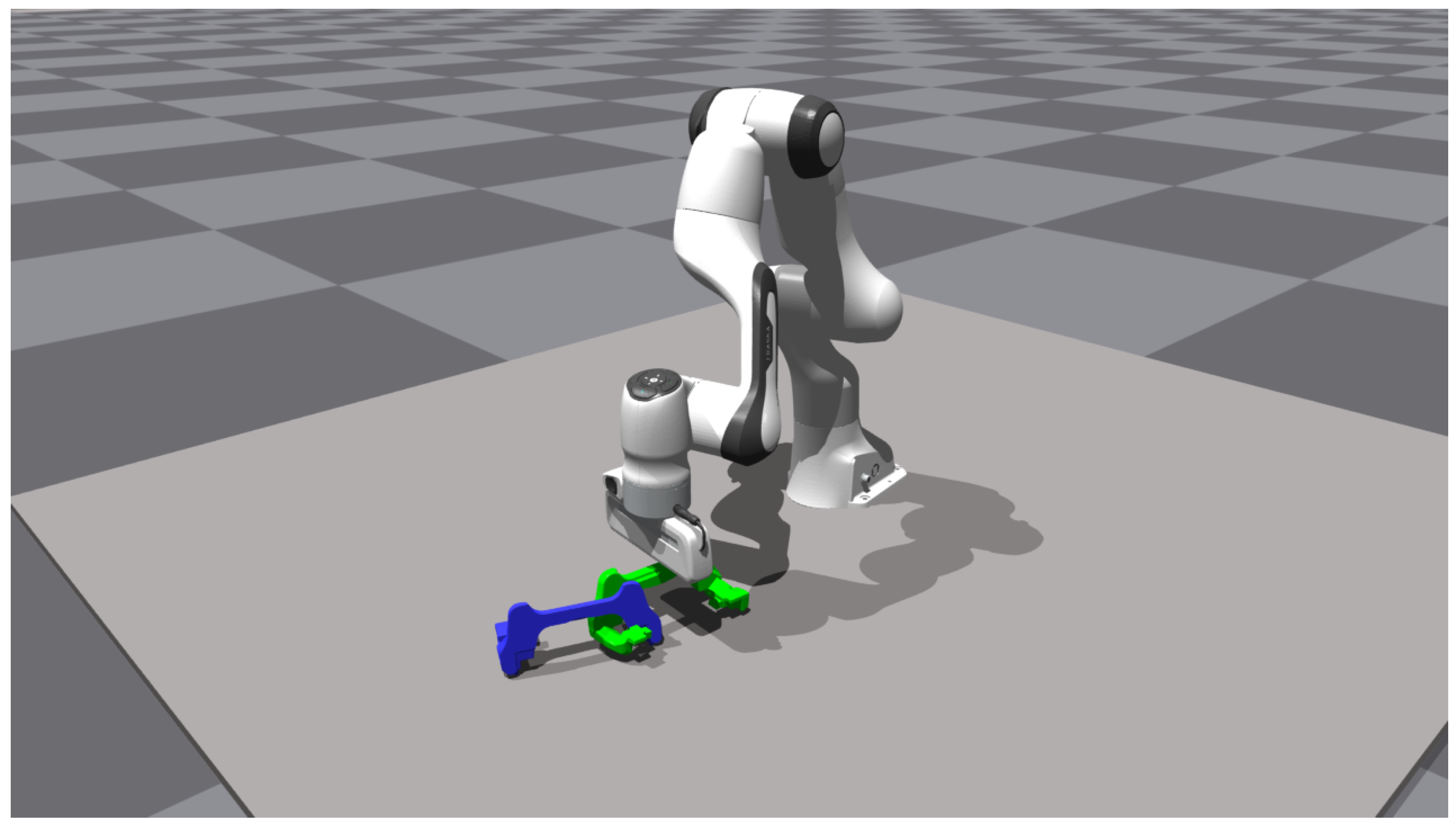
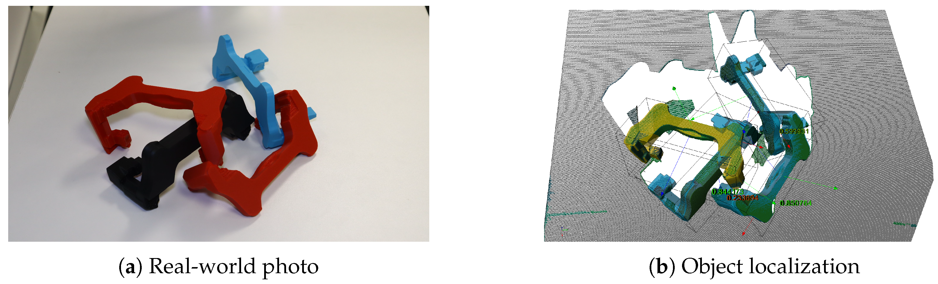
4.2. Modeling Interlocking

Using the work of [5], we utilize IsaacGym [22] as the dynamic model for rollout purposes, specifically to predict how the robot’s movements affect the task of separating components. To accomplish this, we create a simulation that represents the current state of the environment, including the robot’s joint configuration and the poses of all detected components. A straightforward approach involves forward-simulating the sequential movements for the entire pick-and-place task. This includes approaching an object, grasping it, and moving away in a manner that separates the component from the rest of the objects. However, this approach faces a significant bottleneck. To accurately simulate the contacts between the gripper and objects, the simulator must use a very small timestep, typically between 10 and 20 milliseconds or even lower, to properly capture the contact dynamics. However, this greatly increases the computational time required for rollouts. Additionally, the complex shapes of the components further exacerbate the issue by reducing the likelihood of the robot successfully grasping an object, ultimately diminishing the benefits of using the simulator.
Since we are only interested in simulating the interaction with objects during the separating stage of the pick-and-place task, we can disregard the objects’ poses in all other stages by manually placing them outside the robot’s workspace. This allows us to directly attach the component to the robot’s end-effector by extending the kinematic chain of the modeled robot through a fixed joint, as shown in Figure 3. With all components placed outside the robot’s reach, we can safely simulate the approaching or placing stages of the task without disturbing the environment or violating collision constraints with other objects. Furthermore, by assuming the robot is already holding the object at the start of the separating subtask, we eliminate the previously mentioned issue of the simulator struggling to grasp complex components, as the simulation of the grasping process is no longer required.
In the simulations, model parameters and joint limits are inherited from the robot’s URDF file, ensuring that joint limit constraints are satisfied even if a control input violates them. The inertia matrix and component mass are derived from the CAD model and incorporated into the simulator. The joints of the simulated robots are controlled by low-level position controllers.

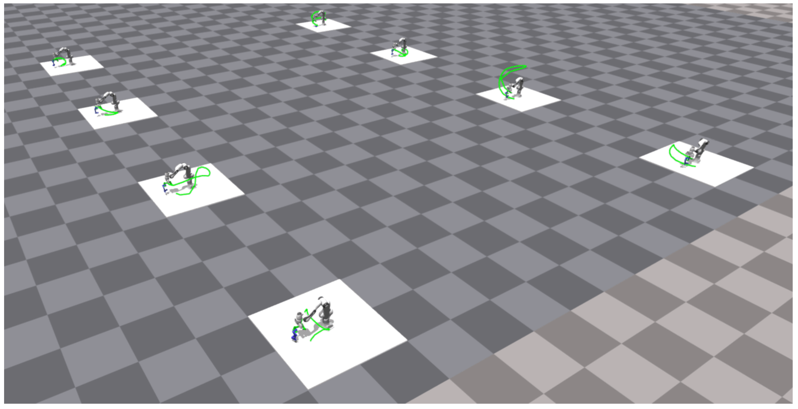
4.3. Sampling-Based Optimization

To optimize the manipulator’s path, we build upon the foundations of sampling-based MPC controllers [4,12]. We optimize the path of each subtask separately; however, they are constrained by the shared boundary conditions, as described in Equation (6d). Each path is represented by sparse joint-space waypoints q 1 : N via , which serve as waypoints between the initial and target joint configurations for a given high-level subtask. These waypoints are treated as decision variables, modeled as normal probability distributions defined by their mean and covariance matrix.

4.3.1. Sampling Noise

At the first optimization iteration, we sample noise δ μ for the waypoints from the probability distribution N ( 0 , I ) , where I is the identity matrix, to create a batch of sparse candidate paths, as described in Equation (1). To improve the smoothness of these candidates, we transform the noise δ μ using the Cholesky decomposition of the current covariance matrix via j = L j L j , which is initialized as via = R 1  [2], where R = A A is derived from the general control cost that penalizes the sum of squared accelerations. This is achieved through the finite-difference matrix A , which computes the joint acceleration as q ¨ = A q . At each iteration, the initial noise δ μ is transformed using the Cholesky factor L j of the current covariance matrix and added to the mean, as follows:
μ δ j = μ j + δ μ L j ,
resulting in N batch sparse candidate paths expressed in the configuration space of the robot.

4.3.2. Warm-Starting

The quality of the sampled paths is heavily influenced by the quality of the initial guess used to warm-start the policy means. Our experiments revealed that linear interpolation between the start and goal joint configurations was not suitable for the separating subtask, as it fails to encode an adequate strategy or bias toward separating the components. To address this, we provide a simple demonstration, shown in Figure 4, that encourages the robot to use the table, the bottom of the bin, or objects located beneath the grasped component as tools for separation. The demonstration guides the robot to press the additional, redundant objects against the table while maintaining control of the object of interest, allowing the unwanted objects to drop onto the table. The demonstration is expressed in N via poses relative to the object, and before being used to initialize the optimization, it is transformed based on the pose of the next object to be grasped, as determined by the high-level perception system, and then converted into corresponding joint configurations using inverse kinematics [23].

4.3.3. Cost Terms

The sparse candidate paths, described in Section 4.3.1, are interpolated using the aforementioned spline representation, described in Section 3.3, yielding dense candidate trajectories consisting of N eval joint configurations that satisfy the boundary conditions. These dense trajectories are then used as reference joint configurations for robots in parallelized simulations. Since the reference configurations may violate joint limits, be obstructed by obstacles, or, in general, result in collisions with the environment, making them impossible to fully execute, we instead rely on the actual trajectories and the data provided by the simulator in the following cost terms. Each cost term is computed for the i-th rollout being evaluated.
Instead of explicitly modeling a cost term to enforce separation between the components of Equation (6c), we simply penalize the Euclidean norm of the contact forces f ee ( t ) of the end-effector, as provided by the physics simulator, at every timestep t of candidate trajectories, as follows:
c ^ sep ( t ) = | | f ee ( t ) | | 2 .
Since the end-effector frame is extended by the grasped object, as described in Section 4.2, the physics simulator is used to determine whether any additional components remain attached. Consequently, the same cost term also penalizes any contact between the end-effector and the environment, effectively serving as a collision avoidance constraint between the end-effector frame and the environment.
To avoid position joint limits, we use a discontinuous cost term that penalizes joint limit violations:
c ^ lim ( q ) = 1 + q q max , if q q max 1 + q min q , if q q min 0 otherwise .
To further optimize movement efficiency, we penalize the sum of squared joint accelerations in the same way as in covariance matrix initialization:
c ^ acc ( τ eval ) = τ eval R τ eval ,
where τ eval denotes the stacked vector of joint configurations of a given candidate trajectory.
The total cost S i for the i-th interpolated dense candidate trajectory is
S i = α acc c ^ acc ( τ eval i ) + α lim t = 1 N via c ^ lim ( q i , t ) + α sep t = 1 N via γ t c ^ sep ( t i ) ,
where α sep , α smooth , and α lim are weight parameters used to prioritize different aspects of the behavior. We use a discounted cost for the c ^ sep term, as waypoints at the beginning of the maneuver have a greater influence on achieving the separating subgoal. The discount factor γ was set to 0.95 .

4.4. Framework Pipeline

Our approach follows the standard structure of industrial pick-and-place applications, where the finite-state machine dictates the actions at each state of the high-level task. In general, whenever the robot needs to move, either the desired end-effector pose is directly set in the robot’s controller, or a motion planner generates a trajectory, which is passed as waypoints. In this section, we focus on how our framework addresses the separating subtask, which is the primary focus of this paper. However, it is important to note that the same framework is uniformly applied to all subtasks to ensure consistency. Even though Algorithm 1 summarizes only the procedure for separation, the same pseudocode applies to the remaining subtasks, with separation-specific cost terms omitted. For these other subtasks, detected objects are manually repositioned outside the robot’s workspace to effectively remove them from the scene, as detailed in Section 4.2. To improve readability, we omit explicit indices for individual rollouts within the batch, as these can be efficiently handled using tensor operations.
At the beginning of the pick-and-place cycle, the robot starts in its home configuration, allowing the vision system to take an unobstructed scan of the current state of the components. This scan provides the set of object poses T obj with respect to the world frame, as shown in Figure 5. The deterministic nature of the industrial environment simplifies the task, ensuring that this set of object poses remains unchanged even after executing the initial approach and grasping motion. The set is sorted based on the z-coordinate, ensuring that objects at the top of the stack are prioritized for picking. The pose of the highest object is processed through the inverse kinematics solver [23], which also penalizes deviations from the home configuration, to obtain the target joint configuration q T .
The user-provided demonstration, shown in Figure 4, serves as the initial guess for the mean μ via 0 representing the initial stacked vector of joint configurations τ via (Line 1). After sampling the normalized noise, we perform J optimization iterations. At the beginning of each iteration, we reset the simulation based on the current state of the robot and objects. However, the object of interest is ignored, as it is considered part of the robot’s kinematic chain (Section 4.2). Thereafter, the sampled noise is scaled by the current version of the covariance matrix to enforce smooth behavior, or, more precisely, by its Cholesky decomposition L j and then added to the current version of the mean (Line 5). Thereafter, the sparse candidate paths μ δ are interpolated into dense candidate paths using optimal basis functions (Line 6), as described in Section 3.3. These dense candidates τ eval are then used as reference joint position trajectories for parallel simulations in Isaac Gym, where each trajectory is applied in full to assess feasibility and predict the object behavior resulting from the robot’s motion. We compute the costs and weights based on the simulated data and apply the same policy update (Lines 7–9) as in path integral methods, described in Equations (3) and (4).
After J optimization iterations, we interpolate the optimized mean to obtain the reference vector of joint configurations τ ref , which is then transformed into the sequence of task-space poses Ξ ee through the forward kinematics function ϕ ee and passed to a reference tracker that determines the local end-effector goal pose ζ ee for the low-level impedance controller [24] (Lines 10–12).
Algorithm 1: Framework for separating subtask
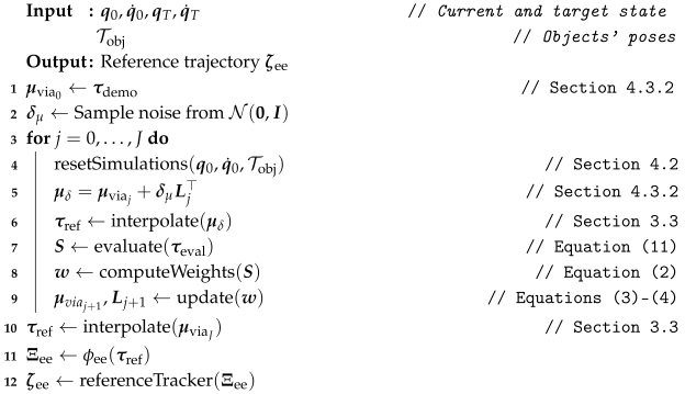
Applsci 15 04944 i001

5. Results

5.1. Experimental Setup

The presented framework is evaluated in a real-world application. We use a Franka Emika Panda 7-DoF manipulator and a Photoneo Phoxi3D Scanner M, along with their localizer package [25], to obtain accurate point clouds and component poses with an accuracy of under 2 mm . The framework was executed on a PC with an Intel Core i7-11700 K and 32 GB RAM.

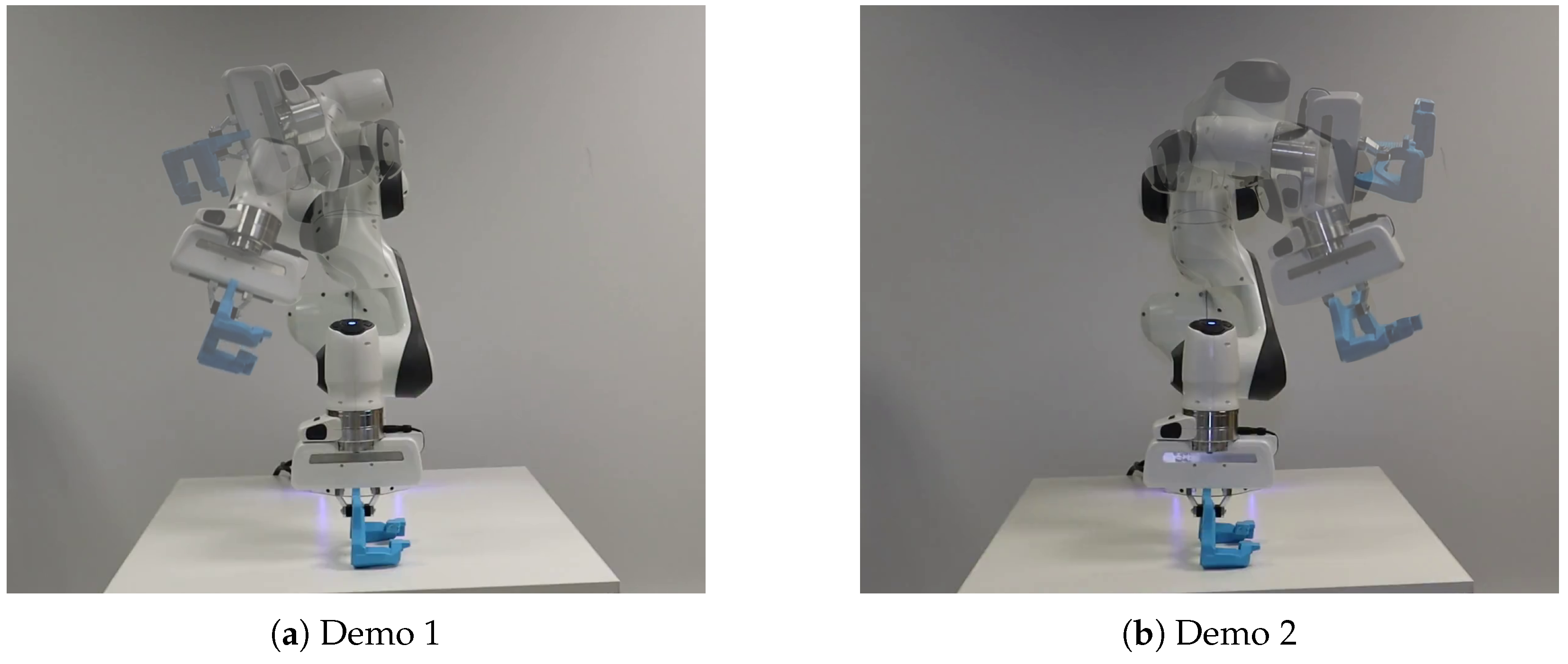
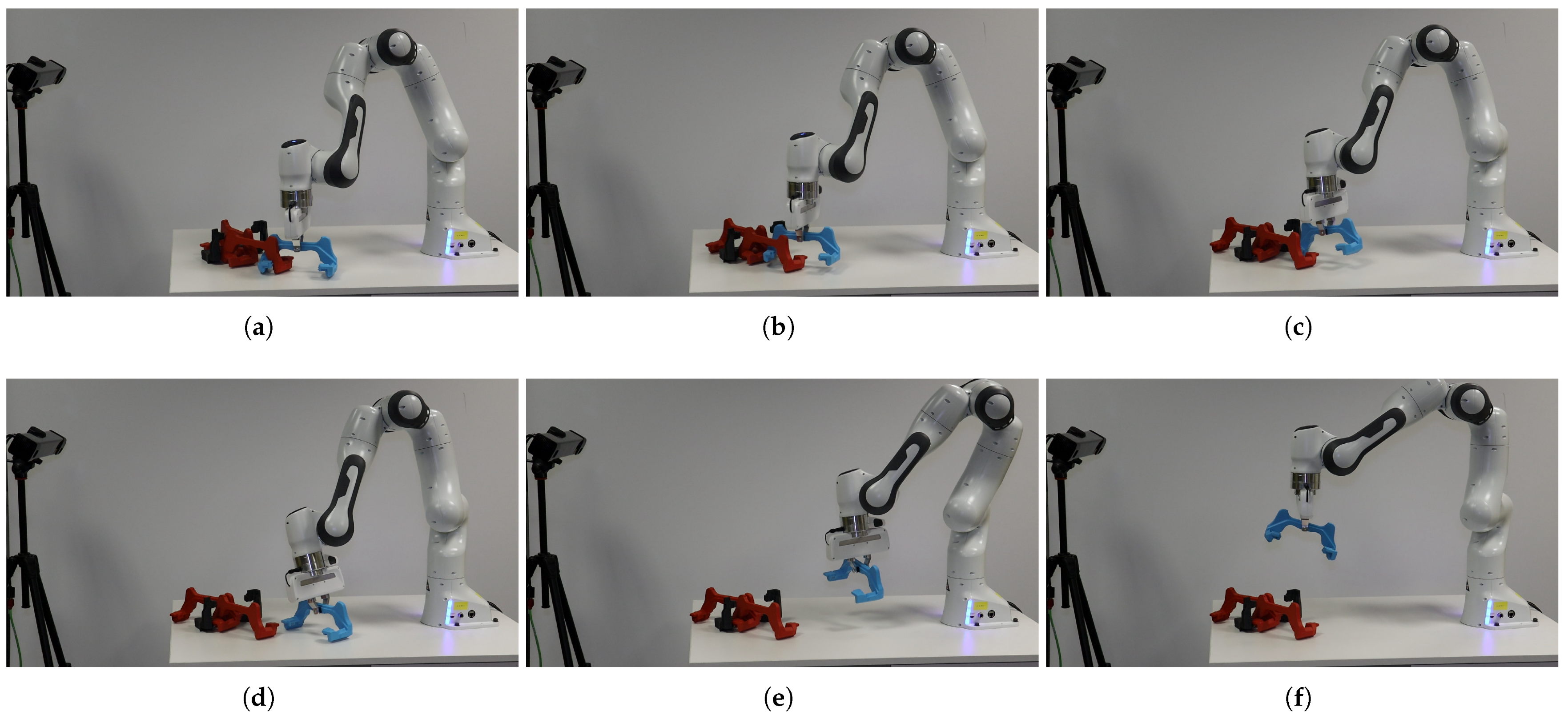
5.2. Real-World Experiments

In the real-world experiment, we compare our framework against three different demonstrations, each providing a different strategy for separating objects: Demonstration 1 and Demonstration 2 shown in Figure 6, and Demonstration 3 that we also used as an initial guess in our framework, shown in Figure 4. To evaluate sampled candidate paths, we process a batch of 500 candidates in parallel using 500 robots, as shown in Figure 7. Each candidate path consists of 4 q via waypoints, which are interpolated to 20 evaluation waypoints. The simulation timestep was set to 0.1 s. After J = 5 optimization iterations, we interpolated the optimized waypoints to 50 reference waypoints for the low-level controller. The weights were selected based on empirical tuning and set to the following values: α smooth = 10 , α lim = 1000 , α sep = 50 .
During development, we observed that a chain of interlocked components does not behave significantly differently from a pair, as additional components typically fall along with the one closest to the grasped object. In fact, resolving a longer chain can sometimes be easier, since the added weight of the extra components can assist in the separation process. We also encountered challenges with the perception pipeline, which struggled when multiple components were clustered closely together. This degradation in perception performance introduced an unintended bias in the motion planner’s behavior. To ensure a fairer comparison with minimal bias, we chose to use only two components in the comparative experiments reported in Table 1. In realistic scenarios, such as when multiple components are present on a table or in a bin, the perception pipeline often fails to detect all component poses due to occlusions caused by the top layer of the detected components. To prevent detected objects from falling in the simulation and deviating from the current state of the real-world environment, we manually added a supporting plane beneath them.
The success rate was evaluated over 10 trials, where each run was considered successful only if the robot successfully separated the object while adhering to joint limits and avoiding collisions with the environment. In each trial, the objects were manually interlocked and randomly placed within the shared workspace of the scanner and the robot to specifically investigate the separating subtask. The comparison results are shown in Table 1. We do not present the computational time for demonstrations, as the computational complexity involves only a few matrix multiplications and is therefore considered negligible. The proposed framework outperforms all other demonstrations, as each of them relies on a single strategy for resolving interlocking and therefore fails to generalize across diverse interlocked object configurations. In contrast, our framework evaluates 500 candidate motions, all originating from Demo 3. The observed failure cases were specific to our method and were primarily due to object configurations that were difficult to separate even manually, or to sim-to-real discrepancies affecting the object’s physical behavior. The second issue could potentially be addressed by introducing fallback mechanisms that safely release the grasped objects and replan the motion. The timelapse of the separating motion is shown in Figure 8.
As shown in Figure 9, after a few iterations of updating the covariance matrix, no further progress is made in updating the path, as the covariance matrix is not large enough to generate sufficiently distinct noise. This stagnation suggests that the exploration capability of the optimization process becomes constrained, preventing the discovery of potentially better solutions beyond the current path. However, since the separation motion was successfully achieved in most cases, this issue can be overlooked for the addressed application. In more complex tasks, however, this limitation could significantly impact performance and the quality of the solution. A restricted covariance matrix might lead to premature convergence to suboptimal paths, reducing the robustness of the optimization process. To address this, adaptive mechanisms for dynamically adjusting the covariance matrix size could be explored, allowing for greater variability and enhanced exploration during different stages of the optimization.

6. Conclusions

Building on recent advances in sampling-based optimization and parallelizable physics simulation, this work presents a framework for solving pick-and-place tasks involving complex hook-shaped components. The framework optimizes the paths for individual subtasks, determined by a finite-state machine, with a primary emphasis on the separating subtask, which is crucial for detaching objects from one another. We initialize the policy parameters with a simple demonstration while allowing the physics simulator to predict and evaluate the behavior of the grasped objects influenced by the robot’s movements. The proposed framework was demonstrated on a 7-DoF manipulator in a quantitative comparison against three different demonstrated strategies on how to separate the objects, outperforming all of them in terms of the success rate. The performance of our method depends on the vision system’s ability to accurately capture the scene, which presents a limitation in the proposed framework. In future work, we aim to incorporate feedback from force sensors into the perception pipeline to determine whether the robot is picking up multiple components simultaneously. This feedback could then be leveraged to enable reactive motion, leading to a higher success rate and reduced cycle time. Furthermore, integrating more advanced controllers within the simulated robots could improve the quality of candidate trajectories, expanding strategic options for more effective object separation and ultimately enhancing the efficiency of the pick-and-place process. Higher-quality candidates can reduce the number of required candidates, which may accelerate the rollout process and enable closed-loop control.

Author Contributions

Conceptualization, T.M. and R.R.; methodology, T.M. and P.J.S.; software, T.M.; experiments, T.M., P.J.S., M.K. and R.R.; 3D printing, M.V. and I.V.; writing T.M. and P.J.S., formal analysis, T.M., M.K. and I.V.; supervision, I.V. and P.J.S. All authors have read and agreed to the published version of the manuscript.

Funding

This project has received funding from the Slovak Grant Agency VEGA 1/0436/22, 008TUKE-4/2024 and 07/TUKE/2024. Views and opinions expressed are however those of the author(s) only and do not necessarily reflect those of the granting authority. The granting authority cannot be held responsible for them.

Data Availability Statement

The original contributions presented in this study are included in the article. Further inquiries can be directed to the corresponding author(s).

Conflicts of Interest

The authors declare no conflict of interest. The funders had no role in the design of the study; in the collection, analyses, or interpretation of data; in the writing of the manuscript; or in the decision to publish the results.

References

  1. Schulman, J.; Duan, Y.; Ho, J.; Lee, A.; Awwal, I.; Bradlow, H.; Pan, J.; Patil, S.; Goldberg, K.; Abbeel, P. Motion planning with sequential convex optimization and convex collision checking. Int. J. Robot. Res. 2014, 33, 1251–1270. [Google Scholar] [CrossRef]
  2. Kalakrishnan, M.; Chitta, S.; Theodorou, E.; Pastor, P.; Schaal, S. STOMP: Stochastic trajectory optimization for motion planning. In Proceedings of the 2011 IEEE International Conference on Robotics and Automation, Shanghai, China, 9–13 May 2011; pp. 4569–4574. [Google Scholar]
  3. Jankowski, J.; Racca, M.; Calinon, S. From key positions to optimal basis functions for probabilistic adaptive control. IEEE Robot. Autom. Lett. 2022, 7, 3242–3249. [Google Scholar] [CrossRef]
  4. Jankowski, J.; Brudermüller, L.; Hawes, N.; Calinon, S. Vp-sto: Via-point-based stochastic trajectory optimization for reactive robot behavior. In Proceedings of the 2023 IEEE International Conference on Robotics and Automation (ICRA), London, UK, 29 May–2 June 2023; pp. 10125–10131. [Google Scholar]
  5. Pezzato, C.; Salmi, C.; Spahn, M.; Trevisan, E.; Alonso-Mora, J.; Corbato, C.H. Sampling-based model predictive control leveraging parallelizable physics simulations. arXiv 2023, arXiv:2307.09105. [Google Scholar] [CrossRef]
  6. Kingston, Z.; Moll, M.; Kavraki, L.E. Sampling-based methods for motion planning with constraints. Annu. Rev. Control. Robot. Auton. Syst. 2018, 1, 159–185. [Google Scholar] [CrossRef]
  7. Kavraki, L.E.; Svestka, P.; Latombe, J.C.; Overmars, M.H. Probabilistic roadmaps for path planning in high-dimensional configuration spaces. IEEE Trans. Robot. Autom. 1996, 12, 566–580. [Google Scholar] [CrossRef]
  8. LaValle, S.M. Planning Algorithms; Cambridge University Press: Cambridge, UK, 2006. [Google Scholar]
  9. Ratliff, N.; Zucker, M.; Bagnell, J.A.; Srinivasa, S. CHOMP: Gradient optimization techniques for efficient motion planning. In Proceedings of the 2009 IEEE International Conference on Robotics and Automation, Kobe, Japan, 12–17 May 2009; pp. 489–494. [Google Scholar]
  10. Marcucci, T.; Petersen, M.; von Wrangel, D.; Tedrake, R. Motion planning around obstacles with convex optimization. Sci. Robot. 2023, 8, eadf7843. [Google Scholar] [CrossRef] [PubMed]
  11. Williams, G.; Drews, P.; Goldfain, B.; Rehg, J.M.; Theodorou, E.A. Aggressive driving with model predictive path integral control. In Proceedings of the 2016 IEEE International Conference on Robotics and Automation (ICRA), Stockholm, Sweden, 16–21 May 2016; pp. 1433–1440. [Google Scholar]
  12. Williams, G.; Wagener, N.; Goldfain, B.; Drews, P.; Rehg, J.M.; Boots, B.; Theodorou, E.A. Information theoretic mpc for model-based reinforcement learning. In Proceedings of the 2017 IEEE International Conference on Robotics and Automation (ICRA), Singapore, 29 May–3 June 2017; pp. 1714–1721. [Google Scholar]
  13. Pinneri, C.; Sawant, S.; Blaes, S.; Achterhold, J.; Stueckler, J.; Rolinek, M.; Martius, G. Sample-efficient cross-entropy method for real-time planning. In Proceedings of the Conference on Robot Learning, London, UK, 8–11 November 2021; pp. 1049–1065. [Google Scholar]
  14. Bhardwaj, M.; Sundaralingam, B.; Mousavian, A.; Ratliff, N.D.; Fox, D.; Ramos, F.; Boots, B. Storm: An integrated framework for fast joint-space model-predictive control for reactive manipulation. In Proceedings of the Conference on Robot Learning, Auckland, New Zealand, 14–18 December 2022; pp. 750–759. [Google Scholar]
  15. Hansen, N. The CMA evolution strategy: A tutorial. arXiv 2016, arXiv:1604.00772. [Google Scholar]
  16. Kappen, H.J. An introduction to stochastic control theory, path integrals and reinforcement learning. In AIP Conference Proceedings; American Institute of Physics: College Park, MD, USA, 2007; Volume 887, pp. 149–181. [Google Scholar]
  17. Theodorou, E.; Buchli, J.; Schaal, S. Learning policy improvements with path integrals. In Proceedings of the Thirteenth International Conference on Artificial Intelligence and Statistics. JMLR Workshop and Conference Proceedings, Sardinia, Italy, 13–15 May 2010; pp. 828–835. [Google Scholar]
  18. Stulp, F.; Sigaud, O. Path integral policy improvement with covariance matrix adaptation. arXiv 2012, arXiv:1206.4621. [Google Scholar]
  19. Chebotar, Y.; Kalakrishnan, M.; Yahya, A.; Li, A.; Schaal, S.; Levine, S. Path integral guided policy search. In Proceedings of the 2017 IEEE International Conference on Robotics and Automation (ICRA), Singapore, 29 May–3 June 2017; pp. 3381–3388. [Google Scholar]
  20. Howell, T.; Gileadi, N.; Tunyasuvunakool, S.; Zakka, K.; Erez, T.; Tassa, Y. Predictive Sampling: Real-time Behaviour Synthesis with MuJoCo. arXiv 2022, arXiv:2212.00541. [Google Scholar] [CrossRef]
  21. Sundaralingam, B.; Hari, S.K.S.; Fishman, A.; Garrett, C.; Van Wyk, K.; Blukis, V.; Millane, A.; Oleynikova, H.; Handa, A.; Ramos, F.; et al. curobo: Parallelized collision-free minimum-jerk robot motion generation. arXiv 2023, arXiv:2310.17274. [Google Scholar]
  22. Makoviychuk, V.; Wawrzyniak, L.; Guo, Y.; Lu, M.; Storey, K.; Macklin, M.; Hoeller, D.; Rudin, N.; Allshire, A.; Handa, A.; et al. Isaac gym: High performance gpu-based physics simulation for robot learning. arXiv 2021, arXiv:2108.10470. [Google Scholar]
  23. Corke, P.; Haviland, J. Not your grandmother’s toolbox–the Robotics Toolbox reinvented for Python. In Proceedings of the 2021 IEEE International Conference on Robotics and Automation (ICRA), Xi’an, China, 30 May–5 June 2021; pp. 11357–11363. [Google Scholar]
  24. Franzese, G.; Mészáros, A.; Peternel, L.; Kober, J. ILoSA: Interactive learning of stiffness and attractors. In Proceedings of the 2021 IEEE/RSJ International Conference on Intelligent Robots and Systems (IROS), Prague, Czech Republic, 27 September–1 October 2021; pp. 7778–7785. [Google Scholar]
  25. Photoneo. Photoneo. Your Partner in 3D Vision and Automation. 2025. Available online: https://www.photoneo.com/ (accessed on 23 January 2025).
Figure 1. Comparative example between the industrial baseline (a) and our framework (b) for the separating subtask. The industrial baseline does not account for interlocked components, often resulting in multiple components being picked at once. In contrast, our framework leverages predictions from the physics simulator to update the motion, effectively separating interlocked components.
Applsci 15 04944 g001
Figure 2. Example of the optimal basis function trajectory representation for q R 2 . The sampled joint-space waypoints (a) are combined with the boundary conditions to generate dense candidate trajectories (b). These dense trajectories start from the initial configuration (red point) with the desired joint velocity and terminate at the goal configuration (green point) with the specified joint velocity.
Applsci 15 04944 g002
Figure 3. Simulating interlocked objects. The green object is treated as an extension of the robot’s kinematic chain, meaning the robot is attempting to pick it up. The blue object, which is interlocked with the green one, represents the object that the robot is trying to separate from the green object.
Applsci 15 04944 g003
Figure 4. The provided demonstration establishes pressing the components against the table as the initial strategy for separating the objects. The green line shows the end-effector’s path, with the labeled Cartesian-space waypoints recomputed via inverse kinematics into joint-space configurations for the initial guess. First, the robot lifts the component to a higher position (WP1), then moves downward (WP2) to press the additional components against the table. As the robot moves back, the additional components fall back onto the table (WP3–WP4).
Applsci 15 04944 g004
Figure 5. Localizing the detected objects. The Photoneo 3D scanner captures a scan of the robot’s workspace. Using the point cloud and the CAD model of the component, it localizes the components and returns the grasp poses for each one.
Applsci 15 04944 g005
Figure 6. Demonstrations used for comparative experiments. Each strategy represents a different approach to separating objects with respect to the robot’s frame: (a) tilting the object to the right, (b) tilting the object to the left.
Applsci 15 04944 g006
Figure 7. Parallel simulations in Isaac Gym. Each robot executes a different interpolated sampled path. The different paths are represented by green lines.
Applsci 15 04944 g007
Figure 8. Selected timeframes (af) illustrating the successful extraction of the blue interlocked component from a clustered arrangement.
Applsci 15 04944 g008
Figure 9. Optimization of the end-effector’s reference trajectory in (a) X, (b) Y, and (c) Z coordinates over five optimization iterations. Each curve represents a different iteration, illustrating how the reference trajectory is adjusted in each coordinate as the optimization progresses.
Applsci 15 04944 g009
Table 1. Statistics from 10 trials involving only two interlocked objects comparing the proposed framework against three different demonstration strategies.
MethodSuccess Rate [%]Computational Time
5 Iterations [s]1 Iteration [ms]
Our802.090 ± 0.003417.2 ± 0.2
Demo 130--
Demo 230--
Demo 350--
Disclaimer/Publisher’s Note: The statements, opinions and data contained in all publications are solely those of the individual author(s) and contributor(s) and not of MDPI and/or the editor(s). MDPI and/or the editor(s) disclaim responsibility for any injury to people or property resulting from any ideas, methods, instructions or products referred to in the content.

