Real-Time Wave Energy Converter Control Using Instantaneous Frequency

Abstract

Wave Energy Converters (WECs) rely on effective Power Take-Off (PTO) control strategies to maximize energy absorption under dynamic sea conditions. Traditional hydrodynamic modeling techniques may require computationally intensive convolution calculations, making real-time control implementation challenging. This paper presents an alternative approach by leveraging instantaneous frequency estimation to dynamically adjust PTO damping in response to varying wave frequencies. Two real-time frequency estimation methods are explored: the Hilbert Transform (HT) and Phase-Locked Loop (PLL). The Hilbert Transform method provides accurate frequency tracking but introduces a delayed response due to its dependence on causal data. Conversely, the PLL approach demonstrates strong potential in frequency tracking but requires careful gain tuning, particularly in complex sea states. Comparative evaluations across multiple test cases—including sinusoidal variations, amplitude steps, frequency step changes, and real-world JONSWAP spectrum waves—highlight the strengths and limitations of each method. The two different PTO control techniques across the various frequency estimation methods were tested under real-sea states using a state-space model of a point-absorbing Wave Energy Converter. The Capture Width Ratio (CWR) is used as a performance metric, with results showing that the HT achieves a 10.6% improvement, while the PLL estimation yields a 0.9% improvement relative to the fixed parameter control baseline. These results highlight the effectiveness of real-time frequency estimation in improving energy absorption compared to static control parameters.

1. Introduction

Modeling the hydrodynamics of Wave Energy Converters (WECs) is fundamental to the development of effective control strategies. A widely adopted approach is based on the Cummins equation [1,2], which utilizes convolution integrals to account for fluid memory effects. Although accurate, this method is computationally intensive and complicates real-time determination of hydrodynamic parameters essential for optimizing Power Take-Off Unit (PTO) control.

Traditional WEC control techniques, such as passive impedance matching, typically assume a monochromatic wave environment and fixed optimal damping parameters [3]. However, real ocean conditions are broadband and irregular, making static control suboptimal. Real-time reactive control, which dynamically adjusts PTO damping based on incoming wave characteristics, offers a computationally efficient alternative better suited for such environments [4].

Recently, novel control architectures have explored the use of instantaneous frequency estimation based on the WEC’s own velocity signal rather than external wave measurements. Cantarellas et al. [5] proposed an adaptive vector control strategy that monitors the WEC velocity in real time to infer the dominant wave frequency using a Second-Order Generalized Integrator-based Frequency-Locked Loop (SOGI-FLL) structure. By tuning the PTO damping and reactance according to the estimated instantaneous velocity frequency, their method achieves maximum power absorption while mitigating large instantaneous power fluctuations.

To support real-time adaptation, various instantaneous frequency estimation methods have been explored, particularly for estimating the excitation force or surface elevation signals. Notable approaches include the Hilbert–Huang Transform (HHT) via Empirical Mode Decomposition (EMD), Frequency-Locked Loop (FLL), and Extended Kalman Filter (EKF) techniques [6]. Beyond frequency estimation, advanced control strategies have been proposed to enhance WEC performance under broadband and irregular sea conditions. For example, Giorgi et al. [7] introduced a time-varying damping control strategy, originally developed for vibration energy harvesters, which involves modulating the PTO damping coefficient at twice the wave excitation frequency to broaden the energy absorption bandwidth. They also demonstrated that the real-time adaptation of the PTO damping, even without complex predictive models, can significantly improve energy capture in irregular sea states.

Recognizing the importance of practical implementation, García-Violini et al. [8] reviewed simplified WEC control architectures based on impedance matching principles, highlighting the advantages of linear time-invariant (LTI) controllers and straightforward feedback structures suitable for embedded hardware.

Experimental validation has substantiated these theoretical findings. Fusco et al. [9] demonstrated, using the Pendulum Wave Energy Converter (PeWEC) device, that properly adapting the PTO damping in response to sea states leads to significant improvements in harvested energy. Similarly, Courtney et al. [10] confirmed that maximizing energy extraction under broadband spectra requires the real-time adjustment of the PTO force profile. These results underline the practical importance of real-time adaptive damping control and motivate the development of computationally efficient, sensor-based control approaches.

Building upon these foundations, the present work proposes a novel extension by investigating real-time instantaneous frequency estimation techniques for practical WEC control. Specifically, this study explores the application of the Hilbert Transform (HT) with median filtering and the Phase-Locked Loop (PLL) methods for real-time frequency tracking and dynamic PTO parameter adaptation.

A previous approach [11] leveraged linear wave theory and hydrodynamic datasets generated from Boundary Element Method (BEM) solvers like WAMIT [12] to express hydrodynamic coefficients as functions of instantaneous wave frequency, significantly reducing computational overhead. However, prior methods required complete future water elevation data, limiting practical real-time applicability.

This study focuses on the real-time estimation of wave surface elevation’s instantaneous frequency without requiring future data. By leveraging linear wave theory assumptions, where hydrodynamic coefficients mainly depend on wave frequency, this method enables the practical adaptation of impedance-matching control strategies for WEC systems in irregular sea conditions.

The research aims to develop implementable real-time WEC control strategies that are computationally efficient, robust under realistic conditions, and compatible with standard onboard measurements. The central hypothesis is that dynamically adapting PTO damping based on real-time frequency estimates enhances energy absorption efficiency, with precomputed frequency-dependent hydrodynamic coefficients being accurately adjusted using these estimates. Validation is achieved by demonstrating improved Capture Width Ratio compared to fixed parameter strategies.

2. Instantaneous Frequency Estimation

2.1. Signal Model

Ocean waves in real sea conditions can be modeled as a superposition of linear wave components derived from wave energy spectra such as JONSWAP and Pierson–Moskowitz [13]. These spectra describe how wave energy is distributed across different frequencies. Alternatively, the water surface elevation can be expressed as a single sinusoidal component with a time-dependent amplitude and phase.

$$x\left(t\right)=A\left(t\right)cos(\overline{\omega }t+ϵ\left(t\right)),$$

(1)

where $A\left(t\right)$ is the slowly varying envelope amplitude of the wave; $\overline{\omega }$ is the energy-weighted mean angular frequency of the wave spectrum; and $ϵ\left(t\right)$ represents the slowly varying phase.

The instantaneous frequency of the wave signal is given by the following:

$${\omega }_{\mathrm{inst}}\left(t\right)=\overline{\omega }+{\displaystyle \frac{dϵ\left(t\right)}{dt}}.$$

(2)

2.2. Hilbert Transform Approach

The first method employed for real-time instantaneous frequency estimation is the Causal Hilbert Transform (CHT). In the discrete-time domain, the analytic representation of a real signal $x\left[n\right]$ can be constructed using the Fast Fourier Transform (FFT):

$$x_{\mathrm{a}}\left[n\right]=x\left[n\right]+j\widehat{x}\left[n\right]$$

(3)

where $\widehat{x}\left[n\right]$ is the Hilbert transform of $x\left[n\right]$. The instantaneous phase $\theta \left[n\right]$ is then obtained by computing the phase angle of the analytic signal:

$$\theta \left[n\right]=\angle x_a\left[n\right]=arctan{\displaystyle \frac{\widehat{x}\left[n\right]}{x\left[n\right]}}.$$

(4)

The instantaneous frequency $\dot{\theta }\left[n\right]$ is determined by differentiating the instantaneous phase with respect to time:

$$\dot{\theta }\left[n\right]={\displaystyle \frac{\theta \left[n\right]-\theta [n-1]}{\Delta t}}.$$

(5)

To ensure practical implementation in real-time simulation, the method restricts access to only past and current water elevation data. A short-time Hilbert transform via FFT is performed within a predefined window, whose size is determined by multiplying the dominant wave peak period by a factor of 10 [14]. For example, if the dominant wave period is 9 s, then a window size of 90 s is used to compute the instantaneous frequency at each time step. The procedure is illustrated in Figure 1.

A notable challenge arises when applying FFT at the end of a data sequence, where abrupt frequency spikes may occur due to an end effect of FFT. To mitigate this issue, a median filter is introduced. The median filter processes a window of past signal values and computes the median, rather than directly using noisy endpoint data.

$$\dot{\theta }\left[n\right]:=median(\dot{\theta }[n-\delta ],\dot{\theta }[n-\delta +1],\dots ,\dot{\theta }[n-1],\dot{\theta }\left[n\right])$$

(6)

where the $\delta$ is the integer of the median window size. This effectively smooths instantaneous frequency estimation, reducing fluctuations caused by outliers. However, it introduces a slight delay in response, as the estimated value relies on past data. Despite this trade-off, the filter significantly enhances the stability and reliability of the estimated frequency.

2.3. Phase Locked Loop (PLL) Approach

PLLs are widely used in control systems to synchronize the phase and frequency of an output signal with a reference input. Their applications range from low-frequency energy systems to high-frequency communications and semiconductor devices. PLLs are generally classified into different types based on their control structures and intended applications, with Type-1 and Type-2 PLLs being the most widely studied configurations.

A Type-1 PLL consists of three key components: a phase detector (PD), a loop filter (LF), and a Voltage-Controlled Oscillator (VCO) [15]. The phase detector measures the phase difference between the input signal and the VCO output, generating an error signal. This error, processed through the loop filter, adjusts the VCO frequency to minimize the phase mismatch. Due to its simple proportional control mechanism, a Type-1 PLL is particularly well-suited for slowly varying signals, such as ocean wave propagation.

A conventional PLL consists of three key components:

• PD, which measures the phase difference between the input signal and the PLL’s output.
• LF, which filters out high-frequency noise and smooths the control signal.
• VCO, which generates an adjustable frequency to track the input signal.

For the cases analyzed in this paper, the instantaneous frequency is estimated using the enhanced PLL structure proposed by [16], as shown in Figure 2. This PLL improves phase detection and frequency tracking by directly estimating the phase and amplitude of the fundamental component of the input signal. Unlike conventional PLLs, this model directly estimates the phase and amplitude of the fundamental component of the input signal, improving robustness against noise and parameter variations. The loop filter gains were fine-tuned using the MATLAB Linearization Toolbox and PID tuner, ensuring optimal response time and robustness in tracking ocean wave frequencies.

3. Comparison of Methods

To evaluate the performance of the frequency estimation techniques, four different wave scenarios were analyzed:

• Case 1: Sinusoidal fluctuation in frequency centered around a 9 s dominant period.
• Case 2: Step change in wave amplitude, maintaining the frequency condition of Case 1.
• Case 3: A 50% step increase in frequency from the baseline 9 s condition.
• Case 4: JONSWAP sea condition with a 9 s peak period and a peak enhancement factor $\gamma =3.3$.

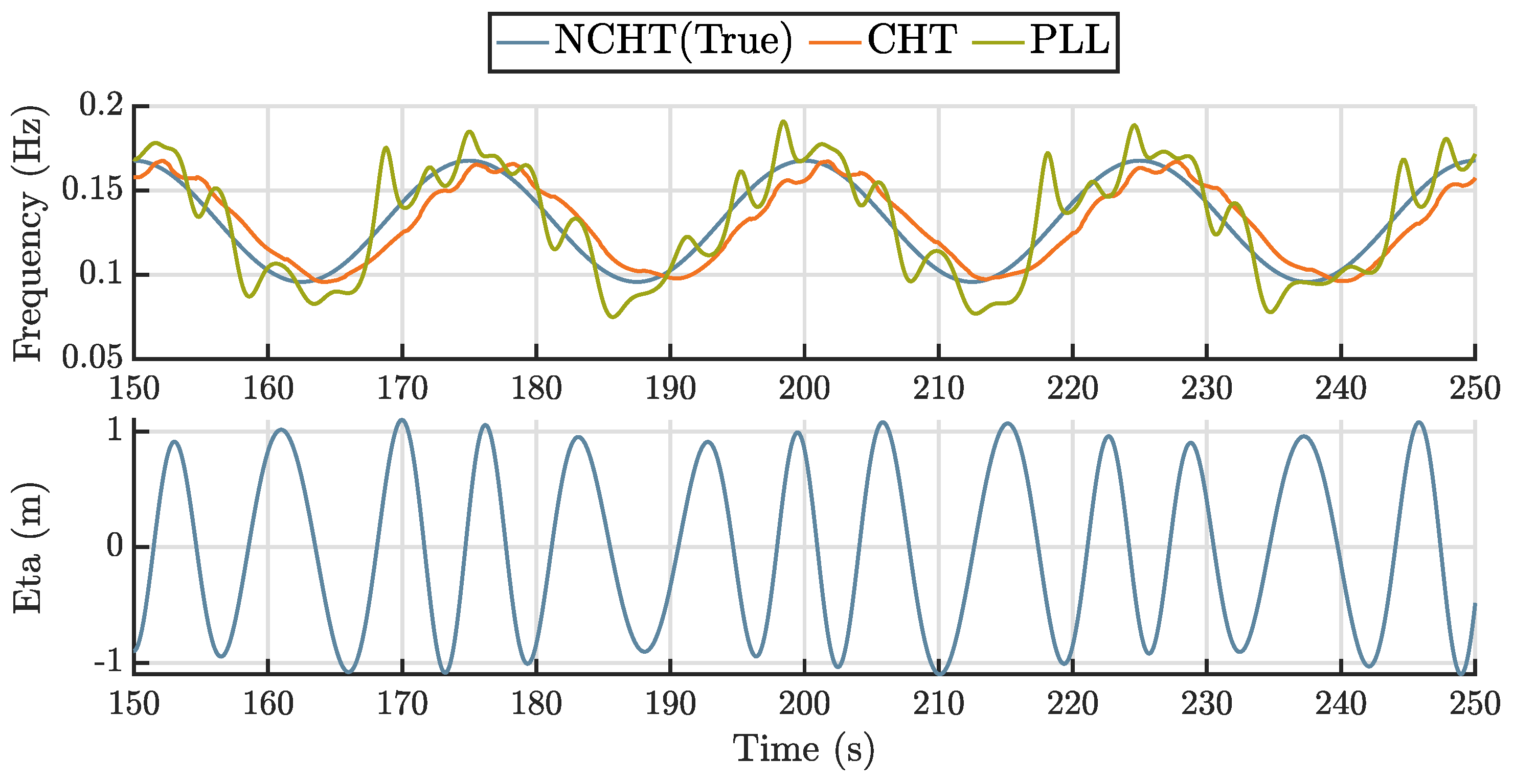
These scenarios, with simulation examples illustrated in Figure 3, Figure 4, Figure 5 and Figure 6, provide a comprehensive basis for evaluating the accuracy and robustness of each frequency estimation method. In each case, the true instantaneous frequency is compared against the estimates obtained using the CHT and PLL approaches.

3.1. NRMSE Comparison of Estimation Methods

The normalized root mean square error (NRMSE) is computed as follows:

$$\mathrm{NRMSE}={\displaystyle \frac{\sqrt{\frac{1}{N}{\sum }_{i=1}^N{(f_{\mathrm{est},i}-f_{\mathrm{true},i})}^2}}{f_{max}-f_{min}}}\times 100,$$

(7)

where $f_{\mathrm{est}}$ and $f_{\mathrm{true}}$ represent the estimated and true instantaneous frequencies, respectively, and $f_{max}$ and $f_{min}$ denote the maximum and minimum observed frequencies.

Parameter Sensitivity Analysis for Instantaneous Frequency Estimation

To determine the optimal tuning parameters for the instantaneous frequency estimation methods, an iterative parameter sweep was performed using 50 different random wave realizations. In each iteration, a JONSWAP wave elevation time series was generated over a 1200 s duration, sampled at 10 Hz. The key wave parameters were set as follows: a significant wave height of $H_s=1.5\mathrm{m}$, a peak frequency of $f_p=1/9\mathrm{Hz}$, uniformly distributed random phase information, and a spectral peakedness parameter $\gamma =3.3$.

The generated time series were characterized by an energy mean frequency $f_e$, defined as follows:

$$f_e={\displaystyle \frac{m_1}{m_0}},$$

(8)

where $m_0$ and $m_1$ are the zeroth and first spectral moments, respectively. The n-th spectral moment $m_n$ is given by the following:

$$m_n={\int }_0^{\infty }{f}^{n}S\left(f\right)df,$$

(9)

where $S\left(f\right)$ is the wave energy spectrum. Specifically, $m_0$ represents the total energy of the spectrum while $m_1$ quantifies the energy-weighted mean frequency. These spectral moments were numerically computed based on the discretized JONSWAP spectrum used in each random realization.

The resulting time series, denoted as Case 4, served as the input for both the CHT- and PLL-based instantaneous frequency estimation tests. This setup ensured that the parameter tuning was evaluated under realistic, irregular sea conditions exhibiting broadband frequency content.

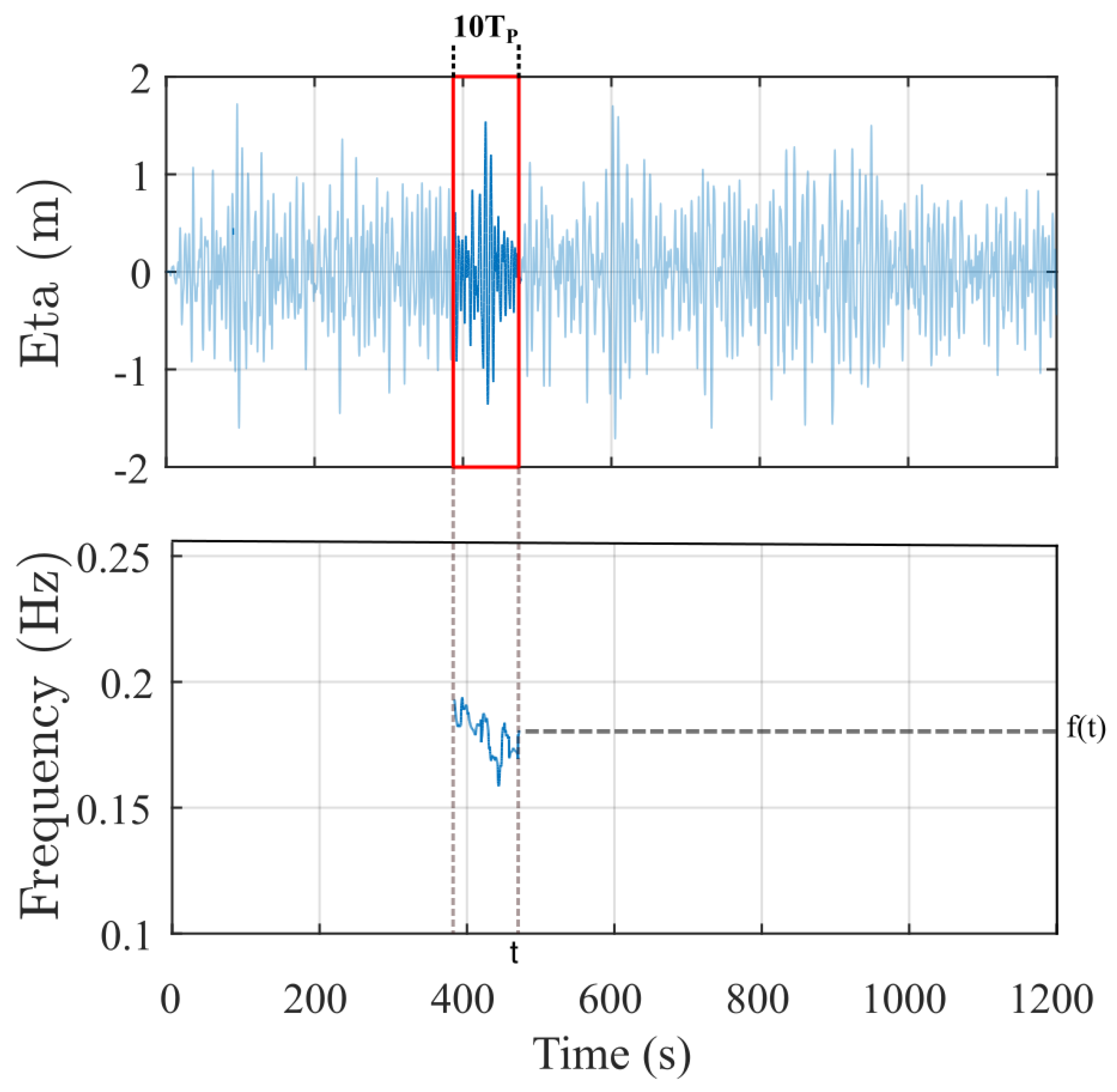
For each wave realization, the true instantaneous frequency was assumed to be computed using a Non-Causal Hilbert Transform (NCHT) algorithm, which has full access to both the past and future history of the signal. In contrast, the CHT method relies on the choice of a median window to estimate the instantaneous frequency. The median window was defined to cover approximately ten wave cycles, calculated as follows:

$$\mathrm{window}\mathrm{size}=\mathrm{round}\left({\displaystyle \frac{10}{f_e\Delta t}}\right),$$

(10)

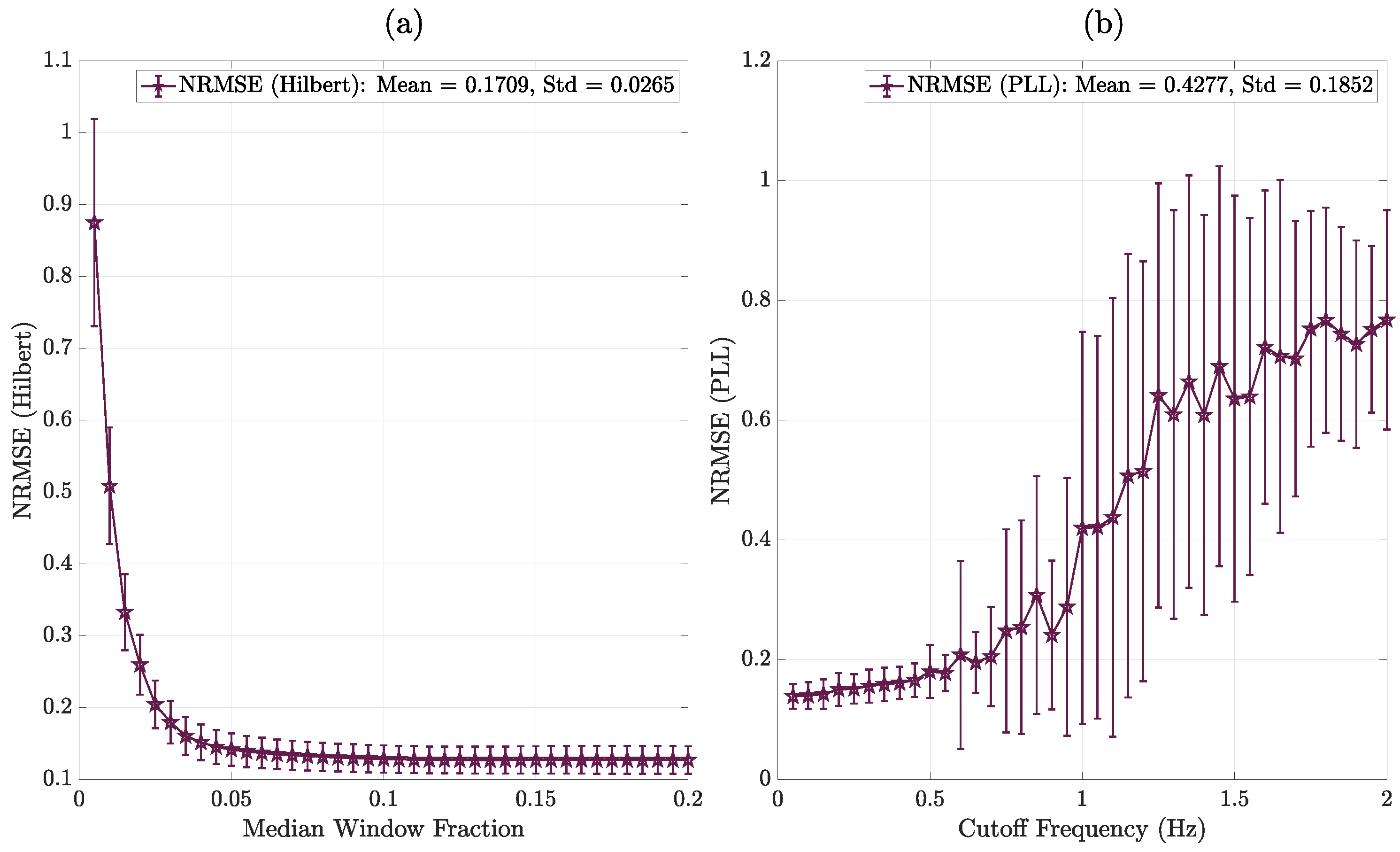
where $f_e$ is the energy mean frequency and $\Delta t$ is the simulation time step. The median window fraction is defined as the ratio of the chosen median window size to the total analysis window size. In the parameter sweep, the median window fraction was varied from 0.005 to 0.2 in increments of 0.005. For each median window fraction, the CHT-based instantaneous frequency estimate was computed, compared against the true NCHT-derived frequency (after conversion to radians per second), and the corresponding NRMSE was evaluated.

For the PLL method, the key tuning parameter is the cutoff frequency $f_c$ of the PI controller within the loop filter. The cutoff frequency was swept according to the following:

$$f_c=0.05\times i\left(\mathrm{Hz}\right),$$

(11)

where i is the sweep index, ranging from 1 to 40 (corresponding to 0.05 Hz to 2 Hz). For each cutoff frequency, the PI controller gains were tuned to maintain a fixed phase margin of $60°$, using MATLAB’s Linearization Toolbox.

For each tuning parameter value, a simulation of Case 4 was performed, and the PLL-based instantaneous frequency was estimated. This entire parameter sweep procedure was repeated for 50 independent iterations, each corresponding to different random phase information while preserving the same JONSWAP spectral.

Table 1. NRMSE comparison of CHT and PLL estimation methods.

Case Number	CHT NRMSE (%)	PLL NRMSE (%)
1	16.91	18.82
2	16.93	21.46
3	6.80	3.80
4	14.59	17.40

presents the final comparison of the optimized NRMSE values achieved by the CHT and PLL methods across different wave cases.

An analysis of the CHT and PLL methods reveals varying performance across the four test cases as shown in the Figure 7. In Cases 1 and 2, the HT method consistently achieved lower NRMSE values (16.91% and 16.93%) compared to PLL (18.82% and 21.46%). In Case 3, however, the PLL method outperformed CHT, achieving an NRMSE of 3.80% versus 6.80% for CHT. In the more challenging broadband condition of Case 4, CHT again demonstrated superior performance with an NRMSE of 14.59%, while the PLL method exhibited a slightly higher error of 17.40%. Overall, the results indicate that while the PLL method offers strong performance in sudden frequency change, the Hilbert-based method tends to provide more robust performance across a broader range of irregular wave conditions as shown in the Figure 8. Plus, the performance of the PLL is very sensitive to loop gain, while CHT is less so.

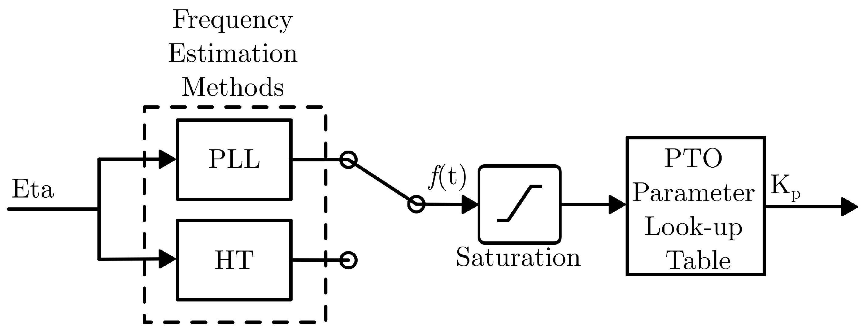
3.2. Application of Instantaneous Frequency Estimation to WEC Control

The instantaneous frequency estimation methods described in this paper—namely the CHT and the PLL—are directly applied to optimize real-time control of WECs. In the context of WEC operation, effective energy absorption is highly dependent on the dynamic matching of the PTO system impedance to the time-varying incident wave conditions. Traditional methods relying on fixed or slowly updated parameters may fail to capture the rapid fluctuations present in realistic sea states. By employing real-time instantaneous frequency estimation, the PTO damping can be continuously adjusted based on the current sea state characteristics without requiring full knowledge of future wave profiles. Specifically, the HT approach leverages past wave elevation data within a moving time window to estimate the predominant oscillation frequency, enabling the dynamic calculation of optimal PTO parameters. The PLL method, alternatively, provides a causal and computationally efficient estimation of frequency by locking onto the phase of the incoming wave signal, offering improved tracking performance under rapidly changing conditions. Through these methods, the WEC system is capable of adapting its control strategy on a wave-by-wave basis, resulting in enhanced CWR and improved overall energy harvesting efficiency compared to conventional fixed parameter designs. The proposed framework, therefore, represents a significant step toward practical, real-world WEC deployments where computational efficiency, robustness to non-stationary ocean conditions, and real-time adaptability are critical for maximizing energy capture.

4. WEC Control Using Estimated Instantaneous Frequency

4.1. WEC Control Overview

There are many WEC control approaches [17]. At the most basic level, WEC control can be considered a mechanical impedance matching problem. The WEC hydrodynamics present an intrinsic frequency-dependent combination of mass, damping, and spring behavior. Linear optimal power transfer to a PTO system is achieved when the apparent spring, mass, and damping behavior of the PTO is matched to the equivalent intrinsic mechanical impedance of the WEC. In regular sea conditions, the reactive elements of the intrinsic mechanical impedance—the mass and spring—can be combined into a single reactive element. Therefore, under regular sea conditions, optimal impedance matching can be achieved by a PTO presenting a damping and spring element, such that the damping of the PTO matches the intrinsic damping of the WEC, and the spring effect of the PTO cancels out the combined mass and spring effect of the WEC.

If the PTO is controlled to present damping (i.e., force proportional to velocity) and a spring term (i.e., force proportional to position), then it can be considered to be a form of proportional–integral (PI) control.

$$F_{pto}\left(t\right)=K_p{v}_{pto}\left(t\right)+K_i\int v_{pto}\left(t\right)dt=K_p{v}_{pto}\left(t\right)+K_i{z}_{pto}\left(t\right)$$

(12)

where $v_{pto}$ is the PTO velocity, $z_{pto}$ is the PTO position, the proportional term $K_p$ corresponds to a damping constant, and the integral term $K_i$ corresponds to a spring constant.

In the frequency domain, the mechanical impedance of this control is expressed as

$$Z_{pto}\left(\omega \right)=K_p-j{K}_i/\omega$$

(13)

Consider the WEC intrinsic mechanical impedance expressed as a frequency-dependent complex impedance $Z_i\left(\omega \right)$. Optimal impedance matching for some frequency $\widehat{\omega }$ is achieved when

$$K_p=\mathrm{Re}\left[Z_i\left(\widehat{\omega }\right)\right]$$

(14)

$$K_i=\widehat{\omega }\mathrm{Im}\left[Z_i\left(\widehat{\omega }\right)\right]$$

(15)

In some cases it is desirable for the PTO to avoid reactive power. In that case, the suboptimal control policy is

$$K_p=\sqrt{\mathrm{Re}{\left[Z_i\left(\widehat{\omega }\right)\right]}^2+\mathrm{Im}{\left[Z_i\left(\widehat{\omega }\right)\right]}^2}$$

(16)

$$K_i=0$$

(17)

In this paper, the former case, (14) and (15), which utilizes both $K_p$ and $K_i$ for full reactive control, will be referred to at PI control. The second case, (16) and (17), which utilizes only $K_p$, will be referred to as P control.

4.2. Real-Time Active PTO Control Implementation

This paper proposes a real-time impedance matching technique that leverages instantaneous frequency estimation to dynamically adjust PTO parameters [14]. Since the hydrodynamic coefficients of the WEC are frequency-dependent, the accurate estimation of the incoming wave frequency enables the real-time calculation of optimal control parameters. This ensures continuous adaptation of PTO damping and stiffness, maximizing energy extraction under varying wave conditions.

The complete real-time control process is illustrated in Figure 9. The method involves estimating the instantaneous frequency of the incoming wave using real-time signal processing techniques and then computing the optimal impedance matching parameters accordingly.

4.3. WEC Modeling

The response of a WEC is governed by its dynamic equations, which account for multiple interacting forces. Assuming the linear superposition of forces, the governing equation of motion is expressed as follows:

$$m\mathbf{a}={\mathbf{F}}_{\mathrm{ex}}+{\mathbf{F}}_{\mathrm{rad}}+{\mathbf{F}}_{\nu }+{\mathbf{F}}_{\mathrm{b}}+{\mathbf{F}}_{\mathrm{pto}},$$

(18)

where ${\mathbf{F}}_{\mathrm{ex}}$ is the excitation force due to incident waves; ${\mathbf{F}}_{\mathrm{rad}}$ is the radiation force from the body’s motion-induced waves; ${\mathbf{F}}_{\nu }$ is the viscous damping force; ${\mathbf{F}}_{\mathrm{b}}$ is the buoyancy force; and ${\mathbf{F}}_{\mathrm{pto}}$ is the Power Take-Off (PTO) force.

The hydrodynamic coefficients are used to estimate ${\mathbf{F}}_{\mathrm{ex}}$, ${\mathbf{F}}_{\mathrm{rad}}$, and ${\mathbf{F}}_{\mathrm{b}}$, which are derived using potential flow theory through BEM solvers such as WAMIT [12]. These coefficients are frequency-dependent and also influenced by the angle between the WEC body and incoming waves. However, for symmetrical geometries (e.g., cylindrical WECs), wave directionality effects can often be neglected.

A significant challenge in modeling WEC responses arises from the time-varying nature of real sea conditions. While regular waves of a single frequency can be readily simulated, real ocean waves exhibit continuously varying frequencies. To address this, Cummins’ equation [1] uses an impulse response function to model radiational hydrodynamic coefficients through convolution. Although this method provides an accurate estimation, it imposes a high computational cost due to the need for continuous integration.

An alternative approach, explored in [11], incorporates instantaneous frequency estimation to determine hydrodynamic coefficients in real sea conditions. This method effectively transforms the complex time-varying frequency problem into a regular wave problem by assigning hydrodynamic coefficients based on the momentary frequency at each time step. However, a limitation noted in [11] is that wave signals must be known in advance to compute the true instantaneous frequency, which is not feasible in real-time applications.

This paper extends the previous sections by introducing the real-time estimation of instantaneous frequency using different methods. Based on these estimations, the PTO damping coefficient, or an additional stiffness coefficient for complex conjugate control [14], is dynamically adjusted in response to varying wave frequency. This adaptive approach enhances energy absorption efficiency.

The next section presents the methodology and results, comparing the following:

• Fixed PTO damping: Tuned to the dominant wave period for baseline comparison.
• Variable PTO damping: Adaptively adjusted in real-time based on the estimated instantaneous frequency.

4.4. Capture Width Ratio (CWR)

To quantify WEC performance, the CWR is utilized as a key metric. CWR represents the ratio between the wave energy flux per unit width and the normalized power harvested by the WEC over time. The Capture Width Ratio can be thought of as somewhat analogous to the coefficient of power for a wind turbine. It is the fraction of environmental power available to the device that is converted to mechanical power.

The wave energy flux per unit width is a fundamental metric in wave energy studies, representing the transport of wave energy across a unit crest length. In deep water, where wave dispersion follows ${\sigma }^2=gk$, the wave energy flux is given by the following:

$${\overline{P}}_{\mathrm{wave}}={\displaystyle \frac{\rho g^2}{64\pi }}{H}_s^2{T}_e,$$

(19)

where $\rho =1000{\mathrm{kg}/\mathrm{m}}^3$ is the water density, $g=9.81{\mathrm{m}/\mathrm{s}}^2$ is the gravitational acceleration, $H_s$ is the significant wave height, and $T_e$ is the energy period of the wave.

This expression is derived from the general wave energy transport equation:

$${\overline{P}}_{\mathrm{wave}}=E{c}_g,$$

(20)

where $E={\displaystyle \frac{1}{16}}\rho g{H}_s^2$ is the wave energy density, and $c_g={\displaystyle \frac{g{T}_e}{4\pi }}$ is the deep-water group velocity.

By substituting these expressions and simplifying, we obtain Equation (19), which provides an analytical formulation for wave energy flux per unit width. This equation is widely used in ocean wave energy research [18].

For a JONSWAP spectrum characterized by a peak period of $T_p=9$ s, a significant wave height of $H_s=2$.4 m, a peak modulation factor of $\gamma =4$, and the energy period of $T_e\approx {\displaystyle \frac{T_p}{1.1}}=8.18$ s, the wave energy flux is computed as follows:

$${\overline{P}}_{\mathrm{wave}}\approx 22.56\mathrm{kW}/\mathrm{m}.$$

(21)

This value serves as the reference for evaluating the efficiency of WEC power absorption through the CWR.

The normalized average power captured by the PTO is expressed as follows:

$${\overline{P}}_{\mathrm{pto}}={\displaystyle \frac{E_{\mathrm{pto}}}{D_{\mathrm{WEC}}{T}_{\mathrm{sim}}}}\left(\mathrm{W}/\mathrm{m}\right),$$

(22)

where $E_{\mathrm{pto}}$ is the total energy harvested by the PTO at the end of the simulation, $D_{\mathrm{WEC}}$ is the WEC body’s diameter interacting with the incoming wave, and $T_{\mathrm{sim}}$ is the total simulation time.

The CWR is then computed as follows:

$$CWR={\displaystyle \frac{{\overline{P}}_{\mathrm{pto}}}{{\overline{P}}_{\mathrm{wave}}}}.$$

(23)

In the context of WEC performance, the CWR provides a normalized metric that quantifies how effectively a device converts available wave energy into usable mechanical power.

4.5. Fixed Parameter PTO Control

To establish a baseline for comparison and validate the effectiveness of the impedance matching technique applied to the state-space model of RM3, a period-sweeping control test was conducted. The test considers a sea state with an incoming wave spectrum characterized by a dominant period of 9 s, while the PTO control parameters are tuned separately for different assumed periods, as listed in the first column of

Table 2. CWR comparison across different control tuning periods. The incoming wave spectrum has a dominant period of 9 s, while the PTO control parameters are tuned to the values corresponding to the listed periods.

Control Period (s)	5	6	7	8	9	10	11	12
CWR (%)	14.49	19.21	22.95	24.71	24.79	23.13	19.28	12.34

.

This approach allows for the evaluation of how PTO tuning affects energy absorption when the control period does not match the actual dominant wave period. The results demonstrate that maximum energy absorption occurs when the PTO damping and stiffness parameters are tuned to match the dominant period of the incoming wave spectrum.

The implementation is performed using a state-space model of the WEC. The Simulink model used for this study is shown in Figure 10, representing the dynamics of the RM3 WEC system.

To optimize PTO control in real-time, a dedicated sub-block for optimal control estimation is designed, as illustrated in Figure 11. This block computes the optimal PTO damping and stiffness control based on the estimated instantaneous frequency, ensuring efficient energy conversion under varying wave conditions. The calculation of these parameters follows the impedance matching technique to maximize energy absorption.

To enhance stability, the real-time frequency estimate is saturated to within a range of frequencies of interest for a typical sea state, as shown in Figure 12. In Figure 11, this function is seen as the "Saturation" block in the center of the diagram.

4.5.1. Description of Estimation Methods and Control Scheme

There are four frequency estimation methods utilized:

• Fixed Parameter Control: No real-time frequency estimation is used. The PTO damping is tuned to a fixed value based on the dominant wave period.
• Phase Locked Loop (PLL)-Based Estimation: The instantaneous frequency is estimated using a PLL, which tracks phase variations to determine frequency changes dynamically.
• Causal Hilbert Transform (CHT): The CHT is applied within a short time window, providing an approximation of the instantaneous frequency using past wave data.
• Non-Causal Hilbert Transform (NCHT): The Hilbert transform is applied with full access to both past and future wave signals.

In reference to Section 4.1 and Equations (16) and (17), the control applied is simple proportional damping PTO control, in which the damping is calculated and applied at each real-time sample time in accordance with one of the frequency estimation methods described above.

4.5.2. Iteration Setup for Statistical Performance Analysis

The key parameters for the simulation setup are summarized in

Table 3. Summary of iteration setup for statistical performance analysis.

Parameter	Value/Description
Number of simulations	1000 iterations
Simulation duration	20 min per run
Time step	0.1 s
Computational platform	MacBook Pro 16″ (2021), Apple M1 Pro, MATLAB R2024b
Wave spectrum	JONSWAP spectrum
Peak enhancement factor ($\gamma$)	3.3
Significant wave height ($H_s$)	2.4 m
Peak period ($T_p$)	9 s
Phase distribution	Uniformly random in probability domain
Excitation force estimation	Convolution with IRF from WAMIT data

.

A total of 1000 independent 20 min simulations were conducted for the statistical analysis of each control approach, using a time step of 0.1 s. This relatively low sampling rate was chosen to ensure that the proposed techniques remain compatible with practical measurement systems for future experimental integration.

All simulations were performed using a MacBook Pro 16″ (2021) equipped with an Apple M1 Pro chip (Apple Inc., Cupertino, CA, USA), running MATLAB R2024b.

The wave elevation signals were generated based on a JONSWAP spectrum with a peak enhancement factor of $\gamma =3.3$, significant wave height $H_s=2.4$ m, and peak period $T_p=9$ s. These parameters were selected to ensure a consistent wave energy flux per unit width, thereby enabling a fair conditional CWR comparison across all simulations. Phase information for constructing the wave signals was assumed to be uniformly distributed in the probability domain.

The excitation force was estimated by convolution with the IRF of the excitation force, precomputed from WAMIT hydrodynamic data.

5. Results

Comparison of CWR

Table 4. Statistical summary of CWR comparison across different estimation methods and control schemes. Higher values indicate more efficient energy absorption. The percent increase over the baseline fixed parameter case is given in parentheses.

Tuning Strategy	Mean CWR %	Standard Deviation
Fixed	24.8	2.37
NCHT	25.93 (+4.6)	2.45
PLL	25.02 (+0.9)	2.84
CHT	27.42 (+10.6)	2.69

presents the CWR percentages for different estimation methods and control schemes.

The simulation results shown in Figure 13 provide insight into the comparative performance of different frequency estimation methods. Notably, the CHT-based control strategy demonstrates a more stable cumulative energy accumulation, suggesting improved consistency in energy capture over the observed period. On the other hand, both the PLL and NCHT methods are associated with higher instantaneous peak powers, which, while occasionally yielding more instantaneous absorbed power, introduce greater variability in the energy harvesting process. The time points at which significant divergence in cumulative energy occurs are under further investigation, aiming to better understand the transient dynamics introduced by different estimation techniques.

During this study, multiple parameter sweep tests were conducted using the RM3 SS model. First, the estimation parameters were varied, including the median filter window sizes for the CHT method and the cross-over frequencies of the PLL loop filter, while maintaining a fixed phase margin of 60 degrees. Second, the saturation block window sizes were adjusted, with the lower saturation limit set to $0.01 \times f_p$, where $f_p$ denotes the dominant peak frequency of the incoming wave spectrum. It was observed that setting the upper saturation limit to $1.2 \times f_p$ while maintaining the lower limit at $0.01 \times f_p$ yielded the best performance for the PLL technique. However, for the NCHT and CHT methods, allowing an unbounded upper limit, while keeping the same lower limit as in the PLL setup, resulted in higher energy capture. All sweep tests were conducted with the goal of maximizing the CWR.

An important observation from these tests is that the NRMSE of the frequency estimation is not directly correlated with the performance of the PTO control when using the PLL technique. In contrast, the CHT method showed the best performance when the median window size was set at the value corresponding to the minimum NRMSE for Case 1 and Case 2, as presented earlier, which is approximately 4.5% of the total estimation window size and is close to the average half-cycle of the dominant wave. Increasing the median window size beyond this point, while improving smoothing of the frequency estimate, consistently led to a reduction in CWR. Similarly, for the PLL, decreasing the cross-over frequency toward $f_p$ resulted in lower NRMSE values; however, it only improved the CWR up to the level achieved by the fixed PTO control technique. These findings highlight that minimizing estimation error alone is insufficient for maximizing WEC performance—timely adaptation to changing wave conditions is equally, if not more, important. Another interpretation of the observed discrepancies is that the structure of the WEC system itself acts as a causal filter from an input–output perspective, where the input is the wave excitation and the output is the harvested energy. Utilizing non-causal information for tuning, such as with the NCHT, produces overly stabilized estimation that may not allow the system to react dynamically to real-time variations. Therefore, the CHT not only enables real-time operation with lower peak power excursions—beneficial for the sustainability and stability of the power electronics—but also provides the best overall energy harvesting performance.

Figure 14 presents a comparison of the CWR distributions between the baseline control (fixed parameter tuning) and real-time frequency estimation methods. It can be observed that both the CHT and NCHT approaches achieve higher mean CWR values compared to the baseline, whereas the PLL-based control yields a similar level of performance to the fixed parameter case. In particular, Figure 14d shows a direct comparison between the CHT and NCHT methods, indicating that the CHT method achieves superior performance relative to NCHT.

6. Conclusions

This study presented and compared several methods for real-time instantaneous frequency estimation for WEC control, focusing on PLL, CHT, and NCHT. The results demonstrated that the CHT method achieved superior energy capture performance and better cumulative energy accumulation compared to the baseline fixed parameter tuning and other real-time estimation methods. The NCHT approach also showed improved mean performance over the baseline, while the PLL-based control yielded a performance similar to the fixed parameter case but exhibited higher instantaneous peak powers.

A key finding of the study was that minimizing the NRMSE of frequency estimation alone does not guarantee better energy harvesting performance. Instead, the responsiveness of the estimation method played a critical role. Faster adaptation to wave frequency changes consistently led to higher CWR values, highlighting the importance of real-time estimator responsiveness in WEC control design.

Additionally, practical aspects of implementation were emphasized. The proposed control strategies rely solely on standard WEC sensor measurements, without requiring external wave forecasting, making them well-suited for deployment on embedded hardware systems. Statistical validation using 1000 randomized JONSWAP simulations demonstrated the robustness and repeatability of the proposed methods under irregular sea conditions.

Future work will focus on further enhancing the estimation methods by incorporating predictive modeling. In particular, the use of Long Short-Term Memory neural networks is being explored to forecast future wave signals at an affordable computational cost. Integrating such predictive capabilities with the proposed real-time control framework could further improve robustness under highly dynamic sea conditions. Moreover, the dynamic tuning strategies developed in this study are planned to be experimentally validated using the Laboratory Upgraded Point Absorber developed at Oregon State University [10].

References

1. Cummins, W. The Impulse Response Function and Ship Motion; Report 1661, Research and Development Report; Department of the Navy, David W. Taylor Model Basin, Hydromechanics Laboratory: Washington, DC, USA, 1962. [Google Scholar]
2. Ruehl, K.; Keester, A.; Ströfer, C.A.M.; Topper, M.; Lawson, M.; Husain, S.; Shabara, M.; Leon, J.; Ling, B.A.; Ogden, D.; et al. Wec-sim v5.0.1. 2022. Available online: https://zenodo.org/badge/latestdoi/20451353 (accessed on 14 February 2025).
3. Korde, U.A. Wave-by-Wave Control of a Wave Energy Converter with Deterministic Wave Prediction. In Proceedings of the European Wave and Tidal Energy Conference, Cork, Ireland, 27 August–2 September 2017. [Google Scholar]
4. Fusco, F.; Ringwood, J.V. A Simple and Effective Real-Time Controller for Wave Energy Converters. IEEE Trans. Sustain. Energy 2013, 4, 21–30. [Google Scholar] [CrossRef]
5. Cantarellas, A.M.; Remon, D.; Rodriguez, P. Adaptive Vector Control of Wave Energy Converters. IEEE Trans. Ind. Appl. 2017, 53, 2382–2391. [Google Scholar] [CrossRef]
6. Garcia-Rosa, P.B.; Ringwood, J.V.; Fosso, O.B.; Molinas, M. The Impact of Time–Frequency Estimation Methods on the Performance of Wave Energy Converters Under Passive and Reactive Control. IEEE Trans. Sustain. Energy 2019, 10, 1784–1792. [Google Scholar] [CrossRef]
7. Giorgi, G.; Faedo, N.; Mattiazzo, G. Time-Varying Damping Coefficient to Increase Power Extraction from a Notional Wave Energy Harvester. In Proceedings of the International Conference on Electrical, Computer, Communications and Mechatronics Engineering (ICECCME), Mauritius, 7–8 October 2021. [Google Scholar] [CrossRef]
8. Giorgi, G.; Sirigu, S.A. Optimization and Energy Maximizing Control Systems for Wave Energy Converters. J. Mar. Sci. Eng. 2021, 9, 1436. [Google Scholar] [CrossRef]
9. Pozzi, N.; Bracco, G.; Passione, B.; Sirigu, S.A.; Mattiazzo, G. PeWEC: Experimental validation of wave to PTO numerical model. Ocean. Eng. 2018, 167, 114–129. [Google Scholar] [CrossRef]
10. Beringer, C.K.; Bosma, B.; Robertson, B. A Numerical and Experimental Study of Wave Energy Converter Number of Bodies and Degrees of Freedom. 2024. Available online: https://ssrn.com/abstract=5022459 (accessed on 6 April 2025).
11. Kim, I.; Adami, N.; Chandran, P.; Cao, Y.; Johnson, B.; Yim, S.; Brekken, T.; Beringer, C. Equivalent Circuit Modeling of a Wave Energy Converter via Eigenmode Analysis. In Proceedings of the Proceeding of Energy Conversion Congress and Exposition, Nashville, TN, USA, 29 October–2 November 2023. [Google Scholar]
12. Lee, C.H.; Newman, J.N. Wamit User Manual; WAMIT Inc.: Chestnut Hill, MA, USA, 2006; p. 42. [Google Scholar]
13. Ochi, M.K. Ocean Waves; Cambridge University Press: Cambridge, UK, 1998; p. 331. [Google Scholar]
14. Kim, I. Modeling of Wave Energy Converter via Instantaneous Frequency. Master’s Thesis, Oregon State University, Corvallis, OR, USA, 2023. [Google Scholar]
15. Gardner, F.M. Phaselock Techniques, 2nd ed.; John Wiley & Sons: Hoboken, NJ, USA, 1979. [Google Scholar]
16. Karimi-Ghartemani, M.; Iravani, M. A new phase-locked loop (PLL) system. In Proceedings of the 44th IEEE 2001 Midwest Symposium on Circuits and Systems. MWSCAS 2001 (Cat. No. 01CH37257), Dayton, OH, USA, 14–17 August 2001; Volume 1, pp. 421–424. [Google Scholar]
17. Ringwood, J.V.; Bacelli, G.; Fusco, F. Energy-maximizing control of wave-energy converters: The development of control system technology to optimize their operation. IEEE Control Syst. Mag. 2014, 34, 30–55. [Google Scholar]
18. Falnes, J. Ocean Waves and Oscillating Systems: Linear Interactions Including Wave-Energy Extraction; Cambridge University Press: Cambridge, UK, 2002. [Google Scholar]
Figure 1. Illustration of real-time instantaneous frequency estimation using a short-time window Hilbert transform.
Applsci 15 04889 g001
Figure 2. Block diagram of the PLL used in this study. The block diagram consists of three main components: the PD, which extracts the phase difference between the input wave signal and the internally generated VCO output; the LF, which smooths the phase error signal and determines the system’s bandwidth and transient response; and the VCO, which dynamically adjusts its frequency to match the estimated instantaneous frequency of the incoming wave. The control gains within the loop filter are tuned for optimal tracking performance in varying wave conditions.
Applsci 15 04889 g002
Figure 3. Case 1: Instantaneous frequency comparison between the true value, CHT estimation, and PLL-based estimation.
Applsci 15 04889 g003
Figure 4. Case 2: Instantaneous frequency comparison for step change in amplitude, evaluated using CHT and PLL.
Applsci 15 04889 g004
Figure 5. Case 3: Instantaneous frequency comparison for frequency step-down, showing performance of CHT and PLL estimations.
Applsci 15 04889 g005
Figure 6. Case 4: Instantaneous frequency comparison showing performance of CHT and PLL estimations for JONSWAP sea condition.
Applsci 15 04889 g006
Figure 7. Sensitivity of NRMSE to tuning parameters for instantaneous frequency estimation across all cases: (a) CHT median window fraction; (b) PLL cutoff frequency.
Applsci 15 04889 g007
Figure 8. Sensitivity of NRMSE to tuning parameters for CHT and PLL methods in Case 4. (a) NRMSE for CHT method as a function of median window fraction. (b) NRMSE for the PLL-based method as a function of cutoff frequency (Hz). Error bars represent one standard deviation computed over 50 random realizations.
Applsci 15 04889 g008
Figure 9. Diagram illustrating the real-time PTO control strategy. The instantaneous frequency estimation feeds directly into the impedance matching calculations, dynamically adjusting PTO damping and stiffness to optimize energy extraction.
Applsci 15 04889 g009
Figure 10. Block diagram of RM3 system using state-space modeling.
Applsci 15 04889 g010
Figure 11. PTO control estimation block using estimated instantaneous frequency information.
Applsci 15 04889 g011
Figure 12. Saturation block tuning to mitigate excessive overshoot in instantaneous frequency estimation.
Applsci 15 04889 g012
Figure 13. Comparison of simulation outputs from the WEC model using different instantaneous frequency estimation methods: (a) Wave elevation (m); (b) estimated instantaneous frequency (Hz) using NCHT, PLL, and CHT methods; (c) damping coefficient trajectories ( N / ( m / s ) ) for fixed, NCHT, PLL, and CHT—based tuning strategies, plotted on a log 10 scale to better capture their dynamic range; (d) instantaneous PTO power output (MW) (the average PTO power over the time span shown is fixed tuning = 281.3 kW, NCHT = 291.9 kW, PLL = 289.6 kW, and CHT = 327.7 kW).
Applsci 15 04889 g013
Figure 14. Histograms of CWR obtained from 1000 iterations of JONSWAP wave simulations for four different PTO parameter tuning strategies: (a) Fixed tuning (baseline), (b) NCHT-based estimation of the wave elevation frequency compared to the baseline, (c) PLL-based estimation compared to the baseline, and (d) CHT-based estimation compared to NCHT.
Applsci 15 04889 g014