Assessment and Experimental Validation of Grid-Forming Inverters’ Capability Counteracting Low-Frequency Oscillations

Abstract

The integration of inverter-based resources (IBRs) is reshaping power grid operation by reducing system inertia, which impacts small-signal rotor angle stability and increases low-frequency oscillations (LFOs). While power-electronics-based flexible AC transmission systems (FACTSs) have been the primary solution, the shift of IBR control toward grid forming (GFM) is changing this approach. GFM control inherently provides inertia and affects small-signal stability, but implementing power oscillation damping (POD) algorithms in these inverters presents challenges, particularly regarding active-power-based ones (POD-P). Although various POD-P solutions are emerging for GFM inverters, few studies have evaluated their impact on the GFM device itself and their inherent capabilities, such as inertia and damping. This paper proposes that any design methodology should consider, besides the impact of POD controls on the grid, their effect on the properties of GFM devices. It introduces a theoretical framework using the network frequency perturbation (NFP) approach to assess this impact. Additionally, a simple POD-P control method is proposed for GFM controllers, with simplicity as its key advantage. The desired damping effect, along with the absence of impact on other frequency components, is verified through NFP analysis. The theoretical findings are experimentally validated with test bench results.

1. Introduction

The growing integration of inverter-based resources (IBRs) into power grids is substantially influencing system operation. The overall inertia of the system is diminishing due to the decommissioning of synchronous generators (SGs) and their subsequent replacement with IBRs [1]. This transition adversely affects system stability, impacting frequency stability [2,3] and small-signal rotor angle stability [4].

Regarding small-signal rotor angle stability, the reduction in system inertia leads to the decreased damping of the system’s electromechanical modes, typically within the frequency range of 0.2 Hz to 2 Hz [5,6]. As power oscillates across transmission lines without proper damping, this effect also affects the dynamics of the power flow and reduces the transient stability margins [7].

In the coming years, the share of IBRs is expected to increase, and low-frequency oscillations (LFOs) may occur more frequently in power grids. Flexible AC transmission systems (FACTSs) based on power electronics have been the primary solution, which have been widely used to improve power system stability [6,8].

For shunt-connected FACTSs, such as Static Var Compensators (SVCs) and STATCOMs, power oscillation damping (POD) can be achieved by modifying the reactive power injection. This approach, which uses reactive power to damp power oscillations, is referred to as POD-Q [9]. Alternatively, when the control algorithm directly influences the voltage at the PCC without regulating reactive power exchange, the method is known as POD-V [10]. In predominantly reactive transmission lines, active power injection influences both the voltage angle and frequency at the point of common coupling (PCC). Thus, when active power is the controlled magnitude for power oscillation damping, it is denoted by the acronym POD-P. Besides FACTSs, POD-P algorithms have also been implemented on Voltage Source Converters, such as offshore wind farms [11], HVDC links [5], energy storage systems (ESSs), and renewable power plants [12,13,14].

New grid-forming (GFM) controls are emerging as an alternative to conventional grid-following (GFL) IBRs. As the GFM control provides inertia, the controller directly affects the small-signal rotor angle stability of power grids [15,16,17]. Thus, adopting the GFM approach could potentially solve or at least mitigate the LFO problem. However, the best way to address this issue is unclear.

Some works focus on the power synchronization loop (PSL) of GFM controllers to improve the damping provision. For example, ref. [18] compares two different control architectures regarding their damping provision capability. When a GFM inverter is connected to a known power grid with poorly damped low-frequency modes, the PSL or the damping control algorithm can be adjusted to mitigate undesired small-signal interactions with the rest of the network [19,20]. Following a similar philosophy, but without considering the power grid specific characteristics, ref. [21] proposes a design method to optimize the damping by tuning control parameters.

However, changes in the grid over time or limitations inherent in this control method can make the inertia provision insufficient, and the implementation of additional POD algorithms in GFM devices may be required. Damping control methods play a very important role in suppressing the dynamic oscillations of GFM inverters’ output active power and frequency. These strategies can generally be grouped into three main categories [22]: adaptive parameter tuning, feedback-based compensation, and feedforward compensation methods.

The adaptive parameter tuning approach enhances the GFM inverters’ ability to damp oscillations by dynamically adjusting parameters such as virtual inertia, virtual impedance, or those related to primary frequency regulation. For example, in [23,24], the inertia is adapted in order to counteract oscillations. The first proposes to adapt the inertia-modifying droop constant, while the second proposes to modify it by changing the virtual impedance. A way for adapting the parameters has also been developed, and in [25], a deep learning algorithm is proposed to adapt and optimize the system damping and inertia as much as possible.

Feedback-based compensation methods typically follow a passive feedback mechanism, aiming to stabilize the system by responding to observed variations. In contrast, feedforward compensation methods adopt a more proactive strategy, acting ahead based on predicted disturbances [26].

Focusing on feedback compensation techniques, they feed angular frequency or active power variations back into the control system of the GFM inverters, counteracting oscillations in active power. In [27], the dynamic deviation between the GFM angular frequency and the grid angular frequency, measured through a phase-locked loop (PLL), is fed back to the control loop via a proportional link. Another implementation involves using a first-order low-pass filter (LPF) to extract dynamic frequency deviations, which are then reintroduced into the active power command through a proportional feedback link [9,28].

While the POD algorithms seem effective, the impact of the POD-P on the inherent GFM’s capabilities, such as inertia or synchronization power, has not been analyzed. From the system operator perspective, if a minimum inertia contribution or synchronization power is requested by an IBR, those requirements must be met in a measurable and verifiable way. Any design methodology should consider, besides the impact of POD control on damping the grids’ oscillatory modes, its effect on active power dynamics (PSL + supplementary damping control based on active power).

Network frequency perturbation (NFP) plots can be used to represent the device-level behavior of a grid-connected generation source during grid frequency or voltage disturbances, independently of the grid dynamics [18]. Hence, it provides an approach for measuring the characteristics of the device itself. As a result, recent grid codes have recommended NFP plots for verifying the compliance of grid-forming (GFM) plants during testing procedures [29,30].

In this paper, the following contributions related to the damping provision by GFM control devices are addressed:

• Analyze limits and incompatibilities of additional POD-P control loops with inherent GFM damping, inertia, and synchronization power, using NFP plots.
• Taking into account the previous limitations, propose a POD-P method that increases the damping of the targeted frequency without affecting the rest of the frequency components.
• Validate all theoretical and analytical results in an experimental setup in order to extract conclusions on best practices for providing damping to LFOs with GFM control.

This paper is organized as follows: Section 2 presents the system description and the small-signal model for GFM inverters. Here, in different subsections, the NFP method and a base case are also presented. Section 3 is dedicated to the POD-P algorithms; the classical POD structure and proposed POD-P control loop are evaluated. In Section 4, the validation methodology, the laboratory setup, and experimental results are presented. In Section 5, a discussion of the results is carried out, while Section 6 lists the conclusions.

2. Grid Forming and Small-Signal Modeling

A typical simplified diagram of a GFM inverter connected to a power grid is shown in Figure 1. The grid is represented using its Thevenin equivalent circuit, based on a grid impedance $Z_g$ and a voltage source $V_g$. The inverter is connected through a typical LC + transformer filter. For the sake of simplicity, the IBR is fed through an ideal DC voltage source. Regarding the control structure, it includes two control blocks. They are usually referred to as the power synchronization loop (PSL) and reactive power control (RPC). The PSL is the equivalent counterpart of a PLL in GFM control. Both provide the angular frequency ${\omega }_r$ and angle. The main difference is that while the PLL needs a voltage signal to measure and lock the angle, the PSL angle comes as the result of an active power balance with the grid to keep the inverter synchronized. The RPC generates internal voltage reference amplitude E to control the reactive power exchanged with the grid.

In avoiding unnecessary complexities, a direct synthesis of the outer loop setpoints has been considered, assuming that internal loops do not affect low-frequency dynamics. Regarding the modulation, classical pulse-width modulation (PWM) is considered.

In order to obtain the small-signal dynamics of the active power of the grid-connected inverter presented in Figure 1, several assumptions are made: the RPC control loop is neglected (the inverter will keep a constant voltage E at its terminals) and the grid behaves as an ideal voltage source, an infinite bus. The phase shift $\delta$ between the inverter and the grid is considered small, and the grid impedance is considered mainly inductive, so that active and reactive power control can be decoupled.

Under these assumptions, the active power exchanged between the GFM inverter and the grid, given by Equation (1), can be linearized. Considering operation at nominal voltage (E ≈ 1 and $v_g$ ≈ 1) and small phase shifts, the active power is given by (2), where sin $\delta$ ≈ $\Delta \delta$.

$$P={\displaystyle \frac{E|v_g|}{X_{eq}}}sin\delta$$

(1)

$$P={\displaystyle \frac{1}{X_{eq}}}sin\delta \to {\displaystyle \frac{\Delta P}{\Delta \delta }}\approx {\displaystyle \frac{1}{X_{eq}}}=K_t$$

(2)

In looking at Equation (2) in per unit notation (pu), the active power will depend solely on the synchronization constant of the grid, K_t, which is inversely proportional to the reactance between the grid and the inverter. In the absence of inner loops, X_eq is given by the sum of the filter reactance X_c and the grid reactance X_g.

Based on this linearization, the generalized small-signal model of the PSL loop is presented in Figure 2.

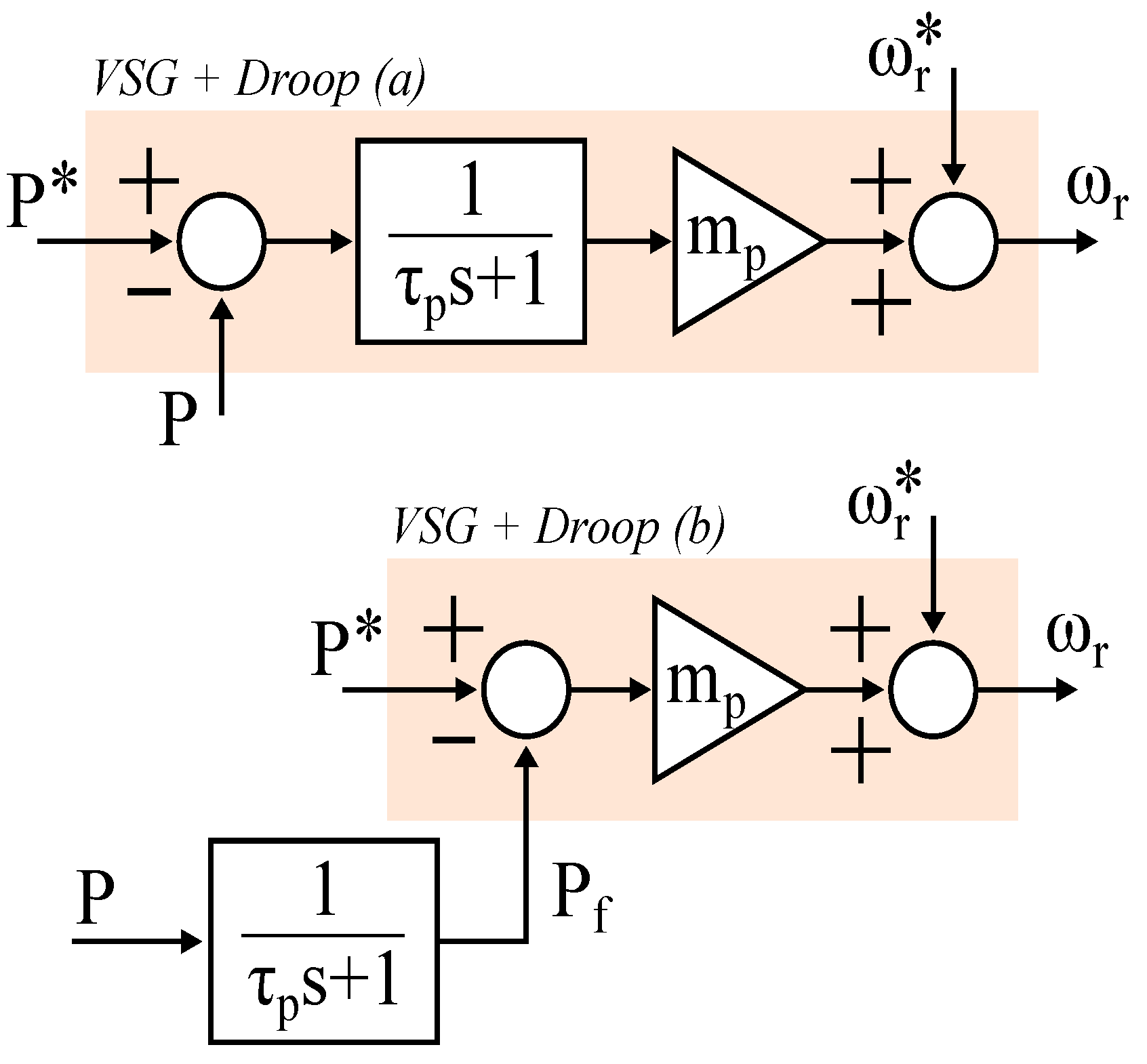
The most common PSL structures in GFM are the Virtual Synchronous Generator (VSG) and the droop-based VSG. By applying these control structures to the generalized small-signal form, the small-signal model can be represented as shown in Figure 3. Although the formulations may differ, they are mathematically equivalent (3).

$${\displaystyle \frac{\Delta {\omega }_r}{\Delta P}}=-{\displaystyle \frac{m_p}{{\tau }_{p}s+1}}={\displaystyle \frac{1}{({\tau }_p/m_p)s+1/m_p}}$$

(3)

In short, the system presented in Figure 2 includes one controlled input $\Delta P^{*}$ and one perturbation, the grid frequency $\Delta {\omega }_r$. Thus, two transfer functions can be evaluated: the power response of the VSG to power setpoint variations (4) and the power response to grid frequency perturbations (5).

$${\displaystyle \frac{\Delta P}{\Delta P^{*}}}=-{\displaystyle \frac{G_c{\omega }_b{K}_t}{s+G_c{H}_c{\omega }_b{K}_t}}$$

(4)

$${\displaystyle \frac{\Delta P}{\Delta {\omega }_g}}=-{\displaystyle \frac{{\omega }_b{K}_t}{s+G_c{H}_c{\omega }_b{K}_t}}$$

(5)

The first equation describes the dynamics of the active power loop, relevant to analyzing the compatibility and design of any higher-level control algorithm (such as POD-P). The second equation is relevant to analyzing the inherent GFM behaviour, i.e., the inherent contribution of the GFM inverters to the rotor angle stability (damping, inertia, …).

As both PSL controls are equivalent, conclusions are valid for both strategies. In this analysis, the filtered droop case is only considered to prevent equation duplication.

2.1. Network Frequency Perturbation Visualization Method

The state-space modeling and eigenvalue analysis method provides valuable information regarding a system’s damping ratio and natural frequency. However, obtaining the eigenvalues requires complete knowledge of all system parameters. In contrast, the network frequency perturbation (NFP) plot offers significant insights, particularly in scenarios where the plant is treated as a black box, concealing internal details such as control strategies and the precise dynamic behavior of the equipment under study. This makes the NFP plot a valuable tool for system operators. Consequently, its application has been recommended for the compliance testing of grid-forming (GFM) plants [29,30].

The NFP method [31,32,33] involves embedding the device within a hypothetical power system in which the network frequency is deliberately modulated in a sinusoidal manner at a specified frequency. This modulation originates from an upstream “infinite bus” and includes sub-synchronous frequency components ranging from 0 Hz to 20 Hz, with optional extension to frequencies near the fundamental. The resulting graphical representation illustrates the device-level behavior of a grid-connected generation unit during system frequency variations.

The NFP plot can be obtained either by deriving the system’s closed-loop transfer function (see Section 2.2) or by conducting time-domain simulations or experimental tests (see Section 4).

Individual synchronous generators (SGs) or GFM devices are expected to contribute to frequency stability and active power balance in a predictable and well-characterized manner. Therefore, even with the addition of various control subsystems—whether internal loops or supplementary controllers for damping—their dynamic response should closely resemble, or be equivalent to, that of a synchronous machine, as described by Equation (5).

To support this analysis, a specific case based on Equation (5) is illustrated in Figure 4, providing a graphical interpretation of the characteristic regions expected from a GFM or SG unit. Although the base case is presented in the following subsection, the example shown in Figure 4 is generated under identical conditions, with the sole variation being the control parameters, ${\tau }_p$ and $m_p$, which are adjusted to emphasize the resonance effects associated with system inertia. The NFP, represented as a Bode plot, highlights three primary features, along with several subtler aspects that can be further interpreted to improve understanding of the device’s overall performance.

Droop Behavior:

The droop behavior of the device becomes evident as the modulation frequency approaches zero (i.e., steady-state conditions). At this frequency, the magnitude response coincides with the droop coefficient, while the phase response approaches 180°, reflecting the inverse relationship between active power and grid frequency. This behavior predominates in the low-frequency range, typically between 0 Hz and 0.5 Hz, depending on the device’s damping characteristics. The droop behavior can be analytically verified by substituting s = 0 into equation (final value theorem) (5).

Inertia:

The inertial response is prominent in the frequency range from approximately 0.2–0.5 Hz up to 1–3 Hz. It is represented in the plot by the inertia asymptote, depicted as a dashed black line that excludes the effects of droop response, rotor resonance, and damping (see Figure 4). Devices possessing inertia typically exhibit a resonance frequency resulting from their second-order system dynamics. This resonance generally appears between 1 Hz and 3 Hz and is influenced by factors such as the inertia time constant, damping coefficient, and total system reactance.

In power electronic converters designed to emulate inertial behavior, these parameters can be adjusted to tune the resonance characteristics. For example, increasing the damping coefficient (corresponding to lower $m_p$ values) enhances system damping, as evidenced by the phase curve moving closer to 180°. The inertial region can be identified using the inertia asymptote, given by $\Delta P$/$\Delta {\omega }_g$ = ${\tau }_p$/$m_p$= 2H, Equation (3).

High-Frequency damping or synchronizing power:

At higher frequencies, the NFP plot reveals the device’s response to rapid changes in grid frequency or phase-angle disturbances. As the modulation frequency increases, the amplitude response steadily decreases. For ideal synchronous generators (SGs) or synchronous condensers (SCs), the phase response drops and eventually stabilizes around 90° near the fundamental frequency. This phase shift reflects a reduction in the damping power component and an increase in the synchronizing power component. The latter is characterized by active power variations that are in phase with changes in the load angle—corresponding to a 90° phase lead relative to frequency variations. This behavior ensures a positive synchronizing power contribution and contributes to stable dynamic performance.

For devices designed to exhibit grid-forming (GFM) behavior, it is essential to replicate these distinctive SG characteristics. Moreover, any additional control loops must preserve, rather than alter, this inherent dynamic behavior.

2.2. Base Case and Theoretical NFP Results

In order to verify the theoretical background presented in previous subsections, a base case using the system presented in Figure 1 with the parameters listed in

Table 1. Base case parameters.

	Var Name	Value
Inertia 2.5 s	$m_p$	0.005/0.01/0.015 pu
	$t_f$	0.025/0.05/0.075 s
Inertia 5 s	$m_p$	0.0025/0.005/0.0075 pu
	$t_f$	0.025/0.05 /0.075 s
LCL filter	$L_c$	0.1 pu
	$C_f$	0.05 pu
	$L_t$	0.05 pu
Grid	$L_g$	0.1 pu
	$R_g$	0 pu

is considered. For this base case, the NFP plot for different sets of parameters are obtained using the general Equation (5) particularized to Equation (6).

$${\displaystyle \frac{\Delta P}{\Delta {\omega }_g}}=-{\displaystyle \frac{({\tau }_{p}s+1){\omega }_b{K}_t}{{\tau }_p{s}^2+s+m_p{\omega }_b{K}_t}}$$

(6)

In looking into more detail in Figure 2, there is more than one set of parameters to synthesize the same inertia. Thus, to analyze the inherent GFM contribution, various values of $m_p$ for synthesizing the same inertia considering two different cases (H = 2.5 s and H = 5 s) are presented in Figure 5.

As expected, at low frequencies, the droop region is characterized by a response dominated by the droop term $m_p$ with a phase shift around 180°. In the present base case, the droop region goes from 0 to 0.5 Hz approximately. The amount of exact damping provided by each control setting can be seen in this region. The larger the dB-value, the more damping it provides to the grid. As the phase shift remains almost constant. It is also possible to see that the increase in the damping makes it harder to see the inertia resonance. But the value of the gain around the inertia asymptote is similar. In summary, the static gain represented by the active power droop ($m_p$) provides damping at control frequencies, while inertia supplies active power in response to frequency variations within the range of the inertia constant. Thus, depending on the inertia constant and how the inertia is implemented in the GFM control, the same IBR with the same inertia will provide a different damping at low frequencies.

At high frequencies, a gain of −20 dB/decade and a phase shift of 90° can be seen, which ensures proper synchronization power.

2.3. Base Case and Active Power Control Loop

To complete the analysis, the active power dynamics under setpoints is determined by Equation (7), a particularized form of Equation (4). Again, various values of $m_p$ are considered, including two different inertia cases (H = 2.5 s and H = 5 s). Results are shown in Figure 6.

$${\displaystyle \frac{\Delta P}{\Delta P^{*}}}=-{\displaystyle \frac{m_p{\omega }_b{K}_t}{{\tau }_p{s}^2+s+m_p{\omega }_b{K}_t}}$$

(7)

Looking at the results, the control bandwidth is way lower than in GFL (which is typically in the range of 100–200 Hz or higher [34]), and again, it is closely related to the emulated inertia. The larger the inertia, the smaller the bandwidth.

Some control structures in GFM allow for the implementation of the inertia with larger bandwidth for the active power setpoint [35], for example, the scheme depicted in Figure 7 with the transfer function expressed in Equation (8).

$${\displaystyle \frac{\Delta P}{\Delta P^{*}}}=-{\displaystyle \frac{m_p{\omega }_b{K}_t}{s+m_p{H}_c{\omega }_b{K}_t}}$$

(8)

However, this increment in the bandwidth (Figure 8) comes at the cost of a less damped response, and the bandwidth still highly depends on the inertia.

2.4. Summary

In order to increase the damping provided by the GFM-based IBR, there are two possibilities: reduce the droop constant (increasing the emulated inertia or not), which increases the damping, or implement an additional POD control loop.

This second option is more complex—especially when a POD-P structure is used. The general dynamics and properties of the GFM can be significantly altered, potentially reducing the provided inertia or even leading to system instability. Therefore, this option should not be implemented lightly. A thorough analysis of the interaction between the POD-P structure and the specific GFM control is essential. This paper proposes the use of the NFP visual method as a tool for this analysis.

GFM control also supports the implementation of POD-V and POD-Q loops. These two methods use voltage variation to damp low-frequency oscillations (LFOs) but they present some limitations compared to active power-based methods. For instance, the voltage at the point of common coupling (PCC) must remain within certain limits—typically ±10% of the rated voltage—restricting the variation range. As a result, the reactive power output from the POD-Q or POD-V algorithms must be kept within these bounds. Additionally, the effectiveness of reactive power injection depends on the short-circuit ratio (SCR) of the grid: the higher the SCR, the lower the impact of injected reactive power on PCC voltage. In strong grids, this effectiveness can be very limited.

In summary, while POD-V and POD-Q introduce fewer control compatibility issues than POD-P, their damping effectiveness may be reduced under specific conditions. It is important to highlight that the use of POD-Q or POD-V does not exclude the implementation of POD-P [2].

Since POD-P/V algorithms generally present low compatibility issues with GFM control, their structure is very similar to those used in STATCOMs or HVDC inverters. As a result, current research primarily focuses on POD-P controls.

3. POD-P Algorithms for GFM Control

3.1. Classic POD and GFM

The classic POD method is based on the inclusion of an additional high-level control loop, which typically uses the angle difference—or a variable related to it—as the input signal to detect power oscillations. Based on this detection, and after appropriate signal processing, an output reference (voltage, reactive power, or active power) is generated for the lower-level control loops.

As a first approach to implementing a POD-P algorithm in a GFM IBR, the same procedure and control structure as the classic POD is used. The control scheme consists of a washout filter, an optional number of lead-lag compensators, and a gain. The time constant of the washout filter ensures that the POD operates only at low frequencies and removes any DC component from the input signal. Lead-lag compensators, if included, allow for the adjustment of the phase angle at the target frequency. In this initial implementation, however, no lead-lag compensators are used.

To analyze this first case, power oscillations are detected directly from the active power. Since lead-lag compensators are not considered in this first approach, the small-signal model of the system corresponds to the one shown in Figure 9.

Figure 9 builds upon Figure 2, where the feedback transfer function $H_c$ is modified by introducing the classic POD structure (without lead-lag components). The NFP Bode plot of the system is derived using Equation (5), with parameters $K_p=1$ and ${\tau }_w=1.6$ s. The results, shown in Figure 10, compare the base case (GFM without POD, blue line) with the case including the POD (red line). It can be observed that at very low frequencies, the POD does not affect the frequency response due to the presence of the washout filter. Similarly, at high frequencies, both configurations behave almost identically, effectively filtering out perturbations.

However, in the inertia region, although the GFM inverter provides increased damping—i.e., more injected active power for the same frequency variation—there is a significant impact on the phase angle. More critically, the inertia behavior of the GFM inverter is completely altered, and the intrinsic damping of the inverter is degraded (see Figure 10).

When the classic POD is implemented in a GFL structure, the injected active power is independent of frequency variation. The phase-locked loop (PLL) provides a stable reference for low- and medium-low frequency variations, while the active power loop (typically implemented with a PI controller) offers sufficient bandwidth. As a result, the only contribution to frequency-dependent behavior comes from the POD algorithm. These assumptions, however, no longer apply in GFM systems, where the natural response to frequency variations must be preserved.

In the case of the POD-P structure implemented within a GFM, the use of second-order band-pass or band-stop filters is recommended. These filters help mitigate the impact of the POD on the synthesized inertia and damping, confining its effect to a specific frequency band. This approach is analyzed in detail in the following section.

3.2. Proposed POD-P

Based on the results presented in the previous subsection—where the washout filter exhibited a significant influence on the system’s low-frequency response—a simplified POD-P method is proposed for integration into GFM control schemes. The key advantage of this approach lies in its simplicity, delivering the desired damping effect at a narrow frequency band while preserving the response across other frequency components.

A POD structure based on a band-pass filter is proposed. Building upon the control loop depicted in Figure 2, the feedback transfer function $H_c$ is modified by incorporating the aforementioned band-pass filter and an associated gain, as illustrated in Figure 11.

To tune a second-order band-pass filter, the target frequency (band-pass center frequency, ${\omega }_n$) and the quality factor (Q = 1/2$\zeta$) have to be adjusted. The center frequency determines the frequency at which the filter has the maximum gain. Thus, if an oscillation is detected in the grid, the measured power oscillation frequency would be the target frequency.

The quality factor affects the bandwidth of the filter: a higher Q results in a narrower and sharper peak, while a lower Q broadens the response. In the Bode plot, changing center frequency shifts the peak of the magnitude response along the frequency axis, while modifying Q alters the slope of the roll-off and the sharpness of the peak. Additionally, the phase response is also affected, becoming steeper around the center frequency as Q increases. Proper tuning is essential to ensure that the filter isolates the desired frequency range without excessive distortion or attenuation in the rear. With more localized power oscillation, higher Q factors can be used. However, it is not recommended to surpass the 200° phase shift mark used to limit the droop region (Figure 4).

In this second case study, a natural frequency of ${\omega }_n=0.3·2·\pi$ and a damping ratio of $\zeta =0.1$ are considered. The results are again compared with the base case (i.e., without a POD structure, shown in blue), as depicted in Figure 12.

The proposed POD structure has a very localized effect on the frequency—active power response of the GFM unit. Its influence is confined to a narrow frequency band of interest. Although a minor reduction in damping capability may be observed, the angle shows a dispersion in the rear of the objective frequency. However, larger damping can be achieved with the same droop constant and without modifying system inertia, static gain, and synchronization power.

Several methods can enhance damping in GFM inverters by adjusting the power synchronization loop (PSL). As the power grid evolves due to demand, generation, or operator actions, its characteristics shift over time. In this context, the simplicity of the proposed POD-P method is advantageous, allowing for the easy reconfiguration of the targeted frequency band as the grid changes.

4. Experimental Validation

4.1. Method

The validation of the results was carried out using the NFP method through multiple time-domain tests. Validating the GFM properties as a whole requires the analysis and evaluation of a wide range of operating points. The NFP plot can be used as a tool to identify the characteristic behavior of a GFM inverter system, and thereby distinguish it from other GFM controls or even from GFL systems. Furthermore, the NFP Bode-like plot provides a visual way to observe the GFM characteristics at a glance and synthesize dozens of simulation results into a single graph [32,33].

The objective of this work is not only to demonstrate that a POD algorithm can be implemented in GFM control and tested in a working case. The main goal is to prove that the theoretical analysis and constraints described in the previous sections are valid. To this end, instead of testing a single case, the GFM inverter control algorithm was modified and evaluated for the different configurations presented. NFP Bode plots were obtained for each parameter set.

First, Bode plots were generated for different values of $m_p$, synthesizing the same inertia (H = 2.5 s and H = 5 s), for both the $\Delta P/\Delta {\omega }_g$ and $\Delta P/\Delta P^{*}$ cases. The former is obtained by exciting the system frequency with a sinusoidal signal, and the latter by exciting the active power setpoint of the inverter. In both cases, the output active power of the inverter was recorded.

The Bode plots were validated by obtaining the same frequency response on both the test bench and the theoretical model. The amplitude of the excitation signal was compared to the output signal, and their ratio in [dB] was used to draw the magnitude of the Bode plot. Regarding phase, the phase shift between the excitation and output signals was calculated from the measurements. For each Bode plot, 16 operating points were measured—that is, 16 different excitation frequencies were applied, and the system’s response was recorded. After validating the base cases, the proposed POD-P control was also validated using the same procedure.

4.2. Experimental Setup

The setup consisted of three main parts: the GFM inverter, the connection filter and impedance, and a controlled voltage source capable of emulating the grid. A photo of the setup with the real components is shown in Figure 13a, and the main diagram in Figure 13b.

The GFM IBR consists of two inverters connected in a back-to-back topology. One of them emulates a battery, with the sole purpose of generating a stiff 320 Vdc bus. The second inverter operates as a three-phase inverter used to test different SVG strategies. Both inverters are commercial INF-50 power inverters from Dutt Electronics. The grid was emulated using a 320-AMX bidirectional three-phase power supply from Pacific Power, which is capable of generating sinusoidal perturbations in order to obtain the $\Delta P/\Delta {\omega }_g$ response of the GFM inverter. The inverter under test and the grid were coupled using an LC filter with damping resistors in series with the capacitor. An additional RL branch was used to emulate the grid impedance. All passive elements and sensing devices were off-the-shelf components.

An OP4512 from OPAL-RT, which includes a Quad-Core 3.7 GHz CPU and a Kintex-7 FPGA, was used as the control hardware. Control algorithms, signal acquisition, and grid voltage management were centralized in this control device.

The main parameters of the setup are summarized in

Table 2. Experimental setup parameterss.

	Var Name	Value
Base values	$S_b$	625 W
	$v_b$	200 V
	${\omega }_b$	314 rad/s
LCL filter	$L_c$	0.1 pu
	$R_c$	0.006 pu
	$C_f$	0.05 pu
	$R_f$	0.08 pu
	$L_t$	0.05 pu
Inverter	$f_{sw}$	10 kHz
	$v_{dc}$	300 Vdc
PSL and RPC setpoints	$P^{*}$	0 pu
	${\omega }_r^{*}$	1 pu
	E	1 pu
Grid	$v_g$	1 pu
	${\omega }_g$	1 pu
	$L_g$	0.1 pu
	$R_g$	0 pu

.

4.3. Experimental Results

The Bode plots obtained analytically were validated using the experimental setup shown in Figure 13, following the method described in the previous section. In Figure 14, the analytical $\Delta P$/$\Delta {\omega }_g$ NFP Bode plots are shown, with the measured points overlapping on the curves. For the three curves, each measured dot shares the same color as its corresponding analytical line. A total of 16 measurements were performed for each case, extracting one point for the magnitude and another for the phase from each measurement—96 measurements in total.

All measured points exhibit a clear trend, validating the analytical expressions developed for the basic case. The largest deviations appear at the highest frequencies, where measurement perturbations and errors become more prominent, particularly around 90° of phase shift. Nonetheless, these discrepancies remain within acceptable limits.

In Figure 15, the analytical $\Delta P$–$\Delta P^{*}$ Bode plots are shown, again with the corresponding measured points overlapping. As in the previous case, 16 measurements were taken for each configuration, resulting in another set of 96 points. The experimental results show a consistent trend that aligns with the theoretical curves.

In addition to the base case Bode plot, this work also evaluated the potential of increasing the control bandwidth of the active power setpoint, as well as the inclusion of the classic POD control structure and the proposed POD-P structure. The Bode plots and analytical transfer functions for these three cases are shown in earlier figures. However, the validation of the first two alternatives was excluded. Increasing the bandwidth through alternative techniques complicates the POD-P algorithm and interferes with the inherent control of the GFM system. For the second case, adding the classic POD structure not only alters the GFM control characteristics but could also compromise the stability of the inverter. Therefore, the focus of this study is on the validation of the transfer function and Bode plot corresponding to the proposed POD-P algorithm. Validating non-relevant cases would not contribute meaningful information to the reader, and the validation of an unstable control design may not be feasible.

In Figure 16, the analytical $\Delta P$/$\Delta {\omega }_g$ NFP Bode plot of the proposed POD-P control and its equivalent base case are shown. The measured points can be seen overlapping. In total, 11 additional measures were taken at low frequencies to obtain a better accuracy at those frequencies. The measured operation points correspond almost perfectly to the theoretical results. The Bode plot of the proposed POD-P algorithm shows that a POD-P structure can work properly in a GFM-based IBR, without interacting negatively with each other.

The inherent GFM characteristics are not modified, while the provided damping at the selected frequency increases. However, it is important to highlight that at the corners of the band, a little damping capacity can be lost.

5. Discussion

From the different ways to provide damping to LFOs using a GFM inverter, those based on reactive power are not specially affected by the change in the control paradigm from GFL to GFM.

This paper, therefore, focuses on active-power-based damping strategies, presenting the analytical and theoretical background for both the inherent damping capability of GFM control and the role of active power setpoint dynamics. By appropriately tuning the inertia and droop parameters, GFM inverters can effectively provide damping. Inertia is synthesized using two parameters ($m_p$ and ${\tau }_f$), and the proper selection of these can be sufficient for most applications. However, this technique has inherent limitations: increasing damping performance often results in heightened sensitivity of the GFM control to frequency perturbations. Nonetheless, if system conditions allow for the use of a reduced droop coefficient, this method remains the simplest, most robust, and effective option.

When tuning droop parameters alone does not achieve sufficient damping, a higher-level POD-P algorithm can be implemented. So, in recent years, many POD-P solutions have appeared for GFM-controlled inverters. However, few of these approaches evaluate the influence of the POD-P control structure on inherent GFM functionalities, such as inertia, damping, or synchronizing power. Given the potential of POD-P algorithms to significantly alter these characteristics, it is essential to assess and verify the behavior of GFM systems when such controllers are introduced.

Unlike GFM inverters, GFL-controlled inverters do not possess intrinsic dynamic characteristics, as they merely follow current setpoints. Consequently, in GFL systems, the application of POD-P control does not alter the device’s nature. In contrast, with GFM inverters, integrating a POD-P controller requires a revised methodology to ensure core dynamic properties remain unaffected. This study addresses these concerns by analyzing the impact of the POD-P structure on GFM behavior using a NPF method.

The NFP method, based on perturbations generated by an infinite bus, does not take into account grid details, so the verification is not grid-oriented. However, from the perspective of system operators (or inverter manufacturers who must comply with grid codes), the NFP method is very interesting as it guarantees GFM core functionalities for specific equipment.

Several techniques exist to improve damping in GFM inverters by adapting the PSL. While many of these strategies are either tailored to specific grid configurations or provide general tuning frameworks, the reality is that the power grid is a dynamic and evolving system. Changes in demand, generation, or operator actions can alter grid characteristics over time. In this context, the simplicity of the proposed POD-P method becomes an advantage. Its simplicity allows us to reconfigure the targeted frequency band, offering a form of user-supervised adaptability.

Taking all the above into consideration, and recognizing that droop tuning remains the most straightforward and preferred method for providing damping, the proposed POD-P algorithm demonstrates that additional damping can be introduced into GFM-based inverter-based resources (IBRs) without compromising their inherent capabilities. Furthermore, the control strategy can be easily configured without requiring prior knowledge of grid parameters.

6. Conclusions

The analytical and theoretical results were validated in a testbed. Over 200 measurements were taken and analyzed, all of which were consistent with the analytical equations. The measured operating points closely overlapped with the theoretical Bode plots in both magnitude and phase, validating both the analytical model and the effectiveness of the POD-P algorithm in grid-forming inverter-based resources (GFM IBRs). The algorithm operates within a narrow frequency band in the droop region, ensuring that the inherent capabilities of the GFM system are maintained.

The optimal and most recommended approach for providing additional damping is tuning the grid-forming parameters, as this is significantly simpler. If this approach is not feasible or does not provide sufficient damping, a POD-P algorithm can be employed. However, in such cases, it is essential to validate the preservation of grid-forming properties.