Rate of Penetration Estimation with Parameter Correction

Abstract

Accurate estimation of the Rate of Penetration (ROP) is essential for optimizing drilling operations, particularly in deep wells where traditional methods based on nominal depth measurements often fall short. These conventional approaches typically overlook dynamic influences such as drill string elongation caused by tension, hydraulic pressure, and thermal effects, leading to significant errors in ROP estimation. This study introduces a comprehensive method that integrates well depth correction and dynamic modeling of drill string elongation to enhance ROP accuracy. Furthermore, model-based filtering techniques are incorporated into a dynamic ROP estimation framework to improve real-time performance. Simulation results indicate that the combination of elongation corrections and filtering significantly reduces estimation errors and enhances reliability under varying drilling conditions. The proposed method provides a more accurate and robust ROP estimation framework, contributing to improved real-time monitoring and operational decision-making in drilling processes.

1. Introduction

1.1. Depth Corrections

Well depth measurement is a fundamental aspect of drilling operations in the Oil and Gas industry, serving as a crucial parameter for a variety of operational decisions, including the estimation of the Rate of Penetration (ROP), wellbore positioning, and drilling efficiency optimization. The accuracy of well depth measurements is critical because errors in these measurements can lead to significant operational inefficiencies, increased costs, and safety risks. However, achieving precise well depth measurement is challenging due to various factors, such as the physical properties of the drill string, dynamic drilling conditions, and inherent limitations of measurement techniques. To address these challenges, numerous studies have focused on measured depth correction methods, as discussed in [1,2,3,4].

Traditionally, well depth is estimated by measuring the length of the drill string deployed into the wellbore, assuming that this length corresponds directly to the depth of the well. However, this approach does not account for several dynamic factors that can affect the actual depth, such as drill string elongation due to tension, compression, thermal expansion, and pressure effects. Moreover, the dynamic nature of drilling operations, including changes in weight on bit (WOB), rotational speed, and fluid dynamics, further complicates the accurate measurement of well depth. These factors can cause the drill string to stretch, contract, or bend, leading to deviations from the true well depth.

One of the primary sources of error in well depth measurement is the elongation of the drill string due to tension. As the weight of the drill string increases with depth, it causes the string to stretch, leading to an overestimation of the well depth. In [5], the authors emphasized the importance of accounting for tension elongation in well depth measurement and proposed a correction model that incorporates drill string compliance. Their work demonstrated that neglecting tension elongation could result in significant depth measurement errors, particularly in deep wells. Moreover, hydraulic effects, including pressure ballooning and flow-induced lift, can also cause errors in well depth measurement. In [6], these hydraulic effects are explored and correction models are developed to account for them, showing that these factors become increasingly significant in high-pressure environments. In addition, thermal expansion of the drill string, caused by temperature variations along the wellbore, is another factor that can lead to inaccuracies in well depth measurement. As the drill string is exposed to higher temperatures at greater depths, it expands, causing an overestimation of the well depth.

Another critical factor influencing well depth measurement is the correction of WOB, which significantly affects the accuracy of depth estimation, particularly in deep wells. WOB directly impacts the force exerted at the bit, influencing both ROP and wellbore stability [7]. However, inconsistencies in WOB measurements can introduce errors in depth calculations due to drill string deflection, dynamic interactions with the wellbore, and unaccounted physical forces acting along the drill string. One approach to improving WOB accuracy involves compensating for the discrepancies between surface-derived WOB and true downhole conditions. For example, in [8], the authors analyze the limitations of deriving WOB and Torque on Bit (TOB) from surface measurements, emphasizing the impact of unmodeled physical processes occurring between the bit and surface equipment. To address these discrepancies, they propose real-time compensation methods based on torque, drag, and hydraulic calculations, which refine WOB estimations and ultimately enhance drilling efficiency and bit performance. Another crucial refinement to WOB correction focuses on the accuracy of reference hook load measurements. In [6], the authors challenge the assumption that reference hook load remains constant by identifying and analyzing seven key factors affecting it: wellbore friction, added weight in air, well inclination, flow-induced lift, nozzle jet lift, cuttings in suspension, and back pressure in managed pressure drilling operations. By integrating these factors into correction models, they develop a systematic approach to improve WOB accuracy and minimize errors arising from fluctuating hook load values. A more direct method for WOB correction is the use of downhole measurement techniques to obtain real-time force readings at the bit. In [9], the authors propose a Downhole WOB measurement approach based on the force–strain principle, addressing the shortcomings of surface-based WOB estimations. Their method models the linear relationship between axial force, fluid pressure, and temperature difference while incorporating the effects of nozzle jet force, flow friction force, and lift force. This refined DWOB equation is validated through finite element simulations and field experiments, achieving measurement errors within ±1000 N and ±5000 N, respectively. The study highlights the benefits of DWOB correction in improving bit life and increasing ROP, demonstrating the significance of integrating real-time downhole measurements into WOB estimation frameworks.Additionally, various other studies have explored different WOB correction approaches, including advanced modeling techniques and real-time measurement strategies, see, for example [10,11].

1.2. ROP Estimation

The ROP is a critical parameter in drilling operations, directly influencing the efficiency, cost, and safety of wellbore construction. The ROP represents the speed at which the drill bit advances through the formation, and it is a key indicator of drilling performance. Accurate ROP measurement is essential for optimizing drilling parameters, such as WOB, RPM, and mud properties to achieve the desired drilling outcomes while minimizing operational costs, see works on ROP optimization [12,13,14]. However, calculating the ROP accurately is challenging due to the complex interplay of various factors, including well depth, formation properties, and dynamic drilling conditions. Traditionally, the ROP is calculated by dividing the depth increment drilled over a specific time interval by the time taken to drill that increment. This method, while straightforward, can lead to inaccuracies due to several factors that are often overlooked, such as drill string elongation, wellbore trajectory, and real-time variations in drilling parameters. Moreover, as drilling progresses to greater depths, the physical and dynamic conditions of the wellbore change, further complicating the accurate calculation of ROP.

The relationship between well depth and the ROP is fundamental to drilling operations. In [5], it is highlighted that well depth directly influences ROP, as the depth measurement is integral to calculating penetration rates. Their research emphasized the need for accurate depth correction to avoid significant errors in ROP estimation, particularly in deep wells where elongation effects become more pronounced. In [6], correction models are presented to account for many factors, like drill string elongation, dynamic conditions, and thermal expansion to enhance accuracy. In [15], the authors provided a comprehensive survey of filtering techniques, including their applications to depth measurement in drilling operations. Their work highlights the importance of these techniques in improving the accuracy of depth measurements in complex drilling environments.

1.3. Motivation, Novelty, and Contribution

The motivation for this study stems from the pressing need to improve the accuracy of well depth (measured depth) and ROP estimation, especially in the context of modern, deep, and complex wellbores. Traditional methods typically assume that the nominal drill string length corresponds directly to the true well depth and that ROP can be derived by simply differentiating depth over time. However, these approaches often neglect the effects of drill string deformation, sensor uncertainty, and dynamic downhole interactions—leading to significant errors, suboptimal parameter tuning, and increased operational risk. The novelty of this work lies in a comprehensive and physics-informed methodology that integrates advanced well-depth correction models with a Kalman filter-based real-time estimation framework. Specifically, our method introduces two key innovations over conventional approaches:

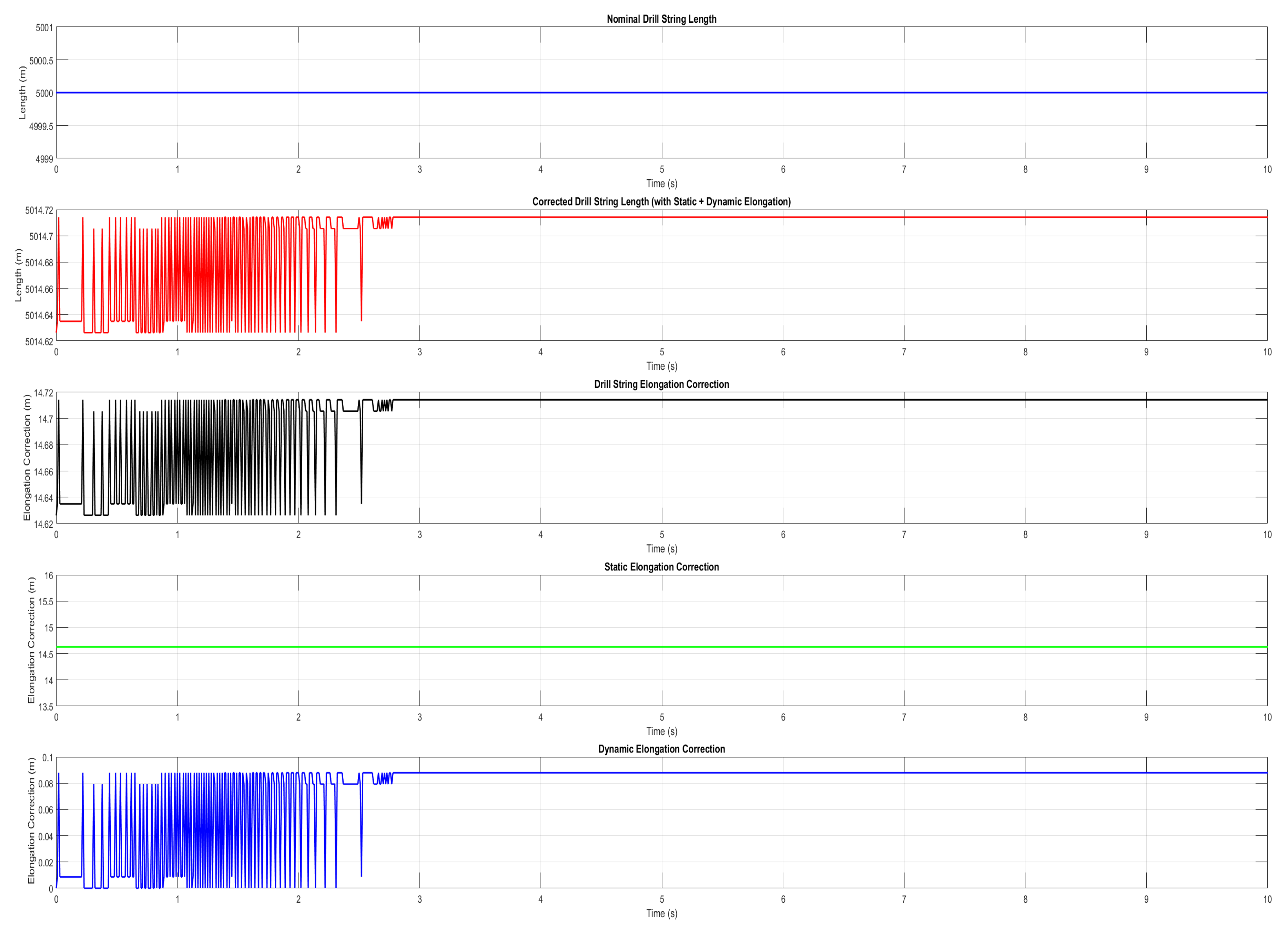
• Integration of static and dynamic elongation: The proposed model separates and accounts for both static elongation (due to tension, pressure ballooning, thermal expansion, and friction drag) and dynamic elongation (induced by vibration, bit–rock interaction, and transient axial loads). This dual-component correction enables a more accurate determination of the bit’s true position in the formation—critical for high-resolution control and monitoring in deviated or deep wells.
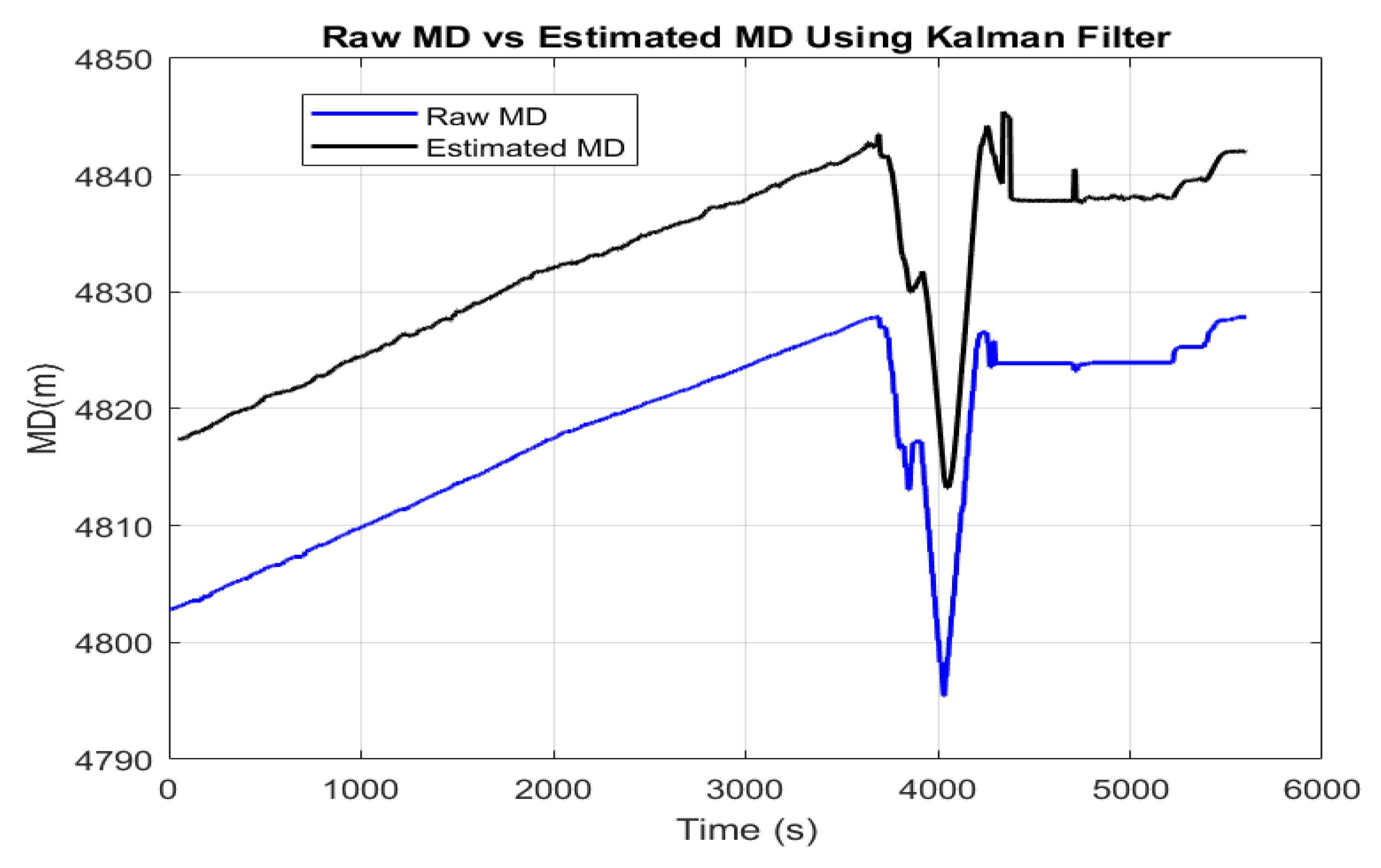
• Kalman filter-based ROP estimation: A state-space model incorporating ROP, bit penetration, and dynamic elongation is formulated, and a Kalman filter is employed to iteratively estimate these variables in real time. This method not only filters out sensor noise and measurement drift but also improves robustness against modeling uncertainties, providing smoother and more reliable ROP estimates than traditional time-differentiation methods.

By combining dynamic modeling and real-time filtering, the proposed framework offers a significantly improved solution for accurate depth tracking and ROP calculation. These improvements have direct implications for enhanced drilling automation, real-time decision-making, and safe, cost-efficient operations.

2. Well Depth Correction

2.1. Downhole Forces

WOB is a crucial parameter in drilling operations, directly influencing the ROP and the mechanical energy applied to the formation. However, the measured WOB at the surface does not always accurately represent the true downhole WOB due to factors such as frictional drag, axial elongation of the drill string, and hydraulic forces acting on the system [11,16]. One of the primary sources of error in surface WOB measurement arises from frictional drag between the drill string and the wellbore. As the drill string moves along the well trajectory, contact with the wellbore wall generates axial friction forces that reduce the effective force transmitted to the bit. This effect becomes particularly pronounced in deviated and horizontal wells, where the lateral contact between the drill string and wellbore significantly increases frictional resistance. The frictional loss can be modeled using the following equation:

$$F_{friction}={\mu }_a·F_c,$$

(1)

where ${\mu }_a$ is the axial friction coefficient, and $F_c$ is the normal contact force along the wellbore, which is a key parameter affecting frictional losses along the wellbore. In [17], they present the Torque and Drag model that gives the detailed modeling of downhole forces, where $F_c$ is given as

$$F_c=\sqrt{{(wsin\theta -{\mu }_{a}F{\theta }^{\prime })}^2+{({\mu }_{a}Fsin\theta {\phi }^{\prime })}^2}.$$

(2)

Here w is the buoyant weight per unit length, $\theta$ is the inclination, F is the total tension in the string, $\phi$ is the azimuth angle, and ′ denotes differentiation with respect to the measured depth. The axial force along the drill string, F, includes contributions from the axial tension $F_t$ and hydraulic forces acting on the string. It is calculated as

$$F=-WOB+F_t+F_{\mathrm{hydraulic}},$$

(3)

where the axial tension $F_t$ is given by

$$F_t=F_r+F_{friction},$$

(4)

and $F_r$ is the tension at the top as

$$F_r={\int }_0^{L}wcos\theta ds,$$

(5)

and the hydraulic force component is given by

$$F_{\mathrm{hydraulic}}={\int }_0^L(-A_o{p}_q^{\prime }-\pi d_0{\tau }_0)ds,$$

(6)

where $p_q^{\prime }$ is the flow and motion-induced pressure gradient, ${\tau }_0$ is the flow-induced axial shear stress at the outer string surface, and $A_o$ is the respective cross-sectional areas. In the field, the WOB can be estimated from surface measurements using load cells installed on the top drive or hook. The measured WOB is derived from the hook load ($F_h$), accounting for the effects of the submerged weight of the drill string and frictional resistance in the wellbore.

To accurately estimate the WOB and subsequently determine the axial tension force ($F_t$) and hydraulic force ($F_{\mathrm{hydraulic}}$), an iterative correction algorithm based on measured hook load ($F_h$) is employed in this study. This approach ensures consistency between the measured and calculated forces, improving the reliability of the drilling force estimations.

The algorithm begins by setting an initial estimate for WOB, denoted as $WO{B}_0$. This initial guess is used in Equation (3) to compute the axial force F under the given wellbore and operational conditions. Once F is determined, the computed hook load $F_{h,\mathrm{calc}}$ is obtained using the following relationship:

$$F_{h,\mathrm{calc}}=F.$$

(7)

The calculated hook load is then compared with the measured hook load ($F_h$). The difference between these values is defined as the following error:

$$\Delta F_h=F_{h,\mathrm{calc}}-F_h.$$

(8)

The magnitude and sign of $\Delta F_h$ determine whether a correction to WOB is necessary:

• If $\Delta F_h>0$, meaning the calculated hook load is greater than the measured value, the algorithm increases WOB by a predetermined step size to reduce the error.
• If $\Delta F_h<0$, meaning the calculated hook load is lower than the measured value, WOB is decreased to bring the computed values closer to the measured ones.

A correction step is applied iteratively, updating WOB as follows:

$$WO{B}_{n+1}=WO{B}_n-\alpha \Delta F_h,$$

(9)

where $\alpha$ is a tuning parameter that controls the step size of the correction. This process is repeated until $|\Delta F_h|$ is within a predefined threshold, ensuring that the calculated hook load sufficiently matches the measured value. Each update to WOB propagates through the force balance equations, leading to updated values of axial tension force $F_t$ and hydraulic force $F_{\mathrm{hydraulic}}$. The iteration continues until the following convergence condition is met:

$$|\Delta F_h|\le ϵ,$$

(10)

where $ϵ$ is a predefined threshold value ensuring numerical stability. Once the algorithm converges, the final corrected WOB is obtained, along with the updated values for $F_t$ and $F_{\mathrm{hydraulic}}$. This iterative approach improves the accuracy of WOB estimation by systematically refining the value until the calculated hook load aligns with the measured hook load. Figure 1 presents the flow process used for the calculation of the WOB for given data points. The inputs besides the aforementioned are the friction factor, well trajectory, BHA configuration, and fluid density. By incorporating these corrections, the measured WOB provides a more accurate estimate of the actual force applied by the bit to the formation.

2.2. Static Elongation

Traditional methods of measuring well depth typically involve using the nominal length of the drill string as a proxy for true depth. However, this approach overlooks several important dynamic factors that can lead to significant errors, particularly in deep wells. These factors include tension elongation, hydraulic effects, thermal expansion, and dynamic drilling conditions, all of which must be accurately accounted for to improve the reliability of depth measurements. In [6], some of critical elongations are listed, see the details below.

As the drill string is subjected to axial forces due to its weight and the WOB, it experiences tension elongation. The corresponding elongation due to tension can be expressed as

$$\Delta L_{\mathrm{tension}}={\int }_0^L{\displaystyle \frac{F_r\left(s\right)}{E·A\left(s\right)}}ds,$$

(11)

where E is the Young’s modulus of the material and $A\left(s\right)$ is the cross-sectional area of the drill string. When the drill string moves along the wellbore, frictional forces come into play, which affect the tension distribution and elongation. The drag-induced elongation can be approximated by

$$\Delta L_{\mathrm{drag}}={\int }_0^L{\displaystyle \frac{{\mu }_a·F_c\left(s\right)}{E·A\left(s\right)}}ds,$$

(12)

where ${\mu }_a$ is the axial friction coefficient and $F_c\left(s\right)$ is the total normal contact force along the string. The drill string is also subject to hydraulic effects due to the pressures exerted by drilling fluids inside and outside the string. These effects can be significant, especially in high-pressure environments. The elongation due to pressure ballooning is given by

$$\Delta L_{\mathrm{ballooning}}={\int }_0^L{\displaystyle \frac{F_{\mathrm{hydraulic}}}{E·A\left(s\right)}}ds.$$

(13)

The temperature variations along the wellbore cause the drill string to expand or contract, impacting the well depth measurement. The correction for thermal expansion can be written as

$$\Delta L_{\mathrm{thermal}}=\beta ·L·\Delta T,$$

(14)

where $\beta$ is the linear thermal expansion coefficient of the drill string material and $\Delta T$ is the temperature difference along the string. The combined effects of tension, friction, hydraulic forces, and thermal expansion must be considered to accurately correct the well depth. The total elongation of the drill string is given by

$$\Delta L_{static}=\Delta L_{\mathrm{tension}}+\Delta L_{\mathrm{drag}}+\Delta L_{\mathrm{ballooning}}+\Delta L_{\mathrm{thermal}}.$$

(15)

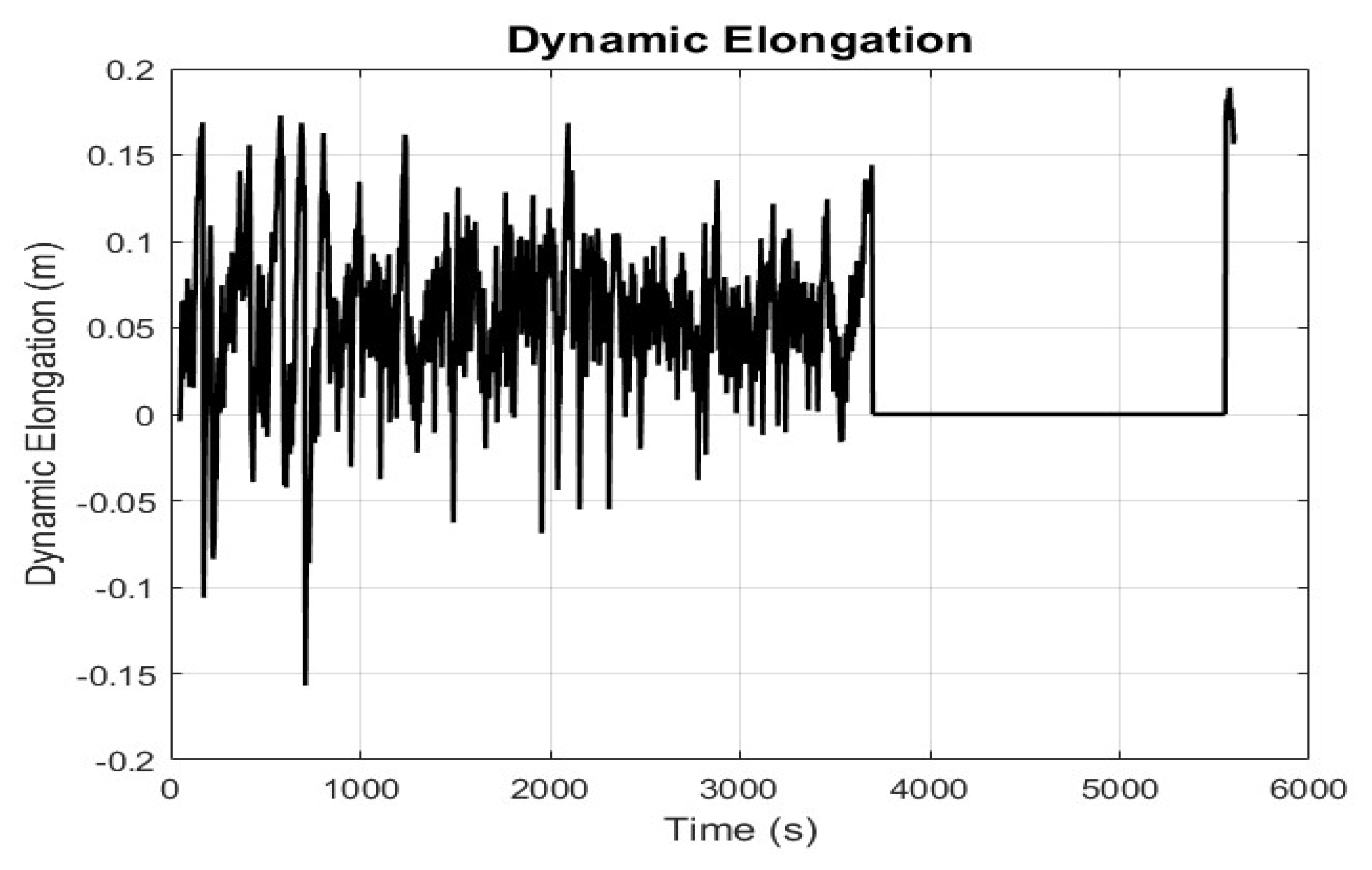
2.3. Dynamic Elongation

Studying dynamic elongation ($\Delta L_{dynamic}$) is crucial because it provides insight into the time-varying deformations of the drill string that directly impact the accuracy of depth measurement and drilling performance.

2.3.1. Drill String Dynamic Model

The drill string dynamic model considers both axial and torsional dynamics of the drill string, which are coupled through the interaction between the drill bit and the formation. The axial and torsional dynamic model from [18] is expressed below:

$$M\ddot{z}\left(t\right)+C_a\dot{z}\left(t\right)+K_a\left(z\left(t\right)-V_{0}t\right)=W_s-W\left(t\right)$$

(16)

where M is the equivalent translation inertia, $C_a$ is the axial damping coefficient, $K_a$ is the axial stiffness, $z\left(t\right)$ is the axial displacement, $V_0$ is the constant axial speed, $W_s$ is the submerged weight of the drill string, and $W\left(t\right)$ is the dynamic force due to bit–rock interactions. For torsional dynamics, the model is formulated as

$$I\ddot{\varphi }\left(t\right)+C_t\dot{\varphi }\left(t\right)+K_t\left(\varphi \left(t\right)-{\mathrm{\Omega }}_{0}t\right)=-T\left(t\right)$$

(17)

where I is the rotary inertia, $C_t$ is the torsional damping coefficient, $K_t$ is the torsional stiffness, $\varphi \left(t\right)$ is the angular displacement, ${\mathrm{\Omega }}_0$ is the constant rotational speed, and $T\left(t\right)$ is the Torque on Bit. The dynamic force $W\left(t\right)$ acting on the drill string is the sum of the cutting force ($W_c\left(t\right)$) and the frictional force ($W_f\left(t\right)$), or

$$W\left(t\right)=W_c\left(t\right)+W_f\left(t\right).$$

(18)

Both of them vary with time due to the changing position and motion of the drill bit. For $W_c\left(t\right)$, it is cutting force, which can be calculated by

$$W_c\left(t\right)=ϵa\zeta R\left(d\left(t\right)\right)H\left(\dot{\varphi }\left(t\right)\right)$$

(19)

where $ϵ$ is the intrinsic specific energy of the rock, a is the radius of the drill bit, $\zeta$ is the cutter face inclination, $R\left(d\right(t\left)\right)$ is the ramp function describing the cutting depth, and $H\left(\dot{\varphi }\left(t\right)\right)$ is the Heaviside function representing the direction of rotation. For the friction force $W_f\left(t\right)$, it can be estimated by

$$W_f\left(t\right)=\sigma alH\left(d\left(t\right)\right)H\left(\dot{z}\left(t\right)\right)$$

(20)

where $\sigma$ is the contact strength, l is the wearflat length of the drill bit, and $H\left(d\right(t\left)\right)$ and $H\left(\dot{z}\left(t\right)\right)$ are Heaviside functions representing the cutting depth and axial motion, respectively. $d\left(t\right)$ is the instantaneous cutting depth as

$$d\left(t\right)=z\left(t\right)-z(t-\tau (t\left)\right)$$

(21)

where $\tau \left(t\right)$ is the state-dependent delay representing the time it takes for the drill bit to rotate and re-engage with the formation.

2.3.2. Dynamic Elongation Calculation

The dynamic elongation $\Delta L_{dynamic}$ can be calculated by

$$\Delta L_{\mathrm{dynamic}}\left(t\right)={\int }_0^L{\displaystyle \frac{W\left(t\right)}{E·A}}ds,$$

(22)

where $W\left(t\right)$ is the dynamic force calculated from the cutting and frictional components, see Equation (18). From the above-mentioned drill string dynamic model, it can be further shown as

$$W\left(t\right)=ϵa\zeta R\left(d\left(t\right)\right)H\left(\dot{\varphi }\left(t\right)\right)+\sigma alH\left(d\left(t\right)\right)H\left(\dot{z}\left(t\right)\right)$$

(23)

It is important to clarify that $\Delta L_{\mathrm{dynamic}}\left(t\right)$ is computed based solely on the time-varying perturbations in axial force—namely, the dynamic deviations from the equilibrium load—caused by drill string vibrations and bit–rock interactions. These fluctuations are superimposed on the nominal static force, which is already captured through the analytical expression for $\Delta L_{\mathrm{static}}$ in Equation (11). To avoid redundancy, the dynamic elongation term is explicitly formulated to exclude static tension effects. In the implementation of Equation (22), the dynamic force $W\left(t\right)$ is defined as the fluctuating component relative to the nominal axial load. This formulation ensures that the mean elongation due to static axial stress is not reintroduced into the dynamic elongation integral. As such, $\Delta L_{\mathrm{static}}$ and $\Delta L_{\mathrm{dynamic}}\left(t\right)$ are treated as complementary and nonoverlapping contributions to the total drill string elongation.

2.4. Well Depth Calculation

The total elongation $\Delta L\left(t\right)$ of the drill string is the sum of the static elongation ($\Delta L_{\mathrm{static}}$) and the dynamic elongation ($\Delta L_{\mathrm{dynamic}}\left(t\right)$) as

$$\Delta L\left(t\right)=\Delta L_{\mathrm{static}}\left(t\right)+\Delta L_{\mathrm{dynamic}}\left(t\right),$$

(24)

where $\Delta L_{\mathrm{static}}$ captures the time-invariant baseline elongation due to steady-state stressors, such as tension, thermal expansion, frictional drag, and hydraulic pressure, and $\Delta L_{\mathrm{dynamic}}\left(t\right)$ represents the time-varying deformation induced by transient forces from drill string vibration and bit–rock interaction. To prevent redundancy, the dynamic model uses only the fluctuating force $W\left(t\right)$ (see Equation (18)), assuming the static baseline is already included in $\Delta L_{\mathrm{static}}$. The well depth (MD(t)), therefore, can be corrected as

$$MD\left(t\right)=M{D}_{measured}\left(t\right)+\Delta L\left(t\right),$$

(25)

where $M{D}_{measured}$ accounts for the height of the top of the string above the drill bit position and the nominal length of the drill string.

3. ROP Calculation

The measured depth is an important quantity in drilling operations, as it represents the total depth along the wellbore from the surface to the drill bit. In addition, the true bit penetration ($\Delta z_{\mathrm{bit}}\left(t\right)$), dynamic elongation, and static elongation of the drill string also play crucial roles in determining the actual progress of the drill bit into the formation. The relationships among these quantities are given below.

$$\mathrm{MD}\left(t\right)={\mathrm{MD}}_{initial}+\Delta z_{\mathrm{bit}}\left(t\right),$$

(26)

where ${\mathrm{MD}}_{initial}$ refers to the initial measured depth at a specific reference point in time during operations. The ROP in drilling operations is determined by measuring the velocity at which a drill bit progresses through the rock or formation being drilled. It is commonly measured in units of depth per unit of time, or

$$\mathrm{ROP}\left(t\right)={\displaystyle \frac{d}{dt}}\left(MD\left(t\right)\right).$$

(27)

In fact, the calculation of the ROP shall consider the time derivative of the true bit penetration ($\Delta z_{\mathrm{bit}}\left(t\right)$) as

$$\mathrm{ROP}\left(t\right)={\displaystyle \frac{d}{dt}}\left(\Delta z_{\mathrm{bit}}\left(t\right)\right).$$

(28)

From Equation (25), it is easy to have

$$\Delta z_{bit}\left(t\right)=M{D}_{measured}+\Delta L\left(t\right)-M{D}_{initial}$$

Rearranging the equation, we have

$$\mathrm{ROP}\left(t\right)={\displaystyle \frac{d}{dt}}\left({\mathrm{MD}}_{measured}\left(t\right)\right)+{\displaystyle \frac{d}{dt}}\left(\Delta L_{static}\left(t\right)\right)+{\displaystyle \frac{d}{dt}}\left(\Delta L_{dynamic}\left(t\right)\right).$$

(29)

The depth interval ${\displaystyle \frac{d}{dt}}\left({\mathrm{MD}}_{measured}\left(t\right)\right)$ can be affected by sensor noise, which introduces random fluctuations in the readings and other errors such as inaccuracies due to drill string elongation or calibration drift. These factors can further cause deviations in the measured depth from the true depth, leading to potential errors in calculating the actual drilling progress. In the next section, the model-based filter is implemented to enhance the ROP calculation with consideration of sensor errors and elongation factors. While $\Delta L_{static}\left(t\right)$ may change gradually over time due to evolving downhole conditions, its temporal variation is significantly slower than that of $\Delta L_{dynamic}$. Hence, the derivative ${\displaystyle \frac{d}{dt}}\left(\Delta L_{static}\left(t\right)\right)$ possibly can be neglected in Equation (29) to simplify the model without sacrificing estimation accuracy. If needed, $\Delta L_{static}\left(t\right)$ can be periodically updated in a slower outer loop.

4. ROP Estimation with Models

4.1. State-Space Model

Since the dynamics of ROP is difficult to model, here we assume that there is no significant change between $\mathrm{ROP}(t+1)$ and $\mathrm{ROP}\left(t\right)$ in a short time interval $\Delta t$. Equivalently, it can be expressed as

$$\mathrm{ROP}(t+1)=\mathrm{ROP}\left(t\right)+{\xi }_1\left(t\right),$$

(30)

where ${\xi }_1\left(t\right)$ is the parameter to represent the model uncertainty. From Equation (28), the system can be easily rewritten as

$$\Delta z_{\mathrm{bit}}(t+1)=\Delta z_{\mathrm{bit}}\left(t\right)+\mathrm{ROP}\left(t\right)\Delta t+{\xi }_2\left(t\right),$$

(31)

where ${\xi }_2\left(t\right)$ is also introduced as some model uncertainties. The model for the dynamic elongation ($\Delta L_{\mathrm{dynamic}}\left(t\right)$) can be considered as

$$\Delta L_{\mathrm{dynamic}}(t+1)=\Delta L_{\mathrm{dynamic}}\left(t\right)-{\beta }_d\left(t\right)\Delta t+{\xi }_3\left(t\right),$$

(32)

where ${\beta }_d\left(t\right)$ is the time constant which dictates the speed at which the system’s dynamic response decays and ${\xi }_3\left(t\right)$ is the parameter to represent the model uncertainty. However, since ${\beta }_d\left(t\right)$ is also a parameter needed to be estimated, it is assumed that

$${\beta }_d(t+1)={\beta }_d\left(t\right)+{\xi }_4\left(t\right).$$

(33)

Here, let the state vector $\mathbf{x}\left(t\right)$ be given by

$$\mathbf{x}\left(t\right)=\left[\begin{array}{c}\mathrm{ROP}\left(t\right)\\ \Delta z_{\mathrm{bit}}\left(t\right)\\ \Delta L_{\mathrm{dynamic}}\left(t\right)\\ {\beta }_d\left(t\right)\end{array}\right]$$

The state equation becomes

$$\mathbf{x}(t+1)=\mathbf{A}\mathbf{x}\left(t\right)+\mathbf{B}\mathbf{u}\left(t\right)+\xi \left(t\right)$$

where $\mathbf{A}$ is the state transition matrix, $\mathbf{B}$ is the input matrix, $\mathbf{u}\left(t\right)$ represents external inputs (if any), and $\xi \left(t\right)$ represents model uncertainties. The state transition matrix $\mathbf{A}$ is

$$\mathbf{A}=\left[\begin{array}{cccc}1& 0& 0& 0\\ \Delta t& 1& 0& 0\\ 0& 0& 1& -\Delta t\\ 0& 0& 0& 1\end{array}\right].$$

The input matrix $\mathbf{B}$ is

$$\mathbf{B}=\left[\begin{array}{c}0\\ 0\\ 0\\ 0\end{array}\right].$$

Assume that the dynamic elongation is obtained from Equation (22) that can be treated as the measurement. The other available parameter is the MD ($M{D}_{measured}$). Given that

$${\mathrm{MD}}_{measured}=\Delta z_{bit}\left(t\right)-\Delta L\left(t\right)+{\mathrm{MD}}_{initial}.$$

One new parameter could be defined as

$$\widetilde{\mathrm{MD}}\left(t\right)={\mathrm{MD}}_{measured}\left(t\right)-{\mathrm{MD}}_{\mathrm{initial}}+\Delta L_{\mathrm{static}}=\Delta z_{\mathrm{bit}}\left(t\right)-\Delta L_{\mathrm{dynamic}}\left(t\right).$$

It can be used as the other measurement for such a control system. Then, the measurement equation is

$$\mathbf{y}\left(t\right)=\left[\begin{array}{c}\widetilde{\mathrm{MD}}\left(t\right)\\ \Delta L_{\mathrm{dynamic}}\left(t\right)\end{array}\right]=\left[\begin{array}{cccc}0& 1& -1& 0\\ 0& 0& 1& 0\end{array}\right]\mathbf{x}\left(t\right)+\mathbf{v}\left(t\right).$$

It is written in general as

$$\mathbf{y}\left(t\right)=\mathbf{C}\mathbf{x}\left(t\right)+\mathbf{v}\left(t\right)$$

where $\mathbf{C}$ is the measurement matrix and $\mathbf{v}\left(t\right)$ is the measurement noise. The measurement matrix $\mathbf{C}$ is

$$\mathbf{C}=\left[\begin{array}{cccc}0& 1& -1& 0\\ 0& 0& 1& 0\end{array}\right].$$

4.2. Kalman Filter Implementation

The Kalman filter, a powerful recursive algorithm for estimating the state of dynamic systems, has been a cornerstone of scientific and engineering applications for over six decades [19]. At its core, the Kalman filter is designed to provide an optimal estimate of the state of a linear, time-varying system in the presence of uncertainty. It operates by iteratively fusing two sources of information: predictions from a dynamic model and measurements obtained from sensors or observations. The filter’s elegance lies in its ability to weigh these sources of information adaptively, giving more weight to the source with higher confidence. It is an algorithm that uses a series of measurements observed over time, containing statistical noise and other inaccuracies, and produces estimates of unknown variables that tend to be more precise than those based on a single measurement alone. The algorithm includes two parts, prediction and update. For prediction at time t,

$$\begin{array}{cc}\hfill \widehat{x}\left(t\right|t-1)& =\mathbf{A}\widehat{x}(t-1|t-1)+\mathbf{B}u(t-1),\hfill \end{array}$$

(34)

$$\begin{array}{cc}\hfill \widehat{y}\left(t\right)& =\mathbf{C}\widehat{x}\left(t\right|t-1),\hfill \end{array}$$

(35)

$$\begin{array}{cc}\hfill P\left(t\right|t-1)& =\mathbf{A}P(t-1|t-1){\mathbf{A}}^T+Q\left(t\right).\hfill \end{array}$$

(36)

For correction at time t,

$$\begin{array}{cc}\hfill \widehat{e}\left(t\right)& =y\left(t\right)-\widehat{y}\left(t\right),\hfill \end{array}$$

(37)

$$\begin{array}{cc}\hfill S\left(t\right)& =\mathbf{C}P\left(t\right|t-1){\mathbf{C}}^T+R\left(t\right),\hfill \end{array}$$

(38)

$$\begin{array}{cc}\hfill K\left(t\right)& =P\left(t\right|t-1){\mathbf{C}}^T{S}^{-1}\left(t\right),\hfill \end{array}$$

(39)

$$\begin{array}{cc}\hfill \widehat{x}\left(t\right|t)& =\widehat{x}\left(t\right|t-1)+K\left(t\right)\widehat{e}\left(t\right),\hfill \end{array}$$

(40)

$$\begin{array}{cc}\hfill P\left(t\right|t)& =(I-K(t\left)\mathbf{C}\right)P\left(t\right|t-1).\hfill \end{array}$$

(41)

where $\widehat{x}\left(t\right|t)$ is the estimated state at time t, $\widehat{y}\left(t\right)$ is the estimated output, $P\left(t\right|t)$ is a posteriori estimate covariance matrix, $K\left(t\right)$ is the Kalman filter gain, $Q\left(t\right)$ is the covariance of the process noise, or ${\xi }_t\sim \mathcal{N}(0,Q\left(t\right))$, and $S\left(t\right)$ is the covariance of the observation noise, or $v_t\sim \mathcal{N}(0,S\left(t\right))$. The Kalman filter’s success is attributed to its capability to provide a best linear unbiased estimate of the system’s state. Under certain assumptions, it minimizes the expected error in the estimated state, making it highly efficient and accurate for state estimation in many practical scenarios.

The selection of the process noise covariance matrix $Q\left(t\right)$ and the measurement noise covariance matrix $R\left(t\right)$ was guided by a combination of empirical testing and physical intuition. Specifically, the values of $Q\left(t\right)$ were assigned based on the expected variability and smoothness of each system state, while $R\left(t\right)$ was set in accordance with the typical variance observed in surface-based depth measurements and derived dynamic elongation, informed by previous sensor studies and literature-reported uncertainties. A lower value of $Q_{11}$, for example, assumes slow variation in ROP, while higher values indicate less model confidence and enable the filter to respond more aggressively to transient behaviors. In contrast, larger values in $R\left(t\right)$ reduce reliance on noisy measurements, whereas smaller values increase sensitivity to measurement data but may introduce oscillations or overshooting in the estimation. In short, increasing $Q\left(t\right)$ improves responsiveness to dynamic changes in ROP but also increases susceptibility to noise. Conversely, decreasing $R\left(t\right)$ leads the filter to follow noisy measurements too closely, potentially degrading the smoothness and stability of the output. Therefore, an appropriate balance between $Q\left(t\right)$ and $R\left(t\right)$ is critical for achieving accurate, robust, and noise-resilient ROP tracking in real-time drilling scenarios.

Here, the Kalman filter is implemented to iteratively estimate the state vector $\mathbf{x}\left(t\right)$, which includes ROP, $\Delta z_{\mathrm{bit}}\left(t\right)$, and $\Delta L_{\mathrm{dynamic}}\left(t\right)$, using the MD and dynamic elongation obtained from Equation (22) as the observations. The state and covariance prediction and update steps follow the standard Kalman filter equations.

4.3. Method Limitations

While the proposed method improves the accuracy of well depth and ROP estimation through the integration of elongation correction and Kalman filtering, several limitations should be acknowledged, particularly under extreme downhole dynamic conditions.

First, the current drill string model is based on linear stiffness and damping formulations for both axial and torsional responses. This simplification facilitates real-time implementation and computational efficiency but may not capture important nonlinear behaviors. For example, under severe bit–rock interactions, force saturation, intermittent drill string contact with the borehole wall, or stick–slip transitions with discontinuous torque behavior can occur—phenomena that exceed the fidelity of the linear model.

Second, the dynamic elongation component is constructed assuming moderate levels of vibration, representative of typical operational regimes. In environments characterized by shock loading, resonance, or high-frequency axial–torsional coupling, the estimation accuracy may degrade. Extending the model with nonlinear state estimation techniques, such as the Unscented Kalman Filter or Particle Filter, or employing a high-resolution multi-segment finite element drill string model, would be necessary to handle such scenarios.

Lastly, the effectiveness of the proposed correction approach assumes that key physical parameters—such as Young’s modulus, damping coefficients, and thermal expansion properties—are known or can be accurately approximated. In harsh conditions, such as those encountered in high-pressure, high-temperature (HPHT) wells, these parameters may deviate over time due to material fatigue or sensor drift, introducing model uncertainties that affect the correction and estimation accuracy. Recognizing these limitations, future work can extend the current model to handle more severe dynamic environments by incorporating nonlinear bit–rock interaction laws, multi-segment drill string dynamics, and adaptive estimation techniques that can learn system parameters in real time.

5. Case Study

5.1. Case 1: MD Correction

This simulation demonstrates how to correct MD by modeling both static and dynamic elongations using given parameters. The simulation is implemented using MATLAB (Version R2023a, The MathWorks, Inc., Natick, MA, USA) code, which calculates the total elongation over time and adjusts the MD accordingly.

Table 1. Drill string parameters used in the analysis.

Parameter	Value	Unit
Length of the drill string (L)	5000	m
Young’s Modulus for steel (E)	$2.05\times {10}^{11}$	Pa
Cross-sectional area (A)	$3.51\times {10}^{-3}$	m2
Axial friction coefficient (${\mu }_a$)	0.25	-
Internal pressure ($P_{\mathrm{inner}}$)	35	MPa
External pressure ($P_{\mathrm{outer}}$)	15	MPa
Inner cross-sectional area ($A_{\mathrm{inner}}$)	$9.16\times {10}^{-3}$	m2
Outer cross-sectional area ($A_{\mathrm{outer}}$)	$3.51\times {10}^{-3}$	m2
Thermal expansion coefficient ($\beta$)	$12\times {10}^{-6}$	1/K
Temperature difference ($\Delta T$)	200	°C

summarizes the key parameters used in the analysis of the drill string dynamics.

The parameters used in the drill string dynamic model are listed in

Table 2. Parameters for drill string dynamic model.

Parameters	Symbol	Value	Unit
Discrete mass	M	3.4 $\times {10}^3$	kg
Discrete rotary inertia	I	116	kg m2
Axial stiffness	$K_a$	7 $\times {10}^5$	N/m
Torsion stiffness	$K_t$	938	Nm/rad
Axial damping	$C_a$	1.56 $\times {10}^4$	Ns/m
Torsion damping	$C_t$	32.9	Nsm/rad
Specific energy of rock	$ϵ$	0–110	Mpa
Contact strength	$sigma$	60	Mpa
Radius of drill bit	a	108	mm
Wearflat length of drill bit	ℓ	1.2	mm
Cutter face inclination	$\zeta$	0.6	-
Frictional coefficient for rock–bit interaction	$\mu$	0.6	-
Geometry parameter of drill bit	$\gamma$	1	-
Number of blades of drill bit	n	4	-
Ratio of axial to torsion natural frequencies	$\eta$	1.6	-

. To ensure that the simulation conditions reflect realistic downhole drilling scenarios, the physical parameters used in the dynamic model were selected based on typical field values reported in the literature [5,18] and industry data sources (see Table 1 and Table 2). The dynamic force and torque components were generated using a bit–rock interaction model, with key parameters varied to simulate changes in formation properties. Specifically, the specific energy of rock ($ϵ$) can be defined as a time-varying function with a wide range to mimic drilling through formations of varying hardness. Additionally, the cutter face inclination ($\zeta$) and the wear-flat length of the drill bit (ℓ) can be chosen to reflect typical bit designs encountered in practical operations. Together, these modeling choices ensure that the simulation captures a broad and representative spectrum of real-world drilling conditions, thereby improving the applicability and credibility of the validation results.

We simulate the system using the Euler method with a time step (0.01 s) over a duration of 10 s. The drill string’s axial and angular velocities, dynamic force, and torque are computed iteratively at each time step. The simulation computes both static and dynamic elongations, allowing us to track the total elongation over time and compare it to the nominal drill string length. The initial conditions for position and velocity are set to zero. The simulation loop iteratively updates the state variables (position, velocity, angular velocity, etc.) using the dynamic force and torque to calculate changes in axial and angular velocity over time. The first part of the simulation compares the nominal drill string length (5000 m) with the corrected length, which accounts for static and dynamic elongation, see Figure 2. The corrected length shows a clear deviation from the nominal length, indicating the cumulative effect of elongation. Static elongation is the dominant factor, with significant contributions from thermal expansion and tension due to the drill string’s weight. Dynamic elongation, though smaller in magnitude compared to static elongation, fluctuates over time due to transient forces like vibration and bit–rock interaction. This fluctuation can be seen in the plots of dynamic elongation over time, where periodic changes in elongation are evident.

The correction factor (i.e., the difference between the corrected length and the nominal length) shows how much elongation needs to be accounted for at different points in time. The simulation demonstrates that without proper correction, the measured depth can be overestimated by several meters depending on the external conditions. This overestimation can lead to incorrect assumptions about the bit’s position in the wellbore, affecting decisions related to drilling parameters.

The plot shows that static elongation remains relatively constant over time. This is expected, as static forces like thermal expansion and pressure-induced ballooning do not fluctuate significantly within the short time frame of the simulation. The dynamic elongation correction varies periodically, reflecting the transient nature of the dynamic forces. These variations may become more pronounced during certain operational phases, such as when the drill bit encounters harder formations or when rotational and axial velocities fluctuate. The static elongation is much larger than the dynamic elongation in this simulation. Dynamic elongation contributes periodically to the total elongation, but its magnitude is smaller. However, in more extreme dynamic conditions (e.g., highly vibrating drill strings), dynamic elongation could become a more significant factor, especially if resonances occur in the system. From a practical perspective, these elongation corrections are crucial for accurate depth measurement. Without them, the MD could be overestimated, leading to incorrect assumptions about the drill bit’s progress. This inaccuracy can affect the optimization of drilling parameters such as WOB, rotational speed, and mud flow rates.

5.2. Case 2: ROP Estimation

In this case study, we simulate the estimation of ROP using a Kalman filter, which allows for real-time correction of noisy ROP measurements by integrating a dynamic model of the drilling process. The Kalman filter is used to estimate ROP based on MD and dynamic elongation. The Kalman filter combines these noisy measurements with a dynamic model of the drill string to provide more accurate ROP estimates. This simulation includes the modeling of both static and dynamic elongation corrections and applies a Kalman filter to filter out noise from real-time ROP measurements. The values of the parameters are the same as the ones in Case 1. The Kalman filter was applied to estimate ROP over a time period of 5500 s, with a time step of 0.01 s. Here the matrix Q and matrix R are given as

$$Q=\left[\begin{array}{cccc}{10}^{-8}& 0& 0& 0\\ 0& {10}^{-7.5}& 0& 0\\ 0& 0& {10}^{-1}& 0\\ 0& 0& 0& {10}^{-9}\end{array}\right],R=\left[\begin{array}{cc}{10}^{-4}& 0\\ 0& {10}^{-3}\end{array}\right].$$

The simulation results are displayed in Figure 3, comparing the true ROP (calculated from the bit depth measurements) to the estimated ROP. As shown, the estimated ROP closely follows the true ROP, with reduced noise. Additionally, the model effectively estimates the tripping speed when the bit is off-bottom, providing valuable insights into the overall drilling dynamics. The Kalman filter successfully smooths out fluctuations, providing a more accurate estimate of ROP over time. The dynamic elongation correction is plotted over time in Figure 4, showing how the Kalman filter adjusts for the fluctuating elongation of the drill string. The correction fluctuates due to transient forces affecting the drill string, and the Kalman filter helps separate these effects from the true bit penetration. Figure 5 compares the corrected MD (accounting for both static and dynamic elongation) with the true MD. Without correction, the MD would overestimate the true depth, especially during periods of high dynamic elongation.

The Kalman filter effectively reduces noise in ROP estimates, providing more reliable data for real-time decision-making. This noise reduction is critical in ensuring accurate ROP measurements under fluctuating operational conditions. The dynamic elongation correction is crucial in adjusting for transient elongation due to drill string vibrations and bit–rock interactions. The Kalman filter’s ability to capture these dynamic effects improves the overall accuracy of both MD and ROP estimates. With accurate real-time ROP estimates, operators can optimize drilling parameters such as WOB, rotational speed, and mud flow, leading to enhanced operational efficiency and reduced drilling costs.

6. Conclusions

This paper presents an in-depth analysis of MD correction and ROP estimation in drilling operations using dynamic modeling and Kalman filtering techniques. The study highlights the significance of accurately accounting for both static and dynamic elongations of the drill string, which are critical factors affecting MD measurements. By correcting for tension, thermal expansion, and pressure-induced elongations, the proposed MD correction model ensures reliable depth measurements. The integration of dynamic elongation, which varies over time due to vibrations and bit–rock interactions, further refines the accuracy of MD.

In the case of ROP estimation, the application of the Kalman filter demonstrates significant improvements in reducing noise and providing real-time, accurate ROP estimates. The state-space model, which incorporates dynamic elongation and other relevant parameters, ensures that the filter can effectively track and adjust the ROP, even under noisy and fluctuating conditions. The results show that without such correction and filtering, both MD and ROP measurements would be prone to substantial errors, leading to potential inefficiencies and increased operational costs in drilling.

To further enhance the applicability and robustness of the proposed method, future work will focus on several key directions. First, we plan to incorporate real-world drilling data obtained from logging-while-drilling (LWD) tools and high-frequency surface sensors. This will enable comprehensive validation of the model across diverse lithological settings and operational conditions, improving its generalizability to various well profiles and depths. Second, the dynamic models will be refined to account for more complex interactions between the drill string and formation, including nonlinear behaviors that emerge in harsh drilling environments. Enhancements to the Kalman filtering framework will involve adaptive filtering techniques capable of adjusting to time-varying drilling conditions, such as changes in formation hardness or progressive drill bit wear. Additionally, we aim to integrate machine learning approaches for trend prediction of ROP and MD using both historical and real-time sensor data. These techniques will be designed to complement the model-based estimation process and enable more proactive and intelligent drilling control. Finally, the model will be extended to incorporate multi-sensor fusion by including real-time torque, vibration, and acoustic measurements, further strengthening the system’s predictive capabilities and its potential for deployment in fully automated drilling environments.

References

1. Bolt, H. Correction of Driller’s Depth: Field Example Using Driller’s Way-Point Depth Correction Methodology. Petrophysics 2019, 60, 76–91. [Google Scholar] [CrossRef]
2. Guo, X.; Li, S.; Li, H. The impact of well depth error on wellbore trajectory uncertainties and error correction. Nat. Gas Oil 2020, 38, 79–84. [Google Scholar]
3. Williamson, H.S. Accuracy prediction for directional measurement while drilling. SPE Drill. Complet. 2000, 15, 221–233. [Google Scholar] [CrossRef]
4. Diao, B.; Gao, D.; Liu, Z. Well depth measured with MWD error correction and calculation of borehole position uncertainty. Pet. Drill. Tech. 2024, 52, 181–186. [Google Scholar] [CrossRef]
5. Kyllingstad, A.; Thoresen, K.E. Improving Accuracy of Well Depth and ROP. In Proceedings of the SPE/IADC International Drilling Conference and Exhibition, The Hague, The Netherlands, 5–7 March 2019. [Google Scholar]
6. Thoresen, K.E.; Kyllingstad, A. Improving Surface WOB Accuracy. In Proceedings of the IADC/SPE Drilling Conference and Exhibition, Fort Worth, TX, USA, 6–8 March 2018. [Google Scholar]
7. Cayeux, E.; Skadsem, H.J.; Kluge, R. Accuracy and Correction of Hook Load Measurements During Drilling Operations. In Proceedings of the SPE/IADC Drilling Conference and Exhibition, London, UK, 17–19 March 2015. [Google Scholar] [CrossRef]
8. Cayeux, E.; Skadsem, H.J. Estimation of Weight and Torque on Bit: Assessment of Uncertainties, Correction and Calibration Methods. In Proceedings of the ASME 2014 33rd International Conference on Ocean, Offshore and Arctic Engineering, San Francisco, CA, USA, 8–13 June 2014; Volume 5, p. V005T11A013. [Google Scholar] [CrossRef]
9. Wang, C.; Ke, P.; Cao, C.; Liu, G.; Li, J.; Liu, X.; Deng, J. Study on the downhole measurement method of weight on bit with a near-bit measurement tool. Geoenergy Sci. Eng. 2023, 224, 211633. [Google Scholar] [CrossRef]
10. Hareland, G.; Wu, A.; Lei, L. The field tests for measurement of downhole weight on bit (DWOB) and the calibration of a real-time DWOB model. In Proceedings of the International Petroleum Technology Conference. European Association of Geoscientists & Engineers, Doha, Qatar, 19–22 January 2014; p. cp–395. [Google Scholar]
11. Wang, C.; Liu, G.; Li, J.; Zhang, T.; Jiang, H.; Ling, X.; Ren, K. New methods of eliminating downhole WOB measurement error owing to temperature variation and well pressure differential. J. Pet. Sci. Eng. 2018, 171, 1420–1432. [Google Scholar] [CrossRef]
12. Barbosa, L.; Nascimento, A.; Mathias, M.; Carvalho, J. Machine learning methods applied to drilling rate of penetration prediction and optimization—A review. J. Pet. Sci. Eng. 2019, 183, 106332. [Google Scholar] [CrossRef]
13. Hegde, C.; Daigle, H.; Millwater, H.; Gray, K. Analysis of rate of penetration (ROP) prediction in drilling using physics-based and data driven models. J. Pet. Sci. Eng. 2017, 159, 295–306. [Google Scholar] [CrossRef]
14. Hegde, C.; Soares, C.; Gray, K. Rate of penetration (ROP) modeling using hybrid models: Deterministic and machine learning. In Proceedings of the Unconventional Resources Technology Conference, Denver, CO, USA, 22–24 July 2019. [Google Scholar] [CrossRef]
15. Ma, S.; Sui, D. ROP Calculation Methods Comparisons. In Proceedings of the ASME 2024 43rd International Conference on Ocean, Offshore and Arctic Engineering, Singapore, 9–14 June 2024; Volume 8, p. V008T11A029. [Google Scholar] [CrossRef]
16. Liu, Y.; Ma, T.; Chen, P.; Yang, C. Method and apparatus for monitoring of downhole dynamic drag and torque of drill-string in horizontal wells. J. Pet. Sci. Eng. 2018, 164, 320–332. [Google Scholar] [CrossRef]
17. Johancsik, C.; Friesen, D.; Dawson, R. Torque and drag in directional wells-prediction and measurement. J. Pet. Technol. 1984, 36, 987–992. [Google Scholar] [CrossRef]
18. Liu, X.; Vlajic, N.; Long, X.; Meng, G.; Balachandran, B. Coupled axial-torsional dynamics in rotary drilling with state-dependent delay: Stability and control. Nonlinear Dyn. 2014, 78, 1891–1906. [Google Scholar] [CrossRef]
19. Kalman, R.E. A New Approach to Linear Filtering and Prediction Problems. J. Basic Eng. 1960, 82, 35–45. [Google Scholar] [CrossRef]
Figure 1. DWOB correction diagram.
Applsci 15 04650 g001
Figure 2. MD correction.
Applsci 15 04650 g002
Figure 3. Comparison of raw ROP and estimated ROP using the Kalman filter.
Applsci 15 04650 g003
Figure 4. Dynamic elongation correction over time.
Applsci 15 04650 g004
Figure 5. Corrected MD vs. true MD over time.
Applsci 15 04650 g005